Pollen-based reconstructions of Holocene climate trends in the eastern Mediterranean region

There has been considerable debate about the degree to which climate has driven societal changes in the eastern Mediterranean region, partly through reliance on a limited number of qualitative records of climate changes and partly reflecting the need to disentangle the joint impact of changes in different aspects of climate. Here, we use tolerance-weighted, weighted-averaging partial least squares to derive reconstructions of the mean temperature of the coldest month (MTCO), mean temperature of the warmest month (MTWA), growing degree days above a threshold of 0 ^∘C (GDD0), and plant-available moisture, which is represented by the ratio of modelled actual to equilibrium evapotranspiration (α) and corrected for past CO₂ changes. This is done for 71 individual pollen records from the eastern Mediterranean region covering part or all of the interval from 12.3 ka to the present. We use these reconstructions to create regional composites that illustrate the long-term trends in each variable. We compare these composites with transient climate model simulations to explore potential causes of the observed trends. We show that the glacial–Holocene transition and the early part of the Holocene was characterised by conditions colder than the present. Rapid increases in temperature occurred between ca. 10.3 and 9.3 ka, considerably after the end of the Younger Dryas. Although the time series are characterised by centennial to millennial oscillations, the MTCO showed a gradual increase from 9 ka to the present, consistent with the expectation that winter temperatures were forced by orbitally induced increases in insolation during the Holocene. The MTWA also showed an increasing trend from 9 ka and reached a maximum of ca. 1.5 ^∘C greater than the present at ca. 4.5 and 5 ka, followed by a gradual decline towards present-day conditions. A delayed response to summer insolation changes is likely a reflection of the persistence of the Laurentide and Fennoscandian ice sheets; subsequent summer cooling is consistent with the expected response to insolation changes. Plant-available moisture increased rapidly after 11 ka, and conditions were wetter than today between 10 and 6 ka, but thereafter, α declined gradually. These trends likely reflect changes in atmospheric circulation and moisture advection into the region and were probably too small to influence summer temperature through land–surface feedbacks. Differences in the simulated trajectory of α in different models highlight the difficulties in reproducing circulation-driven moisture advection into the eastern Mediterranean.

1 Introduction

The eastern Mediterranean region is a critical region for examining the long-term interactions between climate and past societies because of the early adoption of agriculture in the region, which has been widely associated with the rapid warming at the end of the Younger Dryas (Belfer-Cohen and Goring-Morris, 2011). Societal collapse and large-scale migrations have been associated with climates less favourable to agriculture during the 8.2 ka event (Weninger et al., 2006) or to major changes in agricultural practices (Roffet-Salque et al., 2018). Subsequent periods of less favourable climate, particularly prolonged droughts, have been associated with the fall of the Akkadian Empire, ca. 4.2 ka (Cookson et al., 2019), and the end of the Late Bronze Age and the beginning of the Greek Dark Ages, ca. 3.2 ka (Kaniewski et al., 2013; Drake, 2012). However, the attribution of changes in human society to climate changes is not universally accepted. Flohr et al. (2016), for example, analysed radiocarbon-dated archaeological sites for evidence of societal changes in response to climate changes in the early Holocene, particularly the 8.2 ka event, and found no evidence of large-scale site abandonment or migration, although there were indications of local adaptations. However, since Flohr et al. (2016) did not compare the archaeological records to region-specific climate reconstructions, it is difficult to assess how far local responses might reflect differences in climate between the sites. Even the societal response to the early Holocene warming appears to have differed across the region (Roberts et al., 2018).

The need to understand the interactions between climate and past societies in the eastern Mediterranean is given further impetus because human modification of the landscape has the potential to affect climate directly through changes in land surface properties. The degree to which human modifications of the landscape had a significant impact on global climate before the pre-industrial period is debated (Ruddiman, 2003; Joos et al., 2004; Kaplan et al., 2011; Singarayer et al., 2011; Mitchell et al., 2013; Stocker et al., 2017), but these impacts were likely to be more important in regions with a long history of settlement and agricultural activities (Harrison et al., 2020).

Much of our current understanding of climate changes in the eastern Mediterranean region is based on the qualitative interpretation of individual records (e.g. Roberts et al., 2019). Oxygen isotope records from speleothems or lake sediments have been used to infer changes in moisture availability through the Holocene (e.g. Bar-Matthews et al., 1997; Cheng et al., 2015; Dean et al., 2015; Burstyn et al., 2019), as have pollen-based reconstructions of changes in vegetation (e.g. Bottema, 1995; Denèfle et al., 2000; Sadori et al., 2011). Pollen records can also be used to make quantitative reconstructions of seasonal temperatures and precipitation or plant-available water (Bartlein et al., 2011; Chevalier et al., 2020). Quantitative reconstructions of past climates have been made for individual records from the eastern Mediterranean region (e.g. Cheddadi and Khater, 2016; Magyari et al., 2019), and syntheses of pollen-based quantitative climate reconstructions have included sites from this region (Davis et al., 2003; Mauri et al., 2015; Herzschuh et al., 2022). Davis et al. (2003) provided a composite curve of seasonal temperature changes but not moisture changes; both summer and winter temperatures showed very little variation (< 1 ^∘C) through most of the Holocene. Mauri et al. (2015) is an updated version of the Davis et al. (2003) reconstructions, with more sites included but showing similarly muted temperate changes in the eastern Mediterranean region. Herzschuh et al. (2022) showed more homogenous changes in both temperature and precipitation across the eastern Mediterranean region, but it is difficult to compare the two reconstructions directly because they used different reconstruction techniques. None of the existing reconstructions takes account of the impact of changing CO₂ levels on vegetation, which could potentially affect the reconstructions of moisture variables (Prentice et al., 2022a). Thus, there is a need for well-founded reconstructions of climate, particularly climate variables that are relevant for human occupation and agriculture, to be able to address questions about the interactions between climate and society in the eastern Mediterranean region.

Here, we provide new quantitative reconstructions of seasonal temperature and plant-available moisture for 71 sites from the eastern Mediterranean region (defined by the eastern Mediterranean–Black Sea–Caspian corridor, EMBSeCBIO, project as the region between 29–49^∘ N, 20 and 62^∘ E), including a correction for the impact of changing CO₂ levels on plant-available moisture reconstructions. We use these reconstructions to document the regional trends in climate from 12.3 ka to the present. We then explore how far these trends can be explained by changes in external forcing by comparing the reconstructions with transient climate model simulations.

2 Methods

2.1 Modern pollen and climate data

The modern pollen data set was obtained from version 1 of the SPECIAL Modern Pollen Data Set for Climate Reconstructions (SMPDSv1; Harrison, 2019), which provides relative abundance data from 6459 terrestrial sites from Europe, the Middle East, and northern Eurasia and has been assembled from multiple public sources or provided by the original authors. The SMPDS pollen records have been taxonomically standardised, filtered to remove obligate aquatics, insectivorous species, introduced species, or taxa that only occur in cultivation. The removal of cultivars is designed to minimise the influence of anthropogenic signals on the reconstructions. We then grouped taxa with only sporadic occurrences into higher taxonomic levels (genus, sub-family, or family). Consequently, the data set provides relative abundance data for 247 pollen taxa (Table S1 in the Supplement). We used the 5840 SMPDS sites from the area between 29 and 75^∘ N and 20^∘ W, 62^∘ E to construct the training data set (Fig. S1 in the Supplement); the sampling outside this box is limited and likely not representative of the diversity of the climate gradients. At sites with multiple modern samples, we averaged the taxon abundances across all samples to minimise the over-representation of some localities and hence specific climates, in the training data set. We used the 195 pollen taxa that occurred at more than 10 sites (Table S1) to derive climate–abundance relationships.

We focus on reconstructing bioclimatic variables that fundamentally control plant distribution, specifically related to winter temperature limits, accumulated summer warmth, and plant-available moisture (Harrison et al., 2010). The bioclimatic data for each modern site was obtained from Harrison et al. (2019) through a data set that provides estimates of mean temperature of the coldest month (MTCO), growing degree days above a base level of 0 ^∘C (GDD0), and a moisture index (MI) defined as the ratio of annual precipitation to annual potential evapotranspiration at each modern pollen site, which is derived using a geographically weighted regression of version 2.0 of the Climate Research Unit (CRU) long-term gridded climatology at 10 arcmin resolution (CRU CL v2.0; New et al., 2002). MTCO and GDD0 were taken directly from the data set. Since Harrison (2019) do not provide mean temperature of the warmest month (MTWA), we calculated this based on the relationship between MTCO and GDD0 given in Wei et al. (2021). We derived an alternative moisture index, α, which is the ratio between modelled actual and equilibrium evapotranspiration from MI, following Liu et al. (2020). MI and α both provide good indices of plant-available moisture, but since α has a natural limit in wetter conditions, it is more suitable for discriminating differences in drier climates.

2.2 Fossil pollen data

The fossil pollen data set for the eastern Mediterranean region was obtained from the eastern Mediterranean–Black Sea–Caspian corridor (EMBSeCBIO) database (Harrison et al., 2021), which contains information from 187 records from the region between 29 and 49^∘ N and between 20 and 62^∘ E. (Note that this is a more limited region than the one used for the modern training data set.) We discarded records (a) from marine environments or very large lakes (> 500 km²), (b) with no radiocarbon dating, (c) where the age of the youngest pollen sample was unknown, (d) where there is a hiatus after the youngest radiocarbon date, (e) where more than half of the radiocarbon dates were rejected by the original authors, and (f) where more than half of the ages were based on pollen correlation with other radiocarbon-dated records. However, we kept records where there is a hiatus but where there are sufficient radiocarbon dates above the hiatus to create an age model for the post-hiatus part of the record. We constructed new age models for all the remaining sites (121) using the IntCal20 calibration curve (Reimer et al., 2020) and the rbacon R package (Blaauw et al., 2021) in the framework of the AgeR R package (Villegas-Diaz et al., 2021). Some of these records have no modern samples, where modern was defined as 0–300 years before present, and thus could not be used to calculate climate anomalies. As a result, 71 pollen records (Fig. 1; Table S2) were used for the climate reconstructions. These records have a mean length of 6594 years and a mean resolution of 228 years. The records were taxonomically standardised for consistency with the training data set.

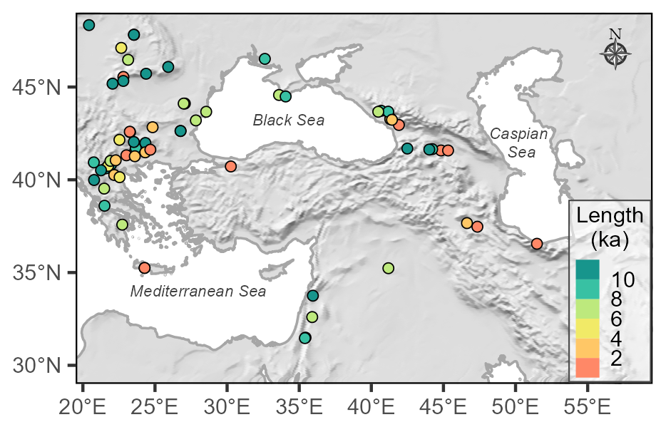
Figure 1 Distribution of pollen records used in the climate reconstructions. The colour coding shows the length of the record.

2.3 Climate reconstructions

We used tolerance-weighted, weighted-averaging partial least squares (fxTWA-PLS; Liu et al., 2020) regression to model the relationships between taxon abundances and individual climate variables in the modern training data set and then applied these relationships to reconstruct past climate using the fossil assemblages. fxTWA-PLS reduces the known tendency of regression methods to compress climate reconstructions towards the middle of the sampled range by applying a sampling frequency correction to reduce the influence of uneven sampling of climate space and by weighting the contribution of individual taxa according to their climate tolerance (Liu et al., 2020). Version 2 of fxTWA-PLS (fxTWA-PLS2; Liu et al., 2023), applied here, uses P-spline smoothing to derive the frequency correction and also applies the correction both in estimating climate optima and in the regression itself, producing a further improvement in model performance relative to version 1, as published by Liu et al. (2020).

We evaluated the fxTWA-PLS models by comparing the reconstructions against observations using pseudo-removed leave-out cross-validation, where one site was randomly selected as a test site and geographically and climatically similar sites (pseudo sites) were removed from the training set to avoid redundancy in the climate information inflating the cross-validation. We selected the last significant component (p value ≤ 0.01) and assessed model performance using the root mean square error of the prediction (RMSEP). The degree of compression was assessed using linear regression, and local compression was assessed by loess regression (locfit). Climate reconstructions were made for every sample in each fossil record using the best models, and sample-specific errors were estimated via bootstrapping. We applied a correction factor (Prentice et al., 2022a) to the reconstructions of α to account for the impact of changes in atmospheric CO₂ levels on water use efficiency, specifically the increased water use efficiency under high CO₂ levels characteristic of the recent past and the low CO₂ levels that would have reduced water use efficiency during the Late Glacial period and thus could have influenced the reconstructions during the earliest part of the records. The correction was implemented through the package codos: 0.0.2 (Prentice et al., 2022b), with past CO₂ concentration values derived from the EPICA Dome C record (Bereiter et al., 2015).

2.4 Construction of climate time series

To obtain climate time series representative of the regional trends in climate, we first screened the reconstructions to remove individual samples with (a) low effective diversity (< 2), as measured using Hill's N2 diversity measure (Hill, 1973), which could indicate low pollen counts or local contamination; and (b) sample-specific errors above the 0.95 quantile to remove obvious outliers. This screening resulted in the exclusion of only a small number of individual samples (see Fig. S2). We then averaged the reconstructed values in 300-year bins (slightly larger than the average resolution of the records at 228 years) with 50 % overlap. The first bin centred on 150 years before present, and subsequent bins were centred at 150-year increments throughout the record. We excluded any bins with only one sample. The binned values of individual sites were averaged to produce a regional composite of the anomalies for each climate variable, where the modern baseline was taken as the first 300-year bin centred on 150 years before present. These time series were smoothed using locally weighted regression (Cleveland and Devlin, 1988), with a window width of 1000 years (half-window width 500 years) and fixed target points in time to highlight the long-term trends. Confidence intervals (5th and 95th percentiles) for each composite were generated by bootstrap resampling by site over 1000 iterations. We examined the impact of the CO₂ correction on reconstructed α (Fig. S3); this had no major effect on the reconstructed trends, except during the earliest part of the record.

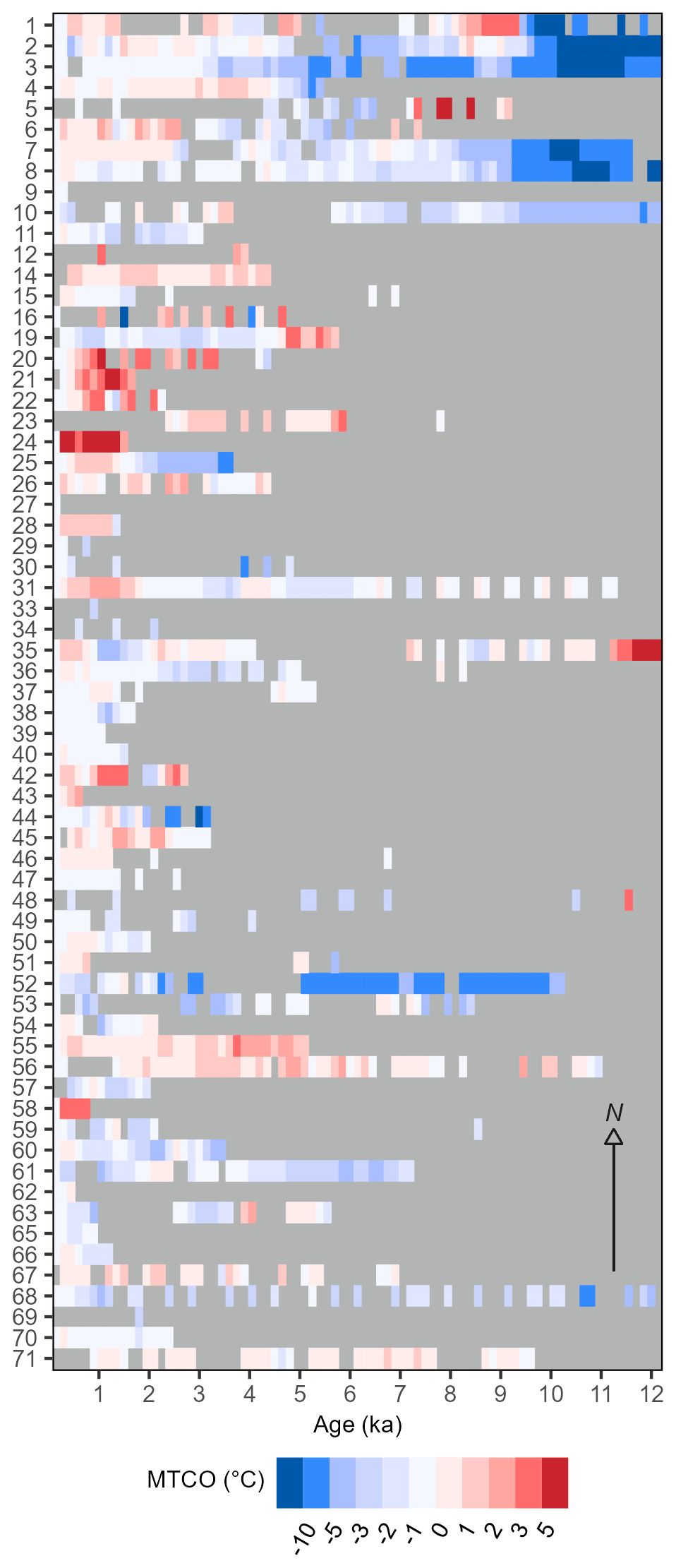
Figure 2 Time series of reconstructed anomalies of mean temperature of the coldest month (MTCO) for individual records. Entities are arranged by latitude (N–S). Information about the numbered individual sites can be found in Table S1.

2.5 Climate model simulations

We compared the reconstructed climate changes with transient climate model simulations of the response to external forcing to determine the extent that the reconstructed climate changes reflect changes in known forcing. We used transient simulations of the response to orbital and greenhouse gas forcing in the later Holocene from the following four models participating in the PAleao-Constraints on Monsoon Evolution and Dynamics (PACMEDY) project (Carré et al., 2021): the MPI (Max Planck Institute) Earth System Model version 1.2 (Dallmeyer et al., 2020), the AWI (Alfred Wegener Institute) Earth System Model version 2 (Sidorenko et al., 2019), and two versions of the IPSL (Institut Pierre-Simon Laplace) Earth System Model. The IPSL and AWI simulations were run from 6 ka to 1950 CE and the MPI simulation from 7.95 ka to 1850 CE. We used a longer transient simulation covering the period from 11.5 ka that was made with the LOVECLIM model (Goosse et al., 2010), which, in addition to orbital and greenhouse gas forcing, accounts for the waning of the Laurentide and Fennoscandian ice sheets (Zhang et al., 2016). Finally, we used two transient simulations from 22 ka to the present that were made using the Community Climate System Model (CCSM3; Collins et al., 2006). Both were forced by changes in orbital configuration, atmospheric greenhouse gas concentrations, continental ice sheets, and meltwater fluxes but differ in the configuration of the meltwater forcing applied after the Bølling warming (14.7 ka). In the first simulation (TRACE-21k-I; Liu et al., 2009), there was a sustained meltwater flux of ∼ 0.1 Sv from the Northern Hemisphere ice sheets to the Arctic and North Atlantic until ca. 6 ka and a continuous inflow of water from the North Pacific into the Arctic after the opening of the Bering Strait. The second simulation (TRACE-21k-II; He and Clark, 2022) had no meltwater flux during the Bølling warming or the Holocene but applied a flux of ∼ 0.17 Sv to the North Atlantic during the Younger Dryas (12.9–11.7 ka). The difference in meltwater forcing results in a much stronger Atlantic Meridional Overturning Circulation during the Holocene in the TRACE-21k-II simulation compared to the TRACE-21k-I simulation. Details of the model simulations are given in Table S3. The use of multiple simulations allows the identification of robust signals that are not model-dependent (see, e.g., Carré et al., 2021) and also the separation of the effects of different forcings. The TRACE-21k-I data were adjusted to reflect the changing length of months during the Holocene (related to the eccentricity of Earth's orbit and the precession-determined time of year of perihelion), whereas the other simulations were not. However, this makes little practical difference for the selection of variables used here (Fig. S4).

Outputs from each simulation were extracted for land grid cells in the EMBSeCBIO domain (29–49^∘ N, 20–55^∘ E; this region extends slightly less far eastwards than the EMBSeCBIO region as originally defined, but there are no pollen sites beyond 55^∘ E). The MTCO and MTWA were extracted directly; GDD0 was obtained by deriving daily temperature values from monthly data using a mean-preserving autoregressive interpolation function (Rymes and Myers, 2001). Daily values of cloud cover fraction and precipitation were obtained from monthly data in the same way and used to estimate MI, i.e. the ratio of annual precipitation to annual potential evapotranspiration, through the R package smpds (Villegas-Diaz and Harrison, 2022) before converting this to α, following Liu et al. (2020). For consistency with the reconstructed time series, climate anomalies for 30-year bins for each land grid cell within the EMBSeCBIO domain were calculated using the interval after 300 years before present as the modern baseline. Since the spatial resolution of the models varies (Table S3), and in any case is coarser than the sampling resolution of the individual pollen records precluding direct comparisons except at a regional scale, we used all of the land grid cells within the EMBSeCBIO domain and did not attempt to select grid cells coincident with the location of pollen data. A composite was produced by averaging the grid cell time series, which was then smoothed, using locally weighted regression (Cleveland and Devlin, 1988) with a window width of 1000 years (i.e. a half-window width of 500 years) and fixed target points in time. Confidence intervals (5th and 95th percentiles) for each composite were generated by bootstrap resampling by grid cell over 1000 iterations.

3 Results

3.1 Performance of the fxTWA-PLS statistical model

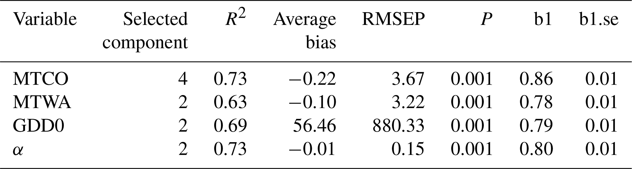
The assessment of the model through cross-validation showed that it reproduces the modern climate variables reasonably well (Table 1; Table S4). The best performance is achieved by α (R²= 0.73; RMSEP = 0.15) and MTCO (R²= 0.73; RMSEP 3.67). The models for GDD0 (R²= 0.69; RMSEP = 880) and MTWA (R²= 0.63, RMSEP = 3.22) were also acceptable. The slopes of the regressions ranged from 0.78 (MTWA) to 0.86 (MTCO), indicating that the degree of compression in the reconstructions in small (Table 1). Thus, the downcore fxTWA-PLS reconstructions of all the climate variables can be considered to be robust and reliable.

Table 1 Leave-out cross-validation fitness of fxTWA-PLSv2 for the mean temperature of the coldest month (MTCO), mean temperature of the warmest month (MTWA), growing degree days above base level 0 ^∘C (GDD0), and plant-available moisture (α), with a P-spline-smoothed fx estimation, using bins of 0.02, 0.02, and 0.002, showing results for the selected component for each variable. RMSEP is the root mean square error of the prediction. P assesses whether using the current number of components is significantly different from using one component less. The degree of overall compression is assessed by linear regression of the cross-validated reconstructions onto the climate variable, where b1 and b1.se are the slope and the standard error of the slope, respectively. The overall compression is reduced as the slope approaches 1. Full details for all the components are given in Table S4.

3.2 Holocene climate evolution in the region

Down-core reconstructions showed broadly coherent signals, although there was variation in both the timing and magnitude of climate changes across the sites that reflected differences in latitude and elevation (Figs. 2, 3, 4). Nevertheless, the records indicated coherent regional trends over the past 12 kyr.

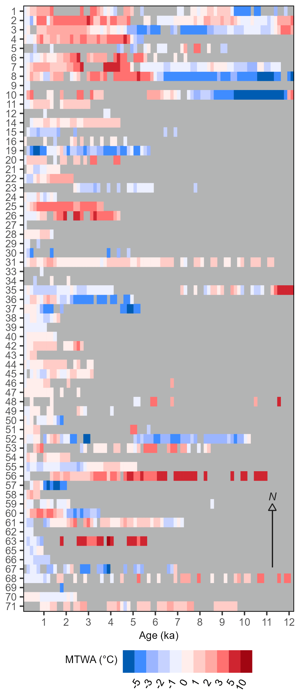
Figure 3 Time series of reconstructed anomalies of mean temperature of the warmest month (MTWA) for individual records. Entities are arranged by latitude (N–S). Information about the numbered individual sites can be found in Table S1.

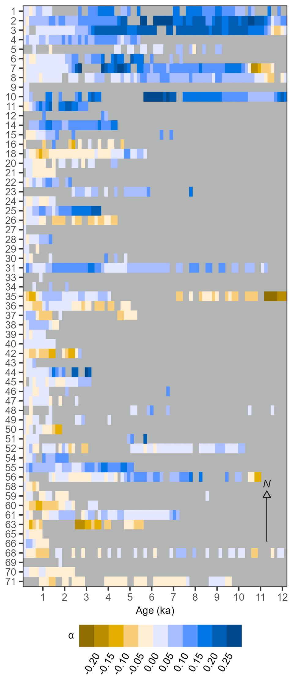
Figure 4 Time series of reconstructed anomalies of plant-available moisture, expressed as the ratio between potential and actual evapotranspiration (α), at individual sites. A correction to account for the direct physiological impacts of CO₂ on plant growth has been applied to the reconstructed α. Entities are arranged by latitude (N–S). Information about the numbered individual sites can be found in Table S1.

Winter temperature showed a cooling trend between 12 and 11 ka, with the reconstructed MTCO ca. 8 ^∘C lower than the present at 11 ka (Fig. 5). There was a moderate increase in the MTCO after 11 ka, followed by a more pronounced increase of ca. 5 ^∘C between 10.3 and 9.3 ka. Winter temperatures were only ca. 2 ^∘C lower than the present at the end of this rapid warming phase. There are relatively large uncertainties in the MTCO reconstructions prior to 10.3 ka, so the trends in the early part of the record are not well constrained. However, the phase of rapid warming between 10.3 and 9.3 ka (and the subsequent part of the record) is well constrained. MTCO continued to increase gradually through the Holocene, although multi-centennial to millennial oscillations were superimposed on the general trend.

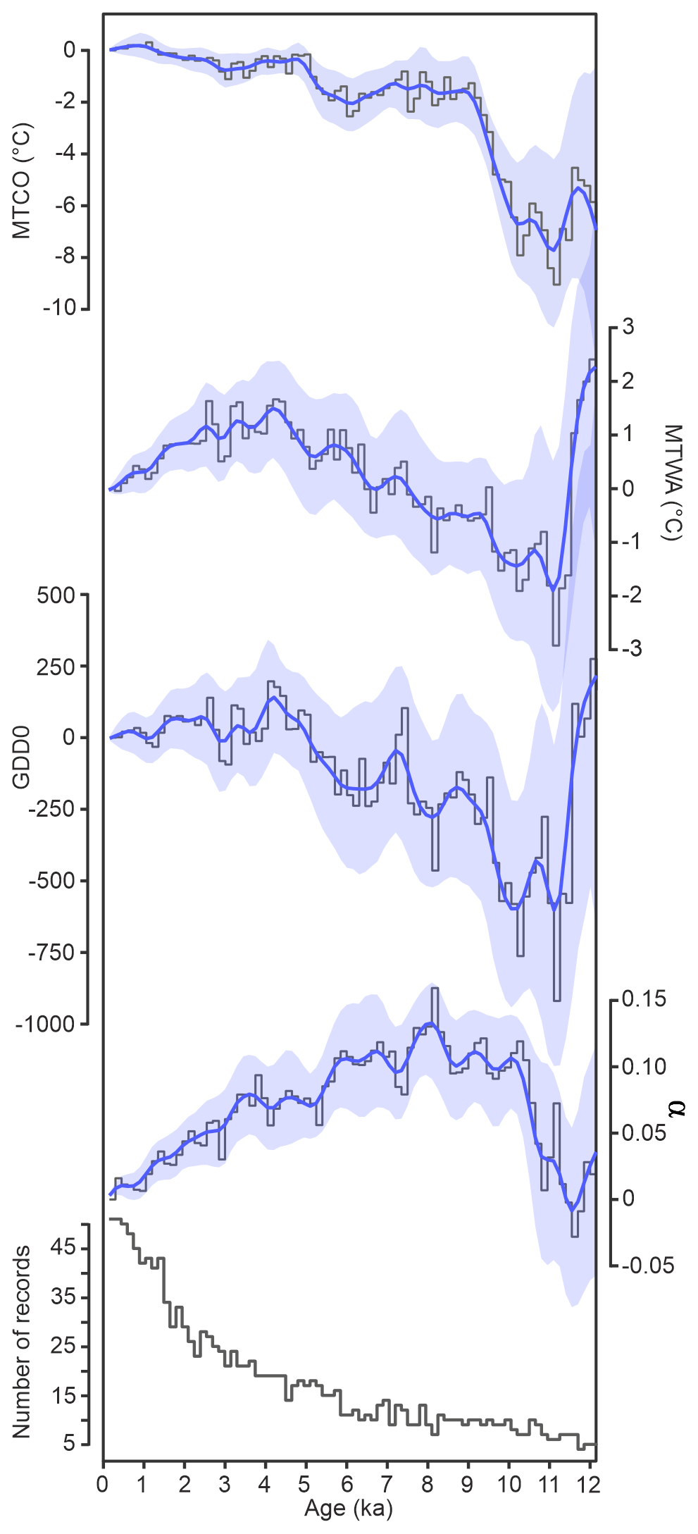
Figure 5 Composite changes in reconstructed mean temperature of the coldest month (MTCO), mean temperature of the warmest month (MTWA), growing degree days above a base level of 0 ^∘C (GDD0), and plant-available moisture expressed as the ratio between potential and actual evapotranspiration (α). A correction to account for the direct physiological impacts of CO₂ on plant growth has been applied to the reconstructions of α. The dark blue line is a loess smoothed curve through the reconstruction, with a window half-width of 500 years; the green shading shows the uncertainties based on 1000 bootstrap resampling of the records. The bottom plot shows the number of records used to create the composite through time.

The initial trends in the summer temperature were broadly similar to those in MTCO, with a cooling between 12.3 and 11 ka and the reconstructed MTWA ca. 2 ^∘C lower than the present at 11 ka (Fig. 5). Summer temperature increased thereafter, although with pronounced millennial oscillations, up to ca. 4.5 ka when the MTWA was ca. 1.5 ^∘C higher than the present. There was a gradual decrease in summer temperature after ca. 4.5 ka. The GDD0 reconstructions showed similar trends to the MTWA, reaching maximum values around 4.5 ka when the growing season was ca. 150 degree days greater than today. The subsequent decline in GDD0 was somewhat flatter, which presumably reflects the influence of still-increasing winter temperatures on the length of the growing season.

The trends in α differ from the trends in temperature. Conditions were similar to the present at around 11.5 ka (Fig. 5). Between 11 and 10 ka, there was a rapid increase in α. Values of α were higher than the present (> 0.1) between 10 to 6 ka. Subsequently, there was a gradual and continuous decrease in α until the present time. The correction for the physiological impact of CO₂ levels was, as expected, largest during intervals when CO₂ was lowest (i.e. prior to 11 ka; Fig. S4). The reconstructions with and without the correction are not statistically different between 10 and 5 ka, when taking account the uncertainties in the reconstructions, but the correction produced marginally wetter reconstructions after 5 ka, with a maximum difference of 0.08. However, the gradually declining trend in moisture availability towards the present is not affected by the CO₂ correction.

3.3 Comparison with climate simulations

The TRACE-21k-I simulation (Fig. 6) shows an initial winter warming between 12 and 11 ka, but the MTCO is still ca. 3 ^∘C lower than the present at 11 ka. There is a gradual increase in MTCO from 11 ka onwards, although with centennial-scale variability and a more pronounced oscillation corresponding to the 8.2 ka event. The TRACE-21k-II simulation is initially slightly colder and displays a two-step warming, with a peak at 8.5 ka, when MTCO is ca. 1.5 ^∘C lower than the present. The later Holocene trend is similar to that shown in TRACE-21k-I. The LOVECLIM simulation produced generally warmer conditions than either of the TRACE simulations, where MTCO is ca. 2.5 ^∘C lower than the present at 11 ka, but the two-step warming is more pronounced, and peak warming occurs somewhat later, at ca. 7.5 ka, when the MTCO was only ca. 0.25 ^∘C lower than the present (Fig. 7). While all three models show a rapid warming comparable to the reconstructed warming between 10.3 and 9.3 ka, it is clear that the differences in the ice sheet and meltwater forcings affect both the magnitude and the timing of this trend. The overall magnitude of the warming after 9 ka in the TRACE-21k-I simulation is consistent with the reconstructions of the MTCO (anomalies of 2.4 and 2.6 ^∘C for model and data, respectively). The mid to late Holocene trend is similar in the PACMEDY simulations (Fig. 8) to both TRACE-21k simulations, both in sign and in magnitude (ca. 1 ^∘C between 6 ka and the present), and both are consistent with the reconstructions ($-\mathrm{0.9}\pm \mathrm{0.7}$ ^∘C). The continuous increase in MTCO is consistent with the change in winter insolation. Given the similarities between the PACMEDY simulations (which only include orbital and greenhouse gas forcing) and the LOVECLIM and TRACE simulations, which also include the forcing associated with the relict Laurentide and Fennoscandian ice sheets, it seems likely that orbital forcing was the main driver of winter temperatures in the EMBSeCBIO region during the later Holocene.

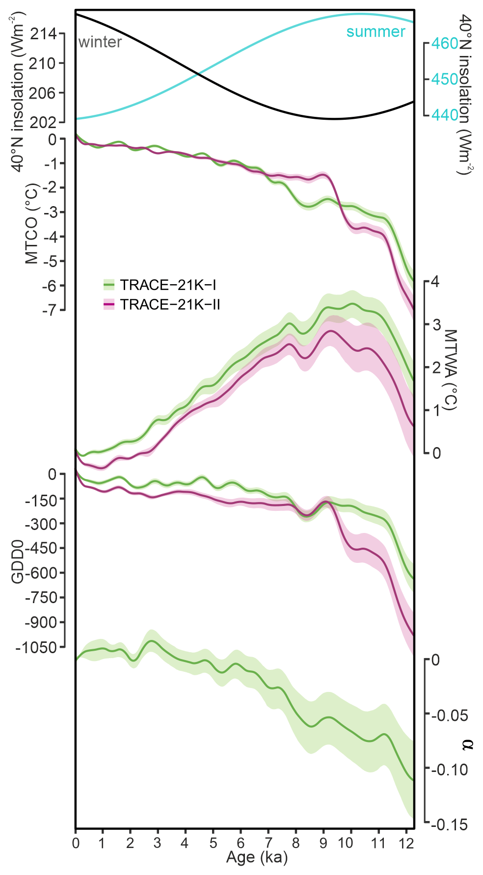
Figure 6 Simulated regional changes in mean temperature of the coldest month (MTCO), mean temperature of the warmest month (MTWA), growing degree days above a base level of 0 ^∘C (GDD0), and plant-available moisture expressed as the ratio between potential and actual evapotranspiration (α) in the EMBSeCBIO domain from the TRACE-21K-I (green) and TRACE-21K-II (red) transient simulations. It is not possible to calculate changes in α for the TRACE-21K-II simulation from the available data. Loess smoothed curves were drawn using a window half-width of 500 years, and the envelope was obtained through 1000 bootstrap resampling of the sequences. The top plot shows the changes in summer and winter insolation (Wm⁻²) at 40^∘ N.

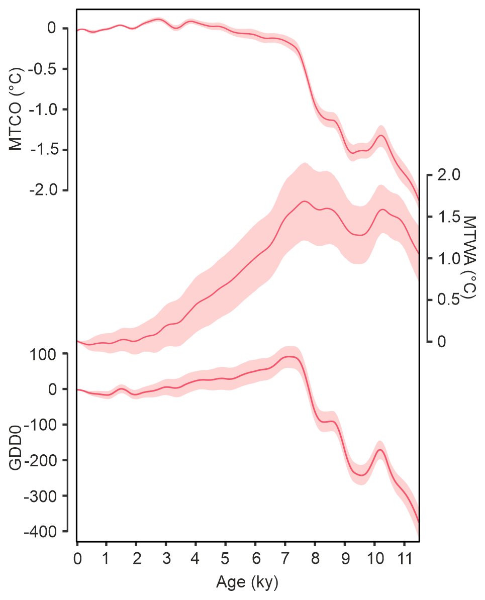
Figure 7 Simulated regional changes in mean temperature of the coldest month (MTCO), mean temperature of the warmest month (MTWA), and growing degree days above a base level of 0 ^∘C (GDD0) in the EMBSeCBIO domain from the LOVECLIM transient simulation. It is not possible to calculate the changes in α for the LOVECLIM simulation from the available data. Loess smoothed curves were drawn using a window half-width of 500 years, and the envelope was obtained through 1000 bootstrap resampling of the sequences.

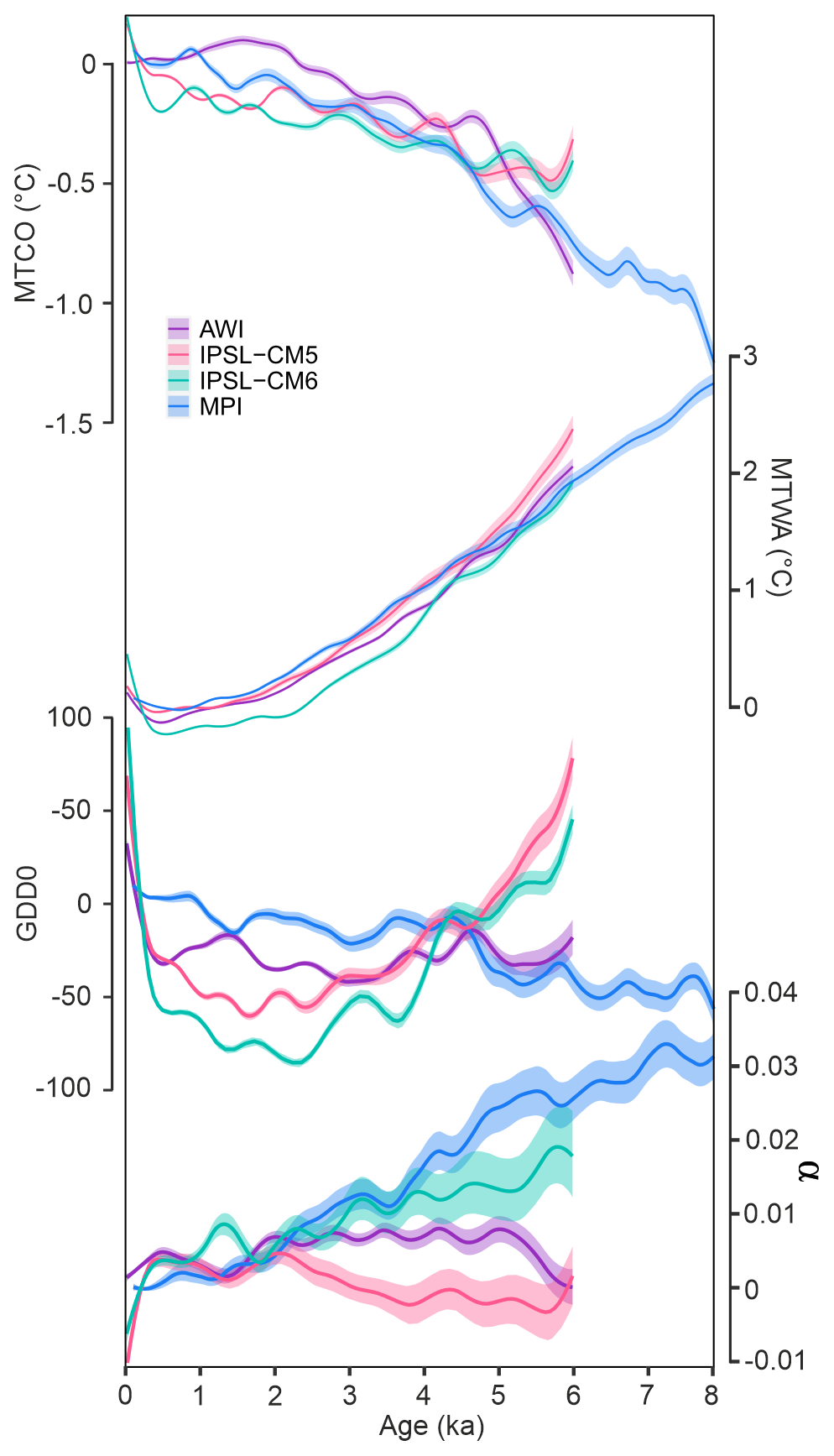
Figure 8 Simulated regional changes in the mean temperature of the coldest month (MTCO), mean temperature of the warmest month (MTWA), and growing degree days above a base level of 0 ^∘C (GDD0) in the EMBSeCBIO domain from the four PACMEDY simulations. The models are the Max Plank Institute Earth System Model (MPI), Alfred Wegener Institute Earth System Model simulations (AWI), Institut Pierre-Simon Laplace Climate Model TR5AS simulation (IPSL-CM5), and Institut Pierre-Simon Laplace Climate Model TR6A V simulation (IPSL-CM6). Loess smoothed curves were drawn using a window half-width of 500 years and the envelope was obtained through 1000 bootstrap resampling of the sequences.

The TRACE-21k-I simulation shows peak summer temperatures between 11 and 9 ka, when the MTWA was ca. 3 ^∘C greater than the present (Fig. 6). The TRACE-21K-II simulations are initially colder than the TRACE-21k-I simulation, and the peak in summer temperatures occurs at 9 ka, when the MTWA was ca. 2.5 ^∘C greater than the present (Fig. 6). The LOVECLIM simulation is warmer than the present from 11.5 ka, but peak warming is only reached at 7.5 ka when the MTWA is ca. 2 ^∘C (Fig. 7). All three simulations show a gradual decrease in the summer temperature through the Holocene after this initial peak. This decreasing trend is also seen in the PACMEDY simulations from 6 ka (or 8 ka in the case of the MPI simulation) onwards (Fig. 8), and the magnitude of the change over this interval (ca. 2 ^∘C from 6 ka onwards) is similar to that shown by the TRACE and the LOVECLIM simulations. This similarity suggests that the simulated response is a direct reflection of the change in orbital forcing. However, the reconstructed changes in summer temperature do not show this gradual decline. Reconstructed MTWA is ca. 4 ^∘C colder than the model predictions at 9 ka. The reconstructions show a gradual increase in the MTWA from 9 to 4.5 ka. Changes in reconstructed temperatures at 4.5 ka are of a similar magnitude to the simulated temperatures at this time (ca. 1 ^∘C greater than the present), although the late Holocene is marked by a cooling trend, as seen in the simulations. Thus, while the simulated late Holocene trend is consistent with orbital forcing being the main driver of summer temperatures in the EMBSeCBIO region, the early to mid Holocene trend is not. Previous modelling studies have suggested that the timing of peak warmth differs in different regions of Europe and is associated with the impact of the Fennoscandian ice sheet on regional climates (Renssen et al., 2009; Blascheck and Renssen, 2013; Zhang et al., 2016). The differences in the timing of peak warmth in the EMBSeCBIO region in the TRACE-21k-II and LOVECLIM simulations would be consistent with this argument but suggest that the timing and magnitude are model-dependent. It is therefore plausible that the reconstructed trend in the MTWA at least during the early Holocene reflects the influence of the relict Laurentide and Fennoscandian ice sheets in modulating the impact of increased summer insolation until the mid Holocene. Given that GDD0 is a reflection of both changes in season length, as influenced by winter temperatures and summer warming, the difference between the simulated and reconstructed MTWA are also seen in GDD0 trends during the early part of the Holocene (Fig. 6).

The simulations do not show consistent patterns for the trend in α. The TRACE-21k-I simulation (Fig. 6) shows a gradual increase, with minor multi-centennial oscillations from 12 ka to present. (Available model output variables are not sufficient to calculate α for the TRACE-21k-II or LOVECLIM simulations.) One of the PACMEDY simulations (IPSL-CM5) shows an increase from the mid Holocene (Fig. 8), although the simulated change is an order of magnitude smaller than over the comparable period in the TRACE-21k-I simulation. The AWI model shows no trend in α over this period; the remaining two models show increasing aridity from the mid Holocene to the present (Fig. 8). These three models are all broadly consistent with the reconstructions, since the reconstructed decrease in α is small. However, the differences in the sign of the trend between the different models indicates that changes in moisture are not a straightforward consequence of the forcing but must reflect model-dependent changes in moisture supply via changes in atmospheric circulation. Reconstructions of Holocene climates in Iberia have suggested that land–surface feedbacks associated with changes in moisture availability have a strong influence on summer temperature (Liu et al., 2023). There does not seem to be strong evidence for this in the EMBSeCBIO region, given the difference in the trends of α and the MTWA and the muted nature of the trend in α.

4 Discussion

The three temperature-related variables, MTCO, MTWA, and GDD0, all show relatively warm conditions around the late glacial–Holocene transition (ca. 12 ka), followed by a cooling that was greatest between ca. 11 and 10 ka. This pattern is also shown in regional composites (Fig. 9) derived from the reconstructions by Mauri et al. (2015) and Herzschuh et al. (2022). However, the magnitude of the cooling shown in the Mauri et al. (2015) and Herzschuh et al. (2022) reconstructions is small compared to our reconstructions. The cool interval starts somewhat later and persists until 9 ka in the Mauri et al. (2015) reconstructions, but this is partly a reflection of the fact that these reconstructions were only made at 1 ka intervals, and thus, the transitions are less well constrained than in either our reconstructions or those of Herzschuh et al. (2022). This cool interval and the marked warming seen after 10.3 ka in our reconstructions does not correspond to the Younger Dryas and the subsequent warming. Although the Younger Dryas is considered to be a globally synchronous event (Cheng et al., 2020) and is generally considered coeval with Greenland stadial I (Larsson et al., 2022), it does not appear to be strongly registered in the EMBSeCBIO region in any of the quantitative climate reconstructions. This is consistent with earlier suggestions, based on vegetation changes, that the Younger Dryas was not a clearly marked feature over much of this region (Bottema, 1995).

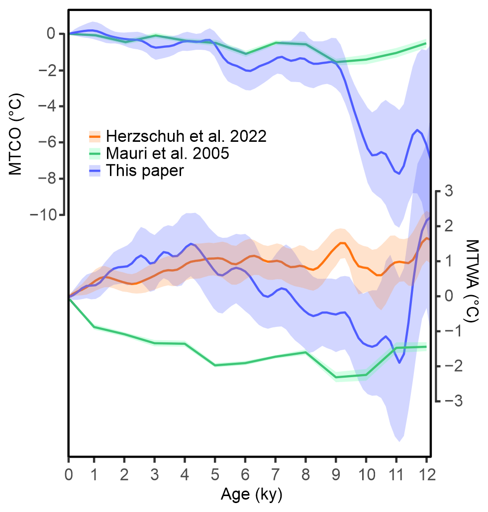
Figure 9 Comparison of regional composites of reconstructed seasonal temperatures from this study with those derived from Mauri et al. (2015) and Herzschuh et al. (2022). Mauri et al. (2015 provide the mean temperature of the coldest month (MTCO) and mean temperature of the warmest month (MTWA) reconstructions, which can be directly compared with our reconstructions. Herzschuh et al. (2022) only provide reconstructions of July temperature. Our reconstructions are shown in blue, reconstructions based on the Mauri et al. (2015) data set are shown in green, and reconstructions based on the Herzschuh et al. (2022) reconstruction are shown in orange. The solid line is a loess smoothed curve through the reconstruction with a window half-width of 500 years; the shading shows the uncertainties based on 1000 bootstrap resampling of the records.

We have shown that winter temperatures increased sharply between 10.3 and 9.3 ka but then continued to increase at a more gradual rate through the Holocene. The increase of ca. 7.5 ^∘C is of the same order of magnitude to the increase shown in the TRACE-21K-II simulation (ca. 5 ^∘C) and in the LOVECLIM simulation (ca. 3 ^∘C). This increasing trend is also seen in the Mauri et al. (2015) reconstructions of MTCO (Fig. 9), although the change from the early Holocene to the present is much smaller (ca. 0.5–1 ^∘C) in these reconstructions than in our reconstructions, and Mauri et al. (2015) do not show marked cooling around 11 ka. Nevertheless, the consistency between the two reconstructions and between our reconstruction and the simulated changes in MTCO supports the idea that these trends are a response to orbital forcing during the Holocene. Our reconstructions show a gradual increase in summer temperature, as measured by both MTWA and GDD0, from ca. 10 to 5 ka, when the MTWA was ca. 1 ^∘C warmer than the present, followed by a gradual decrease towards the present. This is not consistent with previous reconstructions. Mauri et al. (2015) show an overall increasing trend from 9 ka to present. The Herzschuh et al. (2022) study shows a completely different pattern, with the maximum in July temperature at ca. 9 ka and an oscillating but declining trend thereafter (Fig. 9).

These differences between the three sets of reconstructions are too large to be caused by differences in the age models applied. They are also unlikely to reflect differences in sampling, since the number of sites used is roughly similar across all three reconstructions (71 sites versus 67 sites from Herzschuh et al., 2022, and 409 grid points, based on 57 sites, from Mauri et al., 2015); most sites are common to all three analyses. The differences must therefore be related to the reconstruction method. Herzshuch et al. (2022) used the regression-based approach, weighted-average partial least squares (WA-PLS) that is the basis for our reconstruction technique, fxTWA-PLSv2. Mauri et al. (2015) used the modern analogue technique. However, after taking the differences caused by the temporal resolution into account, there is greater similarity between our reconstructions and those of Mauri et al. (2015) than between either of these reconstructions and the Herzschuh et al. (2022) reconstructions.

Several methodological issues could be responsible for the differences between the three sets of reconstructions and, in particular, the anomalous moisture trends shown by Herzschuh et al. (2022). Specifically, Herzschuh et al. (2022) used (1) a unique calibration data set for each fossil site, based on modern samples within a 2000 km radius of that site, rather than relying on a single training data set; (2) a limited set of 70 dominant taxa rather than the whole pollen assemblage; and (3) marine records, including those from, e.g., the Black Sea, which were excluded in the other reconstructions because they sample an extremely large area and thus are unrepresentative of the local climate. However, inclusion of records from the Black Sea in our reconstructions does not have a substantial impact on either the magnitude or the trends in climate. Thus, it seems likely that the differences between these two reconstructions reflects the use of a unique calibration data set for each fossil site and the limited set of taxa included.

The reconstructed MTWA shows a gradual increase through the early Holocene with maximum values of around 1.5 ^∘C greater than the present reached at ca. 4.5 ka. Previous modelling studies have shown that the timing of maximum warmth during the Holocene in Europe was delayed compared to the maximum of insolation forcing and varied regionally as a consequence of the impact of the Fennoscandian ice sheet on surface albedo, atmospheric circulation, and heat transport (Renssen et al., 2009; Blascheck and Renssen, 2013; Zhang et al., 2016; Zhang et al., 2018). Two of the simulations examined here show a delay in the timing of peak warmth, which occurred ca. 9 ka in the TRACE-21k-II simulation and ca. 7.5 ka in the LOVECLIM simulation. Although both sets of simulations include the relict Laurentide and Fennoscandian ice sheets, neither has realistic ice sheet and meltwater forcing. In the LOVECLIM simulation, for example, the Fennoscandian ice sheet was gone by 10 ka, whereas in reality it persisted until at least 8.7 ka (Patton et al., 2017). Thus, the impact of the Fennoscandian ice sheet in delaying orbitally induced warming would likely have been greater than shown in this simulation. In addition to differences in the way in which ice sheets and meltwater forcing are implemented in different models, models are also differentially sensitive to the presence of the same prescribed ice sheet (Kapsch et al., 2022). Thus, it would be useful to examine the influence of more realistic prescriptions of the relict ice sheets on the climate of the EMBSeCBIO region using multiple models and, preferably, transient simulations at a higher resolution or with regional climate models. It has been suggested that meltwater was routed to the Black and Caspian seas via the Dnieper and Volga rivers during the early phase of deglaciation (e.g. Yanchilina et al., 2019; Aksu et al., 2022; Vadsaria et al., 2022), and it would also be useful to investigate the impact of this on the regional climate.

We have shown that α was similar to today around 11 ka, but there was a rapid increase in moisture availability after ca. 10.5 ka, such that α values were noticeably higher than the present between 10 to 6 ka, followed by a gradual and continuous decrease until the present time. Changes in the late Holocene are small even at centennial scale (Fig. 5). The reconstructed trends in α are not captured in the simulations, which show different trends during the late Holocene. Thus, it is unlikely that the gradual increase in aridity during the late Holocene is a straightforward response to orbital forcing. Changes in α in the EMBSeCBIO region are likely to be primarily driven by precipitation changes, which in turn are driven by changes in atmospheric circulation. Differences in the trend of moisture availability between the models imply that the nature of the changes in circulation varies between models and thus the simulations do not provide a strong basis for explaining the observed patterns of change in moisture availability. Earlier studies, focusing on the western Mediterranean (Liu et al., 2023), Europe (Mauri et al., 2014), and central Eurasia (Bartlein et al., 2017), have shown that models have difficulty in simulating the enhanced moisture transport into the Eurasian continent shown by palaeoenvironmental data during the mid Holocene and during the late Holocene. Changes in precipitation can also affect land–surface feedbacks. Liu et al. (2023), for example, have argued that enhanced moisture transport into the Iberian peninsula during the mid Holocene led to more vegetation cover and increased evapotranspiration and had a significant impact on the reduction of growing season temperatures. Differences in the reconstructed trends of summer temperature and plant-available moisture through the Holocene suggests that this land–surface feedback was not an important factor influencing summer temperatures in the EMBSeCBIO region. Nevertheless, differences in the strength of land–surface feedbacks between models could also contribute to the divergences seen in the simulations. It would be useful to investigate the role of changes in atmospheric circulation for precipitation patterns during the Holocene in the EMBSeCBIO region using transient simulations at a higher resolution or with regional climate models.

The timing of the transition to an agriculture economy in the eastern Mediterranean is still debated (Asouti and Fuller, 2012). It has been argued that climatic deterioration and population growth during the Younger Dryas triggered a shift to farming (Weiss and Bradley, 2001; Bar-Yosef, 2017). The presence of morphologically altered cereals by the end of the Pleistocene has been put forward as evidence for an early transition to agriculture (Bar-Yosef et al., 2017), but it has also been pointed out that the evidence for cereal domestication before ca. 10.5 ka is poorly dated and insufficiently documented (Nesbitt, 2002) and that crops did not replace foraging economies until well into the Holocene (Smith, 2001; Willcox, 2012; Zeder, 2011). The availability of water is a crucial factor in the viability of early agriculture (Richerson et al., 2001; Zeder, 2011). We have shown that moisture availability was higher than today during the first part of the Holocene (10–6 ka) but similar to today until ca. 10.5 ka. Wetter conditions during the early Holocene could have been a crucial factor in the transition to agriculture, and our findings support the idea that this transition did not happen until much later than the Younger Dryas or late glacial–Holocene transition. Further exploration of the role of climate in the transition to agriculture would require a more comprehensive assessment of the archaeobotanical evidence. The issue could also be addressed by using modelling to explore how the reconstructed changes in regional moisture availability and seasonal temperatures would impact crop viability (see, e.g., Contreras et al., 2019).

We have focused on the composite picture of regional changes across the EMBSeCBIO region, in order to investigate whether these changes could be explained as a consequence of known changes in forcing. The data set also provides information on the trends in climate at individual sites. These data could be used to address the question of whether population density or cultural changes reflect shifts in climate (e.g. Weninger et al., 2006; Drake, 2012; Kaniewski et al., 2013; Cookson et al., 2019; Weiberg et al., 2019; Palmisano et al., 2021). In addition, it would also be possible to use these data to explore the impact of climate changes on the environment, including the natural resources available for people (Harrison et al., 2023).

5 Conclusions

We have reconstructed changes in seasonal temperature and in plant-available moisture from 12.3 ka to the present from 71 sites from the EMBSeCBIO domain to examine changes in the regional climate of the eastern Mediterranean region. We show that there are regionally coherent trends in these variables. The large increase in both summer and winter temperatures during the early Holocene considerably post-dates the warming observed elsewhere at the end of the Younger Dryas, supporting the idea that the impact of the Younger Dryas in the EMBSeCBIO region was muted. Subsequent changes in winter temperature are consistent with the expected response to insolation changes. The timing of peak summer warming occurred later than expected as a consequence of insolation changes and likely, at least in part, reflects the influence of the relict Laurentide and Fennoscandian ice sheets on the regional climate. There is a rapid increase in plant-available moisture between 11 and 10 ka, which could have promoted the adoption of agriculture in the region.