the Creative Commons Attribution 4.0 License.
the Creative Commons Attribution 4.0 License.
 | 13 Sep 2023
Do phenomenological dynamical paleoclimate models have physical similarity with Nature? Seemingly, not all of them do
Mikhail Y. Verbitsky
Michel Crucifix
Phenomenological models may be impressive in reproducing empirical time series, but this is not sufficient to claim physical similarity with Nature until comparison of similarity parameters is performed. We illustrated such a process of diagnostics of physical similarity by comparing the phenomenological dynamical paleoclimate model of Ganopolski (2023), the van der Pol model (as used by Crucifix, 2013), and the model of Leloup and Paillard (2022) with the physically explicit Verbitsky et al. (2018) model that played a role of a reference dynamical system. We concluded that phenomenological models of Ganopolski (2023) and of Leloup and Paillard (2022) may be considered to be physically similar to the proxy parent dynamical system in some range of parameters, or in other words they may be derived from basic laws of physics under some reasonable physical assumptions. We have not been able to arrive at the same conclusion regarding the van der Pol model. Though developments of better proxies for the parent dynamical system should be encouraged, we nevertheless believe that the diagnostics of physical similarity, as we describe it here, should become a standard procedure to delineate a model that is merely a statistical description of the data from a model that can be claimed to have a link with known physical assumptions.
The similarity parameters we advance here as the key dimensionless quantities are the ratio of the astronomical forcing amplitude to the terrestrial ice sheet mass influx and the so-called V number that is the ratio of the amplitudes of time-dependent positive and negative feedbacks. We propose using available physical models to discover additional similarity parameters that may play central roles in ice age rhythmicity. Finding values for these similarity parameters should become a central objective of future research into glacial–interglacial dynamics.
- Article
(2550 KB) - Full-text XML
- BibTeX
- EndNote


A mathematical model that is constructed to understand a physical phenomenon must be simple enough, otherwise the interpretation of the modeling results may be as difficult as the interpretation of direct observations. In that regard, even most sophisticated space-resolving models of global climate indeed provide a simplified picture of the phenomenon, but a much more drastic degree of simplification is required when we study climate on timescales of tens of thousands of years. Faced with this challenge, Barry Saltzman used to be a proponent of the phenomenological approach “through the construction of low-order models in which the full behavior is projected onto the dynamics of a reduced number of … highly aggregated variables” (Saltzman, 2002). Phenomenological models of paleoclimate variability have routinely been used to explain certain characteristics of glacial–interglacial cycles (e.g., Saltzman and Maasch, 1991; Saltzman and Verbitsky, 1992, 1993, 1994; Paillard, 1998; Tziperman et al., 2006; Crucifix, 2013; Kaufmann and Pretis, 2021; Talento and Ganopolski, 2021; Leloup and Paillard, 2022; Ganopolski, 2023). The core principle of the phenomenological approach is to fit model-produced time series to the observational time series. When this goal is achieved, it is tacitly assumed that there must be some physical similarity between the phenomenological model and Nature. However, we believe that the assumption of physical similarity with Nature can be more rigorously challenged before the implications of a phenomenological model are accepted.
In fluid dynamics, for example, the concept of physical similarity is the cornerstone of any judgment built on model experimentations. Classical similarity parameters, which emerge from the analysis of fundamental conservation laws, like the Reynolds number, the Péclet number, or the Euler number quantify the relative importance of different aspects of fluid flow. For an experimental or a numerical model to be relevant, it should have quantitatively the same similarity parameters as those of the natural phenomenon being considered. We will now apply this concept of physical similarity to dynamical paleoclimate systems.
As physicists, we might want to describe a phenomenon such as ice ages as “emerging from fundamental laws”. However, the fundamental laws that we know in physics dictate interactions between particles. Perhaps one of the greatest challenges of the physical approach to complex systems is to explain how Nature organizes billions of billions of particles in interaction to generate some predictable behavior even on very long timescales, such as glacial–interglacial cycles. The methods of statistical physics tell us how to define macroscopic variables to describe the collective behavior of particles submitted to a conservation constraint and how the phenomenon of dissipation emerges as a consequence of statistical mixing in a chaotic system. Dynamical systems theory tells us why we mainly see the most unstable modes of a system (Haken, 2006) and how timescale separation assumptions allow us to focus on a subset of the system's variables. In a nutshell, the theories of mathematical and statistical physics make it legitimate to assume that there is a natural parent dynamical system with far fewer degrees of freedom than Avogadro's number and which has generated the phenomenon that we see.
What “far fewer” means is not a straightforward matter. It depends on what we describe as the phenomenon and how fine-grained this description is. For example, the successions of glacial–interglacial cycles and the timing of deglaciations appear to follow fairly simple, predictable rules (Tzedakis et al., 2017). Hence, it is legitimate to assume that the physical parent dynamical system, which dictates the evolution of the macroscopic state of climate at the orbital timescale, can be reduced to a small number of degrees of freedom.
Specifically, we may suggest that this parent dynamical system is governed by n physical parameters ai such that a dependent variable of interest, x, can be expressed as the following function:
If k parameters of a1, a2, …, ai, …, an are parameters with independent dimensions, then according to π theorem (Buckingham, 1914), in the dimensionless form the phenomenon (Eq. 1) can be described by dimensionless similarity parameters Π1, Π2, …, Πi, …, Πm:
Two physical phenomena have physical similarity if both of them are described in the dimensionless form by the same function Φ(Π1, Π2, …, Πi, …, Πm) and have identical numerical values of similarity parameters Π1, Π2, …, Πi, …, Πm; however, numerical values of the governing parameters a1, a2, …, ai, …, an may be different (e.g., Barenblatt, 2003).
As we have already mentioned, our knowledge about a parent dynamical system is suggested to us by the presence of empirical time series. It means that one of the similarity parameters, say Π1, is dimensionless time (t and τ are dimensional time and a timescale, correspondingly), while all other parameters Π2, …, Πi, …, Πm are fixed to specific values. Hence, an experimental time series (neglecting measure errors) can be described as
If we created a model dynamical system such that it is governed by p governing parameters bi
and r parameters of b1, b2, …, bi, …, bp are parameters with independent dimensions, then again, according to π theorem, in the dimensionless form, the model can be described by dimensionless similarity parameters π1, π2, …, πi, …, πq:
For a specific time series and for a fixed set of parameters π2 …, πi, …, πq, the model (Eq. 5) can be presented as
The essence of the phenomenological approach is to fit the function to the function under the “best” set of parameters π2, …, πi, …, πq, i.e., to equate the model time series and the natural, empirical time series :
It is obvious that even if the goal (Eq. 7) is achieved at every point, we still cannot claim the model (Eq. 6) to be physically similar to Nature (Eq. 3) until we prove that πi=Πi, i.e., that πi physics in the model is as significant as the Πi physics of Nature. Simply speaking, merely matching a proposed phenomenological model with empirical data does not make a case for physical similarity because it does not provide evidence that it happens for the right reason, the reason being the similarity parameters of the right value, i.e., πi=Πi.
However, how can we compare πi physics of the phenomenological model and Πi physics of Nature if the phenomenological models are not derived from the laws of physics? Although phenomenological models indeed have not been derived from the laws of physics, they are not completely ignorant of the physical content: they still have a measurable physical variable, i.e., time, and they also have orbital and terrestrial forcings and positive and negative feedbacks. If the parent dynamical system was formulated in terms of similarity parameters formed by the ratios of timescales and by the ratios of the forcing and feedback amplitudes, then the comparison with phenomenological models that also use timescales and forcing and feedback ratios would be possible. The VCV18 model (Verbitsky et al., 2018) is one such candidate (a proxy) for a parent dynamical system. VCV18 was derived from the scaled mass and heat balance equations of the non-Newtonian ice flow. Next, we will derive scaling laws and similarity parameters for three phenomenological models: (a) the model of Ganopolski (2023), (b) the van der Pol model as it has been described by Crucifix (2013), and (c) the model of Leloup and Paillard (2022) (hereafter, G23, VDP, and LP22, respectively). Each of these models produces a specific function Ψ(π1, π2, …, πi, …, πq). We then compare the functions of Ψ(π1, π2, …, πi, …, πq) of these models with the corresponding function of Φ(Π1, Π2, …, Πi, …, Πm) provided by VCV18 to recognize or reject the hypothesis of physical similarity with a proxy for the parent dynamical system.
Certainly, we cannot expect that the time series produced by G23, VDP, and LP22 models and by the VCV18 model will be identical, and therefore these models will not be physically similar in the most rigorous sense of Eq. (7). We will demonstrate, however, that the answer to the physical-similarity question is insightful if our dependent variable of interest x is not necessarily a time series but a time-independent attribute such as the period of glacial rhythmicity. All models of this study reproduce the ∼100 kyr period of the Late Pleistocene glaciations equally well. We will now evaluate if the similarity parameters involved in the corresponding Eq. (7) are quantitatively the same.
2.1 VCV18 model as a proxy for a parent dynamical system
Deriving a low-order dynamical paleoclimate model that may be considered a candidate (a proxy) parent dynamical system is not a trivial exercise. The “low-order” challenge means that out of the multitude of physical phenomena involved only a few should be recognized as dominant, and the “dynamical” challenge means that the space-resolving properties should be sensibly reduced to some integrated variables. Accordingly, in developing VCV18 proxy parent dynamical system, we first assumed that ice ages can be explained by only two components of the global climate system, with continental ice sheets and the ocean representing the rest of the climate. For an ice sheet we adopted mass, momentum, and heat conservation equations of a “thin” layer of homogeneous non-Newtonian ice, and the rest of the climate was represented by the energy balance equation. To migrate from the three-dimensional to dynamical equations we used scaling analysis that provides simple mathematical statements that are consistent with the original physics. Accordingly, the VCV18 dynamical model of the ice–climate system is defined by the following set of equations:
Here, S (m2) is the area of glaciation, θ (∘C) is the basal ice sheet temperature, and ω (∘C) is the global temperature of the rest of the climate. Equation (8) represents global ice balance , where the ice thickness H is determined from the thin-layer approximation of ice flow, , ζ is dimensional profile factor (Verbitsky and Chalikov, 1986), and is the surface mass influx. Equation (9) describes vertical ice temperature advection with a timescale , and Eq. (10) is the global energy balance equation. The parameter (m s−1) is the snow precipitation rate; F is normalized external forcing, i.e., mid-July insolation at 65∘ N (Berger and Loutre, 1991) of the amplitude ε (m s−1); κω represents fast positive feedback from the global climate on ice sheet mass balance; and cθ is the ice discharge due to ice sheet basal sliding incorporating (both delayed due to the vertical temperature advection) positive feedback from the global temperature, αω, and a negative feedback of basal temperature reaction to the changes in ice geometry β[S−S0]. Further, is external forcing for global temperature (e.g., albedo); κ (m s−1 ∘C−1), c (m s−1 ∘C−1), α (dimensionless), β (∘C m−2), and γ (∘C m−2 s−1) are sensitivity coefficients; S0 (m2) is a reference glaciation area; and τ (s) is the global-temperature timescale.
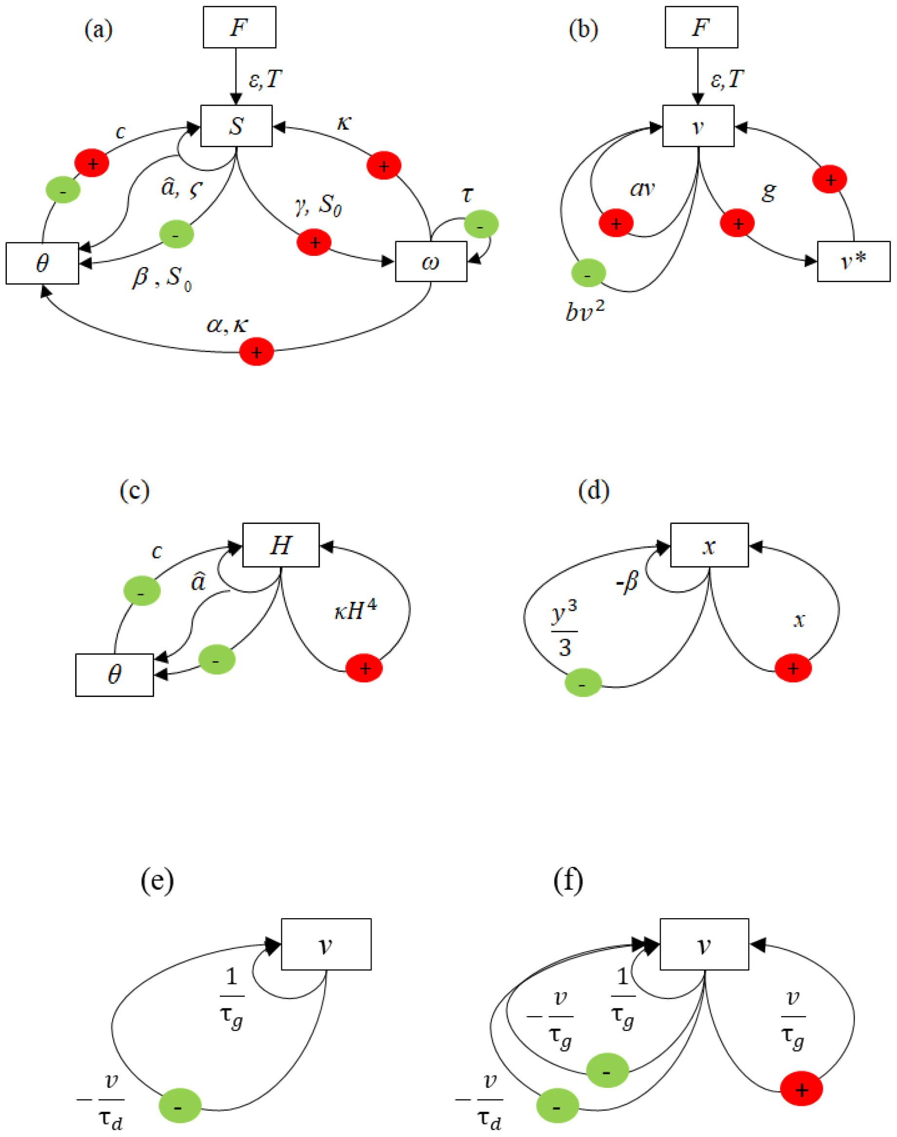
Figure 1(a) The parent dynamical system VCV18 (Eqs. 8–10). Red circles mark positive feedback loops, and green circles mark negative feedback loops. (b) The same as (a) but for the G23 phenomenological model (Eqs. 12 and 13). (c) The same as (a) but for simplified system VCV18-1 (Eqs. 22 and 23). (d) The same as (a) but for VDP model (Eqs. 30 and 31). (e) The same as (a) but for the LP22 model (Eqs. 37 and 38), I=0. (f) The same as (a) but for the LP22 model (Eqs. 44 and 45).
Schematically, the dynamical system (Eqs. 8–10) is shown in Fig. 1a. It can be seen that the dynamics of the VCV18 system are defined by the amplitude and periodicity of the orbital forcing, ε, T; by the terrestrial forcing ; and by three feedback loops: the fast positive feedback, −κω, and by two delayed positive and negative feedbacks, combined in the term −cθ. The dimensional analysis of the VCV18 model has been performed previously (Verbitsky and Crucifix, 2020, 2021; Verbitsky, 2022). It was revealed that its large-scale periodicity is generally governed by two dimensionless parameters: the ratio of the astronomical forcing amplitude ε to the terrestrial ice sheet mass influx, , and the so-called V number, Π3=V, which is the ratio of amplitudes of time-dependent positive and negative feedbacks. Specifically, the period P of the VCV18 system response to the astronomical forcing of period T is of the following form (hereafter called the “P-scaling law”):
For T=40 kyr, , V=0.7, and Φ=2 (obliquity period doubling). The corresponding time series and positive-versus-negative feedback evolution are shown in Fig. 2a and b.
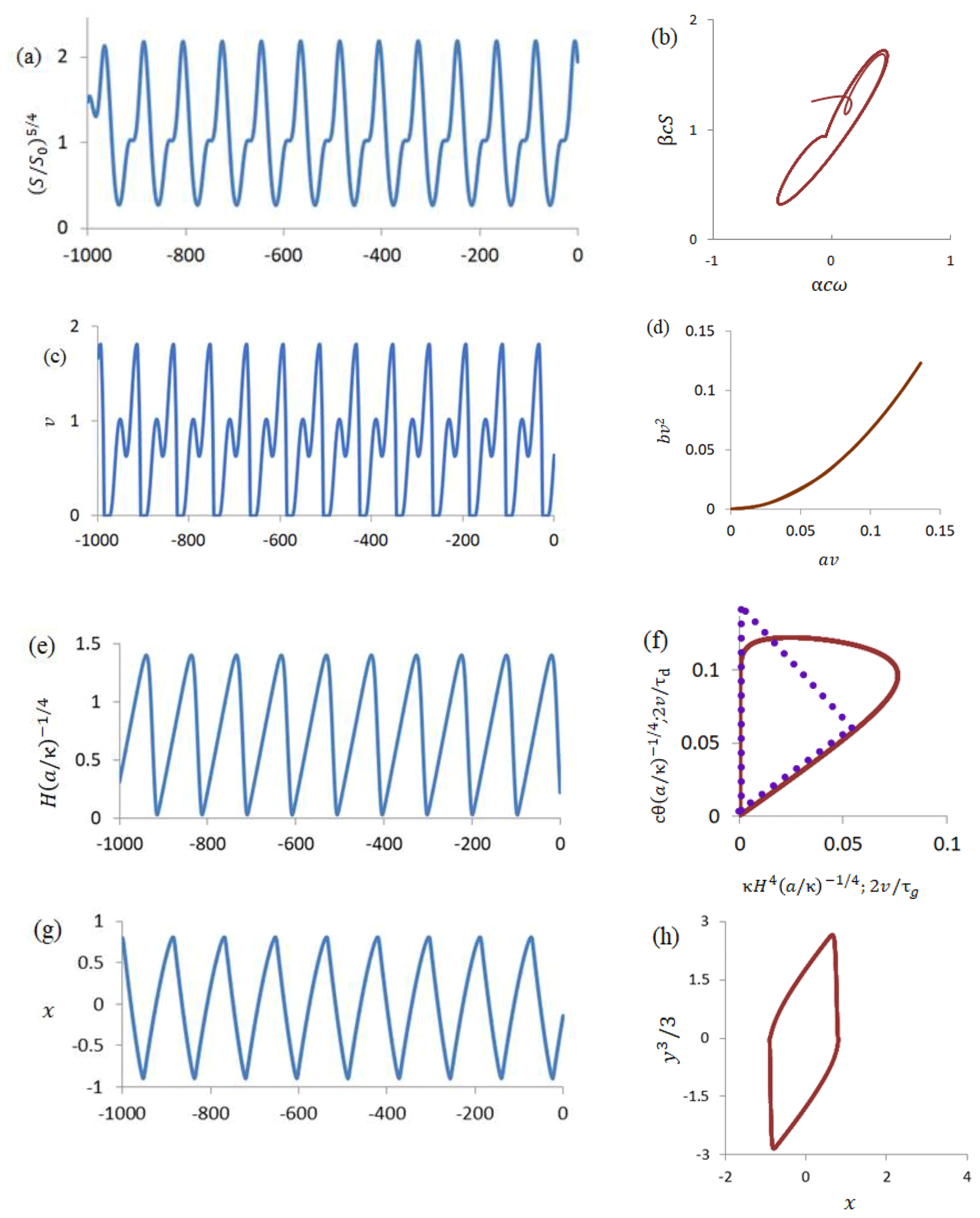
Figure 2Time series (ka) and corresponding positive-versus-negative feedback loops: (a, b) VCV18 (Eqs. 8–10), where is normalized ice volume; (c, d) G23 (Eqs. 12 and 13); (e, f) VCV18-1 (Eqs. 22 and 23), where all variables are normalized by characteristic ice thickness, , and the dotted triangle corresponds to LP22 (Eqs. 44 and 45) without astronomical forcing; and (g, h) VDP (Eqs. 30 and 31).
2.2 G23 model
The G23 model (specifically “Model 2” as annotated in Ganopolski, 2023) describes the evolution of global ice volume v (dimensionless) as a response to orbital forcing εF (F is normalized external forcing of the amplitude ε):
The term δgv* represents an additional positive feedback activated () when . When , . Graphically, the dynamical system (Eqs. 12 and 13) is shown in Fig. 1b. We observe that the dynamics of the G23 system are, like VCV18, defined by the amplitude and periodicity of the orbital forcing, ε, T, and by three feedback loops: two positive feedbacks, av, gv*, and one negative feedback, −bv2. Unlike VCV18, however, all feedbacks are instantaneous. We now review how these differences may be reflected in the corresponding P-scaling law.
For the purpose of dimensional analysis, we consider Eqs. (12) and (13) in dimensional form assuming the following dimensions for variables and parameters involved: t (s), v (m3), a (s−1), b (m−3 s−1), ε (m3 s−1), F (which is a dimensionless function of the period T (s)), d (m3 s−1), δ1, δ2 (dimensionless), g (m−3), and v* (m3). The period of the system response to the astronomical forcing is then a function of the following governing parameters:
For more explicit physical interpretation, instead of the parameter b we will use parameter (m3 s−1), which is the mean growth rate. In addition, for the reference values of parameters provided by G23, d≪ε and δ1, δ2 are constant. Therefore, we can rewrite Eq. (14) as follows:
If we choose , T as parameters with independent dimensions, then according to π theorem
Let us now determine the V number for G23 as the ratio of amplitudes of time-dependent positive and negative feedbacks. Obviously, such a ratio should be completely defined by the internal (terrestrial) G23 properties, giving the following equation:
If we choose a and b as parameters with independent dimensions, then according to π theorem
We can also express g as a function of V:
Accordingly, the P-scaling law of G23 can be written as follows:
or
We see that the scaling law in Eq. 21 is different from the scaling law in Eq. 11 because the Ψ function of Eq. (21) depends on T, unlike the Φ function of Eq. (11). There are only two scenarios for orbital periods to escape the Ψ function (or the Φ function) in a scaling law. First, they may be excluded from the governing equations when the main period of system's variability is attributed to the internal terrestrial physics. This is the case for the VDP and LP22 models that will be considered later, but it is definitely not applicable to either G23 or VCV18. The second scenario occurs when a system incorporates multiple parameters encoding different timescales. The interplay of these parameters may create a situation when T-dependent similarity parameters jointly form a T-independent conglomerate similarity parameter, giving a system the so-called property of incomplete similarity (Barenblatt, 2003). This property has been discovered for VCV18 (Verbitsky, 2022). As the result, the Φ function of the scaling law (Eq. 11) does not depend on orbital period (Φ=2 in the range of T=35–60 kyr). In contrast, as we have already noted, G23 positive and negative feedbacks are instantaneous, the G23 single ice growth timescale does not have a “counterpart” for an interplay, and therefore the Ψ function of Eq. (21) is period T dependent.
Nevertheless, for T=40 kyr, , V=1.1, and Ψ=2 (obliquity period doubling). Hence, only under the obliquity forcing the VCV18 and G23 models appear to be physically similar in regard to two quantitatively close similarity parameters: , the ratio of the astronomical forcing amplitude ε to the growth rate , and the V number. The corresponding time series and positive-versus-negative feedback evolution are shown in Fig. 2c and d. Geometrically, the similarity between the VCV18 and G23 models in terms of the V number emerges from Fig. 2b and d as similar slopes of the corresponding feedback loops; however, the instantaneous nature of G23 feedbacks makes their “loop” asymptotically thin.
2.3 Simplified VCV18 model (VCV18-1) as a proxy for a parent dynamical system
The next phase of our study is devoted to two phenomenological models, VDP and LP22, which have 100 kyr auto-oscillations independent of orbital forcing. To make the diagnostics of physical similarity possible, we have to further simplify VCV18 system with several physically reasonable assumptions.
- a.
Since the global-temperature timescale in Eq. (10) is much faster than other timescales (orbital, ice accumulation, and ice temperature advection), we assume that global temperature is an instantaneous function of the glaciation forcing.
- b.
In Eq. (9), we assume α=0 (for example, the effect of increased global temperature is offset by increased snow precipitation rate; see experiment D in the Appendix of VCV18), which cancels the direct effect of climate on basal temperature.
- c.
We rewrite Eqs. (8) and (9) in terms of ice thickness .
- d.
We attribute all system variability to terrestrial causes (ε=0).
The simplified dynamical system then takes the following form:
The physical meaning of all variables and governing parameters is the same as in Eqs. (8) and (9), but the numerical values and dimensions of some parameters and variables are indeed different – specifically, t (s), H (m), θ (m4), (m s−1), κ (m−3 s−1), and c (m−3 s−1). The casual graph of the dynamical system (Eqs. 22 and 23) is shown in Fig. 1c.
The period of system variability is a function of three governing parameters:
If we choose , κ as parameters with independent dimensions, then according to π theorem
Parameters , κ, c lack in the VDP and LP22 models, and therefore we transition to the V number that must be a function of the same , κ, c parameters:
Since the V number is dimensionless and , κ are parameters with independent dimensions, according to π theorem
This also means that
and we can finally present the VCV18-1 P-scaling law as follows:
In other words, the P-scaling law of the VCV18-1 system is fully defined by the balance between positive and negative feedbacks. For τ=50 kyr, V=0.63 and Φ=2. The corresponding 100 kyr period auto-oscillations of the system (Eqs. 22 and 23) and its positive-versus-negative feedback loop are shown in Fig. 2e and f.
2.4 VDP model
We now consider the VDP model, which is a variant of the historical van der Pol (1922) model used by De Saedeleer et al. (2013) and Crucifix (2013) to study synchronization properties of ice ages.
Here all variables and parameters, except time and timescale τ, are dimensionless. Variable x is a proxy for the glaciation, and variable y represents the rest of the climate. Since , for longer, glaciation-like processes, we can rewrite Eqs. (30) and (31) as follows:
Equation (33) defines the “critical manifold” (Guckenheimer et al., 2003). The system (Eqs. 32 and 33) describes VDP “slow” dynamics between two glacial–interglacial bifurcation points. To get VDP time series, we solve the non-idealized system (Eqs. 30 and 31), and we use the system (Eqs. 32 and 33) to visualize system's positive, x, and negative, , feedbacks. Schematically, the dynamical system (Eqs. 30 and 31) is shown in Fig. 1d. The period of system (Eqs. 32 and 33) variability is the function of two governing parameters:
Only parameter τ is dimensional, and therefore according to π theorem
The amplitudes of VDP variables are defined by the critical manifold (Eq. 33) that does not contain parameters τ, β, and therefore both x and y amplitudes do not depend on model parameters. Consequently, the amplitudes of positive and negative feedbacks do not depend on them either. In fact, the x amplitude in VDP model is always ∼0.8, while the y amplitude is always 2. Therefore, the ratio of the amplitude of the positive feedback, x, to the amplitude of the negative feedback, , is always V=0.3. In summary,
This property (Eq. 36) makes the VDP model fundamentally different from all other models in this study. In all other models, the V number is the function of model's governing parameters, and under different scenarios it changes when parameters change. In the VDP model, the V number is predefined by the model's structure. Consequently, the scaling law (Eq. 35) does not contain any V number, and thus it cannot match the scaling law (Eq. 29). Therefore, there is no physical similarity between the VCV18-1 and the VDP models.
The auto-oscillations of the system (Eqs. 30 and 31) and positive-versus-negative feedback evolution are shown in Fig. 2g and h. For τ=50 kyr and β=0.3, Ψ=2.2. Figure 2e and g show well why the phenomenological approach may be misleading. For the same internal timescale of 50 kyr, VCV18-1 and VDP models both produce asymmetrical (slow growth and fast retreat) glaciation time series with the respective periods P close to 100 kyr, but this occurs because of very different physics: in the VDP model the positive feedbacks are much weaker (V=0.3) than in the VCV18-1 model (V=0.63). Most importantly, this discrepancy cannot be changed because the VDP model is rigid in this regard.
2.5 LP22 model
The LP22 model is described by two differential equations, first, for the growing ice volume,
and another for the diminishing ice volume,
Here, v and I are normalized ice volume and astronomical forcing, respectively, and τi, τg, and τd are dimensional timescales. Additionally, if I<I0 the system switches from Eqs. (38) to (37), while if the system switches from Eq. (37) to (38). Though the original LP22 model does not consider its evolution without astronomical forcing, oscillations still occur when I=0 and the equation-switching conditions are v≤V1 (V1 is the minimal, interglacial, volume) and v≥V0, respectively. Schematically, the dynamical system (Eqs. 37 and 38) with I=0 is shown in Fig. 1e. The period of auto-oscillations is a function of four parameters:
The parameter V1≪V0 can be settled as a constant, and therefore
If we select τg as an independent-dimension parameter, then according to π theorem
Equation (37) describes a linear ice volume growth, implying zero net feedback. This does not indicate the absence of feedbacks. Indeed, if we are ready to accept that the LP22 model is more than just a successful fit to empirical data, then for the growing ice sheet Eq. (37) should be consistent with the dimensional total mass balance
i.e., changes in ice volume are equal to mass influx accumulated over its area S. If we multiply and divide by ice thickness H, the total mass balance (Eq. 42) becomes
where . Equation (43) tells us that the positive feedback must be present in the growing ice sheet: it relates to the area growth with volume. Its absence in Eq. (37) therefore suggests that has another component that completely compensates for and yet another component that is inversely proportional to S (e.g., continentality effect). Hence, the system (Eqs. 37 and 38) must be written as follows to have physical meaning:
Schematically, the dynamical system (Eqs. 44 and 45) is shown in Fig. 1f. The amplitude of the positive feedback is , and the amplitude of the negative feedback is . Since τg>τd, the V number is therefore equal to
Accordingly, the P-scaling law (Eq. 41) for the LP22 model can be written as
For example, for τg=50 kyr, V0=1.5, V1=0.2, and τd=20 kyr, we get V=0.4 and Ψ=2, and, as we have established before, for the VCV18-1 model, τ=50 kyr, V=0.63, and Φ=2. Therefore, we can talk about physical similarity between the VCV18-1 and LP22 models in terms of reasonably close V numbers.
The similarity between the VCV18-1 and LP22 models becomes very visual in Fig. 2f, which describes the positive-versus-negative feedback loops. It can be observed during much of the ice growth in the VCV18-1 model that positive and negative feedbacks also completely compensate for each other. In fact, we can consider the LP22 model to be an approximation of the VCV18-1 feedback loop by a triangle. Indeed, the LP22 positive and negative feedbacks compensate for each other during ice advance, and when the critical value of v (i.e., V0) is achieved, the system instantly migrates to the single dominant negative feedback. Simply put, these two models are as similar to one another as the shape of the LP22 feedback loop triangle in Fig. 2f is similar to the shape of the VCV18-1 feedback loop, as the V number is the ratio of its horizontal dimension to its vertical dimension. This similarity can be illustrated even further if we compare explicit scaling laws (Eqs. 29 and 47). For this purpose, we solved equations (Eqs. 22 and 23) by changing the parameter c and thus gradually changing the balance between positive and negative feedbacks. The results of these additional experiments are presented in Fig. 3 together with the P-scaling law (Eq. 47) that can be estimated in a very straightforward manner: or , which is finally . It can be observed that the LP22 scaling law closely resembles the VCV18-1 scaling law trend line, thus supporting our assertion that we can consider the LP22 model being an approximation of the VCV18-1 model.
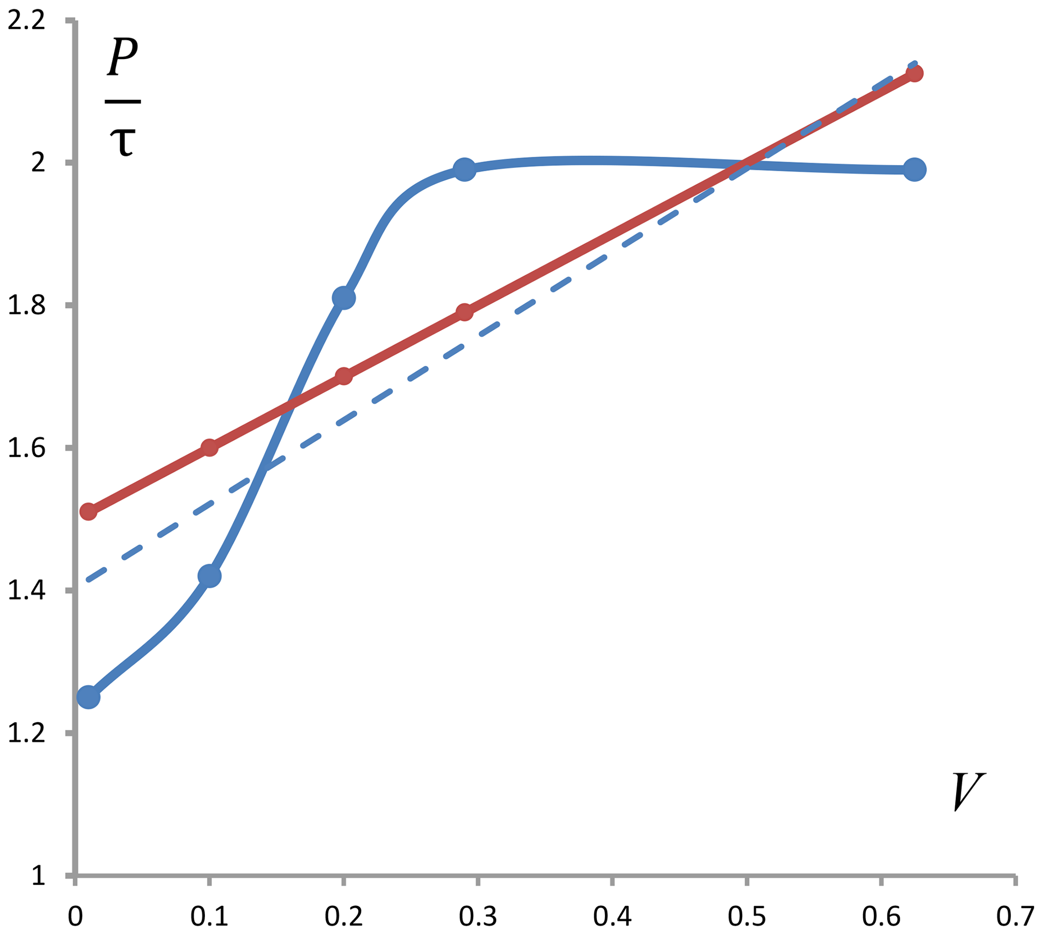
Figure 3The P-scaling laws of the VCV18-1 (blue; the dotted line is its trend line) and the LP22 (brown) model.
Nikolai Gogol would have said that “a magic apple tree may grow golden apples … but not pears”. Phenomenological models may not be bounded by a specific physics, but they have to be consistent with the laws of physics. The concept of physical similarity is what allows us to be vigilant about such consistency. Accordingly, we started our presentation with the following question: are phenomenological dynamical paleoclimate models physically similar to Nature? We demonstrated that though they may be remarkably accurate in reproducing empirical time series, this is not sufficient to claim physical similarity with Nature until similarity parameters are considered. We illustrated such a process of diagnostics of physical similarity by comparing three phenomenological dynamical paleoclimate models with the more explicit model that played the role of a parent dynamical system. Though the nomination of the VCV18 model to serve as a proxy for the parent dynamical system can indeed be questioned and the developments of better proxies should be encouraged, we nevertheless believe that the diagnostics of physical similarity we have described should become a standard procedure before a phenomenological model can be utilized for interpretations of historical records or for future predictions. In other words, claiming a model to be a phenomenological one is not an indulgence but a liability.
The results of the analysis are summarized in Fig. 4. Here, the physical similarity is visualized as the proximity between the models in the space.
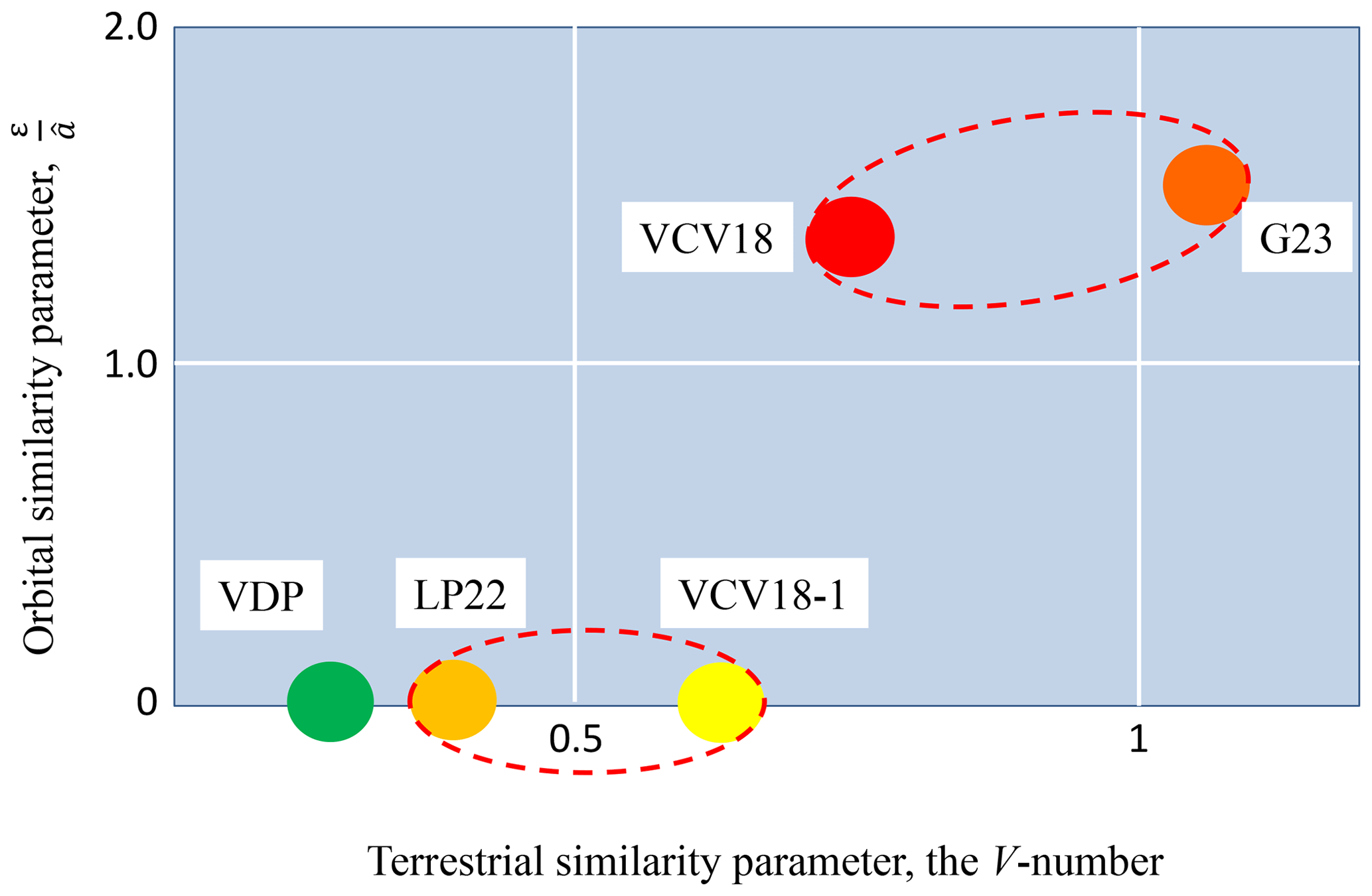
Figure 4Physical similarity diagnostics for the obliquity period doubling of the VCV18 and G23 models and for 100 kyr auto-oscillations of the VDP, LP22, and VCV18-1 models. The physical similarity is visualized here as proximity between the models in the space. Dashed red ovals embrace models that we found to be physically similar, and therefore they are in reasonably close proximity in the diagram.
LP22 and G23 models can be considered to be physically similar to particular versions of the VCV18 model, which amounts to saying that they may be derived from basic laws of physics under some reasonable physical assumptions. These findings boost the physical viability of these phenomenological models, but this is not unconditional and there are clear boundaries to the physical legitimacy of these phenomenological models. For LP22, the ratio of the feedback's amplitudes, the V number, is also the ratio of the timescales. For the Late Pleistocene and the Early Pleistocene, all timescales are likely to be different, and the physical similarity would therefore need to be re-examined separately for each period. For the G23 model, physical similarity was found only for the obliquity range forcing.
Generally speaking, our observation that the VDP model is not physically similar to the simplified version of the VCV18 model is not a final verdict. It is indeed an indication that VDP is not based on ice physics, but there may be other physical phenomena that may provide physical legitimacy to the VDP model. We are, however, a bit skeptical that such a phenomenon can easily be found because it would need to be constrained in the same way as the VDP model. Specifically, its ratio of positive and negative feedbacks must to be fixed to a specific value that never changes.
Figure 4 clearly shows that the VDP, LP22, and even VCV18-1 models are not physically similar to the VCV18 model. Indeed, the VDP, LP22, and VCV18-1 scaling laws do not have a similarity parameter that is a ratio of orbital and terrestrial forcing amplitudes, and therefore these models are located on the horizontal axis of Fig. 4. Interestingly, the VDP, LP22, and VCV18-1 models are located to the left of the VCV18 and G23 models, thus revealing the more prominent role of their negative feedbacks. As is clearly displayed in the positive-versus-negative feedback diagrams of Fig. 2, this happens because the mechanism of ice disintegration in these two groups of models is based on very different physics. In the VCV18-1, VDP, and LP22 models, the disintegration of ice sheets happens when the negative feedback suddenly becomes dominant and destroys an ice sheet. In both the VCV18 and G23 models, the disintegration is due to the additional fast positive feedback, which is small during most of the ice growth period but eventually becomes strong enough to boost the orbital forcing that attempts ice destruction.
Importantly, we arrived at the above conclusions without making any effort to somehow artificially minimize (or maximize) a “distance” between the models in Fig. 4 (though it may be an interesting separate exercise) but instead for the most part used published reference values of model parameters.
In addition, it should not be forgotten that Fig. 4 is just our attempt to present the most important results visually in one diagram. Since it is 2-dimensional, it demonstrates similarity (or its absence) in terms of two similarity parameters, the ratio of astronomical forcing amplitude to the terrestrial growth rate and the positive-to-negative feedback ratio. These two dimensions would not be sufficient if more similarity parameters need to be visually presented. For example, Eq. (21) shows that the G23 model depends on the similarity parameter formed by the ratio of the orbital period T to the internal timescale . This similarity parameter is absent in the VCV18 model. This absence of similarity is not apparent from Fig. 4, but it is discussed in Sect. 2.2.
As a final conclusion, we agree with the Saltzman (2002) proposal that “the essential slow physics is to be sought in the low-order models.” We observe, however, that “essential slow physics” that can be derived from phenomenological models is limited to orbital and terrestrial timescales, to ratios of amplitudes of orbital and terrestrial forcings, and to ratios of amplitudes of positive and negative feedbacks. This is as much as phenomenological models can offer, and therefore we deviate from further idea of Saltzman (2002) that more explicit models should be tuned to satisfy a best phenomenological model. Instead, we propose using available physical models for diagnostics of the physical-similarity hypothesis that need to be either confirmed or rejected. Specifically, physical models have to be explored to identify additional dimensionless quantities playing key roles in their dynamics. Further, finding values for these quantities should be a central objective of future research into glacial–interglacial dynamics.
Of course, encoding empirical data in a simple mathematical statement will always remain a tempting possibility. As Grigory Barenblatt (2003) said, “applied mathematics is the art of constructing mathematical models of phenomena in nature”. This means that there are no strict rules as to how a piece of mathematical “art” needs to be produced. Therefore, we do not attempt here to discourage our fellow “artists” from alluding to phenomenological models. Our goal instead was to remind them about the limitations of phenomenological models and to suggest how these limitations may be addressed.
The MATLAB R2015b code and data to reproduce the time series and corresponding feedback loops as they are presented in Fig. 2 are available at https://doi.org/10.5281/zenodo.8329443 (Verbitsky, 2023).
This paper refers exclusively to published research articles and their data. We refer the reader to the cited literature (Berger and Loutre, 1991) for access to data.
MYV conceived the research, developed the formalism, and wrote the first draft of the manuscript. The authors jointly discussed the findings and contributed equally to the editing of the manuscript.
The contact author has declared that neither of the authors has any competing interests.
Publisher's note: Copernicus Publications remains neutral with regard to jurisdictional claims in published maps and institutional affiliations.
We are grateful to Andrey Ganopolski for discussions and generous insight into the G23 model, including the time series of Fig. 2c and d, and to Dmitry Volobuev for his help in digitizing VCV18. We are also grateful to our two anonymous reviewers for their helpful suggestions.
This paper was edited by Z. S. Zhang and reviewed by two anonymous referees.
Barenblatt, G. I.: Scaling, Cambridge University Press, Cambridge, ISBN 0521533945, 2003.
Berger, A. and Loutre, M. F.: Insolation values for the climate of the last 10 million years, Quaternary Sci. Rev., 10, 297–317, 1991.
Buckingham, E.: On physically similar systems; illustrations of the use of dimensional equations, Phys. Rev., 4, 345–376, 1914.
Crucifix, M.: Why could ice ages be unpredictable?, Clim. Past, 9, 2253–2267, https://doi.org/10.5194/cp-9-2253-2013, 2013.
De Saedeleer B., Crucifix, M. and Wieczorek, S.: Is the astronomical forcing a reliable and unique pacemaker for climate? A conceptual model study, Clim. Dynam., 40, 273–294, https://doi.org/10.1007/s00382-012-1316-1, 2013.
Ganopolski, A.: Toward Generalized Milankovitch Theory (GMT), Clim. Past Discuss. [preprint], https://doi.org/10.5194/cp-2023-57, in review, 2023.
Guckenheimer, J., Hoffman, K., and Weckesser, W.: The Forced van der Pol Equation I: The Slow Flow and Its Bifurcations, SIAM J. Appl. Dynam. Syst., 2, 1–35, https://doi.org/10.1137/S1111111102404738, 2003.
Haken, H.: Information and self-organization: A macroscopic approach to complex systems, Springer Science & Business Media, ISBN 3-540-66286-3, 2006.
Kaufmann, R. K., and Pretis, F.: Understanding glacial cycles: A multivariate disequilibrium approach, Quaternary Sci. Rev., 251, 106694, https://doi.org/10.1016/j.quascirev.2020.106694, 2021.
Leloup, G. and Paillard, D.: Influence of the choice of insolation forcing on the results of a conceptual glacial cycle model, Clim. Past, 18, 547–558, https://doi.org/10.5194/cp-18-547-2022, 2022.
Paillard, D.: The timing of Pleistocene glaciations from a simple multiple-state climate model, Nature, 391, 378–381, 1998.
Saltzman, B.: Dynamical paleoclimatology: generalized theory of global climate change, in: Vol. 80, Academic Press, San Diego, CA, ISBN 0126173311, 2002.
Saltzman, B. and Maasch, K. A.: A first-order global model of late Cenozoic climatic change II. Further analysis based on a simplification of CO2 dynamics, Clim. Dynam., 5, 201–210, 1991.
Saltzman, B. and Verbitsky, M. Y.: Asthenospheric ice-load effects in a global dynamical-system model of the Pleistocene climate, Clim. Dynam., 8, 1–11, 1992.
Saltzman, B. and Verbitsky, M. Y.: Multiple instabilities and modes of glacial rhythmicity in the Plio-Pleistocene: a general theory of late Cenozoic climatic change, Clim. Dynam., 9, 1–15, 1993.
Saltzman, B. and Verbitsky, M.: Late Pleistocene climatic trajectory in the phase space of global ice, ocean state, and CO2: Observations and theory, Paleoceanography, 9, 767–779, 1994.
Talento, S. and Ganopolski, A.: Reduced-complexity model for the impact of anthropogenic CO2 emissions on future glacial cycles, Earth Syst. Dynam., 12, 1275–1293, https://doi.org/10.5194/esd-12-1275-2021, 2021.
Tzedakis, P. C., Crucifix, M., Mitsui, T., and Wolff, E. W.: A simple rule to determine which insolation cycles lead to interglacials, Nature, 542, 427–432, 2017.
Tziperman, E., Raymo, M. E., Huybers, P., and Wunsch, C.: Consequences of pacing the Pleistocene 100 kyr ice ages by nonlinear phase locking to Milankovitch forcing, Paleoceanography, 21, PA4206, https://doi.org/10.1029/2005PA001241, 2006.
van der Pol, B.: On oscillation hysteresis in a triode generator with two degrees of freedom, Philos. Mag. Ser., 6, 700—719, https://doi.org/10.1080/14786442208633932, 1922.
Verbitsky, M. Y.: Inarticulate past: similarity properties of the ice–climate system and their implications for paleo-record attribution, Earth Syst. Dynam., 13, 879–884, https://doi.org/10.5194/esd-13-879-2022, 2022.
Verbitsky, M. Y.: Supplementary code and data to Climate of the Past paper “Do phenomenological dynamical paleoclimate models have physical similarity with Nature? Seemingly, not all of them do” by Mikhail Y. Verbitsky and Michel Crucifix, Zenodo [code], https://doi.org/10.5281/zenodo.8329443, 2023.
Verbitsky, M. Y. and Chalikov, D. V.: Modelling of the Glaciers-Ocean-Atmosphere System, edited by: Monin, A. S., Gidrometeoizdat, Leningrad, 135 pp., 1986.
Verbitsky, M. Y. and Crucifix, M.: π-theorem generalization of the ice-age theory, Earth Syst. Dynam., 11, 281–289, https://doi.org/10.5194/esd-11-281-2020, 2020.
Verbitsky, M. Y. and Crucifix, M.: ESD Ideas: The Peclet number is a cornerstone of the orbital and millennial Pleistocene variability, Earth Syst. Dynam., 12, 63–67, https://doi.org/10.5194/esd-12-63-2021, 2021.
Verbitsky, M. Y., Crucifix, M., and Volobuev, D. M.: A theory of Pleistocene glacial rhythmicity, Earth Syst. Dynam., 9, 1025–1043, https://doi.org/10.5194/esd-9-1025-2018, 2018.