the Creative Commons Attribution 4.0 License.
the Creative Commons Attribution 4.0 License.
 | 27 Jul 2023
The challenge of comparing pollen-based quantitative vegetation reconstructions with outputs from vegetation models – a European perspective
Anne Dallmeyer
Anneli Poska
Laurent Marquer
Andrea Seim
Marie-José Gaillard
We compare Holocene tree cover changes in Europe derived from a transient Earth system model simulation (Max Planck Institute Earth System Model – MPI-ESM1.2, including the land surface and dynamic vegetation model JSBACH) with high-spatial-resolution time slice simulations performed in the dynamic vegetation model LPJ-GUESS (Lund–Potsdam–Jena General Ecosystem Simulator) and pollen-based quantitative reconstructions of tree cover based on the REVEALS (Regional Estimates of Vegetation Abundance from Large Sites) model. The dynamic vegetation models and REVEALS agree with respect to the general temporal trends in tree cover for most parts of Europe, with a large tree cover during the mid-Holocene and a substantially smaller tree cover closer to the present time. However, the decrease in tree cover in REVEALS starts much earlier than in the models, indicating much earlier anthropogenic deforestation than the prescribed land use in the models. While LPJ-GUESS generally overestimates tree cover compared to the reconstructions, MPI-ESM indicates lower percentages of tree cover than REVEALS, particularly in central Europe and the British Isles. A comparison of the simulated climate with chironomid-based climate reconstructions reveals that model–data mismatches in tree cover are in most cases not driven by biases in the climate. Instead, sensitivity experiments indicate that the model results strongly depend on the tuning of the models regarding natural disturbance regimes (e.g. fire and wind throw). The frequency and strength of disturbances are – like most of the parameters in the vegetation models – static and calibrated to modern conditions. However, these parameter values may not be valid for past climate and vegetation states totally different from today's. In particular, the mid-Holocene natural forests were probably more stable and less sensitive to disturbances than present-day forests that are heavily altered by human interventions. Our analysis highlights the fact that such model settings are inappropriate for paleo-simulations and complicate model–data comparisons with additional challenges. Moreover, our study suggests that land use is the main driver of forest decline in Europe during the mid-Holocene and late Holocene.
- Article
(11209 KB) - Full-text XML
- BibTeX
- EndNote


Terrestrial land cover is one of the key components of the Earth's ecosystem and a provider of many ecosystem services. It is widely discussed in the context of ongoing climate change due to its high sensitivity to environmental changes and its role as one of the mitigation agents of the current and projected global warming (e.g. Williamson, 2016; Harper et al., 2018; Smith et al., 2016). Decisions on strategies for the future depend, among others, on our ability to correctly understand the interactions between vegetation and climate over short and millennial timescales. This also requires that Earth system models (ESMs) correctly simulate these interactions in the past to ensure reliable model projections (Harrison et al., 2020). In this context, dynamic global vegetation models (DGVMs) are used, either coupled to ESMs or offline, to simulate past or future climate- and human-induced changes in land cover composition, biomass production, and carbon storage capacity (e.g. Hickler et al., 2012; Wramneby et al., 2010; Hopcroft et al., 2017; Lu et al., 2018, 2021). However, the DGVM parameterizations (bioclimatic limits, disturbance intervals, fire regimes, etc.) are commonly static and based on the current state of land cover although they are characterized by unstable vegetation composition due to rapidly changing natural and anthropogenic stressors (Hengl et al., 2018). This is one of several caveats of DGVMs that may lead to erroneous projections for the future.
Comparison of DGVM simulations for the past with proxy records of vegetation composition is a way to evaluate the performance of DGVMs. Among existing empirical proxies of past vegetation, pollen records from lake sediments or peat deposits have the best potential for quantitative reconstructions of plant abundance or spatial cover. However, pollen records are subject to several shortcomings such as unknown size of the source area of pollen and differences in pollen productivity and dispersal properties between plant taxa (e.g. Prentice, 1985). These issues imply that pollen percentages (and pollen accumulation rates) from fossil pollen assemblages can only provide qualitative or semi-quantitative information on past vegetation changes, i.e. sporadic or regular presence, occurrence in more or less large quantities, and increases and decreases in abundance of plant taxa. Different methods have been developed to overcome these problems and reconstruct plant cover, e.g. biomization, the modern analogue technique (MAT), pseudo-biomization, and the landscape reconstruction algorithm (REVEALS and LOVE models). These methods are described and evaluated in e.g. Hellman et al. (2008a) and Roberts et al. (2018).
REVEALS (Regional Estimates of Vegetation Abundance from Large Sites) (Sugita, 2007) is the only method so far that accounts for inter-taxonomic differences in pollen productivity as well as dispersal and deposition properties and provides estimates of plant cover (in % cover of a defined area) for individual taxa. In recent years, datasets of pollen-based REVEALS plant cover were produced at a 1∘ grid cell spatial scale for large regions of the world, i.e. Europe, China, and North America–Canada (Trondman et al., 2015; Marquer et al., 2017; Dawson et al., 2018; Cao et al., 2019; Githumbi et al., 2022a; Li et al., 2023; Serge et al., 2023). These datasets are appropriate for use in paleoclimate modelling (e.g. Strandberg et al., 2022, 2023) and evaluation of dynamic vegetation models (e.g. Marquer et al., 2017, 2018) as well as scenarios of anthropogenic land cover change (e.g. Kaplan et al., 2017).
Europe is a good test bed for model evaluation because it offers a dense network of pollen records and thus many pollen-based reconstructions of regional plant cover at semi-continental and continental scales (Trondman et al., 2015; Marquer et al., 2014, 2017; Githumbi et al., 2022a; Serge et al., 2023). Moreover, these reconstructions were successfully combined with auxiliary datasets (four covariates: latitude, longitude, elevation, independent scenarios of past deforestation) to create spatially continuous maps for 6 ka (Pirzamanbein et al., 2014, 2020) and continuous time windows from 11.7 ka to the present (Githumbi et al., 2022b) using spatial statistical models.
Pollen analyses indicate large changes in plant species composition and distribution over the Holocene. They represent both natural and human-induced (land use) changes, the latter increasing gradually from 6 ka until today. Such human-induced land cover changes could potentially have a large impact on complex climate–vegetation interactions and represent a significant climate forcing in the past (Ruddiman et al., 2015; Ruddiman, 2007; Boy et al., 2022; Huang et al., 2020). Regional climate model simulations have shown that the anthropogenic deforestation of Europe at 6 ka according to the KK10 scenarios (Kaplan et al., 2009) and the pollen-based land cover reconstructions of Githumbi et al. (2022a) result in regional cooling or warming of 1 ∘C depending on the region and season (Strandberg et al., 2014, 2022)
An earlier evaluation of the performance of the DGVM LPJ-GUESS (Lund–Potsdam–Jena General Ecosystem Simulator) by comparing model-simulated land cover with pollen-based plant cover reconstructions in Europe showed clear differences between the two for the first 1 to 2 millennia of the Holocene and over the last 7000–6000 years (e.g. Marquer et al., 2017, 2018). The largest discrepancies are found in the abundance and cover of open land, with LPJ-GUESS generally underestimating the extent of unforested land. While model–data mismatches are commonly associated with biases in climate inputs (Strandberg et al., 2022), an increasing amount of evidence shows good conformity between climate model outputs and climate reconstructions inferred from proxies other than pollen. It implies that mismatches are rather related to the lagged reaction of trees to climate change (Dallmeyer et al., 2022) and the increasing effect of anthropogenic land cover change in Europe from 6000 years ago (Kleinen et al., 2011; Braconnot et al., 2019).
The aim of this study is to explore the mechanisms behind discrepancies between DGVM-simulated and empirically reconstructed (pollen-based) plant abundance and distributions. We compare tree cover changes simulated by two commonly used DGVMs with different inherent vegetation representation and parameterization, the Max Planck Institute Earth System Model (MPI-ESM1.2) land model component JSBACH and the DGVM LPJ-GUESS, with empirical pollen-based REVEALS plant cover reconstructions for six time windows of the Holocene and five areas along S–N and W–E transects through central and northern Europe. Both model-simulated and pollen-reconstructed plant cover is expressed in percentage cover of a known area. Henceforth, all ages are given in calibrated 14C kilo years BP, abbreviated “ka”.
In this study, we use DGVMs with very different modelling approaches. JSBACH is the land surface component of the comprehensive Earth system model MPI-ESM and thus interactively calculates the grid cell cover fractions of different plant functional types (PFTs) in line with the simulated climate (Reick et al., 2021). In contrast, LPJ-GUESS is a so-called “gap” model that calculates the growth of individuals or cohorts in patches, according to a prescribed climatic forcing (Smith et al., 2001). While we explore one of the few transient Holocene Earth system model simulations (MPI-ESM) available worldwide, high-spatial-resolution time slice experiments in LPJ-GUESS have been conducted in this study. LPJ-GUESS is used here because it is well-tested for the European domain (e.g. Hickler et al., 2012). The results of both models are compared to the pollen-based REVEALS reconstructions of plant cover for Europe from Marquer et al. (2017). These reconstructions were chosen before others based on other methods such as MAT (e.g. Davis et al., 2015) or pseudo-biomization (e.g. Fyfe et al., 2010) because the REVEALS model has been shown to be the best approach to produce reliable quantitative reconstructions of forest cover and the only method available to date to reconstruct the cover of individual plant taxa (e.g. Hellman et al., 2008a; Roberts et al., 2018; see also Sect. 1 above). The methodological strategy used in this study is summarized in the flowchart in Fig. 1.
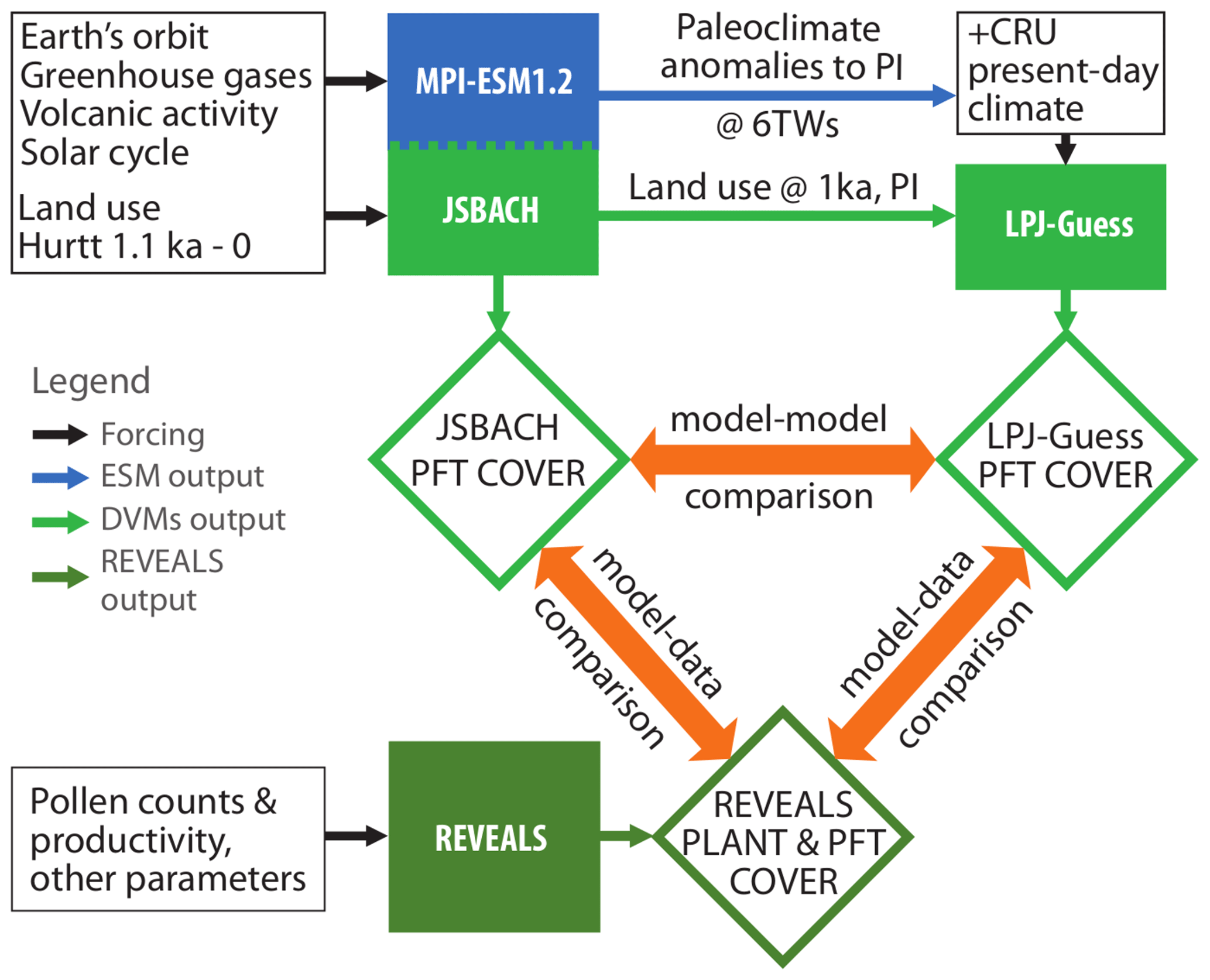
Figure 1Flowchart of the strategy for the comparison between the plant functional type (PFT) cover simulated by the dynamic global vegetation models JSBACH (interactively coupled in the Earth system model MPI-ESM1.2) as well as LPJ-GUESS (stand-alone model) and the pollen-based REVEALS plant cover reconstructions. The MPI-ESM1.2 simulation and the REVEALS-based reconstructions have been published earlier in Bader et al. (2020) and Marquer et al. (2019), respectively. Within this study, LPJ-GUESS simulations for six different time windows (TWs) were performed and compared with the MPI-ESM1.2 results and REVEALS reconstructions. As land use forcing for JSBACH, a preliminary version of the LUH2 dataset by Hurtt et al. (2020) was used. The climate and land use forcings for LPJ-GUESS were extracted from the output of the MPI-ESM1.2 model, but to overcome temperature biases due to the coarse spatial resolution, the MPI-ESM-simulated climate anomalies to PI were interpolated bilinearly to a grid and added to the observational CRU dataset (Harris et al., 2020) before prescribing them to LPJ-GUESS.
2.1 The Earth system model MPI-ESM1.2 transient simulation
We use the existing transient simulation for the period 7.95–0.1 ka conducted by Bader et al. (2020) in the Max Planck Institute Earth System Model (MPI-ESM, version 1.2) (Mauritsen et al., 2019). This simulation has been forced by changes in insolation (Berger, 1978), greenhouse gas concentrations (Fortunat Joos, personal communication, 2016; see Köhler, 2019 and Brovkin et al., 2019), stratospheric sulfate aerosol injections imitating volcanic eruptions (Toohey and Sigl, 2017), spectral solar irradiance (Krivova et al., 2011), and human-induced land cover changes (preliminary version of Hurtt et al., 2020). The atmosphere and land model were applied with a spectral resolution of T63 (approx. 200 km on a Gaussian grid). While the simulation and forcing mechanisms were described in detail in earlier studies (Bader et al., 2020; Brovkin et al., 2019; Dallmeyer et al., 2020), we focus here only on the dynamic vegetation calculation and the land use forcing.
MPI-ESM includes the land surface model JSBACH with the dynamic vegetation module developed by Brovkin et al. (2009). In this module, natural vegetation is represented by eight plant functional types (PFTs). Trees (four PFTs) can be either tropical or extratropical (i.e. boreal + temperate) and evergreen or deciduous. The open land cover is represented by two herbaceous PFTs (C3 and C4 grass) and two shrub PFTs (raingreen shrubs and cold-resistant shrubs). Land use (anthropogenic vegetation) is included as three PFTs (i.e. C3 pasture, C4 pasture, and crops). Therefore, total plant cover is represented by 11 PFTs (see details on the implementation of anthropogenic PFTs below). Different PFTs can coexist in each grid cell as the model uses a tiling approach; i.e. the grid cell is tiled in mosaics of fractional PFT coverages. The establishment of each natural PFT is constrained by temperature thresholds representing their respective bioclimatic tolerance. The fractional cover of each PFT is, by and large, determined by the relative differences in annual net primary productivity (NPP) between the PFTs. Natural mortality and disturbances, such as wind throw and fire, reduce the cover fraction of PFTs. Woody PFTs are generally favoured at the expense of grass, but in regions with frequent disturbances or bioclimatic conditions near the bioclimatic thresholds, shrubs or even grass may win the competition as they can recover more quickly than trees. The relative presence of grasses and woody PFTs is thus implicitly determined by the strength of the disturbances. While fire has a different effect on grass than on woody PFTs, wind throw only reduces the woody PFT types. The disturbance rate of wind throw is proportional to the simulated wind power, but it is weighted by the averaged wind speed in each grid cell to account for the adaptation of woody plants to local wind conditions. In addition, wind throw is set to zero if wind speeds are below a threshold that is determined by the long-term average maximum wind speed.
For each grid cell, JSBACH calculates the fraction of the grid cell that is not covered by vegetation (bare soil fraction) that represents both seasonal and permanently unvegetated ground. Since the area of bare soil cannot be estimated by the REVEALS model (see Sect. 2.3), the PFT fractions in this study are scaled based on the total area covered by vegetation; i.e. the bare soil fraction is not considered and the cover fractions of the PFTs are adjusted to sum up to 1 in each grid cell.
Human-induced land cover changes affect the simulation only for the last ∼2000 years. In the simulation, the anthropogenic land cover changes have been prescribed from a preliminary version of the Land-Use Harmonization 2 dataset (LUH2) (Hurrt et al., 2020). This dataset provides the land use changes for the 850 CE to 2100 CE period and could therefore only be used as forcing of the model for the last 1000 years of the transient simulation (from 1.1 ka on). To slowly build up the land use in the course of the simulation from zero to the anthropogenically influenced land cover at 1.1 ka, a transition period of 1000 years has been implemented starting at 2.1 ka. Land use is read annually but calculated daily by linear interpolation. Land use is prescribed in the form of transition maps that define the fraction of area that is converted from natural vegetation to crops and pasture or vice versa. Pasture is first distributed in the area covered by grass before it replaces forested area (Reick et al., 2021). After this rule has been applied, the remaining anthropogenic land cover change is equally distributed to all PFTs, relative to their individual cover fractions, in order to have the same gain or loss of cover fraction.
More details on the dynamic vegetation module can be found in Brovkin et al. (2009) and Reick et al. (2013, 2021). An evaluation of the simulated pre-industrial (PI) climate is provided in Appendix A.
2.2 The LPJ-GUESS simulated plant cover
2.2.1 Model description
LPJ-GUESS (Lund–Potsdam–Jena General Ecosystem Simulator) is an individual-based dynamic ecosystem model optimized for global to regional studies (Smith et al., 2001, 2014; Sitch et al., 2003). The model employs a representation of vegetation dynamics (successional processes: establishment, growth, mortality) of a forest “gap” model allowing explicit representation of competition for resources (light, water, nutrients, etc.). Growth of individuals or cohorts is simulated in several replicate patches of 0.1 ha representing the grid cell. The climatic conditions and soil type are assumed to be identical between the patches. The probability of stochastic patch-destroying disturbance (fire, wind, etc.) occurrence is controlled by pre-set generic disturbance intervals. When disturbances occur, the vegetation cover of the one patch is destroyed. The proportion of vegetation affected is dependent on the total number of prescribed patches. The vegetation is simulated as PFTs discriminated in terms of bioclimatic limits and physiological characteristics. The standard global PFT set comprises 10 woody PFTs representing major higher plant types of boreal, temperate, and tropical biomes and two grass PFTs distinguished by C3 and C4 photosynthetic pathways. Land use is implemented using external inputs determining the proportional distribution of up to seven land cover types (natural vegetation, urban areas, cropland, managed forest, pastureland, peatland, and barren land) and an associated specialized PFT set to simulate the land cover dynamics and biogeochemical fluxes (Lindeskog et al., 2013).
The model has been applied and benchmarked in a number of studies for both global and European conditions (Smith et al., 2008; Hickler et al., 2012) as well as agricultural landscapes (Müller et al., 2021; Lindeskog et al., 2013). It is among the best available C cycle models (Piao et al., 2013) and can account for C–N interactions (Smith et al., 2014). Model performance in terms of reproducing vegetation as well as hydrological and biogeochemical cycles for past, present, and future applications has been tested in numerous studies (e.g. Garreta et al., 2010; Miller et al., 2008; Olofsson and Hickler, 2008).
2.2.2 High-resolution time slice simulations with LPJ-GUESS
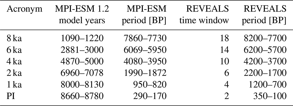
LPJ-GUESS was forced with ca. 120-year monthly resolved climate (total cloud cover, precipitation, and 2 m air temperature) from the transient MPI-ESM1.2 simulation. Model runs were performed for six time slices, four of which are distributed at nearly equal time intervals between 8 and 2 ka (representing the mid-Holocene and late Holocene), and two fall in the period with prescribed land use in the MPI-ESM1.2 simulation. The periods of the input climate data have been selected based on the two criteria of being close to the period of interest (e.g. 8 ka) and showing a relatively stable climate, characterized by few effects of the prescribed volcanic activity in the MPI-ESM1.2 simulation on the regional climate. The age intervals and acronyms of the six time slices are provided in Table 1.
Table 1Overview of selected time slices and their acronyms in this study. The MPI-ESM1.2 periods used as climate forcing for the LPJ-GUESS model are provided in both model years (1001: 7949 BP) and corresponding calibrated 14C years BP. The time windows for the pollen-based REVEALS estimates of regional plant cover follow the standard protocol used in PAGES LandCover6k (Marquer et al., 2019).
To minimize the effect of systematic biases in the simulated climate on LPJ-GUESS-simulated vegetation, an anomaly approach was used (Wohlfahrt et al., 2008). First, the anomaly between each month of each year of a simulated period (e.g. 8 ka) and the respective climatological monthly mean at the end of the simulation (i.e. 0.2–0.1 ka) were calculated based on the original T63 gridded MPI-ESM1.2 output. These anomalies were then interpolated bilinearly to a regular grid with a spatial resolution of and added to a reference climate dataset, i.e. the climatological monthly mean of the years 1901–1930 taken from the University of East Anglia Climatic Research (CRU) TS 4.0 dataset (Harris et al., 2020; University of East Anglia Climatic Research Unit (CRU) et al., 2017). The anomaly approach has the advantage of preserving regional climatic gradients that are an imprint of e.g. complex orography (Harrison et al., 1998) despite the relatively coarse spatial resolution used in the MPI-ESM1.2 simulation. To avoid negative values in precipitation and cloud cover (resulting from the anomaly calculation) in the LPJ-GUESS climate forcing data, all negative values were set to 0 for these variables.
The spin-up to reach vegetation and biogeochemical equilibrium was set to 300 years using the first 30 years of the detrended climate data for the time window. Inputs of monthly climate variables (temperature, precipitation and cloud cover), soil texture data described in Sitch et al. (2003), and land use proportions derived from the JSBACH output (1 ka and PI time slice), along with a set of PFT-specific parameters determining the bioclimatic niche and physiological parameters (growth form, leaf phenology, photosynthetic pathway, life history, etc.), were used to set up the simulation. The number of simulated patches was set to 25 and the disturbance interval to the standard 100 years for all model runs except for the disturbance sensitivity tests. These tests were also run with 25 patches while changing the disturbance interval in each run (25, 75, and 200 years). Each time a disturbance occurred, one patch (i.e. ca. 4 %) of the simulated vegetation was destroyed.
Yearly outputs of the computed PFT-specific leaf area indices (LAIs) per grid cell were recorded. The spatial resolution of the LPJ-GUESS runs matched that of the climate inputs. Simulations ran uninterrupted for the whole time series. The model-produced annual record of PFT-specific LAI was averaged over the last 30 years of the modelled time slice and converted to fractional plant cover (FPC) by applying a simplified version of Lambert–Beer law (Sitch et al., 2003; Monsi and Saeki, 1953; Monsi, 2004; Prentice et al., 1993):
All woody FPC(PFT) fractions were summed to represent total tree cover (TC) of the grid cell, and the grass FPC(PFT) and land-use-related FPC(PFT) (for 1 ka and PI only) were summed to represent the total open land cover (OC) fraction. To ensure comparability with pollen-based vegetation cover estimates (i.e. assuming 100 % vegetation cover), the model-based TC and OC were recalculated to sum up to 100 % cover in each grid cell.
2.3 Pollen-based REVEALS plant cover reconstructions
2.3.1 The REVEALS model
The REVEALS model was developed to estimate regional plant abundance using pollen count records from large lakes (>50 ha) and corrects for the biases due to inter-taxonomic differences in pollen productivity, dispersal, and deposition (Sugita, 2007). REVEALS can also be applied with pollen records from multiple small sites (lakes and bogs < 50 ha), although it generally results in larger standard errors (SEs) in the estimates of plant cover, as was demonstrated with model simulations (Sugita, 2007) and empirical data (Trondman et al., 2016). REVEALS has explicit assumptions (listed in Sugita, 2007); e.g. there is no vegetation growing on the basin (i.e. REVEALS is not appropriate for pollen records from large bogs, e.g. Li et al., 2020), wind comes from all directions and wind speed is constant through time and space (i.e. 3 m s−1 for Europe), pollen productivity of plant taxa and fall speed of pollen are taxon-specific constants through time, and plants are distributed on a flat topography (i.e. topography is not taken into account in the model, and therefore REVEALS is not suited for mountain regions unless the distribution of pollen records is adequate, Marquer et al., 2020). Validation of the model and evaluation of the effect of assumption violation on reconstruction of plant cover in Europe can be found in e.g. Hellman et al. (2008a), Trondman et al. (2015, 2016), and Marquer et al. (2020).
The spatial scale of a REVEALS plant cover reconstruction was estimated to ≥100 km × 100 km for modern vegetation in southern Sweden (Hellman et al., 2008b) and is therefore well-suited to produce gridded pollen-based reconstructions of plant cover at a spatial scale appropriate for comparison with e.g. DGVM simulations. The existing gridded plant cover reconstructions for Europe (see references in the Introduction) assume that the spatial scale of REVEALS-reconstructed plant cover in Europe and over the Holocene is in the same order of magnitude as that estimated for southern Sweden.
2.3.2 Dataset of Holocene pollen-based REVEALS plant cover in Europe used in this study
In this study, we used the REVEALS plant cover dataset from the reconstructions in Marquer et al. (2017) and stored in the PANGAEA data archive (Marquer et al., 2019) because it was the only dataset available for the entire Holocene at the time of our analysis. The reconstructions cover large areas of northern and central Europe, i.e. Ireland, the British Isles, and several regions on a latitudinal transect from the Alps in the south to northernmost Norway in the north (Fig. 2). The grid system, pollen data handling, and REVEALS application (parameter setting, etc.) used for these reconstructions follow the protocol described in Trondman et al. (2015) and used globally by the PAGES Past Global Change (PAGES) LandCover6k working group (e.g. Gaillard and LandCover6k Interim Steering Group members, 2015; Dawson et al., 2018). The dataset contains REVEALS estimates for 25 plant taxa and 25 consecutive time windows, 22 between 11.7 and 0.7 ka with a 500-year resolution and 3 with a shorter time resolution of 0–0.1, 0.1–0.35, and 0.35–0.7 ka. They are based on 28 grid cells within a total of 36 grid cells which include large lakes (≥50 ha) and all other available pollen records around them – from small lakes and bogs (<50 ha). The eight remaining grid cells correspond to a mix of small sites. The number of pollen records per grid cell varies between 1 and 32. Only seven grid cells include a single site, in each case a large lake (i.e. reliable reconstructions). Five grid cells with less reliable reconstructions (fewer than three small sites, only small bogs or one large bog with small sites) are indicated in Fig. 2. The reconstructions for these grid cells can be biased towards local plant cover. For criteria of reconstruction reliability, see Trondman et al. (2015, 2016). For each of the 36 grid cells the REVEALS model has been run and the mean REVEALS estimates of plant cover (and their SEs) for the grid cell have been calculated for the 25 plant taxa (Table 2). The total cover of plant taxa within a grid cell is 100 %. REVEALS cannot estimate the cover of bare ground. So far, only one attempt to estimate bare ground from pollen in northern China using the modern analogue approach has been published (Sun et al., 2022).
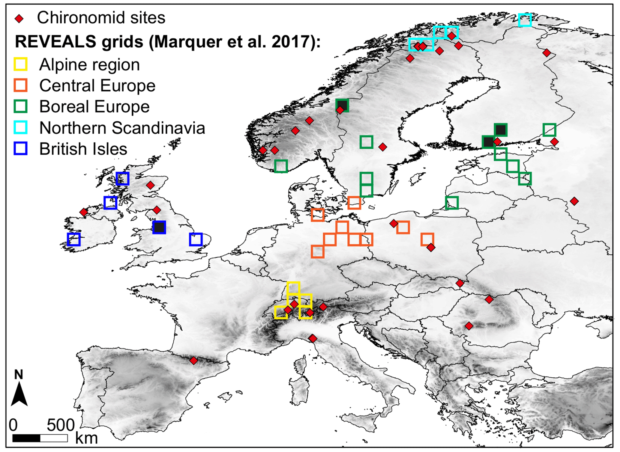
Figure 2Grid cells with REVEALS estimates of plant abundances, grouped into five biogeographical regions (for a detailed definition see Marquer et al., 2017; see figure legend for the names of the regions) and sites with chironomid data (red diamonds). Note that the four REVEALS grid cells that are colour-filled include only two small sites or one large bog (with few additional small sites) and are thus less reliable (see Sect. 2.3.2 for an explanation).
Table 2Assignment of the plant taxa used in the pollen-based REVEALS reconstructions to the plant functional types (PFTs) in the dynamic global vegetation models LPJ-GUESS and JSBACH.
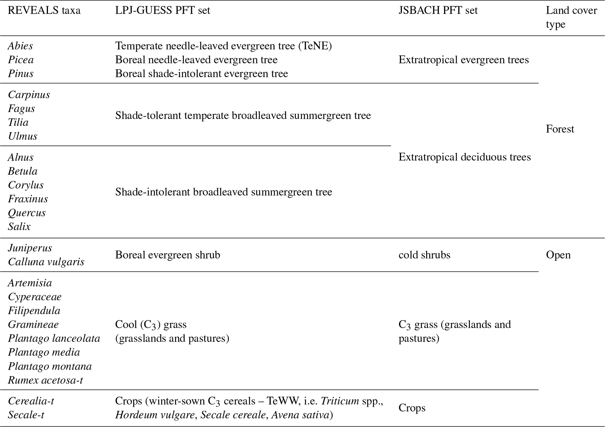
PFTs were defined following Wolf et al. (2008). However, modifications had to be made as pollen-based plant cover provides the total cover of each plant taxon irrespective of whether it belongs to one PFT or several PFTs. Therefore, each plant taxon can be included in only one PFT (Table 2). The method used to calculate mean SEs for grid cells and the PFTs is described in Li et al. (2020).
2.4 Methods used to compare DGVM-simulated and REVEALS-estimated tree cover
The differences between REVEALS and JSBACH estimates, REVEALS and LPJ-GUESS estimates, and JSBACH and LPJ-GUESS estimates have been assessed for tree cover, deciduous tree cover, and conifer tree cover in each grid cell. We calculated the absolute value of the differences between two estimates for each grid cell, and we defined a scale of agreement based on this absolute value and the data distribution over the entire study region (i.e. absolute values for all grid cells) for each time window. The first quartile and the median have been calculated. Good agreement corresponds to an absolute value of the differences between two estimates lower than the first quartile. Agreement corresponds to an absolute value of the differences between two estimates situated between the first quartile and the median. Disagreement corresponds to an absolute value of the differences higher than the median. The results have been plotted using ArcGIS 10.6 to observe the spatial distribution of the differences between the different past vegetation reconstructions.
The squared chord distance (Prentice, 1980) was calculated for each time window to evaluate the spatial dissimilarities over time between REVEALS, JSBACH, and LPJ-GUESS in terms of total, deciduous, and evergreen tree cover. The squared chord distance is commonly used to calculate the dissimilarities between two sets of data that represent assemblages, i.e. plant composition. In this study we apply it to the ensemble of grid cells across our study region; i.e. we are studying how dissimilar the spatial grid compositions between REVEALS and the DGVMs are for each time window.
We compare the vegetation change simulated by the two models JSBACH (coupled in MPI-ESM1.2) and LPJ-GUESS (forced with MPI-ESM1.2 climate) with pollen-based REVEALS reconstructions. Please note that land cover changes (decreases or increases) are expressed in absolute fractions of the grid cells; e.g. an increase in cover by 20 % at x ka from a cover of 50 % of the grid cell at y ka implies that the cover at x ka is 70 % of the grid cell.
3.1 European tree cover change since 8 ka
The two models simulate a similar European potential natural vegetation history but with very different total tree cover fractions over time (Fig. 3). LPJ-GUESS shows dense tree coverage between 80 %–100 % in large parts of Europe during the mid-Holocene and late Holocene. More open landscapes are simulated for the Mediterranean area (particularly southwestern Spain and southern Italy) and the mountainous regions of Scandinavia and the Alps. Vegetation is nearly constant until the prescribed land use forcing sets in, substantially reducing the tree cover in western, central, and eastern Europe at the 1 ka and PI time slices.
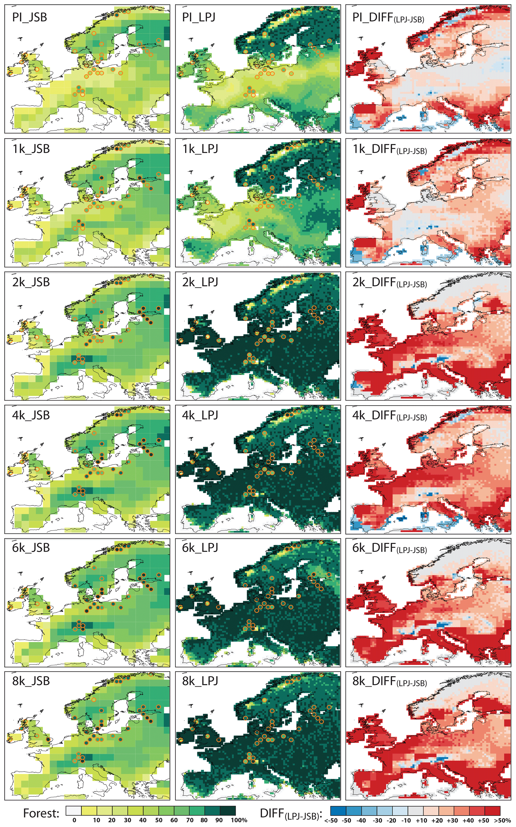
Figure 3Total tree cover fraction (in absolute fraction of the grid cells) for six time slices simulated by JSBACH (JSB) (left panels) and by LPJ-GUESS (LPJ) (centre panels) as well as the model difference (right panels). The pollen-based REVEALS tree cover (dots) is superimposed on the maps with the same colour scheme as the model results.
JSBACH generally simulates a spatial gradient similar to LPJ-GUESS, with fewer trees in the Mediterranean region and the Scandinavian mountains and the largest tree cover in central Europe. However, tree coverage is much lower in most parts of Europe during the mid-Holocene and late Holocene than simulated by LPJ-GUESS, mostly reaching tree cover fractions of 40 %–70 %. Particularly obvious are the very low tree cover fractions in the coastal areas of the Atlantic Ocean and Mediterranean Sea as well as in southern Europe, leading to remarkable differences between JSBACH and LPJ-GUESS during the mid-Holocene to late Holocene. In contrast, JSBACH simulates a slightly higher tree cover fraction than LPJ-GUESS in parts of northern Scandinavia and the Alpine region.
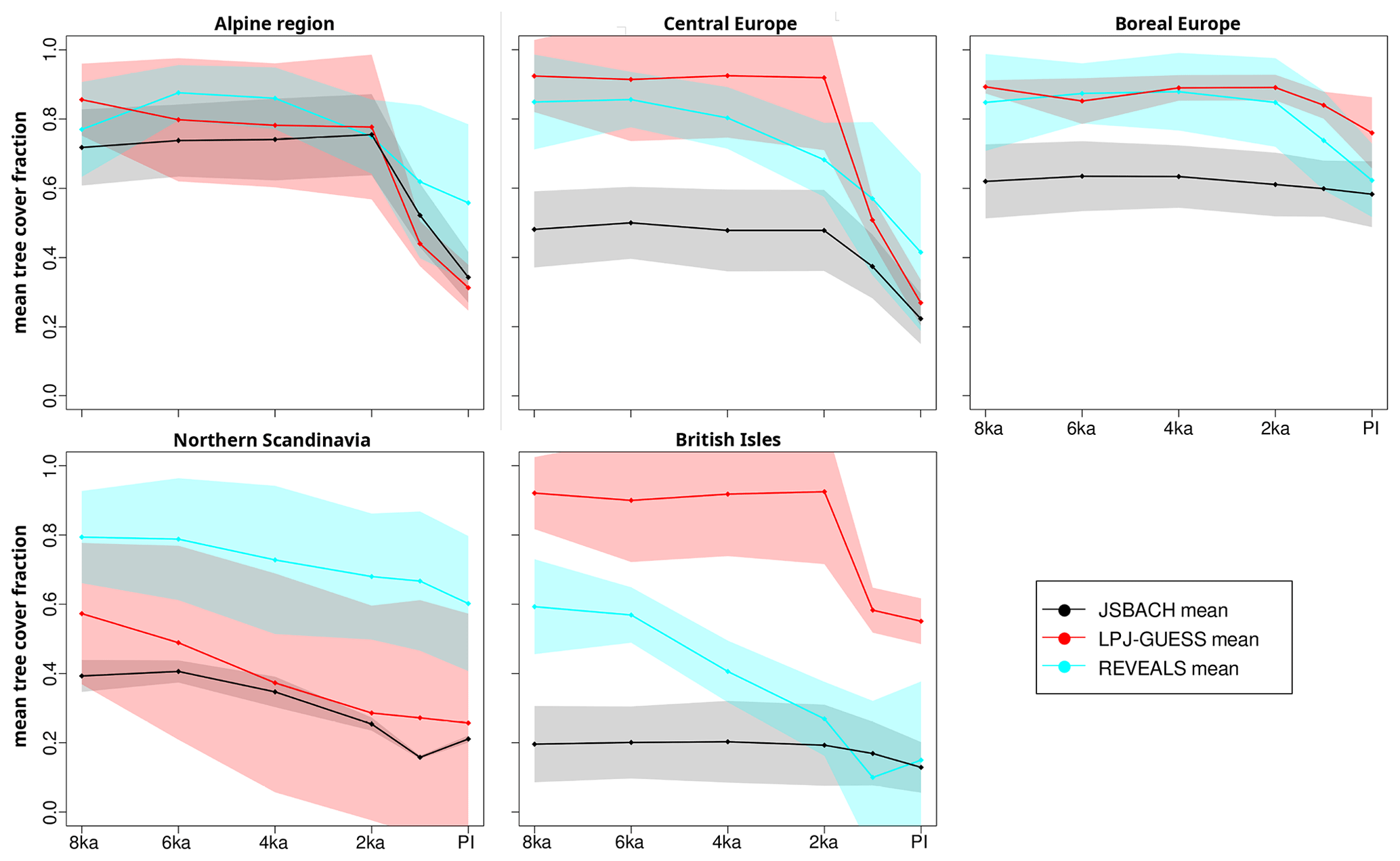
Figure 4Model-simulated and pollen-based REVEALS mean tree cover fraction averaged over the five regions as displayed in Fig. 2: JSBACH (black), LPJ-GUESS (red), and REVEALS (cyan). The inter-grid-cell ± SD (standard deviation) is shown with shading. Note that the standard errors in the REVEALS estimates are not considered. Time series are plotted based on six time slices (dots) and linearly interpolated.
As in LPJ-GUESS, JSBACH indicates relatively constant tree cover distributions until the prescribed land use is applied. Due to the higher potential natural tree cover fractions in western, central, and eastern Europe, the land use has a stronger effect in LPJ-GUESS than in JSBACH, reducing the differences between the models with respect to the total tree cover fraction for the time slices influenced by land use (1 ka and PI).
The REVEALS-based estimates of European tree coverage for 8 ka (Fig. 3) indicate dense forests in most regions, with the highest tree cover fractions along the Baltic Sea (central and boreal Europe) and in the Alpine region and a more open landscape on the British Isles. The reconstructed tree cover in northern Scandinavia is also quite high and therefore strongly deviates from the model results.
Figure 4 displays the mean trend in the different subregions simulated by the models and REVEALS based on the different time slice experiments. Since the models do not reveal much variability in the tree cover, the few simulated data points were linearly interpolated. The presented time series therefore only shows the long-term trend but cannot reflect the centennial variability.
For the Alpine region, the dynamic vegetation models and the REVEALS-based reconstructions compare well with total tree cover estimates around 70 %–85 % in the mean. REVEALS indicates a tree cover maximum at 6 ka and a decreasing trend already starting at 4 ka from about 86 % at 4 ka to approximately 56 % at PI. In contrast, the models simulate relatively constant tree coverage for the period 8 to 2 ka followed by a sharp drop in the tree cover fraction after 2 ka as a response to the prescribed land use. Tree cover is considerably reduced in all datasets and nearly halved between 2 ka and PI (from about 75 % to 35 %) in the models. The several-millennia-long mismatch in timing and intensity between the models and the reconstructions indicates not only a later onset of but also overly extensive deforestation in the models compared to REVEALS estimates.
For central Europe, LPJ-GUESS simulates constant high tree coverage of more than 90 % between 8 and 2 ka, as well as a sharp reduction (to 27 % at PI) thereafter. JSBACH reveals a similar, albeit weaker, vegetation dynamic with mid-Holocene tree cover fractions of approximately 50 % and substantially decreased tree cover at PI (∼22 %). Also, for this region, the REVEALS-based reconstructions show a different temporal trend. The decrease in tree cover begins as early as 6 ka and accelerates towards PI. At 8 ka, tree cover is estimated at 85 %, agreeing well with the LPJ-GUESS estimates. Tree cover is nearly halved to 41 % at PI according to REVEALS. The reduction in tree coverage after 2 ka parallels the trend in the JSBACH simulation, but with higher tree cover fractions.
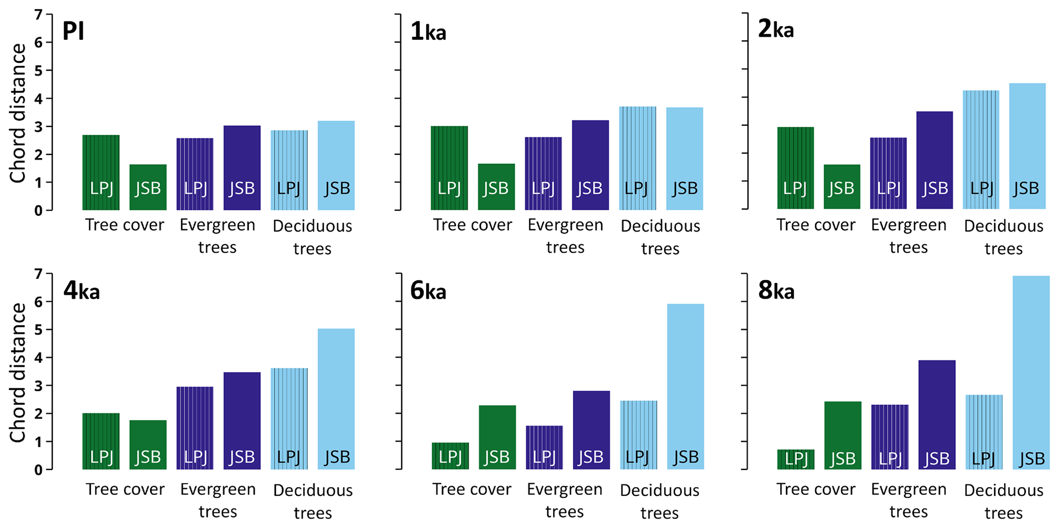
Figure 5Chord distance between JSBACH and REVEALS (no pattern) and between LPJ-GUESS and REVEALS (vertical stripes) for total tree cover (brownish), evergreen trees (dark green), and deciduous trees (light green) for six time slices.
LPJ-GUESS and REVEALS indicate similarly high (∼85 %–90 %) mid-Holocene tree cover fractions in boreal Europe, whereas JSBACH simulates much fewer trees (∼60 %). Both REVEALS and LPJ-GUESS show relatively constant tree cover between 8 and 4 ka. In REVEALS, the tree cover fraction decreases slightly from 4 ka but is substantially reduced (by 36 %) only in the last ∼2000 years. In LPJ-GUESS, tree coverage declines by only 15 % between 2 ka and PI. It is difficult to figure out the effect of land use in this model setup, but the differences in the magnitude of the tree cover decrease could indicate an underestimation of the prescribed land use intensity in this region in the models. In JSBACH, land use has hardly any effect at all in the regional mean.
For northern Scandinavia, the models and the REVEALS reconstructions show a similar trend of steadily decreasing tree cover during the Holocene but differ significantly in absolute tree cover. REVEALS estimates tree coverage of approximately 80 % at 8 ka, declining to 60 % at PI. LPJ-GUESS simulates a mean tree cover of 58 % at 8 ka and 26 % at PI. In JSBACH, the simulated tree cover fraction is reduced from 40 % at 8 ka to 21 % at PI. The relative decrease in tree coverage (tree cover is halved in both models) is thus much stronger in the models than estimated by the REVEALS-based reconstructions.
The models and reconstructions show the largest deviations on the British Isles. While JSBACH indicates very low tree cover fractions of approximately 20 % at 8 ka and a slight decrease in tree cover after 2 ka to 13 % at PI, LPJ-GUESS simulates high tree cover fractions during the mid-Holocene (∼92 %) and a sharp drop to 58 % between 2 and 1 ka. REVEALS estimates a tree cover of 60 % at 8 ka and a constant decrease between 6 and 2 ka to 27 %, followed by a stronger drop in tree cover towards 1 ka (to 10 %) and a slight recovery towards PI (to 14 %).
In summary, the inter-model spread is largest in the British Isles and central Europe as well as in southern Europe (no REVEALS region) with much lower tree cover fractions in JSBACH than simulated by LPJ-GUESS. Compared to the REVEALS estimates, JSBACH underestimates the tree cover in practically all regions and during most of the time slices except for the Alpine region, whereas the LPJ-GUESS-estimated tree cover is comparable to the REVEALS estimates in boreal and central Europe. However, LPJ-GUESS significantly underestimates the tree cover in northern Scandinavia and overestimates it in the British Isles. The models suggest rather constant European tree coverage between 8 and 2 ka, whereas the REVEALS-based reconstructions show a stronger dynamic with the tendency of a mid-Holocene (6 ka) maximum tree cover followed by a steady decline. The prescribed land use has a larger effect in LPJ-GUESS than in JSBACH, indicating differences in its implementation and a higher tree cover level at the onset of land use in LPJ-GUESS. Compared to the REVEALS reconstructions, the prescribed land use in the models appears to be too large in parts of central and western Europe (particularly in the Alpine region) and too small in boreal Europe.
3.2 REVEALS versus vegetation models
3.2.1 Temporal distribution of the differences
The calculated chord distances between the datasets indicate that the simulated tree cover pattern in LPJ-GUESS is overall in better agreement with REVEALS during the mid-Holocene than the one inferred by JSBACH (Fig. 5). Particularly for the 8 ka time slice, the total tree cover simulated by LPJ-GUESS compares very well with the reconstructions, yielding a chord distance below 1. The chord distance for the evergreen and deciduous tree cover is substantially higher, indicating that the ratio of deciduous to evergreen forest is not quite as well-represented by LPJ-GUESS.
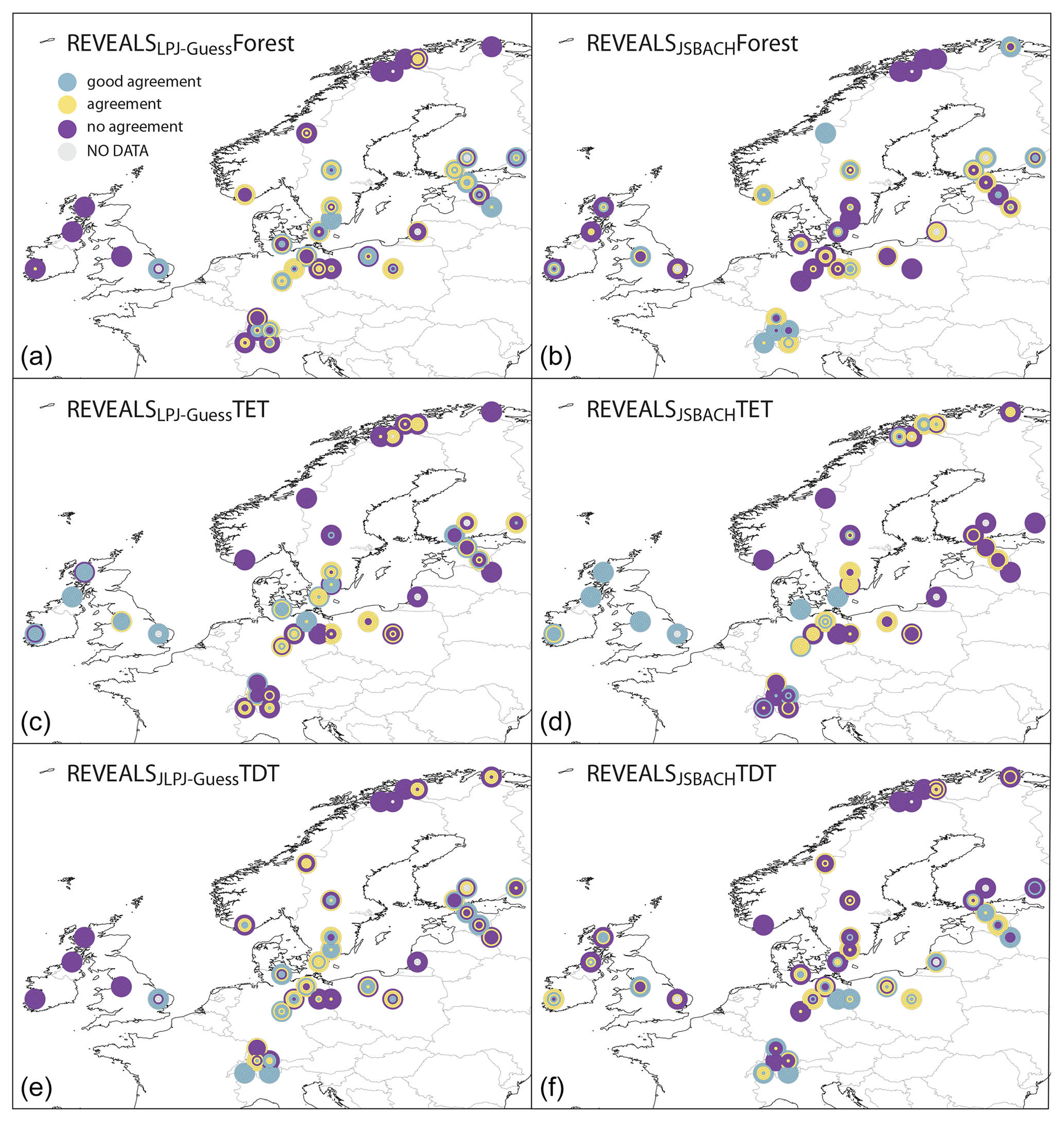
Figure 6Agreement between REVEALS and LPJ-GUESS (a, c, e) and between REVEALS and JSBACH (b, d, f) for total tree cover (forest, a, b), evergreen trees (TET, c, d), and deciduous trees (TDT, e, f) (see legend for colours). The plot is based on a three-scale agreement index to quantify and evaluate the spatial differences between the model-simulated vegetation and the pollen-based REVEALS plant cover in each of the REVEALS grid cells (see Sect. 2 for details). The six circles display the results for the six time slices, from the oldest (8 ka, outermost circle) to the younger one (PI, innermost circle).
The results for JSBACH suffer from the severe underestimation of deciduous trees compared to REVEALS. This is reflected in the very high chord distance at 8 ka. However, the spatial distribution of evergreen trees is better represented by JSBACH at 8 ka. The agreement of the two different models with REVEALS converges towards 1 ka and PI. The representation of the deciduous trees gets continuously better in JSBACH, while it gets worse in LPJ from 6 to 2 ka. This affects the model–data agreement with respect to the total tree cover. The mismatch in tree cover between LPJ-GUESS and REVEALS increases towards 1 ka. For JSBACH, the chord distance to the REVEALS-estimated tree cover distribution is relatively constant until 4 ka and gets better afterwards.
Since the mismatch to the reconstructions in the distribution of evergreen trees is relatively constant in both models, the improvement of the agreement in total tree cover between the DGVMs and REVEALS is clearly driven by the increasingly better representation of deciduous trees in the DGVMs with time, even if the cover fractions of the evergreen trees in both models generally agree better with the REVEALS estimates than the deciduous tree cover fractions. Since 4 ka, the total tree cover distribution simulated by JSBACH agrees better with REVEALS than the LPJ-GUESS-simulated distribution, but the misrepresentation of the ratio of evergreen to deciduous trees remains.
Overall LPJ-GUESS shows the best agreement with REVEALS for the 6 ka time slice, followed by the PI time slice. JSBACH also indicates an improvement of the agreement with respect to the cover fraction of evergreen trees for 6 ka. However, it agrees best with REVEALS for PI conditions.
3.2.2 Spatial distribution of the differences
We calculate a three-scale agreement index to quantify and evaluate the spatial difference between the models and the REVEALS-based reconstructions in each grid cell (see the Methods section). The pattern indicates model-specific regions with systematic agreement or disagreement (Fig. 6). For instance, JSBACH fails to reproduce the REVEALS mid-Holocene tree cover fraction in large parts of central Europe, the Baltic States, and southern Sweden, while LPJ-GUESS shows reasonably good overall agreement in these regions. Both models produce tree cover estimates not comparable with REVEALS reconstructions for the British Isles. For JSBACH this mismatch gets slightly better towards PI, mainly due to an improved representation in some grid cells in northern Germany, Scotland, and Ireland. In most grid cells on the British Isles and in western Germany, the fractional coverage of evergreen trees simulated by both models has better agreement with the REVEALS estimates than the deciduous tree cover fraction, underlining the previous finding of the deciduous trees as a driver of the model–data mismatch. However, in eastern Europe (Poland, Baltic States) the deciduous tree coverage simulated by both models is more in line with the REVEALS estimates than the evergreen tree coverage.
The tree cover fraction in the Alpine region simulated by JSBACH corresponds better to the REVEALS estimates than in other regions until the land use in the model sets in. All grid cells in these regions receive agreement or even good agreement with respect to the JSBACH-derived total tree cover. In contrast, LPJ-GUESS indicates only some agreement in the central Alpine region. The fraction of deciduous trees is mostly in agreement for both models during the mid-Holocene, but the agreement decreases towards the late Holocene. The simulated fractions of evergreen trees disagree with the REVEALS-based estimates at all time slices.
In most grid cells of northern Scandinavia, the deciduous and total tree cover do not match the reconstructions during all time slices. The evergreen trees, however, show agreement in many grid cells, which becomes even better towards 1 ka.
The total tree coverage in REVEALS and JSBACH compares well in the domain of southern–central Norway to central Sweden and southern Finland, reaching values of agreement to good agreement in most grid cells during all periods. LPJ-GUESS does not agree as well as JSBACH with REVEALS, particularly in southern Norway. Interestingly, in these regions JSBACH is not able to capture the REVEALS-estimated fractions of evergreen and deciduous trees, indicating a misrepresentation of the ratio of the different tree types. In contrast, LPJ-GUESS captures the REVEALS deciduous tree cover fraction for the late Holocene.
Based on the results presented in Figs. 5 and 6, it is not possible to determine which model is overall more consistent with REVEALS. The agreement strongly depends on the region. It should be noted, however, that in a statistical sense the thresholds for the three-scale agreement indices are equal for both models, but the absolute values of the thresholds may differ, depending on the general spatial variability in the models that is higher in JSBACH than LPJ-GUESS. This statistical definition of the threshold allows JSBACH to still be rated in the category “agreement” with larger absolute differences to REVEALS.
Comparison of the tree cover fractions and their spatial and temporal distributions as simulated by the DGVMs and estimated from pollen data by the REVEALS model is challenging. When compared with REVEALS, JSBACH rather underestimates European tree cover during the mid-Holocene and late Holocene, while LPJ-GUESS mainly overestimates the tree coverage, at least in those time slices without human impact prescribed to the models (8 to 2 ka). In addition, the model agreement with the REVEALS results shows a spatially varying pattern that is different for each model. Whereas JSBACH reveals the strongest mismatch to the reconstructions in central Europe during all periods, LPJ-GUESS shows relatively good agreement in this region. Both models fail to reproduce the tree cover history on the British Isles and in northern Scandinavia. For the Alpine region, the JSBACH-simulated tree cover fractions correspond well to the REVEALS estimates, while the LPJ-GUESS values more often disagree.
In most regions, the models are not able to simulate the correct ratio of deciduous to evergreen trees, but the evergreen tree cover distribution is generally more in line with the REVEALS data than the deciduous tree coverage. While LPJ-GUESS shows relatively good overall agreement with REVEALS at 8 ka and particularly at 6 ka, the mismatch increases from 4 to 1 ka. In contrast, the distributions simulated by JSBACH continuously improve (in the mean) towards PI, indicating a convergence of the model results through time.
We assume the following possible reasons behind the model–data differences and discuss them thoroughly in the next sections (here, “model” refers to the two DGVMs and “data” to the pollen-based REVEALS plant cover):
- a.
climate and spatial resolution biases in the models;
- b.
oversimplified vegetation dynamics in the models;
- c.
modern parameterizations and tuning of the models to modern conditions;
- d.
differences between the pollen-based REVEALS estimate of deforestation due to land use and the prescribed land use as well as differences in the land use implementations in the models;
- e.
shortcomings of the data, i.e. caveats of the REVEALS model itself and the pollen-based reconstructions of plant cover used in this study.
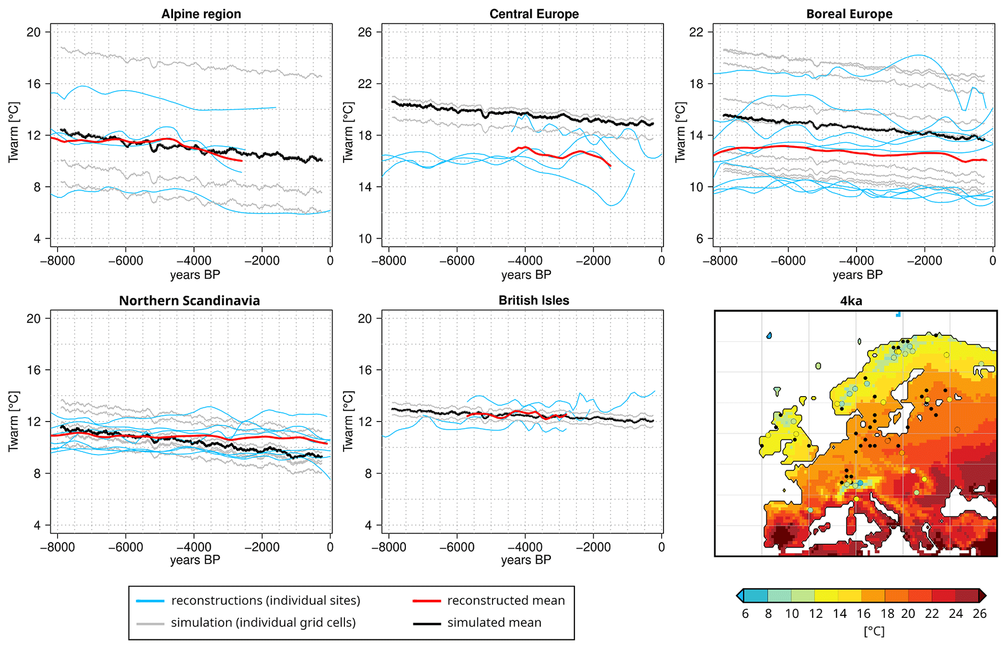
Figure 7Comparison of the temperature of the warmest month (Twarm) (∘C) prescribed to LPJ-GUESS and chironomid-based temperature reconstructions for the study regions (Fig. 2). Please note that the LPJ-GUESS forcing data are based on the climate simulated by MPI-ESM1.2 that has been added as an anomaly (from PI) to the CRU TS4.0 dataset (Harris et al., 2020). Here the model data have been smoothed by a 200-year running mean, and the reconstructions has been smoothed and interpolated on an equally distant time axis. See Table B1 for further details on the reconstructions. For each region, we have plotted the simulated Twarm in the individual grid cells with chironomid-inferred Twarm available (grey) and their mean (black), as well as the individual chironomid-inferred Twarm (blue) and their mean (red). In the bottom right panel, we show the model-simulated (gridded) and chironomid-inferred (colour dots) Twarm (∘C) at 4 ka. The black dots represent the location of the grid cells with pollen-based REVEALS plant cover reconstructions.
4.1 Effect of biases in the simulated climate and climate input fields on the tree cover distribution
Based on a previous study (Dallmeyer et al., 2021) analysing a slightly different Holocene MPI-ESM1.2 simulation, we assume summer temperature to be the main climatic driver of the simulated vegetation in the European regions considered here. To infer possible biases in the simulated climate trend, we compare the LPJ-GUESS temperature forcing data with chironomid-based reconstructions of the temperature of the warmest month (Twarm) (Fig. 7), extracted from the synthesis of Kaufman et al. (2020a, b) and a few other sources (references are given in Table B1). It should be stressed, however, that temperature reconstructions based on chironomids may be subject to various caveats, whose detailed description is beyond the scope of this paper. Other environmental changes, in e.g. nutrients, anoxia, and salinity, can indeed also lead to changes in chironomid assemblages, which may affect the chironomid-inferred temperatures (e.g. Velle et al., 2010). Nevertheless, the distribution of chironomid assemblages generally strongly correlates with the warm-season air and lake temperature in the temperate and subarctic regions, although the causal relationships are still not fully understood (e.g. Eggermont and Heiri, 2012).
The model-based mean temperature dynamics are well in line with the reconstructions. Simulated Twarm levels in the Alpine region are different for all sites and cover a wider range than the reconstructions indicate. While Twarm decreases relatively uniformly at all sites after 8 ka in the model, two of the four reconstructions show a climatic optimum between 7 and 4 ka. This is consistent with the maximum tree cover fraction in the REVEALS data at the 6 and 4 ka time slices in this region. The good agreement of the simulated and reconstructed mean temperature of the warmest month reflects the similarly high tree cover fractions estimated by REVEALS and simulated by both models.
For central Europe, only one chironomid-based reconstruction exists in Kaufman et al. (2020a), i.e. for Lake Zabieniec (Płóciennik et al., 2011). For this record, new reconstructions have been published recently (Luoto et al., 2019; Kotrys et al., 2020). With a mean Twarm of around 16 ∘C, these reconstructions indicate a substantially, roughly 5 ∘C, cooler summer climate than prescribed to LPJ-GUESS at 8 ka. Furthermore, the reconstructions reveal stable or slightly increasing Twarm for the mid-Holocene in contrast to the decreasing trend in the model. For the late Holocene, the reconstructions of the Zabieniec record diverge strongly, revealing contradictory changes in Twarm, but all indicate a much colder climate in this region than revealed by the simulated climate used to force LPJ-GUESS. However, a chironomid-based reconstruction from northern Poland (Lake Spore, Pleskot et al., 2022) is well in line with the model. Both show declining Twarm from about 19 to 17.5 ∘C during the late Holocene and only reveal substantial differences for the last 500 years. The difference in Twarm level at Lake Zabieniec may act as an indicator of a model-derived climate that is slightly too warm in the southern part of central Europe. This warm bias may also extend to the southeastern part of the simulation region, displayed exemplarily for the 4 ka time slice (Fig. 7). This warm bias may contribute to the slightly overestimated tree cover fraction in LPJ-GUESS compared to the REVEALS estimates in central Europe.
In boreal Europe, model-based Twarm is higher by approximately 2–3 ∘C during the entire period compared to the chironomid-based reconstructions. While the model indicates an almost linear decrease in Twarm since 8 ka, some reconstructions reveal a warming towards 6 ka and decreasing temperatures afterwards. This dynamic is also visible in the mean over the region and nicely fits the REVEALS-based reconstruction of tree cover change. Regardless of these discrepancies, the modelled temperature range is still located well within the tolerance limits of boreal tree taxa. Since the tree cover fractions are similar in LPJ-GUESS and REVEALS, this bias in temperature does not affect the total tree cover distribution.
Simulated temperatures of the warmest month are on a level similar to the reconstructions in northern Scandinavia during the mid-Holocene, not explaining the 20 % lower tree cover fraction in LPJ-GUESS compared to the REVEALS estimates. The reconstructions reveal only a slight decrease in Twarm since 8 ka, in contrast to the stronger decrease in the model. These differences in temperature trend are in line with the slight deviations in the rate of tree cover decline between LPJ-GUESS and REVEALS in northern Scandinavia. However, both modelled and reconstructed Twarm averages fluctuate close to the 10 ∘C, with the modelled temperature falling below it during the late Holocene. The 10 ∘C limit is – according to the known Köppen rule (Köppen, 1936) – accepted as a delimiter of boreal forest distribution, and Twarm falling under this limit could be a possible cause for low model-based tree cover estimates.
Tree cover fractions simulated by LPJ-GUESS show the highest discrepancy with the REVEALS estimates on the British Isles, overestimating tree coverage by more than 30 %. While the mean trend in Twarm during the period 6 to 3 ka is relatively similar (slightly decreasing) between the prescribed climate and the chironomid-based reconstructions, LPJ-GUESS shows a constant, large tree cover until land use sets in and REVEALS indicates a strong decrease in tree cover starting at 6 ka. These deviations in total tree cover changes through time cannot be explained by the simulated summer temperature.
Comparing the chironomid-based reconstructions with the climate simulated by MPI-ESM1.2 directly is not very meaningful, since many of the chironomid sites are located in mountainous regions. Due to the coarse spatial resolution of the model, one can expect the climate to be rather too warm and to show much stronger differences in annual extremes than in the mean over the seasons. The evaluation of the pre-industrial climate (Appendix A and Fig. A1) reveals only minor differences in the seasonal temperature mean between the CRU TS4.0 data and the simulated MPI-ESM1.2 climate for PI.
The total tree coverage simulated by JSBACH agrees well with the LPJ-GUESS results in the Alpine region and northern Scandinavia with Twarm-limited tree growth. JSBACH strongly underestimates tree coverage in central Europe and for the British Isles. The former region does not experience any substantial differences in seasonal temperature, and the wetter climate in MPI-ESM1.2 probably does not induce changes in total tree coverage as the land cover of the region is not moisture-limited. The latter region is affected by strong deviations in the precipitation pattern with a much drier and rather warmer climate at most grid cells for which REVEALS reconstructions are available. Since the strong differences in tree coverage compared to LPJ-GUESS cover the entire British Isles, and thus also the regions with overestimated precipitation, these climate biases cannot be responsible for the strong deviations in vegetation composition between the models.
In boreal Europe, winter and summer climate in MPI-ESM1.2 is slightly cooler than observed. Since the climate is nevertheless well within the climatic tolerance range for extratropical tree PFTs in JSBACH, this does not limit the establishment of trees in JSBACH. However, while JSBACH has only one deciduous and one evergreen PFT for temperate and boreal conditions, the PFT list of LPJ-GUESS includes several PFTs developed specifically considering boreal conditions (Table 2). This may contribute to the substantially lower tree coverage in JSBACH compared to LPJ-GUESS.
We conclude that climate (temperature) biases are not the main driver of differences in the total tree cover fraction between the REVEALS estimates and the vegetation models and between LPJ-GUESS and JSBACH in most of the regions. The simulated climate trends are mostly in line with the chironomid-based reconstructions, and in the case of differences, these cannot cause the discrepancies in the tree cover trend. Therefore, it is highly likely that land use is the reason for the much earlier tree cover decline in the reconstructions than in the models and that land use is the main driver of the long-term Holocene tree cover change in Europe.
4.2 Effect of oversimplified vegetation and soil dynamics in the models
Even though we have adjusted the PFT distributions calculated with the different methods to be more compatible with each other, various technical factors can lead to differences between the DGVMs and between these and REVEALS. Many processes can only be represented in a simplified form or have not been implemented in vegetation models yet. For instance, vegetation is only aggregated in a few PFTs, which do not match each other or REVEALS in number or definition (Table 2), and not all PFTs considered in REVEALS have a counterpart in the models. Whereas REVEALS reconstructions reflect actual land cover including understorey vegetation, wetlands, and other specialized communities, the models estimate terrestrial high-ground vegetation only. In contrast, the models calculate a fraction of uncovered soils that cannot be determined in pollen-based reconstructions and is therefore not included in the REVEALS data. LPJ-GUESS considers early and late successional deciduous and evergreen tree types separately, whereas JSBACH distinguishes only one deciduous and evergreen tree type. This differentiation allows for quick re-establishment of the tree cover after disturbance or climate-induced mortality, making LPJ-GUESS-simulated forest cover considerably more stable and less affected by random deforestation events.
Seed dispersal is not included in either of the models. Seeds are assumed to be available everywhere all of the time, whereas in the real world they need to be transported before a tree can grow in a new spot under favourable environmental and site conditions for tree growth. Moreover, depending on existing vegetation and tree species, the success of the establishment of a tree species and thus their regional abundance might differ. Although the dispersal- and migration-related delays in the establishment can mostly be expected in connection with the reforestation of Europe during the post-glacial and early Holocene period (Giesecke et al., 2017), they could be the reasons for the differences in the mid-Holocene tree cover changes between the models and REVEALS. The models show rather stable, in some regions slightly decreasing, mean tree cover with time, while REVEALS estimates tree cover maxima between 6 and 4 ka for grid cells in boreal and central Europe as well as in the Alpine regions.
In addition, the models have simplified soil dynamics and do not consider changes in soil type or soil build-up. Permafrost soils, peatland or wetlands, and blanket bogs are not represented in these simulations. Therefore, the models lack representation of important habitats such as mires and bogs, whose (mainly treeless) vegetation increases the openness in reconstructed vegetation. Most of Europe had substantially more wetlands in the past than at present with its highly drained landscapes (Čížková et al., 2013). Furthermore, several European countries have ca. 15 (Sweden, Ireland and Scotland) to 30 % (Finland) of territory occupied by blanket bogs and wetlands even today. Fyfe et al. (2013) highlight the considerable bias in landscape openness between the British Isles and continental Europe throughout the Holocene in the REVEALS-based study and suggest that this could at least partly be due to the considerably higher proportion of wetlands and uplands in the land cover of the British Isles compared to continental Europe. The formation of blanket bogs, typical for cool and hyper-oceanic climates, was accelerated by climate cooling starting ca. 6 ka (Gallego-Sala et al., 2016), which may, together with anthropogenic deforestation, explain the small woodland cover. As a result of the disregard for wetlands, models tend to overestimate the tree cover fraction in wetland-rich regions. This potential overestimation may explain the deviations between REVEALS and LPJ-GUESS, revealing much higher tree cover fractions in the British Isles and slightly higher tree cover in boreal and central Europe than REVEALS.
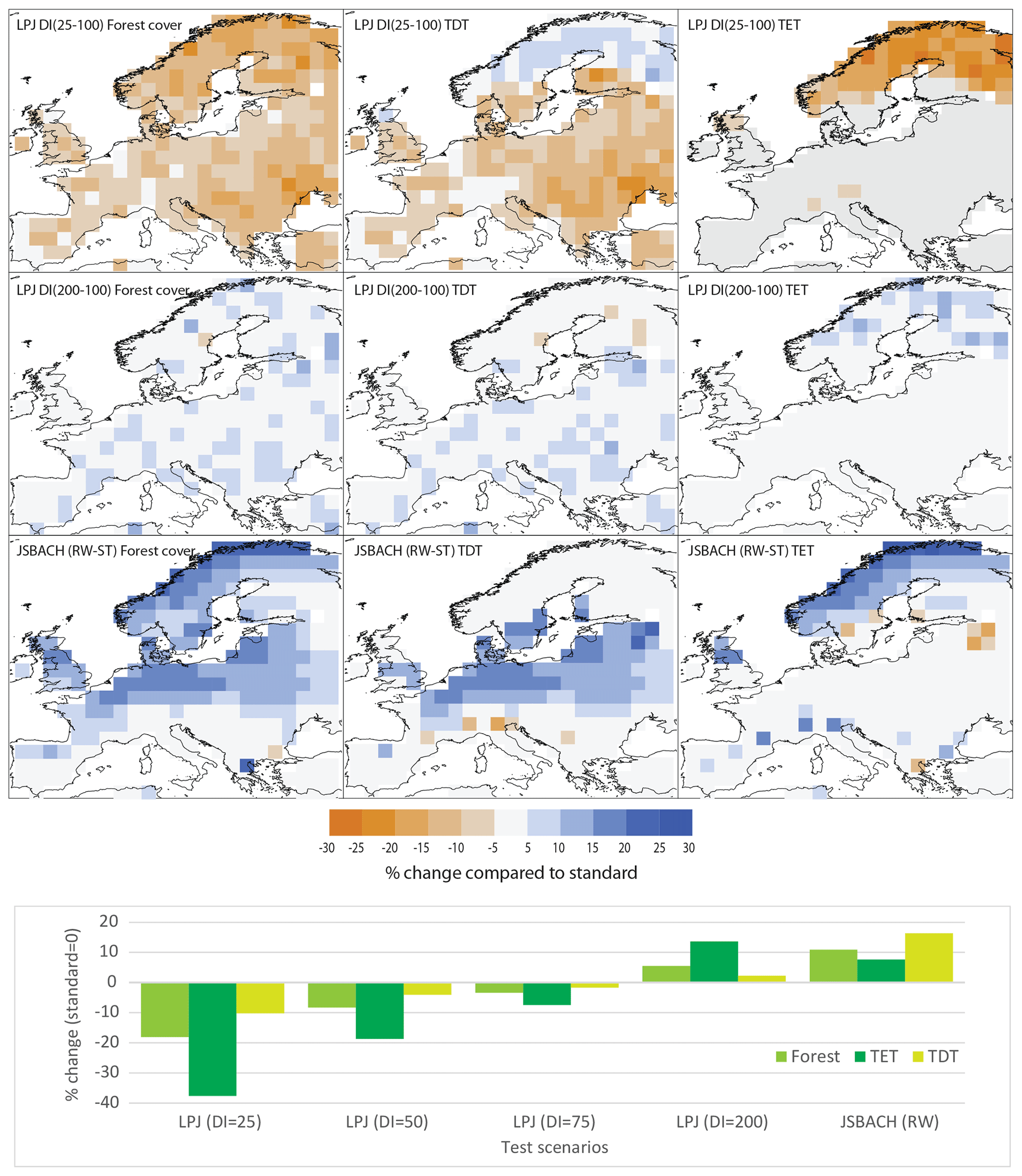
Figure 8Sensitivity test with different disturbance settings. Upper nine panels: tree cover difference (in absolute % of the grid cell area) between LPJ-GUESS simulations with an occurrence interval of 100 years (standard setup) and 25 years (upper row panels) or 200 years (second row panels) and between the JSBACH simulations in the standard setup (ST, used in this study) and with a halved wind damage scaling parameter (RW) (bottom row panels). For each setup, the differences in cover of total trees (forest) (left column panels), deciduous trees (TDT) (middle column), and evergreen trees (TET) (right column panels) are shown. For LPJ-GUESS, occurrence intervals of e.g. 25 years mean that stochastic patch-destroying disturbance occurs once per 25 simulation years. Lower panel (bar plot): difference in simulated tree cover fractions between the simulations with the standard setup and the four different disturbance occurrence intervals (DI) in LPJ-GUESS (LPJ) and between the standard and reduced wind throw (RW) simulations in JSBACH, averaged over the entire region.
4.3 Effect of modern parameterizations and of tuning of the model to modern conditions
Each vegetation model uses a different way of representing vegetation or incorporating processes such as PFT establishment, plant competition, natural mortality, or reductions of plants by disturbances such as fire, wind throw, and insects. However, they share the implemented equations of these processes, and the thresholds used (e.g. for the bioclimatic tolerance) are validated and calibrated using modern observations. Parameters are tuned to meet modern vegetation distributions and do not change in time. This means that all basic settings such as bioclimatic limits, allocation and mortality timescales, or sensitivity to disturbances are assumed to be constant over the simulation time. While it is true that species-specific bioclimatic limits change slowly and most of the simulations do not reach the timescales necessary for considerable changes, the validity of the assumption that present-day plant distribution is in equilibrium with climate is questionable. Modern species distribution patterns are heavily influenced by centuries of agriculture and forest management. The recent abrupt global climate change combined with other human impacts on plant species has enhanced the difference between potential and realized niches, making it highly doubtful that the current species distribution limits would represent the actual bioclimatic envelope of plant species in Europe. Furthermore, these values may not be valid for climate states totally different from today, such as the mid-Holocene; this also refers to the concept of no-analogue communities (e.g. Williams and Jackson, 2007). The simulated tree cover in areas occupied by forest biomes is largely dependent on the implemented disturbance extent, severity, and interval. However, the causes and consequences of disturbances are largely different in natural and human-influenced landscapes. The mid-Holocene natural forests were probably much more stable and less sensitive to disturbances than present-day forests that are heavily altered by human interventions.
We hypothesize that the large underestimation of the tree fraction on the British Isles and in central Europe in JSBACH compared to REVEALS is a consequence of too much wind throw in the model. In contrast, the overestimated tree cover fraction in LPJ-GUESS may at least partly be related to a spatial scale and frequency of disturbance occurrences in LPJ-GUESS that are too small. We tested this hypothesis in a sensitivity study in which we extended the MPI-ESM1.2 spin-up run (8 ka forcing) with halved sensitivity of the trees to the wind throw (i.e. halving the wind damage scaling parameter in JSBACH). For LPJ-GUESS, we performed a set of simulations changing the interval between disturbance occurrences from 25 to 50, 75, and 200 years using the 8 ka climate forcing. The standard setup used in the comparison with REVEALS and JSBACH above is 100 years.
Wind throw reduction substantially increases the tree cover simulated by JSBACH in a broad area in mid-Europe (48–58∘ N), including the regions of the British Isles and central Europe, as well as along the Norwegian Atlantic coast (Fig. 8). These are also regions in which JSBACH substantially deviates from REVEALS and strongly underestimates tree cover in the transient simulation. However, in the other regions, only a few REVEALS grid cells are affected, and thus in regional means over the grid cells, the effect of wind throw is smaller.
The disturbance frequency tests with LPJ-GUESS show that each reduction of the occurrence interval by 25 years leads to approximately 4 % less tree cover. This reduction is mostly related to a decrease in the cover of the evergreen PFTs (Fig. 8). The deciduous PFTs are not so heavily affected, as the disturbance gives some advantage to the early successional deciduous PFT (Table 2) that was parameterized keeping in mind quick establishment and growth. Therefore, the shortened disturbance interval leads to an increased representation of deciduous trees at the expense of evergreen ones in northern and eastern Europe (Fig. 8). While LPJ-GUESS-simulated total tree cover is in general already in rather good accordance with REVEALS reconstructions, especially during the mid-Holocene, the conformity could be improved by increasing the disturbance frequency.
4.4 Effect of land use
European land cover was affected by humans during most of the Holocene. Pollen-based studies show the first traces of crop cultivation in southern Europe (Eastern part of the Mediterranean basin) more than 10 000 years ago and its spread to the southern fringe of northern Europe during the following 6 millennia (Githumbi et al., 2022a). This transition to agrarian subsistence led to substantial anthropogenic deforestation of large parts of Europe. Particularly early, the coastal areas of western Europe were strongly affected and had already lost half of the natural forest cover 3500–5500 years ago (Roberts et al., 2018). While pollen-based studies can give detailed insights into land cover development in an area, these records are often not quantitative, are not spatially continuous, and do not have a high (preferably annual) resolution, all prerequisites of input datasets for vegetation models. New pollen-based reconstructions by Githumbi et al. (2022b) address most of the above-listed obstacles, providing excellent-quality, quantitative, and proxy-based continental-scale land cover reconstructions for Europe during the Holocene. However, while these reconstructions are suitable for validation of vegetation model performance and, once interpolated into spatially continuous datasets, for usage as land cover representation in climate models, these reconstructions do not distinguish between the natural and anthropogenic land cover types and therefore cannot be directly used as an anthropogenic land cover change (ALCC) input to vegetation models. There are no attempts at using land use inferred from pollen-based REVEALS reconstructions of plant cover in DGVMs published so far. Most DGVMs use prescribed land use derived from various ALCC scenarios such as KK10 (Kaplan et al., 2009) and HYDE 3.2 (Klein Goldewijk et al., 2017). However, KK10, HYDE, and other ALCCs exhibit large discrepancies in their estimates of the starting time, spatial pattern and intensity of anthropogenic land cover change, making it a challenge to simulate the effect of human-induced vegetation changes with DGVMs (Kaplan et al., 2017; Gaillard et al., 2010).
Here we used a preliminary version of the LUH2 dataset by Hurtt et al. (2020) that assumes no human interference with land cover prior to 2 ka. The increased disagreement between LPJ-GUESS and REVEALS for the British Isles and some central and boreal European sites for 4 and 2 ka is probably due to considerable anthropogenic deforestation of these areas prior to 2 ka. During the last 2 millennia the overall agreement between the models (especially JSBACH) and REVEALS increases, showing the significance of accounting for anthropogenic deforestation.
In the models, substantially different approaches are used to handle land use. While in LPJ-GUESS a certain grid cell fraction is reserved for land-use-related land cover types, JSBACH calculates natural vegetation first and afterwards applies land transitions with land use types preferentially replacing grasslands. These differences in implementation of land use explain the larger impact of land use on LPJ-GUESS-simulated than JSBACH-simulated tree cover. LPJ-GUESS-simulated natural vegetation dynamics agree well with REVEALS-estimated plant cover at 8 and 6 ka, while JSBACH underestimates tree cover. The more the landscape is affected by humans, the greater the differences in tree cover between LPJ-GUESS and REVEALS, since the full scope of actual land use in the past cannot be reproduced by the models. JSBACH simulates a rather open landscape, and prescribed ALCC has – due to specifics of its implementation – relatively little impact on the tree cover fraction. The combination of these two characteristics leads to a convergence of REVEALS and JSBACH tree cover over time and space through the last 2 millennia. LPJ-GUESS, differently from JSBACH, applies the prescribed ALCC proportions directly, making the accuracy of the ALCC dataset used especially important. The increased disagreement of the models compared to REVEALS in the Alpine region suggests that anthropogenic deforestation that is too strong has been prescribed in this area.
4.5 Caveats of the REVEALS model and pollen-based reconstructions of plant cover
Many of the assumptions of the REVEALS model are violated in the “real world” and/or violated in the past, which has been described and discussed in detail (e.g. Hellman et al., 2008a; Sugita et al., 2010; Mazier et al., 2012; Trondman et al., 2015; Li et al., 2020). The effects of the violation of assumptions cannot be quantified and accounted for, i.e. REVEALS estimates cannot be corrected for these effects. Therefore, possible effects of the violation of assumptions must be considered possible causes behind discrepancies between REVEALS estimates of plant and PFT cover and DGVM-simulated PFT cover. Because topography is not accounted for in the REVEALS model and reliable reconstructions in mountainous regions require a large number of pollen records from large lakes representing the major altitudinal vegetation zones (Marquer et al., 2020), the REVEALS estimates used here need to be considered uncertain in the Scandinavian mountains and the Alps, which may explain discrepancies with DGVMs at the grid-cell-scale level in these areas (Fig. 3). At the regional scale, REVEALS, LPJ-GUESS, and JSBACH agree when standard deviations are considered (Fig. 4). REVEALS tree cover for the grid cell with four pollen records from small bogs (Britain; Fig. 2) may be biased towards local plant cover on the bogs (i.e., overestimated cover of open land) because there are no additional pollen records from large lakes (or several small lakes) in the grid cell that would “correct” the mean REVEALS estimate towards less open land. This bias could contribute to the significant discrepancy between REVEALS and the two DGVMs for this grid cell.
REVEALS reconstructs the cover of individual plant taxa rather than the cover of PFTs or land cover types (such as “open land”). When the REVEALS taxon-based estimates are summed into PFTs or land cover types, the cover of individual plant taxa cannot be distributed between several PFTs or land cover types. This shortcoming should not affect the comparison with the PFT cover simulated by both DGVMs in this study given that the simulated woody PFTs include only woody plants and open land only herbs. Furthermore, acceleration of the development of Calluna heathland at the expense of woodland from 6 ka in coastal areas of westernmost Europe is due to land use (grazing and burning) (Nielsen et al., 2012) and could explain some discrepancies in the cover of open land between REVEALS and the DGVMs, but at the grid-cell-scale level (Fig. 3). The REVEALS cover of Calluna is between 10 % and 60 % from 6 to 1 ka in several grid cells of the British Isles, Denmark, and southern Norway (Trondman et al., 2015; Marquer et al., 2019).
The REVEALS model uses pollen data to reconstruct plant cover, and therefore only plants producing a sufficient amount of pollen to be recorded by pollen analysis will be reconstructed. This limitation is mainly critical in the case of trees and shrubs that may start to produce pollen after many years. Therefore, the cover of young trees is not included in REVEALS tree cover, which may therefore underestimate actual tree cover. However, REVEALS tree cover is never significantly lower than the tree cover simulated by the DGVMs, except for the British Isles where tree cover is larger for LPJ-GUESS than for both JSBACH and REVEALS in all time windows except 1 ka and PI. Another limitation of the REVEALS reconstructions is the availability of values of relative pollen productivity (RPP) for the plants documented in the pollen records. At the time of the REVEALS reconstruction used in this study (Marquer et al., 2017), RPP values were available for 25 plant taxa (excluding most entomophilous plants to avoid violation of the model assumption that “pollen is transported by wind”; Sugita, 2007). Nevertheless, the pollen types ascribed to the 25 plant taxa represent >90 % of the pollen counts and most missing taxa belong to less abundant herbs that would not decrease the REVEALS tree cover very significantly.
In summary, violation of model assumptions and other caveats of the REVEALS model itself on the one hand and the REVEALS dataset used in this study on the other hand need to be considered possible contributions to the discrepancies between REVEALS-estimated and DGVM-simulated tree cover. However, the discrepancy between REVEALS and LPJ-GUESS in the British Isles is obviously due to the significant land use in this region from 6 ka on and the lack of wetlands in the DGVMs. The mismatch of JSBACH in central Europe, boreal Europe, and the British Isles, i.e. the underestimation of forest cover in comparison to LPJ-GUESS and REVEALS, indicates that the implementation scheme (and the tuning) of JSBACH is problematic for these regions in particular.
We compare pollen-based quantitative reconstructions of Holocene tree cover in Europe estimated by REVEALS with a transient simulation of the last 8000 years undertaken with the Earth system model MPI-ESM1.2 (including the dynamic vegetation model JSBACH) and time slice simulations conducted with the DGVM LPJ-GUESS. Both models and the reconstructions indicate larger tree cover in most parts of Europe at 8 ka compared to PI but differ substantially with respect to the total area covered by trees and the date of the start of deforestation. While LPJ-GUESS generally overestimates tree cover fractions compared to REVEALS, JSBACH indicates much lower percentages of forested area in most parts of the region, albeit with a spatial pattern similar to LPJ-GUESS.
The total area covered by trees is relatively constant in the models until the prescribed land use sets in, i.e. after the 2 ka time slice. In contrast, REVEALS indicates a 6 ka maximum in tree cover in some grid cells in central and boreal Europe, particularly in the Alpine region. A comparison of the simulated climate with chironomid-based climate reconstructions reveals that climate biases only marginally cause these disagreements between the simulated and reconstructed trend in tree cover. Instead, the reconstructed 6 ka maximum in some areas may be related to dispersal- and migration-induced delays in the establishment of some tree taxa. These processes are not included in the models.
According to REVEALS, anthropogenic deforestation starts much earlier (∼4 ka in the Alpine region and 6 ka in central Europe and the British Isles) than in the model forcing. While the decline in the tree cover fraction in REVEALS is relatively steady, the prescribed land use induces a sharp drop in tree cover in most regions in the models, indicating overly intensive land use in central and western Europe, particularly in the Alpine region. Prescribed land use in boreal Europe seems to be too weak in the DGVMs compared to the REVEALS estimates. The prescribed land use has a larger effect in LPJ-GUESS than in JSBACH, pointing to differences in the implementation of land use and the higher tree cover level at the onset of deforestation in LPJ-GUESS compared to the generally more open landscape in JSBACH. Thus, the differences between the DGVMs and REVEALS in the late Holocene trend can clearly be attributed to the incorrect appearance of anthropogenic deforestation in the models, contributing to the overestimation of tree cover in LPJ-GUESS.
The strongest differences between the models with respect to the total tree cover occur for the British Isles, central Europe, and southern Europe as well as the Atlantic coastal regions, in which JSBACH simulates small tree cover fractions at all time slices. Both DGVMs show spatial differences in the agreement with the REVEALS results. Whereas LPJ-GUESS indicates relatively good agreement with REVEALS in central Europe, JSBACH exhibits the strongest mismatch with the REVEALS reconstructions for all time slices. This is partly caused by a wind throw that is too strong in JSBACH, which substantially reduces the simulated cover fraction of trees in large parts of Europe as shown by additional sensitivity experiments. The strength of the effect of disturbances on the vegetation is static and calibrated to modern conditions, like most of the parameters in vegetation models. However, the mid-Holocene natural forests were probably much more stable and less sensitive to disturbances than the heavily human-altered present-day forests. This would justify and require the use of a lower storm vulnerability of forest in JSBACH for this period. Thus, whether the modern climate-derived model parameter values may be valid for the entire transient simulation is questionable.
Both vegetation models fail to reproduce the tree cover changes in (mountainous) northern Scandinavia and on the British Isles. For the other regions, the degree of agreement varies with time. LPJ-GUESS exhibits the overall best agreement with the REVEALS reconstructions at 6 ka, while JSBACH agrees best with REVEALS at PI. In most regions, the models are not able to simulate the correct ratio of deciduous to evergreen trees. In the mean, the distribution of evergreen trees agrees better between the models and REVEALS than the distribution of deciduous trees, except for eastern Europe. A steady improvement of the agreement of the deciduous tree cover in JSBACH with REVEALS leads to a reduction of the model–data mismatch towards PI. In contrast, the misrepresentation of land use history in the models, i.e. substantial anthropogenic deforestation prior to 2 ka, leads to a worsening of the agreement between LPJ-GUESS and REVEALS with time. Consequently, the model results converge towards PI.
Our study highlights the fact that model settings that are tuned for present-day conditions may be inappropriate for paleo-simulations and complicate model–data comparisons with additional challenges. Moreover, our analysis identifies land use as the main driver of the decrease in forest cover in Europe during the mid-Holocene and late Holocene, as has been suggested by pollen studies and the more recent efforts to quantify pollen-inferred changes in plant cover (e.g. Robert et al., 2018) as well as the various scenarios of anthropogenic land cover change developed over the last ca. 20 years (e.g. HYDE and KK10, see synthesis in Gaillard et al., 2010). Mid-Holocene and late Holocene changes in climate have only a minor effect on forest cover, although changes in cover and distribution of individual plant taxa depend on both land use and climate (Marquer et al., 2017).
To at least partly get rid of systematic model biases such as those induced by the smoothed orography in the relatively coarse model grid of MPI-ESM1.2, we have used an anomaly approach to design the climate forcing fields for LPJ-GUESS. We have added the anomaly between a certain time slice and the pre-industrial (PI) climatological mean simulated by MPI-ESM1.2 and have added this anomaly to observations (CRU TS 4.0, period 1901–1930, Harris et al., 2020). These modified climate states have then been used as forcing for LPJ-GUESS. Thus, the vegetation models experienced the same climate dynamics during the Holocene, but have a different reference state, i.e. CRU TS4.0 observations in LPJ-GUESS but PI climate in JSBACH. To infer the differences between these basic states, we evaluate the MPI-ESM1.2 PI climate with the CRU TS 4.0 dataset (Fig. A1). The differences in temperature correlate with the orographic pattern, revealing the strongest mismatch in mountainous regions. Here, MPI-ESM1.2 generally calculates higher temperatures than observed due to much lower mountain heights in the coarse resolution used in the simulation. Furthermore, simulated summer and winter temperatures are underestimated by 1–2 K in large parts of central, eastern, and northern Europe compared to the observations. South of 50∘ N temperatures are much too high in MPI-ESM1.2 during PI, particularly during summer in the Mediterranean domain. However, in the regions for which REVEALS estimates exist in Marquer et al. (2017), temperatures differ only slightly between the CRU observations and MPI-ESM1.2.
The annual mean precipitation is strongly overestimated by MPI-ESM1.2 in most regions of the European continent, ranging up to 950 mm yr−1 in southern Norway and 700 mm yr−1 in central France and Spain. Precipitation levels are way too low around the Mediterranean Sea (up to 1250 mm yr−1) and along the western Atlantic coast of the British Isles (up to 2000 mm yr−1) and Scandinavia (up to 1000 mm yr−1). However, we assume that in the regions analysed in this study (i.e. the regions with REVEALS reconstructions), the vegetation dynamic is driven by the temperature signal as inferred in another study based on a slightly different MPI-ESM1.2 simulation (see Dallmeyer et al., 2021). In the Mediterranean area, the deficit in precipitation and overly warm climate in the model probably contribute to the underestimated tree coverage, but this region is not a core part of our study here.
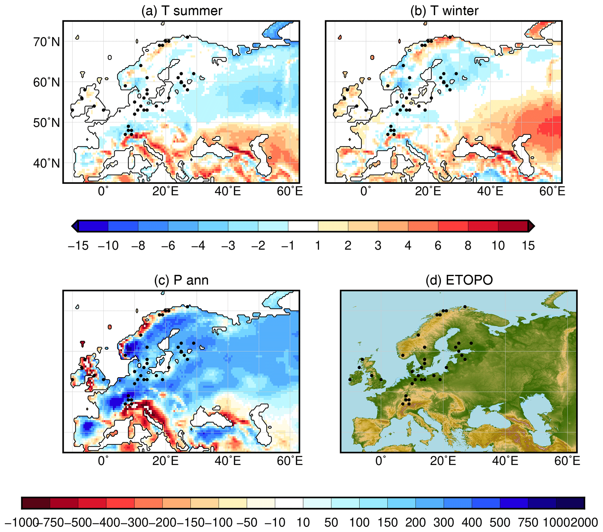
Figure A1Difference between the pre-industrial climate simulated by MPI-ESM1.2 (bilinearly remapped on a 0.5 grid) and the CRU TS 4.0 dataset (1901–1930) (Harris et al., 2020) chosen as the basic state for the LPJ-GUESS climate forcing. Differences in summer temperature [K] (a), winter temperature [K] (b), and annual mean precipitation [mm yr−1] (c) are shown. (d) Orography (the more brownish, the higher the mountains) based on the ETOPO5 dataset (National Geophysical Data Center, 1993). The black dots display the grid cells for which pollen-based REVEALS estimates of plant cover are available.
Table B1List of chironomid records used in this study. Most of the chironomid-based reconstructions used in this study were extracted from the Temperature 12k Database (Kaufman et al, 2020b). For these records, the dataset name, site information, and references (in the form of the DOI) were taken from the Temp12k_metadata table provided by Kaufman et al. (2020a). For the other reconstructions (marked with *), the information was added accordingly.
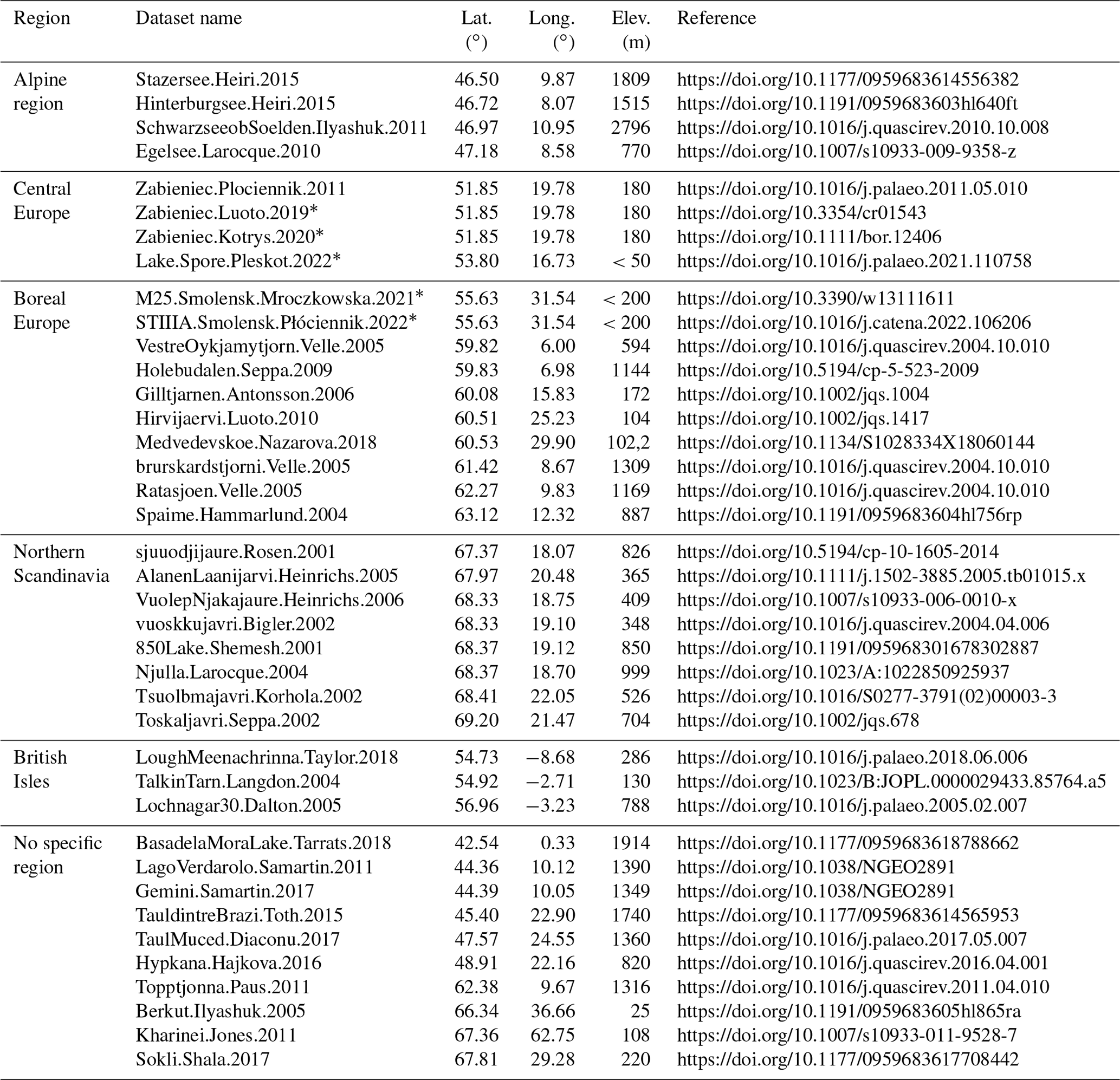
The primary data, i.e. the model code for MPI-ESM, are freely available to the scientific community and can be obtained from MPI-M (see details and contact information at https://mpimet.mpg.de/en/research/modeling, MPI-M, 2023). The simulation (simulation identity: slo0021) will be published soon on the Earth System Grid.
The educational version of LPJ-GUESS is available for download (https://web.nateko.lu.se/lpj-guess/education/, Lund University, 2014), and a fully functional version is available for researchers from the Department of Physical Geography and Ecosystem Sciences at Lund University upon request.
The REVEALS-based vegetation estimates are stored in PANGAEA (Marquer et al., 2019: https://doi.org/10.1594/PANGAEA.900966).
Most of the chironomid-based temperature reconstructions have been downloaded from the Temperature 12k Database (https://doi.org/10.25921/4ry2-g808, Kaufman et al., 2020b).
In addition, secondary data and scripts that may be useful in reproducing the authors' work are archived by the Max Planck Institute for Meteorology and are accessible without any restrictions (https://hdl.handle.net/21.11116/0000-000D-4E03-9, MPG.PuRe, 2023).
All authors planned the study and were involved in the analysis and discussion of the results. AD, AP, LM, and MJG wrote the paper. AP, AD, LM, and AS prepared the figures. All authors commented on, discussed, and edited the final paper.
At least one of the (co-)authors is a guest member of the editorial board of Climate of the Past for the special issue “Past vegetation dynamics and their role in past climate changes”. The peer-review process was guided by an independent editor, and the authors also have no other competing interests to declare.
Publisher's note: Copernicus Publications remains neutral with regard to jurisdictional claims in published maps and institutional affiliations.
This article is part of the special issue “Past vegetation dynamics and their role in past climate changes”. It is not associated with a conference.
This work contributes to the project PalMod, funded by the German Federal Ministry of Education and Research (BMBF), Research for Sustainability initiative (FONA, https://www.fona.de/de/, last access: 25 July 2023). We acknowledge support through the Estonian Research Council and the Swedish Research Council. This study is also a contribution to the strategic research area BECC at Lund University (Biodiversity and Ecosystem Services in a Changing Climate; https://www.becc.lu.se/, last access: 25 July 2023) and the Swedish strategic research area MERGE (ModElling the Regional and Global Earth system; https://www.merge.lu.se/, last access: 25 July 2023). We acknowledge support through the Past Global Change (PAGES) project and its working group LandCover6k (http://pastglobalchanges.org/landcover6k, last access: 25 July 2023) that in turn received support from the Swiss National Science Foundation, the Swiss Academy of Sciences, the US National Science Foundation, and the Chinese Academy of Sciences.
We thank Thomas Kleinen for comments on an earlier version of the paper. We also thank two anonymous reviewers for their constructive comments.
Anne Dallmeyer has been supported by the Bundesministerium für Bildung und Forschung, project PalMod (grant no. 01LP1920A). Anneli Poska received funding by the Estonian Research Competency Council
(grant no. PRG323). Andrea Seim received funding from the Swedish Research Council (Vetenskapsrådet, grant no. 2018-01272). Financial support from the Linnaeus University Faculty of Health and Life Science was received for Marie-José Gaillard.
The article processing charges for this open-access publication were covered by the Max Planck Society.
This paper was edited by Manuel Chevalier and reviewed by two anonymous referees.
Bader, J., Jungclaus, J., Krivova, N., Lorenz, S., Maycock, A., Raddatz, T., Schmidt, H., Toohey, M., Wu, C. J., and Claussen, M.: Global temperature modes shed light on the Holocene temperature conundrum, Nat. Commun., 11, 4726, https://doi.org/10.1038/s41467-020-18478-6, 2020.
Berger, A. L.: Long-term variations of daily insolation and Quaternary climatic changes, J. Atmos. Sci., 35, 2361–2367, https://doi.org/10.1175/1520-0469(1978)035<2362:ltvodi>2.0.co;2, 1978.
Boy, M., Zhou, P., Kurtén, T., Chen, D., Xavier, C., Clusius, P., Roldin, P., Baykara, M., Pichelstorfer, L., Foreback, B., Bäck, J., Petäjä, T., Makkonen, R., Kerminen, V.-M., Pihlatie, M., Aalto, J., and Kulmala, M.: Positive feedback mechanism between biogenic volatile organic compounds and the methane lifetime in future climates, npj Clim. Atmos. Sci., 5, 72, https://doi.org/10.1038/s41612-022-00292-0, 2022.
Braconnot, P., Zhu, D., Marti, O., and Servonnat, J.: Strengths and challenges for transient Mid- to Late Holocene simulations with dynamical vegetation, Clim. Past, 15, 997–1024, https://doi.org/10.5194/cp-15-997-2019, 2019.
Brovkin, V., Raddatz, T., Reick, C. H., Claussen, M., and Gayler, V.: Global biogeophysical interactions between forest and climate, Geophys. Res. Lett., 36, 1–5, https://doi.org/10.1029/2009GL037543, 2009.
Brovkin, V., Lorenz, S., Raddatz, T., Ilyina, T., Stemmler, I., Toohey, M., and Claussen, M.: What was the source of the atmospheric CO2 increase during the Holocene?, Biogeosciences, 16, 2543–2555, https://doi.org/10.5194/bg-16-2543-2019, 2019.
Cao, X., Tian, F., Li, F., Gaillard, M.-J., Rudaya, N., Xu, Q., and Herzschuh, U.: Pollen-based quantitative land-cover reconstruction for northern Asia covering the last 40 ka cal BP, Clim. Past, 15, 1503–1536, https://doi.org/10.5194/cp-15-1503-2019, 2019.
Čížková, H., Květ, J., Comín, F. A., Laiho, R., Pokorný, J., and Pithart, D.: Actual state of European wetlands and their possible future in the context of global climate change, Aquat. Sci., 75, 3–26, https://doi.org/10.1007/s00027-011-0233-4, 2013.
Dallmeyer, A., Claussen, M., Lorenz, S. J., and Shanahan, T.: The end of the African humid period as seen by a transient comprehensive Earth system model simulation of the last 8000 years, Clim. Past, 16, 117–140, https://doi.org/10.5194/cp-16-117-2020, 2020.
Dallmeyer, A., Claussen, M., Lorenz, S. J., Sigl, M., Toohey, M., and Herzschuh, U.: Holocene vegetation transitions and their climatic drivers in MPI-ESM1.2, Clim. Past, 17, 2481–2513, https://doi.org/10.5194/cp-17-2481-2021, 2021.
Dallmeyer, A., Kleinen, T., Claussen, M., Weitzel, N., Cao, X., and Herzschuh, U.: The deglacial forest conundrum, Nat. Commun., 13, 6035, https://doi.org/10.1038/s41467-022-33646-6, 2022.
Davis, B. A. S., Collins, P. M., and Kaplan, J. O. The age and post-glacial development of the modern European vegetation: a plant functional approach based on pollen data, Veg. Hist. Archaeobot., 2, 303–317, https://doi.org/10.1007/s00334-014-0476-9, 2015.
Dawson, A., Cao, X., Chaput, M., Hopla, E., Li, Furong, Edwards, M., Fyfe, R., Gajewski, K., Goring, S. J., Herzschuh, Ulrike, Mazier, F., Sugita, S., Williams, J. W., Xu, Q., and Gaillard, M.-J.: Finding the magnitude of human-induced Northern Hemisphere land-cover transformation between 6 and 0.2 ka BP, PAGES Mag., 26, 34–35, https://doi.org/10.22498/pages.26.1.34, 2018.
Eggermont, H. and Heiri, O.: The chironomid-temperature relationship: expression in nature and palaeoenvironmental implications, Biol. Rev., 87, 430–456, https://doi.org/10.1111/j.1469-185X.2011.00206.x, 2012.
Fyfe, R. M., Roberts, C. N., and Woodbridge, J.: A pollen-based pseudo-biomisation approach to anthropogenic land cover change, Holocene, 20, 1165–1171, 2010.
Fyfe, R. M., Twiddle, C., Sugita, S., Gaillard, M.-J., Barratt, P., Caseldine, C. J., Dodson, J., Edwards, K. J., Farrell, M., Froyd, C., Grant, M. J., Huckerby, E., Innes, J. B., Shaw, H., and Waller, M.: The Holocene vegetation cover of Britain and Ireland: overcoming problems of scale and discerning patterns of openness, Quaternary Sci. Rev. 73, 132–148, https://doi.org/10.1016/j.quascirev.2013.05.014, 2013.
Gaillard, M.-J. and LandCover6k Interim Steering Group members: LandCover6k: Global anthropogenic land-cover change and its role in past climate, PAGES Mag., 23, 38–39, https://doi.org/10.22498/pages.23.1.38, 2015.
Gaillard, M.-J., Sugita, S., Mazier, F., Trondman, A. K., Broström, A., Hickler, T., Kaplan, J. O., Kjellström, E., Kokfelt, U., Kuneš, P., Lemmen, C., Miller, P., Olofsson, J., Poska, A., Rundgren, M., Smith, B., Strandberg, G., Fyfe, R., Nielsen, A. B., Alenius, T., Balakauskas, L., Barnekow, L., Birks, H. J. B., Bjune, A., Björkman, L., Giesecke, T., Hjelle, K., Kalnina, L., Kangur, M., Van Der Knaap, W. O., Koff, T., Lageras, P., Latałowa, M., Leydet, M., Lechterbeck, J., Lindbladh, M., Odgaard, B., Peglar, S., Segerström, U., Von Stedingk, H., and Seppä, H.: Holocene land-cover reconstructions for studies on land cover-climate feedbacks, Clim.e Past, 6, 483–499, https://doi.org/10.5194/cp-6-483-2010, 2010.
Gallego-Sala, A. V., Charman, D. J., Harrison, S. P., Li, G., and Prentice, I. C.: Climate-driven expansion of blanket bogs in Britain during the Holocene, Clim. Past, 12, 129–136, https://doi.org/10.5194/cp-12-129-2016, 2016.
Garreta, V., Miller, P. A., Guiot, J., Hély, C., Brewer, S., Sykes, M. T., and Litt, T.: A method for climate and vegetation reconstruction through the inversion of a dynamic vegetation model, Clim. Dynam., 35, 371–389, https://doi.org/10.1007/s00382-009-0629-1, 2010.
Giesecke, T., Brewer, S., Finsinger, W., Leydet, M., and Bradshaw, R. H. W.: Patterns and dynamics of European vegetation change over the last 15,000 years, J. Biogeogr., 44, 1441–1456, https://doi.org/10.1111/jbi.12974, 2017.
Githumbi, E., Fyfe, R., Gaillard, M.-J., Trondman, A.-K., Mazier, F., Nielsen, A.-B., Poska, A., Sugita, S., Woodbridge, J., Azuara, J., Feurdean, A., Grindean, R., Lebreton, V., Marquer, L., Nebout-Combourieu, N., Stančikaitė, M., Tanţău, I., Tonkov, S., Shumilovskikh, L., and LandClimII data contributors: European pollen-based REVEALS land-cover reconstructions for the Holocene: methodology, mapping and potentials, Earth Syst. Sci. Data, 14, 1581–1619, https://doi.org/10.5194/essd-14-1581-2022, 2022a.
Githumbi, E., Pirzamanbein, B., Lindström, J., Poska, A., Fyfe, R., Mazier, F., Nielsen, A. B., Sugita, S., Trondman, A.-K., Woodbridge, J., and Gaillard, M.-J.: Pollen-Based Maps of Past Regional Vegetation Cover in Europe Over 12 Millennia – Evaluation and Potential, Front. Ecol. Evol., 10, 2022, https://doi.org/10.3389/fevo.2022.795794, 2022b.
Harper, A. B., Powell, T., Cox, P. M., House, J., Huntingford, C., Lenton, T. M., Sitch, S., Burke, E., Chadburn, S. E., Collins, W. J., Comyn-Platt, E., Daioglou, V., Doelman, J. C., Hayman, G., Robertson, E., van Vuuren, D., Wiltshire, A., Webber, C. P., Bastos, A., Boysen, L., Ciais, P., Devaraju, N., Jain, A. K., Krause, A., Poulter, B., and Shu, S.: Land-use emissions play a critical role in land-based mitigation for Paris climate targets, Nat. Commun., 9, 2938, https://doi.org/10.1038/s41467-018-05340-z, 2018.
Harris, I., Osborn, T. J., Jones, P., and Lister, D.: Version 4 of the CRU TS monthly high-resolution gridded multivariate climate dataset, Sci. Data, 7, 109, https://doi.org/10.1038/s41597-020-0453-3, 2020.
Harrison, S. P., Jolly, D., Laarif, F., Abe-Ouchi, A., Dong, B., Herterich, K., Hewitt, C., Joussaume, S., Kutzbach, J. E., Mitchell, J., De Noblet, N., and Valdes, P.: Intercomparison of simulated global vegetation distributions in response to 6 kyr BP orbital forcing, J. Climate, 11, 2721–2742, 1998.
Harrison, S. P., Gaillard, M.-J., Stocker, B. D., Vander Linden, M., Klein Goldewijk, K., Boles, O., Braconnot, P., Dawson, A., Fluet-Chouinard, E., Kaplan, J. O., Kastner, T., Pausata, F. S. R., Robinson, E., Whitehouse, N. J., Madella, M., and Morrison, K. D.: Development and testing scenarios for implementing land use and land cover changes during the Holocene in Earth system model experiments, Geosci. Model Dev., 13, 805–824, https://doi.org/10.5194/gmd-13-805-2020, 2020.
Hellman, S., Gaillard, M.-J., Broström, A., and Sugita, S.: The REVEALS model, a new tool to estimate past regional plant abundance from pollen data in large lakes: validation in southern Sweden, J. Quaternary Sci., 23, 21–42, https://doi.org/10.1002/jqs.1126, 2008a.
Hellman, S. E. V., Gaillard, M., Broström, A., and Sugita, S.: Effects of the sampling design and selection of parameter values on pollen-based quantitative reconstructions of regional vegetation: a case study in southern Sweden using the REVEALS model, Veget. Hist. Archaeobot., 17, 445–459, https://doi.org/10.1007/s00334-008-0149-7, 2008b.
Hengl, T., Walsh, M. G., Sanderman, J., Wheeler, I., Harrison, S. P., and Prentice, I. C.: Global mapping of potential natural vegetation: an assessment of machine learning algorithms for estimating land potential, Peer J., 6, e5457, https://doi.org/10.7717/peerj.5457, 2018.
Hickler, T., Vohland, K., Feehan, J., Miller, P. A., Smith, B., Costa, L., Giesecke, T., Fronzek, S., Carter, T. R., Cramer, W., Kühn, I., and Sykes, M. T.: Projecting the future distribution of European potential natural vegetation zones with a generalized, tree species-based dynamic vegetation model: Future changes in European vegetation zones, Global Ecol. Biogeogr., 21, 50–63, https://doi.org/10.1111/j.1466-8238.2010.00613.x, 2012.
Hopcroft, P. O., Valdes, P. J., Harper, A. B., and Beerling, D. J.: Multi vegetation model evaluation of the Green Sahara climate regime, Geophys. Res. Lett., 44, 6804–6813, https://doi.org/10.1002/2017GL073740, 2017.
Huang, B., Hu, X., Fuglstad, G.-A., Zhou, X., Zhao, W., and Cherubini, F.: Predominant regional biophysical cooling from recent land cover changes in Europe, Nat. Commun., 11, 1066, https://doi.org/10.1038/s41467-020-14890-0, 2020.
Hurtt, G. C., Chini, L., Sahajpal, R., Frolking, S., Bodirsky, B. L., Calvin, K., Doelman, J. C., Fisk, J., Fujimori, S., Klein Goldewijk, K., Hasegawa, T., Havlik, P., Heinimann, A., Humpenöder, F., Jungclaus, J., Kaplan, J. O., Kennedy, J., Krisztin, T., Lawrence, D., Lawrence, P., Ma, L., Mertz, O., Pongratz, J., Popp, A., Poulter, B., Riahi, K., Shevliakova, E., Stehfest, E., Thornton, P., Tubiello, F. N., van Vuuren, D. P., and Zhang, X.: Harmonization of global land use change and management for the period 850–2100 (LUH2) for CMIP6, Geosci. Model Dev., 13, 5425–5464, https://doi.org/10.5194/gmd-13-5425-2020, 2020.
Kaplan, J., Krumhardt, K., Gaillard, M.-J., Sugita, S., Trondman, A.-K., Fyfe, R., Marquer, L., Mazier, F., and Nielsen, A.: Constraining the Deforestation History of Europe: Evaluation of Historical Land Use Scenarios with Pollen-Based Land Cover Reconstructions, Land, 6, 91, https://doi.org/10.3390/land6040091, 2017.
Kaplan, J. O., Krumhardt, K. M., and Zimmermann, N.: The prehistoric and preindustrial deforestation of Europe, Quaternary Sci. Rev., 28, 3016–3034, https://doi.org/10.1016/j.quascirev.2009.09.028, 2009.
Kaufman, D., McKay, N., Routson, C., Erb, M., Davis, B., Heiri, O., Jaccard, S., Tierney, J., Dätwyler, C., Axford, Y., Brussel, T., Cartapanis, O., Chase, B., Dawson, A., de Vernal, A., Engels, S., Jonkers, L., Marsicek, J., Moffa-Sánchez, P., Morrill, C., Orsi, A., Rehfeld, K., Saunders, K., Sommer, P. S., Thomas, E., Tonello, M., Tóth, M., Vachula, R., Andreev, A., Bertrand, S., Biskaborn, B., Bringué, M., Brooks, S., Caniupán, M., Chevalier, M., Cwynar, L., Emile-Geay, J., Fegyveresi, J., Feurdean, A., Finsinger, W., Fortin, M. C., Foster, L., Fox, M., Gajewski, K., Grosjean, M., Hausmann, S., Heinrichs, M., Holmes, N., Ilyashuk, B., Ilyashuk, E., Juggins, S., Khider, D., Koinig, K., Langdon, P., Larocque-Tobler, I., Li, J., Lotter, A., Luoto, T., Mackay, A., Magyari, E., Malevich, S., Mark, B., Massaferro, J., Montade, V., Nazarova, L., Novenko, E., Pařil, P., Pearson, E., Peros, M., Pienitz, R., Płóciennik, M., Porinchu, D., Potito, A., Rees, A., Reinemann, S., Roberts, S., Rolland, N., Salonen, S., Self, A., Seppä, H., Shala, S., St-Jacques, J. M., Stenni, B., Syrykh, L., Tarrats, P., Taylor, K., van den Bos, V., Velle, G., Wahl, E., Walker, I., Wilmshurst, J., Zhang, E., and Zhilich, S.: A global database of Holocene paleotemperature records, Sci. Data, 7, 115, https://doi.org/10.1038/s41597-020-0445-3, 2020a.
Kaufman, D. S., McKay, N. P., and Routson, C.: NOAA/WDS Paleoclimatology – Temperature 12k Database, NOAA National Centers for Environmental Information [data set], https://doi.org/10.25921/4ry2-g808, 2020b.
Kleinen, T., Tarasov, P., Brovkin, V., Andreev, A., and Stebich, M.: Comparison of modeled and reconstructed changes in forest cover through the past 8000 years, Holocene, 21, 723–734, https://doi.org/10.1177/0959683610386980, 2011.
Klein Goldewijk, K., Beusen, A., Doelman, J., and Stehfest, E.: Anthropogenic land use estimates for the Holocene – HYDE 3.2, Earth Syst. Sci. Data, 9, 927–953, https://doi.org/10.5194/essd-9-927-2017, 2017.
Köhler, P.: Interactive comment on “What was the source of the atmospheric CO2 increase during the Holocene?” by Victor Brovkin et al., Biogeosciences Discuss., https://doi.org/10.5194/bg-2019-64-SC1, 2019.
Köppen, W.: Das geographische System der Klimate, in: Handbuch der Klimatologie, Band. 1, Teil C, Verlag von Gebrüder Borntraeger, Berlin, https://koeppen-geiger.vu-wien.ac.at/pdf/Koppen_1936.pdf (last access: 25 July 2023), 1936.
Kotrys, B., Płóciennik, M., Sydor, P., and Brooks, S. J.: Expanding the Swiss-Norwegian chironomid training set with Polish data, Boreas, 49, 89–107, https://doi.org/10.1111/bor.12406, 2020.
Krivova, N. A., Solanki, S. K., and Unruh, Y. C.: Towards a long-term record of solar total and spectral irradiance, J. Atmos. Sol.-Terr. Phy., 73, 223–234, https://doi.org/10.1016/j.jastp.2009.11.013, 2011.
Li, F., Gaillard, M.-J., Cao, X., Herzschuh, U., Sugita, S., Tarasov, P. E., Wagner, M., Xu, Q., Ni, J., Wang, W., Zhao, Y., An, C., Beusen, A. H. W., Chen, F., Feng, Z., Goldewijk, C. G. M. K., Huang, X., Li, Y., Li, Y., Liu, H., Sun, A., Yao, Y., Zheng, Z., and Jia, X.: Towards quantification of Holocene anthropogenic land-cover change in temperate China: A review in the light of pollen-based REVEALS reconstructions of regional plant cover, Earth-Sci. Rev., 203, 103119, https://doi.org/10.1016/j.earscirev.2020.103119, 2020.
Li, F., Gaillard, M.-J., Cao, X., Herzschuh, U., Sugita, S., Ni, J., Zhao, Y., An, C., Huang, X., Li, Y., Liu, H., Sun, A., and Yao, Y.: Gridded pollen-based Holocene regional plant cover in temperate and northern subtropical China suitable for climate modelling, Earth Syst. Sci. Data, 15, 95–112, https://doi.org/10.5194/essd-15-95-2023, 2023.
Lindeskog, M., Arneth, A., Bondeau, A., Waha, K., Seaquist, J., Olin, S., and Smith, B.: Implications of accounting for land use in simulations of ecosystem carbon cycling in Africa, Earth Syst. Dynam., 4, 385–407, https://doi.org/10.5194/esd-4-385-2013, 2013.
Lu, Z., Miller, P. A., Zhang, Q., Zhang, Q., Wårlind, D., Nieradzik, L., Sjolte, J., and Smith, B.: Dynamic Vegetation Simulations of the Mid-Holocene Green Sahara, Geophys. Res. Lett., 45, 8294–8303, https://doi.org/10.1029/2018GL079195, 2018.
Lu, Z., Zhang, Q., Miller, P. A., Zhang, Q., Berntell, E., and Smith, B.: Impacts of Large-Scale Sahara Solar Farms on Global Climate and Vegetation Cover, Geophys. Res. Lett., 48, e2020GL090789, https://doi.org/10.1029/2020GL090789, 2021.
Lund University: LPJ-GUESS Education, https://web.nateko.lu.se/lpj-guess/education/ (last access: 25 July 2023), 2014.
Luoto, T., Kotrys, B., and Płóciennik, M.: East European chironomid-based calibration model for past summer temperature reconstructions, Clim. Res., 77, 63–76, https://doi.org/10.3354/cr01543, 2019.
Marquer, L., Gaillard, M.-J., Sugita, S., Trondman, A.-K., Mazier, F., Nielsen, A. B., Fyfe, R. M., Odgaard, B. V., Alenius, T., Birks, H. J. B., Bjune, A. E., Christiansen, J., Dodson, J., Edwards, K. J., Giesecke, T., Herzschuh, U., Kangur, M., Lorenz, S., Poska, A., Schult, M., and Seppä, H.: Holocene changes in vegetation composition in northern Europe: why quantitative pollen-based vegetation reconstructions matter, Quaternary Sci. Rev., 90, 199–216, https://doi.org/10.1016/j.quascirev.2014.02.013, 2014.
Marquer, L., Gaillard, M.-J., Sugita, S., Poska, A., Trondman, A.-K., Mazier, F., Nielsen, A. B., Fyfe, R. M., Jönsson, A. M., Smith, B., Kaplan, J. O., Alenius, T., Birks, H. J. B., Bjune, A. E., Christiansen, J., Dodson, J., Edwards, K. J., Giesecke, T., Herzschuh, U., Kangur, M., Koff, T., Latałowa, M., Lechterbeck, J., Olofsson, J., and Seppä, H.: Quantifying the effects of land use and climate on Holocene vegetation in Europe, Quaternary Sci. Rev., 171, 20–37, https://doi.org/10.1016/j.quascirev.2017.07.001, 2017.
Marquer, L., Dallmeyer, A., Poska, A., Pongratz, J., Smith, B., and Gaillard, M.-J.: Modeling past human-induced vegetation change is a challenge – the case of Europe, Past Global Change. Mag., 26, 12–13, https://doi.org/10.22498/pages.26.1.12, 2018.
Marquer, L., Gaillard, M.-J., Sugita, S., Poska, A., Trondman, A.-K., Mazier, F., Nielsen, A. B., Fyfe, R. M., Jönsson, A. M., Smith, B., Kaplan, J. O., Alenius, T., Birks, H. J. B., Bjune, A. E., Christiansen, J., Dodson, J., Edwards, K. J., Giesecke, T., Herzschuh, U., Kangur, M., Koff, T., Latalowa, M., Lechterbeck, J., Olofsson, J., and Seppä, H.: Pollen-based REVEALS estimates of plant cover in Europe for 36 grid-cells and the last 11700 years, PANGAEA [data set], https://doi.org/10.1594/PANGAEA.900966, 2019.
Marquer, L., Mazier, F., Sugita, S., Galop, D., Houet, T., Faure, E., Gaillard, M.-J., Haunold, S., de Munnik, N., Simonneau, A., De Vleeschouwer, F., and Le Roux, G.: Pollen-based reconstruction of Holocene land-cover in mountain regions: Evaluation of the Landscape Reconstruction Algorithm in the Vicdessos valley, northern Pyrenees, France, Quaternary Sci. Rev., 228, 106049, https://doi.org/10.1016/j.quascirev.2019.106049, 2020.
Mauritsen, T., Bader, J., Becker, T., Behrens, J., Bittner, M., Brokopf, R., Brovkin, V., Claussen, M., Crueger, T., Esch, M., Fast, I., Fiedler, S., Fläschner, D., Gayler, V., Giorgetta, M., Goll, D. S., Haak, H., Hagemann, S., Hedemann, C., Hohenegger, C., Ilyina, T., Jahns, T., Jimenéz-de-la-Cuesta, D., Jungclaus, J., Kleinen, T., Kloster, S., Kracher, D., Kinne, S., Kleberg, D., Lasslop, G., Kornblueh, L., Marotzke, J., Matei, D., Meraner, K., Mikolajewicz, U., Modali, K., Möbis, B., Müller, W. A., Nabel, J. E. M. S., Nam, C. C. W., Notz, D., Nyawira, S. S., Paulsen, H., Peters, K., Pincus, R., Pohlmann, H., Pongratz, J., Popp, M., Raddatz, T. J., Rast, S., Redler, R., Reick, C. H., Rohrschneider, T., Schemann, V., Schmidt, H., Schnur, R., Schulzweida, U., Six, K. D., Stein, L., Stemmler, I., Stevens, B., von Storch, J. S., Tian, F., Voigt, A., Vrese, P., Wieners, K. H., Wilkenskjeld, S., Winkler, A., and Roeckner, E.: Developments in the MPI-M Earth System Model version 1.2 (MPI-ESM1.2) and Its Response to Increasing CO2, J. Adv. Model. Earth Syst., 11, 998–1038, https://doi.org/10.1029/2018MS001400, 2019.
Mazier, F., Gaillard, M.-J., Kuneš, P., Sugita, S., Trondman, A.-K., and Broström, A.: Testing the effect of site selection and parameter setting on REVEALS-model estimates of plant abundance using the Czech Quaternary Palynological Database, Rev. Palaeobot. Palynol., 187, 38–49, https://doi.org/10.1016/j.revpalbo.2012.07.017, 2012.
Miller, P. A., Giesecke, T., Hickler, T., Bradshaw, R. H. W., Smith, B., Seppä, H., Valdes, P. J., and Sykes, M. T.: Exploring climatic and biotic controls on Holocene vegetation change in Fennoscandia, J. Ecol., 96, 247–259, https://doi.org/10.1111/j.1365-2745.2007.01342.x, 2008.
Monsi, M.: On the Factor Light in Plant Communities and its Importance for Matter Production, Ann. Bot., 95, 549–567, https://doi.org/10.1093/aob/mci052, 2004.
Monsi, M. and Saeki, T.: Über den Lichtfaktor in den Pflanzengesellschaften und seine Bedeutung für die Stoffproduktion, Jpn. J. Bot., 14, 22–52, 1953.
MPG.PuRe: The challenge of comparing pollen-based quantitative vegetation reconstructions with outputs from vegetation models – a European perspective, Publication Repository of the Max-Planck-Society, https://hdl.handle.net/21.11116/0000-000D-4E03-9 (last access: 21 June 2023), 2023.
MPI-M: Climate Modeling at the Max Planck Institute for Meteorology, official webpage of the Max Planck Institute for Meteorology, https://mpimet.mpg.de/en/research/modeling (last access: 25 July 2023), 2023.
Müller, C., Franke, J., Jägermeyr, J., Ruane, A. C., Elliott, J., Moyer, E., Heinke, J., Falloon, P. D., Folberth, C., Francois, L., Hank, T., Izaurralde, R. C., Jacquemin, I., Liu, W., Olin, S., Pugh, T. A. M., Williams, K., and Zabel, F.: Exploring uncertainties in global crop yield projections in a large ensemble of crop models and CMIP5 and CMIP6 climate scenarios, Environ. Res. Lett., 16, 034040, https://doi.org/10.1088/1748-9326/abd8fc, 2021.
National Geophysical Data Center: 5-minute Gridded Global Relief Data (ETOPO5), https://data.nodc.noaa.gov/cgi-bin/iso?id=gov.noaa.ngdc.mgg.dem:3141 (last access: 25 July 2023), 1993.
Nielsen, A. B., Giesecke, T., Theuerkauf, M., Feeser, I., Behre, K.-E., Beug, H.-J., Chen, S.-H., Christiansen, J., Dörfler, W., Endtmann, E., Jahns, S., de Klerk, P., Kühl, N., Latałowa, M., Odgaard, B. V., Rasmussen, P., Stockholm, J. R., Voigt, R., Wiethold, J., and Wolters, S.: Quantitative reconstructions of changes in regional openness in north-central Europe reveal new insights into old questions, Quaternary Sci. Rev., 47, 131–149, https://doi.org/10.1016/j.quascirev.2012.05.011, 2012.
Olofsson, J. and Hickler, T.: Effects of human land-use on the global carbon cycle during the last 6,000 years, Veget. Hist. Archaeobot., 17, 605–615, https://doi.org/10.1007/s00334-007-0126-6, 2008.
Piao, S., Sitch, S., Ciais, P., Friedlingstein, P., Peylin, P., Wang, X., Ahlström, A., Anav, A., Canadell, J. G., Cong, N., Huntingford, C., Jung, M., Levis, S., Levy, P. E., Li, J., Lin, X., Lomas, M. R., Lu, M., Luo, Y., Ma, Y., Myneni, R. B., Poulter, B., Sun, Z., Wang, T., Viovy, N., Zaehle, S., and Zeng, N.: Evaluation of terrestrial carbon cycle models for their response to climate variability and to CO2 trends, Global Change Biol., 19, 2117–2132, https://doi.org/10.1111/gcb.12187, 2013.
Pirzamanbein, B., Lindström, J., Poska, A., Sugita, S., Trondman, A. K., Fyfe, R., Mazier, F., Nielsen, A. B., Kaplan, J. O., Bjune, A. E., Birks, H. J. B., Giesecke, T., Kangur, M., Latałowa, M., Marquer, L., Smith, B., and Gaillard, M. J.: Creating spatially continuous maps of past land cover from point estimates: A new statistical approach applied to pollen data, Ecol. Complex., 20, 127–141, https://doi.org/10.1016/j.ecocom.2014.09.005, 2014.
Pirzamanbein, B., Poska, A., and Lindström, J.: Bayesian reconstruction of past land cover from pollen data: Model robustness and sensitivity to auxiliary variables, Earth Space Sci., 7, e2018EA00057, https://doi.org/10.1029/2018EA000547, 2020.
Pleskot, K., Apolinarska, K., Cwynar, L. C., Kotrys, B., and Lamentowicz, M.: The late-Holocene relationship between peatland water table depth and summer temperature in northern Poland, Palaeogeogr. Palaeocl. Palaeoecol., 586, 110758, https://doi.org/10.1016/j.palaeo.2021.110758, 2022.
Płóciennik, M., Self, A., Birks, H. J. B., and Brooks, S. J.: Chironomidae (Insecta: Diptera) succession in Żabieniec bog and its palaeo-lake (central Poland) through the Late Weichselian and Holocene, Palaeogeography, Palaeoclimatology, Palaeoecology, 307, 150–167, https://doi.org/10.1016/j.palaeo.2011.05.010, 2011.
Prentice, I. C.: Multidimensional scaling as a research tool in quaternary palynology: A review of theory and methods, Rev. Palaeobot. Palynol., 31, 71–104, https://doi.org/10.1016/0034-6667(80)90023-8, 1980.
Prentice, I. C.: Pollen representation, source area, and basin size: toward a unified theory of pollen analysis, Quatern. Res., 23, 76–86, 1985.
Prentice, I. C., Sykes, M. T., Lautenschlager, M., Harrison, S. P., Denissenko, O., and Bartlein, P. J.: Modelling Global Vegetation Patterns and Terrestrial Carbon Storage at the Last Glacial Maximum, Global Ecol. Biogeogr. Lett., 3, 67–76, https://doi.org/10.2307/2997548, 1993.
Reick, C. H., Raddatz, T., Brovkin, V., and Gayler, V.: Representation of natural and anthropogenic land cover change in MPI-ESM: Land Cover in MPI-ESM, J. Adv. Model. Earth Syst., 5, 459–482, https://doi.org/10.1002/jame.20022, 2013.
Reick, C. H., Gayler, V., Goll, D., Hagemann, Stefan Heidkamp, M., Nabel, J., Raddatz, T., Roeckner, E., Schnur, R., and Wilkenskjeld, S.: JSBACH 3 – The land component of the MPI Earth System Model: documentation of version 3.2, Berichte zur Erdsystemforschung,MPI für Meteorologie, Hamburg, https://doi.org/10.17617/2.3279802, 2021.
Roberts, N., Fyfe, R. M., Woodbridge, J., Gaillard, M.-J., Davis, B. A. S., Kaplan, J. O., Marquer, L., Mazier, F., Nielsen, A. B., Sugita, S., Trondman, A.-K., and Leydet, M.: Europe's lost forests: a pollen-based synthesis for the last 11,000 years, Sci. Rep., 8, 716, https://doi.org/10.1038/s41598-017-18646-7, 2018.
Ruddiman, W. F.: The early anthropogenic hypothesis: Challenges and responses, Rev. Geophys., 45, RG4001, https://doi.org/10.1029/2006RG000207, 2007.
Ruddiman, W. F., Ellis, E. C., Kaplan, J. O., and Fuller, D. Q.: Defining the epoch we live in, Science, 348, 38–39, https://doi.org/10.1126/science.aaa7297, 2015.
Serge, M. A., Mazier, F., Fyfe, R., Gaillard, M.-J., Klein, T., Lagnoux, A., Galop, D., Githumbi, E., Mindrescu, M., Nielsen, A. B., et al.: Testing the Effect of Relative Pollen Productivity on the REVEALS Model: A Validated Reconstruction of Europe-Wide Holocene Vegetation, Land, 12, 986, https://doi.org/10.3390/land12050986, 2023.
Sitch, S., Smith, B., Prentice, I. C., Arneth, A., Bondeau, A., Cramer, W., Kaplan, J. O., Levis, S., Lucht, W., Sykes, M. T., Thonicke, K., and Venevsky, S.: Evaluation of ecosystem dynamics, plant geography and terrestrial carbon cycling in the LPJ dynamic global vegetation model: LPJ Dynamic Global Vegetation Model, Global Change Biol., 9, 161–185, https://doi.org/10.1046/j.1365-2486.2003.00569.x, 2003.
Smith, B., Prentice, I. C., and Sykes, M. T.: Representation of vegetation dynamics in the modelling of terrestrial ecosystems: Comparing two contrasting approaches within European climate space: Vegetation dynamics in ecosystem models, Global Ecol. Biogeogr., 10, 621–637, https://doi.org/10.1046/j.1466-822X.2001.t01-1-00256.x, 2001.
Smith, B., Knorr, W., Widlowski, J.-L., Pinty, B., and Gobron, N.: Combining remote sensing data with process modelling to monitor boreal conifer forest carbon balances, Forest Ecol. Manage., 255, 3985–3994, https://doi.org/10.1016/j.foreco.2008.03.056, 2008.
Smith, B., Wårlind, D., Arneth, A., Hickler, T., Leadley, P., Siltberg, J., and Zaehle, S.: Implications of incorporating N cycling and N limitations on primary production in an individual-based dynamic vegetation model, Biogeosciences, 11, 2027–2054, https://doi.org/10.5194/bg-11-2027-2014, 2014.
Smith, M. C., Singarayer, J. S., Valdes, P. J., Kaplan, J. O., and Branch, N. P.: The biogeophysical climatic impacts of anthropogenic land use change during the Holocene, Clim. Past, 12, 923–941, https://doi.org/10.5194/cp-12-923-2016, 2016.
Strandberg, G., Kjellström, E., Poska, A., Wagner, S., Gaillard, M.-J., Trondman, A.-K., Mauri, A., Davis, B. A. S., Kaplan, J. O., Birks, H. J. B., Bjune, A. E., Fyfe, R., Giesecke, T., Kalnina, L., Kangur, M., van der Knaap, W. O., Kokfelt, U., Kuneš, P., Latałowa, M., Marquer, L., Mazier, F., Nielsen, A. B., Smith, B., Seppä, H., and Sugita, S.: Regional climate model simulations for Europe at 6 and 0.2 k BP: sensitivity to changes in anthropogenic deforestation, Clim. Past, 10, 661–680, https://doi.org/10.5194/cp-10-661-2014, 2014.
Strandberg, G., Lindström, J., Poska, A., Zhang, Q., Fyfe, R., Githumbi, E., Kjellström, E., Mazier, F., Nielsen, A. B., Sugita, S., Trondman, A.-K., Woodbridge, J., and Gaillard, M.-J.: Mid-Holocene European climate revisited: New high-resolution regional climate model simulations using pollen-based land-cover, Quaternary Sci. Rev., 281, 107431, https://doi.org/10.1016/j.quascirev.2022.107431, 2022.
Strandberg, G., Chen, J., Fyfe, R., Kjellström, E., Lindström, J., Poska, A., Zhang, Q., and Gaillard, M.-J.: Did the Bronze Age deforestation of Europe affect its climate? A regional climate-model study using pollen-based land-cover reconstructions, Clim. Past Discuss. [preprint], https://doi.org/10.5194/cp-2023-17, in review, 2023.
Sugita, S.: Theory of quantitative reconstruction of vegetation I: pollen from large sites REVEALS regional vegetation composition, Holocene, 17, 229–241, https://doi.org/10.1177/0959683607075837, 2007.
Sugita, S., Parshall, T., Calcote, R., and Walker, K.: Testing the Landscape Reconstruction Algorithm for spatially explicit reconstruction of vegetation in northern Michigan and Wisconsin, Quatern. Res., 74, 289–300, https://doi.org/10.1016/j.yqres.2010.07.008, 2010.
Sun, Y., Xu, Q., Gaillard, M.-J., Zhang, S., Li, D., Li, M., Li, Y., Li, X., and Xiao, J.: Pollen-based reconstruction of total land-cover change over the Holocene in the temperate steppe region of China: An attempt to quantify the cover of vegetation and bare ground in the past using a novel approach, Catena, 214, 106307, https://doi.org/10.1016/j.catena.2022.106307, 2022.
Toohey, M. and Sigl, M.: Volcanic stratospheric sulfur injections and aerosol optical depth from 500 BCE to 1900 CE, Earth Syst. Sci. Data, 9, 809–831, https://doi.org/10.5194/essd-9-809-2017, 2017.
Trondman, A., Gaillard, M., Mazier, F., Sugita, S., and Fyfe, R.: Pollen-based quantitative reconstructions of Holocene regional vegetation cover (plant-functional types and land-cover types) in Europe suitable for climate modelling, Global Change Biol., 46, 676–697, https://doi.org/10.1111/gcb.12737, 2015.
Trondman, A.-K., Gaillard, M.-J., Sugita, S., Björkman, L., Greisman, A., Hultberg, T., Lagerås, P., Lindbladh, M., and Mazier, F.: Are pollen records from small sites appropriate for REVEALS model-based quantitative reconstructions of past regional vegetation? An empirical test in southern Sweden, Veget. Hist. Archaeobot., 25, 131–151, https://doi.org/10.1007/s00334-015-0536-9, 2016.
University of East Anglia Climatic Research Unit (CRU), Harris, I. C., and Jones, P. D.: CRU TS4.00: Climatic Research Unit (CRU) Time-Series (TS) version 4.00 of high resolution gridded data of month-by-month variation in climate (Jan. 1901–Dec. 2015), https://catalogue.ceda.ac.uk/uuid/edf8febfdaad48abb2cbaf7d7e846a86 (last access: 25 July 2023), 2017.
Velle, G., Brodersen, K. P., Birks, H. J. B., and Willassen, E.: Midges as quantitative temperature indicator species: Lessons for palaeoecology, Holocene, 20, 989–1002, https://doi.org/10.1177/0959683610365933, 2010.
Williams, J. W. and Jackson, S. T.: Novel climates, no-analog communities, and ecological surprises, Front. Ecol. Environ., 5, 475–482, https://doi.org/10.1890/070037, 2007.
Williamson, P.: Emissions reduction: Scrutinize CO2 removal methods, Nature, 530, 153–155, https://doi.org/10.1038/530153a, 2016.
Wohlfahrt, J., Harrison, S. P., Braconnot, P., Hewitt, C. D., Kitoh, A., Mikolajewicz, U., Otto-Bliesner, B. L., and Weber, S. L.: Evaluation of coupled ocean-atmosphere simulations of the mid-Holocene using palaeovegetation data from the northern hemisphere extratropics, Clim. Dynam., 31, 871–890, 2008.
Wolf, A., Callaghan, T. V., and Larson, K.: Future changes in vegetation and ecosystem function of the Barents Region, Climatic Change, 87, 51–73, https://doi.org/10.1007/s10584-007-9342-4, 2008.
Wramneby, A., Smith, B., and Samuelsson, P.: Hot spots of vegetation-climate feedbacks under future greenhouse forcing in Europe, J. Geophys. Res., 115, D21119, https://doi.org/10.1029/2010JD014307, 2010.
- Abstract
- Introduction
- Methods
- Results
- Discussion
- Summary and conclusions
- Appendix A: Evaluation of the PI climate simulated by MPI-ESM1.2
- Appendix B: List of the chironomid records used in this study
- Code and data availability
- Author contributions
- Competing interests
- Disclaimer
- Special issue statement
- Acknowledgements
- Financial support
- Review statement
- References