the Creative Commons Attribution 4.0 License.
the Creative Commons Attribution 4.0 License.
 | 18 Jul 2023
Earliest meteorological readings in San Fernando (Cádiz, Spain, 1799–1813)
Nieves Bravo-Paredes
María Cruz Gallego
Ricardo M. Trigo
Cádiz and San Fernando are two towns close to each other with a wealth of meteorological records due to their connection with the Spanish Royal Navy officers and enlightened merchants. Several previous works have already recovered a significant number of meteorological records of interest in these localities. However, more than 40 000 daily meteorological observations recorded at the Royal Observatory of the Spanish Navy (located in San Fernando) during the period 1799–1813 were previously unnoticed; they remained neither digitized nor studied. Here, we have carried out this important task, describing the different steps undertaken to achieve it as well as the results obtained. The dataset is composed of different meteorological variables such as atmospheric pressure, air temperature, precipitation, and state of the sky. As a first step a quality control was carried out to find possible errors in the original data or in the digitization process. Moreover, the antique units were converted to modern units. Also, the metadata and an analysis of the data are described. The dataset is freely available to the scientific community and can be downloaded at https://doi.org/10.5281/zenodo.7104289.
- Article
(7634 KB) - Full-text XML
- BibTeX
- EndNote


Long-term series are very important to better understand the variability in the climate as well as to provide a more robust framework to validate long-term trends and extremes. In this context, early meteorological observations are critical to extend instrumental series, particularly during the 18th and 19th centuries. Therefore, climate data rescue should be a continuous effort as part of a long-term activity (Brönnimann et al., 2018). Recovering early meteorological observations represents a huge effort made by a large number of scientists all over the world. Some important examples of structured international efforts in this line of activity are the Atmospheric Circulation Reconstructions over the Earth (ACRE) (http://www.met-acre.org/, last access: 4 July 2023) and the International Data Rescue (I-DARE) portal (https://www.idare-portal.org/, last access: 4 July 2023). Early meteorological data have also been recovered in Latin America and the Caribbean (Domínguez-Castro et al., 2017), in Canada (Slonosky, 2003), in South Africa (Picas et al., 2019), in Brazil (Farrona et al., 2012), and in Japan (Zaiki et al., 2006).
In Europe, different initiatives have been carried out to retrieve early meteorological data. For example, the ADVICE project reconstructed and analyzed mean sea level pressure (MSLP) data from the 16th century onwards (Jones et al., 1999; Luterbacher et al., 2000). There have been more initiatives such as the IMPROVE (Camuffo and Jones, 2002), HISTALP (Auer et al., 2007), and ERACLIM (https://www.ecmwf.int/en/research/projects/era-clim, last access: 4 July 2023) projects. More recent initiatives include, for example, the CHIMES project, which compiles pre-national weather service observations in Switzerland and makes them available in digital format (Pfister et al., 2019; Brugnara et al., 2020).
In the Iberian Peninsula (hereafter IP), different initiatives in the last 2 decades can be found. For example, Alcoforado et al. (2012) retrieved early Portuguese meteorological measurements from the 18th century, while the SIGN project focused on 19th- and early 20th-century data in Portugal (Morozova and Valente, 2012; Bližňák et al., 2015). Domínguez-Castro et al. (2014) recovered more than 100 000 early meteorological observations prior to 1850 in Spain, and Vaquero et al. (2022) recovered more than 750 000 instrumental meteorological observations from 1826 to the mid-20th century in the Extremadura region (interior SW Iberia), presented in the CliPastExtrem database. In the Bay of Cádiz, there are several initiatives to rescue meteorological data that led to a wide number of publications (Barriendos et al., 2002; Gallego et al., 2007; Rodrigo, 2012; Domínguez-Castro et al., 2014; Wheeler, 1995; Rodrigo, 2019).
Figure 1 summarizes the data retrieved for the cities of Cádiz (references in black) and San Fernando (references in red). The first instrumental data were recovered by Wheeler (1995) using temperature measurements made during astronomical observations (passage of the sun through the Cádiz meridian) in 1776. Barriendos et al. (2002) studied the long records of the Urrutia brothers in Cádiz. Gallego et al. (2007) recovered the meteorological records of the Torre de Vigía at Cádiz. The Royal Observatory of the Spanish Navy (ROA, from the Spanish “Real Instituto y Observatorio de la Armada”; located in San Fernando) has published its meteorological records in annual volumes since 1870. In addition, other short series have been recovered (Rodrigo, 2012, 2019; Domínguez-Castro et al., 2014).
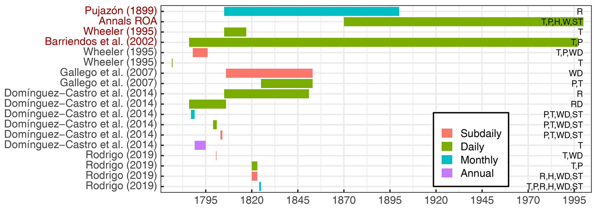
Figure 1Data retrieved for the cities of Cádiz (in black) and San Fernando (in red). The meteorological variables of each dataset are on the right: T – temperature, P – pressure, R – rain, WD – wind direction, H – humidity, RN – rainy days, W – different wind variables, ST – state of the sky.
The main aim of this work is to retrieve the early meteorological observations measured in San Fernando (Cádiz) for the period 1799–1813. Moreover, a quality control and unit changes are carried out to make the data usable. Finally, an analysis of the data is performed. The structure of the paper is as follows: Sect. 2 describes the data and the instruments used; the method used for the quality control and the unit change in the data is presented in Sect. 3; the corresponding results are presented in Sect. 4; and finally, conclusions of this work are presented in Sect. 5. Note that most of the early instrumental records are relatively short series, often even shorter than the one presented here (Brönnimann et al., 2019). Thus, a collection of this kind of series relating to the same place or different places with similar climatic characteristics can be extremely useful for knowing the climate of the past.
The dataset of early meteorological observations recovered here was recorded in the ROA during the period 1799–1813. The ROA is located in the city of San Fernando (Cádiz) in the southwest of the IP (36∘27′42′′ N, 6∘12′20′′ W). Figure 2a shows the location of the city of San Fernando in the IP. Figure 2b shows the location of San Fernando in the Bay of Cádiz. Figure 2c shows the location of the ROA in the city of San Fernando.
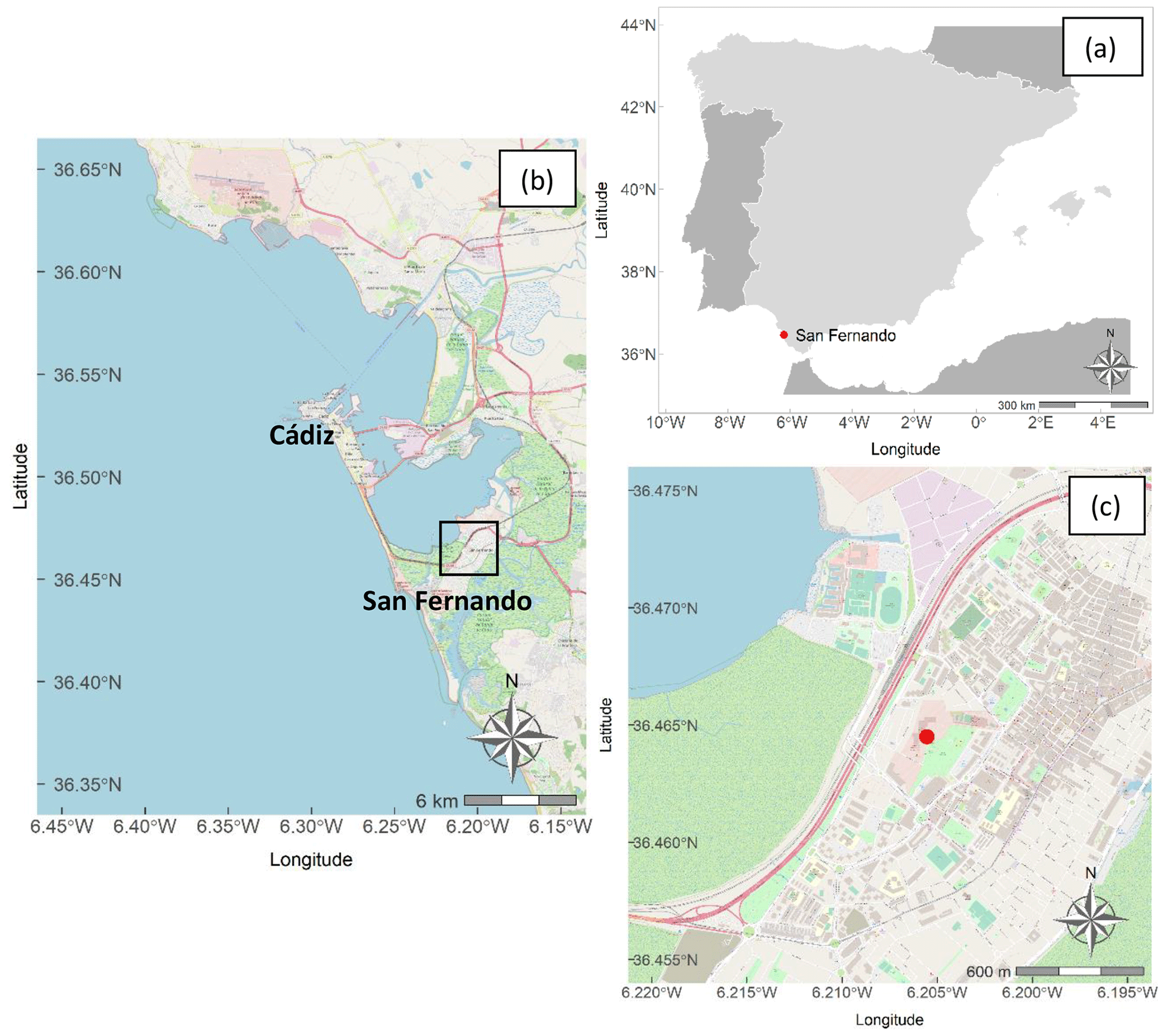
Figure 2(a) The red point shows the location of the city of San Fernando in the IP. (b) The location of San Fernando in the Bay of Cádiz. The box shows the region enlarged in (c). (c) The red point shows the location of the Royal Observatory of the Spanish Navy (ROA) in the city of San Fernando. The maps were created from Instituto Geográfico Nacional (http://www.ign.es, last access: 4 July 2023) and the ggspatial package in R (Dunnington, 2020).
The ROA dataset used here (hereafter SF1799-1813) was obtained within the scope of a larger plan to increase astronomical observations at the observatory starting in 1798. The plan was divided into four classes: tiempo (time), planetas (planets), longitudes terrestres (earth longitudes), and física celeste (celestial physics). Specifically, the observations of SF1799-1813 corresponded to the fourth class (física celeste) (Lafuente and Sellés, 1988). Original data were preserved at the Real Instituto y Observatorio de la Armada in San Fernando in a logbook (catalog number: AH1080).
The ROA observations were made using different instruments and different units. A total of 45 862 discrete observations were made from 1799 to 1813. Figure 3 shows the observation period covered for each meteorological variable of the SF1799-1813 dataset. Pink and green bars correspond to subdaily observations: 06:00, 00:00, 18:00, and 12:00 in pink and 08:00 and 14:00 (all times in local time) in green. Blue bars correspond to daily observations measured at 14:00. Gray bars correspond to monthly observations. Unfortunately, there are two large gaps in the periods 1802–1804 and 1810–1812. The cause of the first gap could be that the work of the officers carried out on the sea was more valued than the scientific work in the ROA. Because of this, there were few officers working at the ROA. Unfortunately, the absence of the officers often means that meteorological observations were not made (Lafuente and Sellés, 1988). The second gap is related to the movement of the observer to the Torre de Zimbrelos. The observer was assigned to watch over the French due to Napoleon's occupation during the Spanish War of Independence, or the Peninsular War. Since there are differences in the observation hours form one period to another, it is possible that there are biases in the daily temperature caused by this fact (Zaiki et al., 2002).
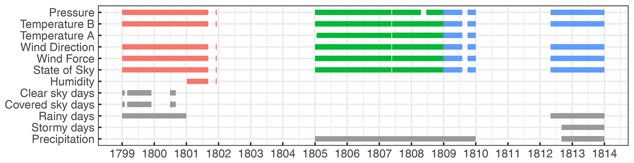
Figure 3Observational period covered by the new dataset for each meteorological variable. Pink, green, and blue bars correspond to subdaily observations: 06:00, 00:00, 18:00, and 12:00 in pink; 08:00 and 14:00 in green; 14:00 in blue. Gray bars correspond to monthly observations.
Additionally, another dataset of the ROA is used for comparison purposes with the SF1799-1813 dataset. This dataset covers the recent period 1997–2021 and can be found at https://datosclima.es/ (last access: last access: 4 July 2023; hereafter SF1997-2021). Finally, a monthly global paleo-reanalysis (EKF400v2) generated to cover the 1600 and 2005 time period by Valler et al. (2021) was used to make comparisons with the SF1799-1813 dataset.
The station elevation appears in the metadata but is different for each period. There are no station elevation data in the metadata for the period 1799–1801. For the period 1805–1809, the station elevation was recorded as 142.5 Burgos feet (1 Burgos foot = 0.2786 m). For the period 1812–1813, the elevation was recorded as 100 Burgos feet above sea level. This last value has been chosen for the period 1799–1801 due to the average of the pressure values for the period 1799–1801 being quite similar to the average of the pressure values for the period 1812–1813. In addition, the observations were registered with the same instruments and could be at the same location. A brief description of each variable is given below.
-
Pressure. Pressure observations were recorded with two different mercury barometers and in different units. For 1799–1801 and 1812–1813, pressure observations were recorded subdaily in English inches with a George Adams barometer. For 1805–1809, pressure observations were recorded subdaily in French inches with a Megnié barometer.
-
Temperature (thermometer attached to the barometer). Mercury barometers typically had a thermometer attached to do the temperature correction for pressure observations. Temperature observations of the thermometers attached to the barometers were recorded subdaily with different thermometers in different units. For 1799–1801 and 1812–1813, the thermometer attached to the George Adams barometer registered subdaily observations in degrees Fahrenheit. For 1805–1809, the thermometer attached to the Megnié barometer recorded subdaily observations in degrees Réaumur.
-
Air temperature. Air temperature was recorded with a Dollond thermometer in degrees Fahrenheit for the period 1805–1809.
-
Wind direction. Wind direction observations were recorded subdaily by following the wind rose directions. The wind rose was divided into 32 directions: N, NxNE, NNE, NExN, NE, NExE, ENE, ExNE, E, ExSE, ESE, SExE, SE, SExS, SSE, SxSE, S, SxSW, SSW, SWxS, SW, SWxW, WSW, WxSW, W, WxNW, WNW, NWxW, NW, NWxN, NNW, NxNW. The term “x” between directions means “by” in English. In the original data, these wind directions were recorded as, for example, “NE1/4E”. In the digitization process, the term “NE1/4E” was replaced by “NExE”.
The prevailing wind direction in the 24 h was recorded for the period 1812–1813, although there is no further indication in the original manuscript.
-
Wind force. Wind force observations were recorded subdaily in textual form using descriptors. García-Herrera et al. (2003) wrote a dictionary to clarify the archaic wind force terms in a comprehensible format. This dictionary was used to check the wind force terms from the original document. Most of the terms for the whole period appear in the dictionary.
The prevailing wind force in the 24 h was recorded for the period 1812–1813.
-
State of the sky. The observers gave a detailed description of the state of the sky subdaily during the period 1799–1801. Clear or covered sky, number of clouds, and rain or other types of precipitation are examples of what usually appears in the description.
The state of the sky has been recorded differently since 1805. The description was summarized in just one word, for example, “clear” to indicate that the sky was cloudless.
The prevailing state of the sky in the 24 h was recorded for the period 1812–1813.
Moreover, the number of clear, covered, rainy, and stormy days was also registered monthly in different periods. Clear, covered, and rainy days were recorded for the period 1799–1800. Rainy and stormy days were recorded for the period 1812–1813.
-
Humidity. There is no information about the humidity in the metadata. The humidity was registered only for the period 6 January–11 December 1801.
-
Precipitation. The precipitation was recorded weekly in Burgos inches (1 Burgos inch = 23.22 mm) for the period 1805–1808 and monthly for the year 1809 and the period 1812–1813.
Data were digitized by key entry from photographs taken from the manuscript. The dataset was analyzed through a basic quality control applied to detect possible errors in the digitization process or suspicious values (Vaquero et al., 2022). Moreover, the units were changed to modern SI units. The steps are described in the following sections.
3.1 Quality control
Digitized data often contain errors as a result of typing an incorrect number in the digital document instead of the actual number in the original document. These errors should be detected and corrected whenever possible. Moreover, quality control could detect suspicious values. These values were digitized correctly. Therefore, it is possible that the observers wrote an incorrect number instead of the correct number (e.g., a maximum daily temperature with lower values than the corresponding minimum daily temperature). Suspicious values detected by quality control are flagged with an asterisk and are not corrected.
A basic quality control was carried out in order to detect possible typos, errors, and suspicious values in the digitization process. The quality control consists of the following.
-
Visual check. Some variables are bounded by upper and/or lower limit values. For example, pressure lines cannot exceed the value of 12. If there are values that exceed this threshold, the values are checked against the original data and corrected.
-
Compare means. The daily and monthly means calculated by the observers were digitized and compared with the means computed from the digitized data. If the means are not equal, the values corresponding to that mean are checked against the original data and corrected whenever a mistake is detected.
-
Extreme values. In order to detect outlier values, the mean ±3 standard deviations is calculated by the authors. Values that exceed this threshold are checked against the original data and corrected if there is an obvious error.
-
Consecutive values. The difference in the values between consecutive days is also calculated. This difference should not exceed a predefined threshold. The threshold is estimated by the mean ± 3 standard deviations of the differences. Values above this threshold could be due to an error, a suspicious value, or an outlier. Values that exceed this threshold are checked against the original data and corrected if it is an error.
The four quality control steps mentioned above were applied to pressure and temperature variables (temperature related to the thermometer attached to the barometer). For the air temperature variable and for the humidity only steps 1, 3, and 4 were applied.
3.2 Unit change
3.2.1 Temperature
Temperature was measured using the Reaumur and Fahrenheit scales in different periods. Temperatures were converted to Celsius using the two following equations: Eq. (1) converts Reaumur to Celsius, while Eq. (2) converts Fahrenheit to Celsius.
3.2.2 Pressure
Pressure was measured in two different length units, English and French inches, in two different periods. Pressure measurements originally registered in inches were converted to meters. Equation (3) is used to convert the English inch to meters. Equation (4) is used to convert the French inch to meters.
Reduction to 0 ∘C
Mercury expands and shrinks depending on the temperature. Therefore, meteorological observations recorded with a mercury barometer should be reduced to 0 ∘C. The following equation gives the density of mercury as a function of temperature:
where α= 0.0001818 K−1 is the volumetric thermal coefficient for mercury at 0 ∘C, ρ0= 13595.1 kg m−3 is the density of mercury at 0 ∘C, and T is the temperature of the thermometer attached to the barometer.
The barometer scale could expand due to temperature. Therefore, the scale must be corrected. The linear thermal expansion equation can be written as
Thus, expanding on this equation, the height of the scale corrected to 0 ∘C (h0) can be calculated with Eq. (5).
Finally, the pressure in meters of mercury is converted to hectopascals through Eq. (6):
where h is the height of the mercury, T is the temperature of the thermometer attached to the barometer, and gn= 9.80665 m s−2 is the normalized gravity.
Correction for local gravity
Equation (7) gives the local gravity as a function of the latitude (φ) and the station elevation (H).
Finally, Eq. (8) gives the pressure corrected to 0 ∘C and local gravity.
Reduction to mean sea level pressure.
Pressure values at different altitudes should be reduced to mean sea level pressure when comparisons between them are carried out (WMO, 2018). The equation to obtain pressure values reduced to mean sea level (MSL) is
where H is the station elevation, gn is the normalized gravity, R= 287.05 J Kg−1 K−1 is the gas constant of dry air, T is the air temperature, and a= 0.0065 K m−1 is the assumed lapse rate in the fictitious air column extending from sea level to the station elevation level.
Air temperature observations are only available for the period 1805–1809. The coefficient of determination between the air temperature observations and the readings of the thermometer attached to the barometer for the same period is R2= 0.8638 (3174 degrees of freedom). Thus, T in Eq. (9) is considered to be the temperature of the thermometer attached to the barometer to cover the entire period 1799–1813.
In total, 19 618 values were analyzed by the quality control procedures, and circa 300 digitized values were detected as errors in the digitization process and were corrected. Three values were detected as suspicious and were flagged with an asterisk. This represents 1.54 % of the total data analyzed (0.66 % of the total data). The total errors in each variable vary substantially: 82 errors were detected in pressure observations, 183 in temperature observations (related to the thermometer attached to the barometer), 18 in air temperature observations, and 17 in humidity observations. The number of total readings analyzed was 7652 for pressure, 7774 for temperature (thermometer attached to the barometer), 3176 for air temperature, and 1016 for humidity. Therefore, the percentage of errors detected in each variable is 1.07 % for pressure, 2.35 % for temperature (related to the barometer), 0.57 % for air temperature, and 1.67 % for humidity.
Both pressure series (SF1799-1813 and SF1997-2021) have been compared. For pressure data, the available period of the SF1997-2021 dataset is 2006–2021. The average of the pressure values of SF1799-1813 is lower than the average of the more recent pressure values of 2006–2021. We have made an adjustment of the SF1799-1813 values to be able to compare them with modern data. The adjustment consists of making the difference between the average of the pressure values of the two series and adding it to the pressure values of the SF1799-1813 series. In fact, two adjustments are required in different periods due to the two different barometers used (George Adams and Megnié barometers). For the period 1799–1801 and 1808–1813, a value of 10.3 hPa was added to the original observations, and for the period 1805–1809 a value of 4.9 hPa was added. Other studies found this same problem and have applied similar correction adjustments. For example, the pressure series for Leiden required an adjustment of 16.7 hPa (Können and Brandsma, 2005). An adjustment between 9.0 and 10.5 hPa was equally needed for the pressure series of London (Slonosky et al., 2001). Rodrigo (2019) found a difference between the monthly data of Cádiz for the period 1820–1822 and the mean values for the period 1901–1930 of roughly 3 hPa. According to these authors possible explanations for this problem could be related to the calibration of the instrument, imperfections in the barometers used, the existence of trapped air, or the unknown correct altitude of the barometer.
Time series plots of the monthly pressure means computed from the daily SF1799-1813 and SF1997-2021 series are shown in Fig. 4. The solid gray line represents the pressure means of the SF1799-1813 series for the period 1799–1813. The solid black line shows the adjusted pressure observations of SF1799-1813 at daily (upper panel, Fig. 4) and monthly (lower panel, Fig. 4) scales. The dashed red line represents the monthly average pressure of the SF1997-2021 series for the period 2006–2021. The dashed black line shows the monthly pressure of the EKF400v2 dataset for the period 1799–1813. This line corresponds to the nearest grid point of the regular grid of the EKF400v2 dataset.

Figure 4The solid gray line represents the pressure means computed from the daily SF1799-1813 series for the period 1799–1813. The solid black line shows the adjusted pressure observations of SF1799-1813 at daily (a) and monthly (b) scales. The dashed red line represents the monthly pressure average cycle of the SF1997-2021 series for the period 2006–2021. The dashed black line shows the monthly pressure of the EKF400v2 dataset for the period 1799–1813.
Note that there is a monthly decrease in pressure values in the first months of 1808 (Fig. 4). Cornes et al. (2012) recovered pressure values measured with a Megnié barometer and found that the vacuum of the Megnié barometer suffered a drift of a rate of 0.02 hPa per month in the Paris Observatory. It is possible that the Megnié barometer of the ROA (SF1799-1813) suffered a similar drift to the Paris Observatory. In the metadata, the observer wrote in the manuscript that the readings of the Megnié barometer in 1808 were 0.22 French inches of pressure lower than the George Adams barometer. Moreover, the readings were lower than when the barometer was installed. In 1809, the observer wrote in the manuscript that the barometer was repaired in August. The difference of 0.22 French inches of pressure between the Megnié and the George Adams barometers mentioned by the observer is checked here. For the period 1808–1809, the pressure observations are 0.22 French inches of pressure lower than the pressure observations for the period 1799–1801. Due to this under-reading, 0.22 French inches is added to the original pressure observations (already corrected in Fig. 4) for the period 1808–1809.
In addition, the pressure values of the EKF400v2 dataset are higher than the pressure values of the SF1799-1813 and SF1997-2021 datasets (see Fig. 4, lower panel). The coordinates of the EKF400v2 dataset are close to those of the city of San Fernando, but they are not the same. A possible explanation for the difference in pressure values between the different series can be found in this fact. However, the average monthly range of the EKF400v2 dataset is similar to the average monthly range of the SF1799-1813 and SF1997-2021 datasets.

Figure 5The gray line represents the daily air temperature of SF1799-1813 for the period 1805–1809. The dashed red line represents the mean daily air temperature of SF1997-2021 for the period 1997–2021. The dashed black line shows the monthly air temperature of the EKF400v2 dataset for the period 1805–1809. The two vertical lines indicate the beginning and the end of the year 1809.
Figure 5 shows the daily air temperature of SF1799-1813 for the period 1805–1809 in gray. The daily average of the air temperature of SF1997-2021 for the period 1997–2021 is shown as a dashed red line. The dashed black line represents the monthly air temperature of the EKF400v2 dataset for the period 1805–1809. Just like the pressure data, this curve corresponds to the nearest grid point of the regular grid tan of the EKF400v2 dataset. As can be seen, the three curves (SF1799-1813, SF1997-2021, and EKF400v2) show a similar behavior, and there is an excellent compatibility between the air temperature for the SF1799-1813 and SF1997-2021 datasets. The coefficient of determination between both of these curves is R2= 0.9104. For the case of the SF1799-1813 and EKF400v2 datasets, the coefficient of determination is R2= 0.9384. For the case of the deseasonalized values of the SF1799-1813 and EKF400v2 datasets, the coefficient of determination is R2= 0.4119. These last three analyses were performed with monthly values. The air temperature of the SF1799-1813 dataset for the period 1805–1809 shows a seasonal cycle similar to the monthly average of the SF1997-2021 dataset and to the monthly temperature of the EKF400v2 dataset. The temperature of SF1799-1813 in summer months for the period 1805–1809 is slightly higher than (quite similar to) the monthly average of the SF1997-2021 (EKF400v2) dataset. As can be seen in Fig. 5, the temperature of the three series in the first months of each year of the period represented is quite similar except at the beginning of 1809. The temperature values for the first months of 1809 of the SF1799-1813 dataset are considerably higher than the monthly temperature of the SF1997-2021 and EKF400v2 datasets for these months. Interestingly, similarly unusually high values appear in the temperature series of the thermometer attached to the barometer (not shown). In order to understand the robustness of this signal we searched for all available instrumental temperature series that include the year 1809. We checked the available instrumental data series (not shown) to evaluate if this behavior is unique to San Fernando (and therefore a potential error) or if it occurs in other regions. Six different temperature series from Switzerland (Brugnara et al., 2020) present the same behavior for the beginning of 1809. Also, two temperature series from Madrid and Mallorca (Spain) (Domínguez-Castro et al., 2014) show a similar behavior. Therefore, it seems that these higher-than-usual winter temperatures did occur throughout southwestern Europe.
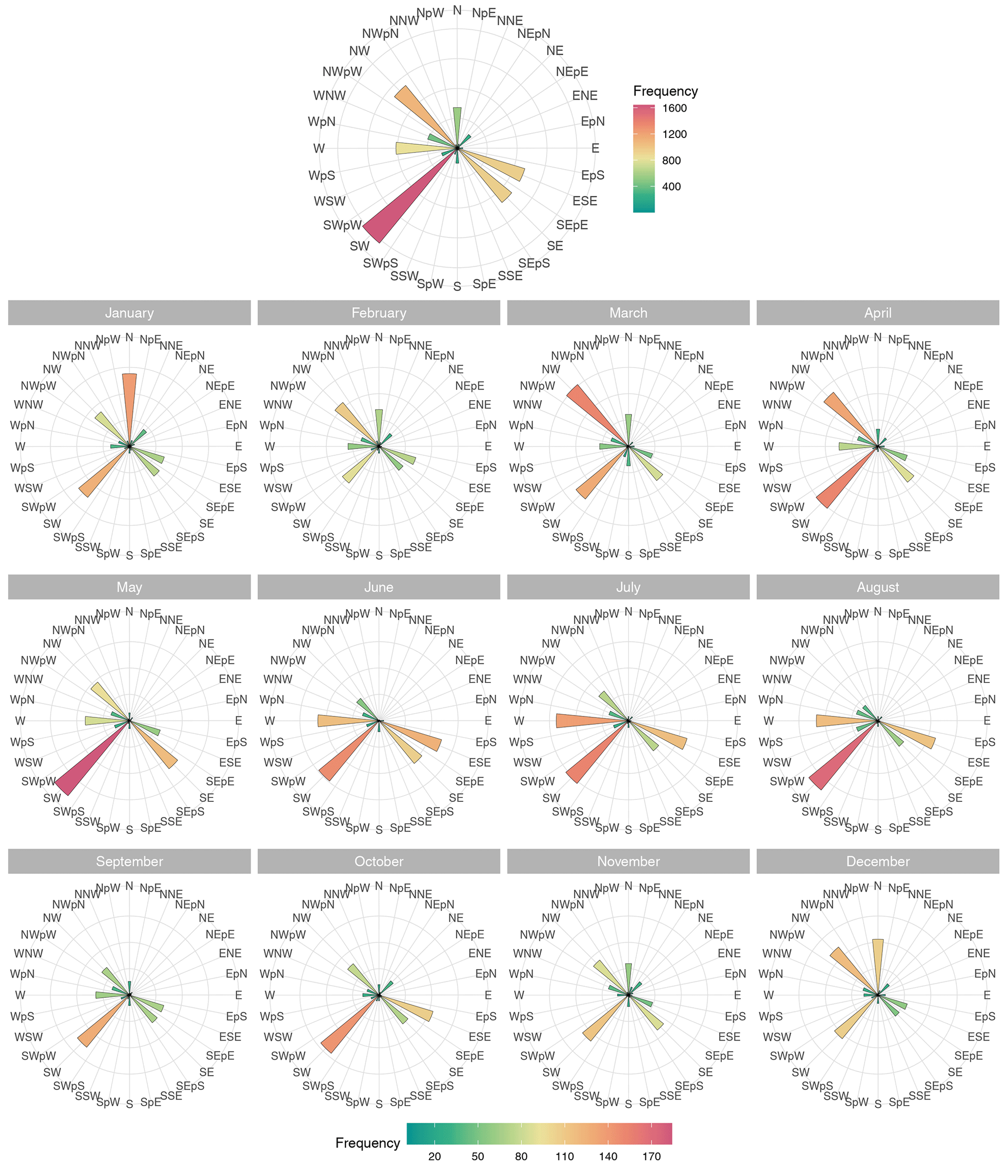
Figure 6Frequency of the wind direction represented in wind compasses for the 1799–1813 period for each month and in total (upper).
Individual subplots represented in Fig. 6 show the frequency of the wind direction represented in wind compasses for the 1799–1813 period for each month and in total (upper subplot). In general, the compasses show five prevalent wind directions (NW, W, SW, SE, and ESE) varying with the seasonal cycle. In winter months (December, January, and February), the predominant wind directions are N, NW, and SW. The SE and ESE wind directions are also relevant but to a lesser extent. In spring months (March, April, and May), the main wind directions are NW, SW, and SE, while in summer months (June, July, and August), the prevalent wind directions are W, SW, and ESE. Finally, in autumn months (September, October, and November), the predominant wind direction is SW, but to a lesser extent other relevant wind directions are NW, SE, and ESE. The predominant wind directions are in accordance with the location of San Fernando, which is closed to the Strait of Gibraltar. In general, the frequency of westerlies is higher than the easterlies, as is expected (Sousa, 1987).
Figure 7 shows the number of observations and the corresponding percentage of the wind force per class (at the top) and the state of the sky (at the bottom) for the period 1799–1813 and 1805–1813, respectively. The terms used to categorize the wind forces are presented with the original Spanish name. These terms could be converted to the Beaufort scale using the CLIWOC dictionary (García-Herrera et al., 2003). There are three predominant wind forces: flojo (Beaufort scale = 3), fresco (Beaufort scale = 6), and fresquito (Beaufort scale = 5). There are also two additional terms with a high number of observations: bonancible (Beaufort scale = 4) and recio (Beaufort scale = 7). Calvo et al. (2008) obtained similar results for Cádiz (about 10 km northwest of San Fernando) for the longer period of 1806–1852. The predominant state of the sky is claro (clear sky). The states of the sky nubes (cloudy) and lluvia (rainy) are also relevant. The term otros in the two figures of Fig. 6 represents those observations with more than one wind force or state of the sky. Nevertheless, this term represents a low number of observations and is not significant.
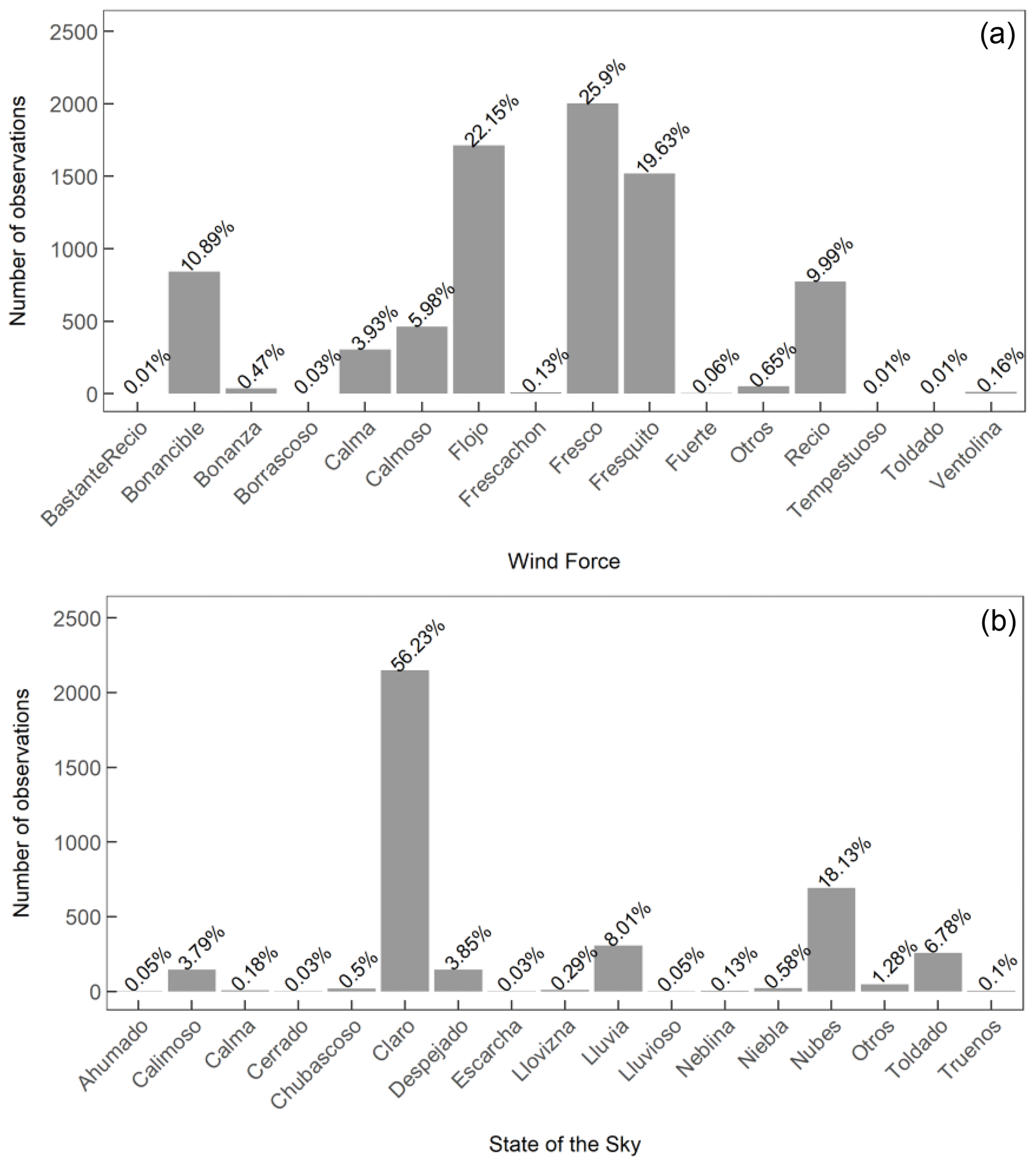
Figure 7(a) Number of observations and the corresponding percentage of the wind force per class for the period 1799–1813 at the top. (b) Number of observations and the percentage of the state of the sky per class for the period 1805–1813.
The accumulated precipitation per month for the period 1805–1813 can be observed in Fig. 8. In the summer months there are no precipitation data. In the metadata there is no information about the absence of observations or the precipitation. For this reason, daily pressure data and periods without rainfall have been plotted together (not shown) to check that there are no drops in pressure values when there are no precipitation data. It seems that the precipitation data are consistent. Monthly values above 100 mm occur almost every autumn–winter, and the highest precipitation values were registered in the month of December in 1812 and October in 1813. Calvo et al. (2008) showed the absolute frequency of precipitation (days per year) of Cádiz for the same period and obtained similar results. The maximum absolute frequency was recorded in 1813, with a frequency of 62 d yr−1. There are no data for the year 1812 (Calvo et al., 2008).
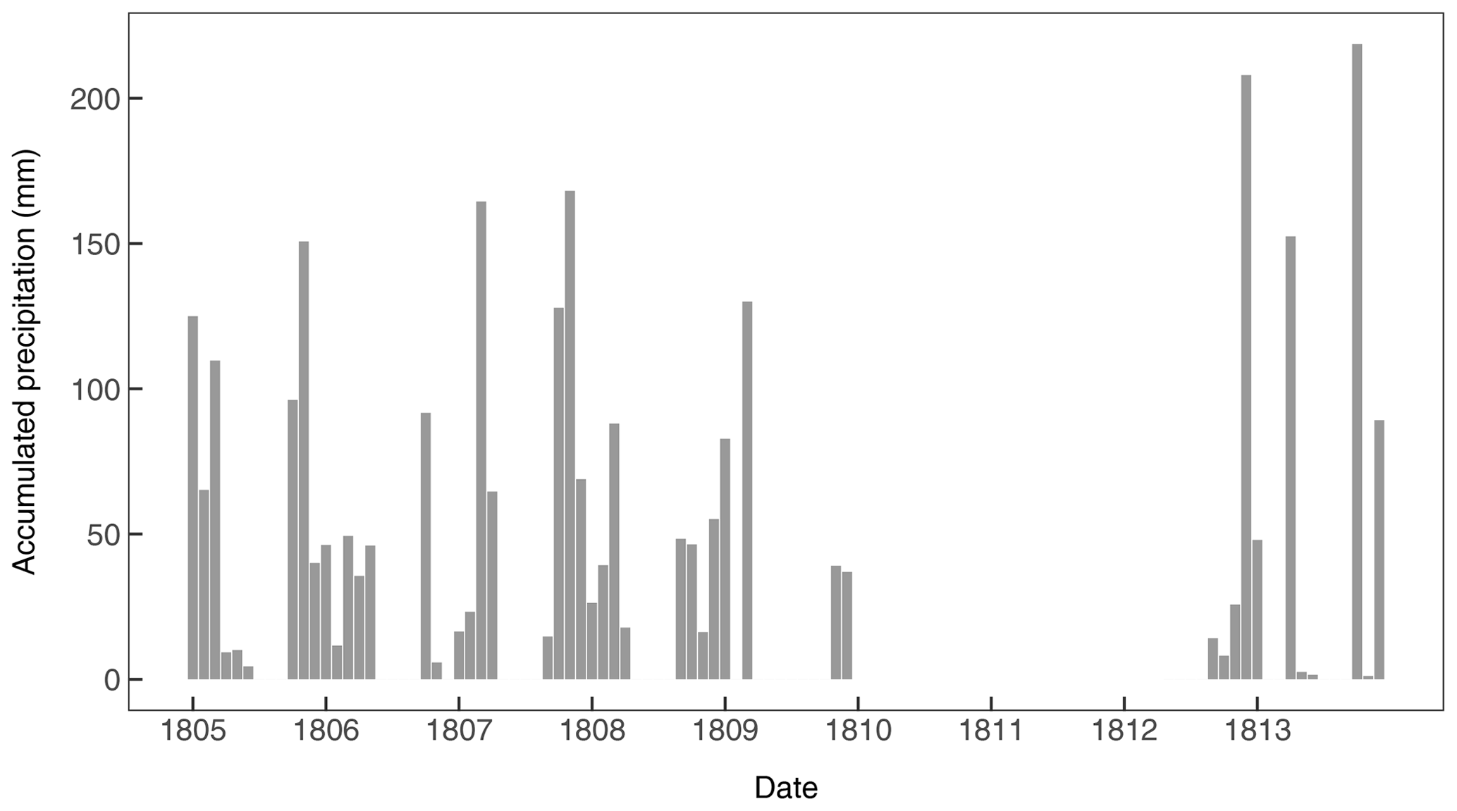
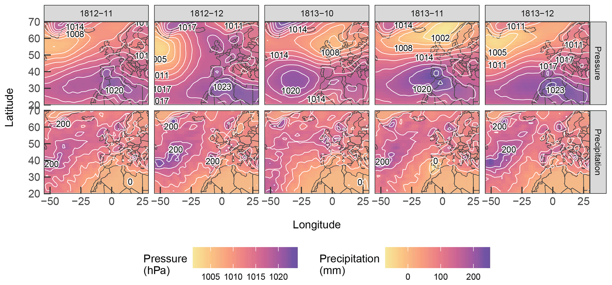
Figure 9Monthly SLP and monthly precipitation anomalies for the months that registered the maximum values of precipitation (see Fig. 7).
The values of sea level pressure (SLP) and the total precipitation (rain and snow) anomalies of the EKF400v2 dataset are represented below for the months of November and December 1812 and the months of October to December 1813 (Fig. 9). The highest precipitation values were recorded in the months of December 1812 and October and December 1813 for the period 1805–1813 (see Fig. 8). In the months of February and March 1813 no precipitation was recorded, but the metadata show several days of rain for February and 1 for March. Therefore, there could be some error in these months, in either the identification of the rainy days or the amount of accumulated precipitation. The precipitation anomalies estimated for the month of December 1812 for southern Spain are around 200 kg m−2 (Fig. 9). For the year 1813, high precipitation values were also estimated for the months of October and December and virtually zero anomaly for the month of November for southern Spain. Pressure values of around 1020 hPa are estimated for the months of November and December 1813 and around 1018 hPa for October 1813. Overall, the large-scale atmospheric dynamics at the monthly scale are in good agreement with the precipitation values represented in Fig. 8 for these months.
The Cádiz–San Fernando region is one of the few places on our planet with a variety of overlapping series of early meteorological data. However, to the best of our knowledge, one of the longest and most interesting series (carried out by the staff of the Royal Observatory of the Spanish Navy) had not been recovered or studied until this work. In total, 45 862 daily meteorological observations of the ROA dataset have been recovered for the period 1799–1813. The dataset is composed of different meteorological variables such as atmospheric pressure, air temperature, precipitation, or state of the sky. After applying a number of quality control steps a small number of values (0.66 % of the data) were detected as suspicious in the digitization process and were corrected. Also, the units have been converted to modern units, and the metadata have been described.
In the comparison between the SF1799-1813 and SF1997-2021 datasets, a significant difference between the pressure values of both series can be observed. Therefore, two adjustments are applied in different periods: for the period 1799–1801 and 1808–1813, a value of 10.3 hPa was added to the pressure observations of SF1799-1813, while for the period 1805–1809 a value of 4.9 hPa was added. Moreover, 0.22 French inches of pressure has been added to the original pressure observations of the SF1799-1813 dataset for the period 1808–1809. The three datasets compared (SF1799-1813, SF1997-2021, and EKF400v2) show a similar behavior for the air temperature data, and there is excellent agreement between air temperature for the SF1799-1813 and SF1997-2021 datasets.
The wind direction frequency analysis shows, when all months of the year are considered, five prevailing wind directions (NW, W, SW, SE, and ESE) for the period 1799–1813. This is in accordance with the location of San Fernando, which is close to the Strait of Gibraltar. In general, the frequency of westerlies is higher than that of the easterlies.
The wind force analysis shows three predominant wind forces (flojo, Beaufort scale = 3; fresco, Beaufort scale = 6; and fresquito, Beaufort scale = 5) for the period 1799–1813. The predominant state of the sky is claro (clear sky) for the period 1805–1813.
The recovered precipitation data show great consistency with respect to the expected climatology: a seasonal cycle with almost no rainfall in the summer months. The years 1812 and 1813 recorded the maximum accumulated precipitation for the period 1805–1813. Unfortunately, observers only recorded precipitation readings when they occurred. Thus, the non-registration of 0 mm of rain entails a certain indeterminacy in these data. In addition, we have found a pair of contradictory data between total monthly precipitation (0 mm) and number of rainy days (other than zero) in the months of February and March 1813.
We would like to see this dataset used for different applications. We are confident that providing free access to this new historical dataset will foster such additional assessments by other researchers.
The SF1799-2013 dataset recovered is publicly available at the Zenodo open data repository at https://doi.org/10.5281/zenodo.7104289 (Bravo-Paredes et al., 2022).
NBP made the data analysis and wrote the first draft of the manuscript. MCG and JMV located the original data and initiated the collaboration. RT, JMV, and MCG wrote and revised the manuscript.
The contact author has declared that none of the authors has any competing interests.
Publisher’s note: Copernicus Publications remains neutral with regard to jurisdictional claims in published maps and institutional affiliations.
This research was supported by the Economy and Infrastructure Counselling of the Junta of Extremadura through project IB20080 and grant GR21080 (co-financed by the European Regional Development Fund). The research of Nieves Bravo-Paredes has been supported by the predoctoral fellowship PRE2018-084897 from Agencia Estatal de Investigación (Ministerio de Ciencia, Innovación y Universidades) of the Spanish Government.
This paper was edited by Chantal Camenisch and reviewed by three anonymous referees.
Alcoforado, M. J., Vaquero, J. M., Trigo, R. M., and Taborda, J. P.: Early Portuguese meteorological measurements (18th century), Clim. Past, 8, 353–371, https://doi.org/10.5194/cp-8-353-2012, 2012.
Auer, I., Böhm, R., Jurkovic, A., Lipa, W., Orlik, A., Potzmann, R., Schöner, W., Ungersböck, M., Matulla, C., Briffa, K., Jones, P., Efthymiadis, D., Brunetti, M., Nanni, T., Maugeri, M., Mercalli, L., Mestre, O., Moisselin, J-M., Begert, M., Müller-Westermeier, G., Kveton, V., Bochnicek, O., Stastny, P., Lapin, M., Szalai, S., Szentimrey, T., Cegnar, T., Dolinar, M., Gajic-Capka, M., Zaninovic, K., Majstorovic, Z., and Nieplova, E.: HISTALP – historical instrumental climatological surface time series of the Greater Alpine Region, Int. J. Climatol., 27, 17–46, https://doi.org/10.1002/joc.1377, 2007.
Barriendos, M., Martín-Vide, J., Peña, J. C., and Rodríguez, R.: Daily Meteorological Observations in Cádiz – San Fernando. Analysis of the Documentary Sources and the Instrumental Data Content (1786–1996), Clim. Change, 53, 151–170, https://doi.org/10.1023/A:1014991430122, 2002.
Bližňák, V., Valente, M. A., and Bethke, J.: Homogenization of time series from Portugal and its former colonies for the period from the late 19th to the early 21st century, Int. J. Climatol, 35, 2400–2418, https://doi.org/10.1002/joc.4151, 2015.
Bravo-Paredes, N., Gallego, M. C., Trigo, R. M., and Vaquero, J. M.: [Data] Earliest meteorological readings in San Fernando (Cádiz, Spain), Zenodo [data set], https://doi.org/10.5281/zenodo.7104289, 2022.
Brönnimann, S., Brugnara, Y., Allan, R. J., Brunet, M., Compo, G. P., Crouthamel, R. I., Jones, P. D., Jourdain, S., Luterbacher, J., Siegmund, P., Valente, M. A., and Wilkinson, C. W.: A roadmap to climate data rescue services, Geosci. Data J., 5, 28–39, https://doi.org/10.1002/gdj3.56, 2018.
Brönnimann, S., Allan, R., Ashcroft, L., Baer, S., Barriendos, M., Brázdil, R., Brugnara, Y., Brunet, M., Brunetti, M., Chimani, B., Cornes, R., Domínguez-Castro, F., Founda, D., Gergis, J., Grab, S., Hannak, L., García-Herrera, R., Huhtamaa, H., Jacobsen, K. S., Jones, P., Jourdain, S., Kiss, A., Lin, K. E., Lorrey, A., Lundstad, E., Luterbacher, J., Moberg, A., Mauelshagen, F., Maugeri, M., Maughan, N., Neukom, R., Nicholson, S., Noone, S., Nordli, Ø., Ólafsdóttir, K. B., Pearce, P. R., Pfister, L., Pribyl, K., Przybylak, R., Pudmenzky, C., Rasol, D., Reichenbach, D., Řezníčková, L., Rodrigo, F. S., Rohde, R., Rohr, C., Skrynyk, O., Slonosky, V., Thorne, P., Valente, M. A., Vaquero, J. M., Westcottt, N. E., Williamson, F., and Wyszyński, P.: Unlocking pre-1850 instrumental meteorological records: A global inventory, B. Am. Meteorol. Soc. 100, ES389–ES413, https://doi.org/10.1175/BAMS-D-19-0040.1, 2019.
Brugnara, Y., Pfister, L., Villiger, L., Rohr, C., Isotta, F. A., and Brönnimann, S.: Early instrumental meteorological observations in Switzerland: 1708–1873, Earth Syst. Sci. Data, 12, 1179–1190, https://doi.org/10.5194/essd-12-1179-2020, 2020.
Calvo, N., Gallego, D., García-Herrera, R., Gullón, A., Portela, M. J., Prieto, M. R., and Ribera, P.: El clima de Cádiz en la primera mitad del silgo XIX según los parte de la Vigía, edited by: García-Herrera, R., Servicio de Publicaciones de la Fundación Unicaja, Málaga, Spain, ISBN 978-84-95979-69-8, 2008.
Camuffo, D. and Jones, P.: Improved Understanding of Past Climatic Variability from Early Daily European Instrumental Sources, in: Improved Understanding of Past Climatic Variability from Early Daily European Instrumental Sources, vol. 53, edited by: Camuffo, D. and Jones, P., Springer, Dordrecht, 1–4, https://doi.org/10.1007/978-94-010-0371-1_1, 2002.
Cornes, R. C., Jones, P. D., Briffa, K. R., and Osborn, T. J.: A daily series of mean sea-level pressure for Paris, 1670–2007, Int. J. Climatol., 32, 1135–1150, https://doi.org/10.1002/joc.2349, 2012.
Domínguez-Castro, F., Vaquero, J. M., Rodrigo, F. S., Farrona, A. M. M., Gallego, M. C., García-Herrera, R., Barriendos, M., and Sanchez-Lorenzo, A.: Early Spanish meteorological records (1780–1850), Int. J. Climatol., 34, 593–603, https://doi.org/10.1002/joc.3709, 2014.
Domínguez-Castro, F., Vaquero, J. M., Gallego, M. C., Farrona, A. M. M., Antuña-Marrero, J. C., Cevallos, E. E., García-Herrera, R., de la Guía, C., Mejía, R. D., Naranjo, J. M., Prieto, M. R., Ramos Guadalupe, L. E., Seiner, L., Trigo, R. M., and Villacís, M.: Early meteorological records from Latin- America and the Caribbean during the 18th and 19th centuries, Sci. Data, 4, 1–10, https://doi.org/10.1038/sdata.2017.169, 2017.
Dunnington, D.: Ggspatial: spatial data framework for ggplot2, R package version 1.1.1, https://CRAN.R-project.org/package=ggspatial (Last access: 4 July 2023), 2020.
Farrona, A. M. M., Trigo, R. M., Gallego, M. C., and Vaquero, J. M.: The meteorological observations of Bento Sanches Dorta, Rio de Janeiro, Brazil: 1781–1788, Clim. Change, 115, 579–595, https://doi.org/10.1007/s10584-012-0467-8, 2012.
Gallego, D., García-Herrera, R., Calvo, N., and Ribera, P.: A new meteorological record for Cádiz (Spain) 1806–1852: Implications for climatic reconstructions. J. Geophys. Res.-Atmos., 112, D12108, https://doi.org/10.1029/2007JD008517, 2007.
García-Herrera, R., Prieto, L., Gallego, D., Hernández, E., Gimeno, L., Können, G., Koek, F., Wheeler, D., Wilkinson, C., Prieto, M., Báez, C., and Woodruff, S: CLIWOC multilingual meteorological dictionary, https://epic.awi.de/id/eprint/17064/ (last access: 4 July 2023), 2003.
Jones, P. D., Davies, T. D., Lister, D. H., Slonosky, V., Jónsson, T., Bärring, L., Jönsson, P., Maheras, P., Kolyva-Machera, F., Barriendos, M., Martin-Vide, J., Rodriguez, R., Alcoforado, M. J., Wanner, H., Pfister, C., Luterbacher, J., Rickli, R., Schuepbach, E., Kaas, E., Schmith, T., Jacobeip, J., and Beck, C.: Monthly mean pressure reconstructions for Europe for the 1780–1995 period, Int. J. Climatol., 19, 347–364, https://doi.org/10.1002/(SICI)1097-0088(19990330)19:4<347::AID-JOC363>3.0.CO;2-S, 1999.
Können, G. P. and Brandsma, T.: Instrumental pressure observations from the end of the 17th century: Leiden (The Netherlands), Int. J. Climatol., 25, 1139–1145, https://doi.org/10.1002/joc.1192, 2005.
Lafuente, A. and Sellés, M.: El Observatorio de Cádiz (1753–1831), Ministerio de Defensa, Instituto de Historia y Cultura Naval, Madrid, ISBN 84-505-7563-X, 1988.
Luterbacher, J., Rickli, R., Tinguely, C., Xoplaki, E., Schüpbach, E., Dietrich, D., Hüsler, J., Ambühl, M., Pfister, C., Beeli, P., Dietrich, U., Dannecker, A., Davies, T. D., Jones, P. D., Slonosky, V., Ogilvie, A. E. J., Maheras, P., Kolyva-Machera, F., Martin-Vide, J., Barriendos, M., Alcoforado, M. J., Nunes, M. F., Jónsson, T., Glaser, R., Jacobeit, J., Beck, C., Philipp, A., Beyer, U., Kaas, E., Schmith, T., Bärring, L., Jönsson, P., Rácz, L., and Wanner, H.: Monthly mean pressure reconstruction for the Late Maunder Minimum Period (AD 1675–1715), Int. J. Climatol., 20, 1049–1066, https://doi.org/10.1002/1097-0088(200008)20:10<1049::AID-JOC521>3.0.CO;2-6, 2000.
Morozova, A. L. and Valente, M. A.: Homogenization of Portuguese long-term temperature data series: Lisbon, Coimbra and Porto, Earth Syst. Sci. Data, 4, 187–213, https://doi.org/10.5194/essd-4-187-2012, 2012.
Pfister, L., Hupfer, F., Brugnara, Y., Munz, L., Villiger, L., Meyer, L., Schwander, M., Isotta, F. A., Rohr, C., and Brönnimann, S.: Early instrumental meteorological measurements in Switzerland, Clim. Past, 15, 1345–1361, https://doi.org/10.5194/cp-15-1345-2019, 2019.
Picas, J., Grab, S., and Allan, R.: A 19th century daily surface pressure series for the Southwestern Cape region of South Africa: 1834–1899, Int. J. Climatol., 39, 1404–1414, https://doi.org/10.1002/joc.5890, 2019.
Pujazón, C.: Resumen de las observaciones pluviométricas efectuadas en los años 1805 a 1899, Instituto y Observatorio de Marina, San Fernando, Cádiz, 1899.
Rodrigo, F. S.: Completing the early instrumental weather record from Cádiz (Southern Spain): New data from 1799 to 1803, Clim. Change, 111, 697–704, https://doi.org/10.1007/s10584-011-0174-x, 2012.
Rodrigo, F. S.: Early meteorological data in southern Spain during the Dalton Minimum, Int. J. Climatol., 39, 3593–3607, https://doi.org/10.1002/joc.6041, 2019.
Slonosky, V.: The Meteorological Observations of Jean-François Gaultier, Quebec, Canada: 1742–56, J. Climate, 16, 2232–2247, https://doi.org/10.1175/1520-0442(2003)16<2232:TMOOJG>2.0.CO;2, 2003.
Slonosky, V. C., Jones, P. D., and Davies, T. D.: Instrumental pressure observations and atmospheric circulation from the 17th and 18th centuries: London and Paris, Int. J. Climatol., 21, 285–298, https://doi.org/10.1002/joc.611, 2001.
Sousa, R.: Notas para una Climatología de Cádiz, Ministerio de Transportes, Turismo y Comunicaciones, Madrid, ISBN 84-505-6878-1, 1987.
Valler, V., Franke, J., Brugnara, Y., and Brönnimann, S.: An updated global atmospheric paleo-reanalysis covering the last 400 years, Geosci. Data J., 1–19, https://doi.org/10.1002/gdj3.121, 2021.
Vaquero, J. M., Bravo-Paredes, N., Obregón, M. A., Carrasco, V. M. S., Valente, M. A., Trigo, R. M., Domínguez-Castro, F., Montero-Martín, J., Vaquero-Martínez, J., Antón, M., García, J. A., and Gallego, M. C.: Recovery of early meteorological records from Extremadura region (SW Iberia): The “CliPastExtrem” (v1.0) database, Geosci. Data J., 9, 1–14, https://doi.org/10.1002/gdj3.131, 2022.
Wheeler, D.: Early instrumental weather data from Cadiz: A study of late eighteenth and early nineteenth century records, Int. J. Climatol., 15, 801–810, https://doi.org/10.1002/joc.3370150707, 1995.
WMO: Guide to meteorological instruments and methods of observation; WMO-No. 8: Measurement of Meteorological Variables, 525–552, ISBN 978-92-63-100085, 2018.
Zaiki, M., Kimura, K., and Mikami, T.: A statistical estimate of daily mean temperature derived from a limited number of daily observations, Geophys. Res. Lett., 29, 39.1–39.4, https://doi.org/10.1029/2001GL014378, 2002.
Zaiki, M., Können, G. P., Tsukahara, T., Jones, P. D., Mikami, T., and Matsumoto, K.: Recovery of nineteenth-century Tokyo/Osaka meteorological data in Japan, Int. J. Climatol., 26, 399–423, https://doi.org/10.1002/joc.1253, 2006.