Amplified surface warming in the south-west Pacific during the mid-Pliocene (3.3–3.0 Ma) and future implications

Based on Nationally Determined Contributions concurrent with Shared Socioeconomic Pathways (SSPs) 2-4.5, the IPCC predicts global warming of 2.1–3.5 ^∘C (very likely range 10–90th percentile) by 2100 CE. However, global average temperature is a poor indicator of regional warming and global climate models (GCMs) require validation with instrumental or proxy data from geological archives to assess their ability to simulate regional ocean and atmospheric circulation, and thus, to evaluate their performance for regional climate projections. The south-west Pacific is a region that performs poorly when GCMs are evaluated against instrumental observations. The New Zealand Earth System Model (NZESM) was developed from the United Kingdom Earth System Model (UKESM) to better understand south-west Pacific response to global change, by including a nested ocean grid in the south-west Pacific with 80 % greater horizontal resolution than the global-scale host.

Here, we reconstruct regional south-west Pacific sea-surface temperatures (SSTs) for the mid-Pliocene warm period (mPWP; 3.3–3.0 Ma), which has been widely considered a past analogue with an equilibrium surface temperature response of +3 ^∘C to an atmospheric CO₂ concentration of ∼350–400 ppm, in order to assess the warming distribution in the south-west Pacific. This study presents proxy SSTs from seven deep sea sediment cores distributed across the south-west Pacific. Our reconstructed SSTs are derived from molecular biomarkers preserved in the sediment – alkenones (i.e. U${}_{\mathrm{37}}^{\mathrm{K}{}^{\prime }}$ index) and isoprenoid glycerol dialkyl glycerol tetraethers (i.e. TEX₈₆ index) – and are compared with SSTs reconstructed from the Last Interglacial (125 ka), Pliocene Model Intercomparison Project (PlioMIP) outputs and transient climate model projections (NZESM and UKESM) of low- to high-range SSPs for 2090–2099 CE.

Mean interglacial equilibrium SSTs during the mPWP for the south-west Pacific sites were on average 4.2 ^∘C (1.8–6.1 ^∘C likely range) above pre-industrial temperatures and show good agreement with model outputs from NZESM and UKESM under mid-range SSP 2–4.6 conditions. These results highlight that not only is the mPWP an appropriate analogue when considering future temperature change in the centuries to come, but they also demonstrate that the south-west Pacific region will experience warming that exceeds that of the global mean if atmospheric CO₂ remains above 350 ppm.

1 Introduction

The latest IPCC climate projections to 2100 CE project average global surface warming of 1.4–4.4 ^∘C depending on the emissions pathway (IPCC, 2022). While limiting global warming to 1.5 ^∘C urgently requires policies and actions to bring about steep emission reductions this decade, global warming could be stabilised at 2.0 ^∘C, if the latest Nationally Determined Contributions are achieved (Meinshausen et al., 2022). Despite stabilising at 2.0 ^∘C, heat taken up by the ocean and the polar ice sheets would ensure that the global sea level would continue to rise for centuries to come (IPCC, 2022). Warming above 2.0 ^∘C may trigger rapid unstoppable collapse of the marine-based sectors of the Antarctic Ice Sheets, with one model for a high-emissions scenario suggesting global mean sea-level rise of up to 2 m by 2100 CE and 13 m by 2300 CE (DeConto et al., 2021; IPCC, 2022). Notwithstanding the high-end scenarios, a stability threshold for Antarctic ice shelves is crossed above +2.0 ^∘C that commits the planet to multi-metre, multi-century sea-level rise (DeConto and Pollard, 2016; Golledge et al., 2019; Lowry et al., 2021). Additionally, the regional expression of global warming can differ significantly from global averages, as is evident from most land regions currently recording warming which exceeds the global average (Hoegh-Guldberg et al., 2018; Sutton and Bowen, 2018; Doblas-Reyes et al., 2021). Regionally focussed climate models are necessary for island nations with oceanic influence and dramatic topography such as New Zealand, since these parameters are unresolvable at the spatial resolutions used by climate models with a low, uniform resolution (Doblas-Reyes et al., 2021).

Here, we consider the regional climate of the south-west Pacific and Southern Ocean, which is often misrepresented due to the coarse resolution and biases introduced in global climate models (GCMs; Behrens et al., 2020, 2022; Williams et al., 2023). Steep regional gradients in sea-surface temperature (SST), salinity and nutrients characterise water masses spanning the south-west Pacific and New Zealand continent (Zealandia – Te Riu-a-Māui; Ridgway, 2007; Chiswell et al., 2015; Chiswell, 2021), which represents a key location for southward heat transport balanced by northward flow of deep western boundary currents (Carter et al., 2004). Subtropical waters are transported southward through surface eddies and the East Australian Current (EAC) and Tasman Front (Fig. 1; Behrens et al., 2019). Zealandia is situated at the confluence of relatively cool, fresh, nutrient-rich Subantarctic Water and warm, salty, nutrient-poor Subtropical Water, defining the Subtropical Front (e.g. Chiswell et al., 2015; Fig. 1). The New Zealand Earth System Model (NZESM) was developed from its parent model, the United Kingdom Earth System Model (UKESM), to address the need for higher spatial resolution in models across Zealandia (Williams et al., 2016). An increased horizontal grid resolution from 1 to 0.2^∘ better simulates boundary currents and surface eddies and results in an increased meridional heat transport from the Equator to higher southern latitudes (Behrens et al., 2019) and is in better agreement with historical observations compared to the UKESM (Behrens et al., 2020).

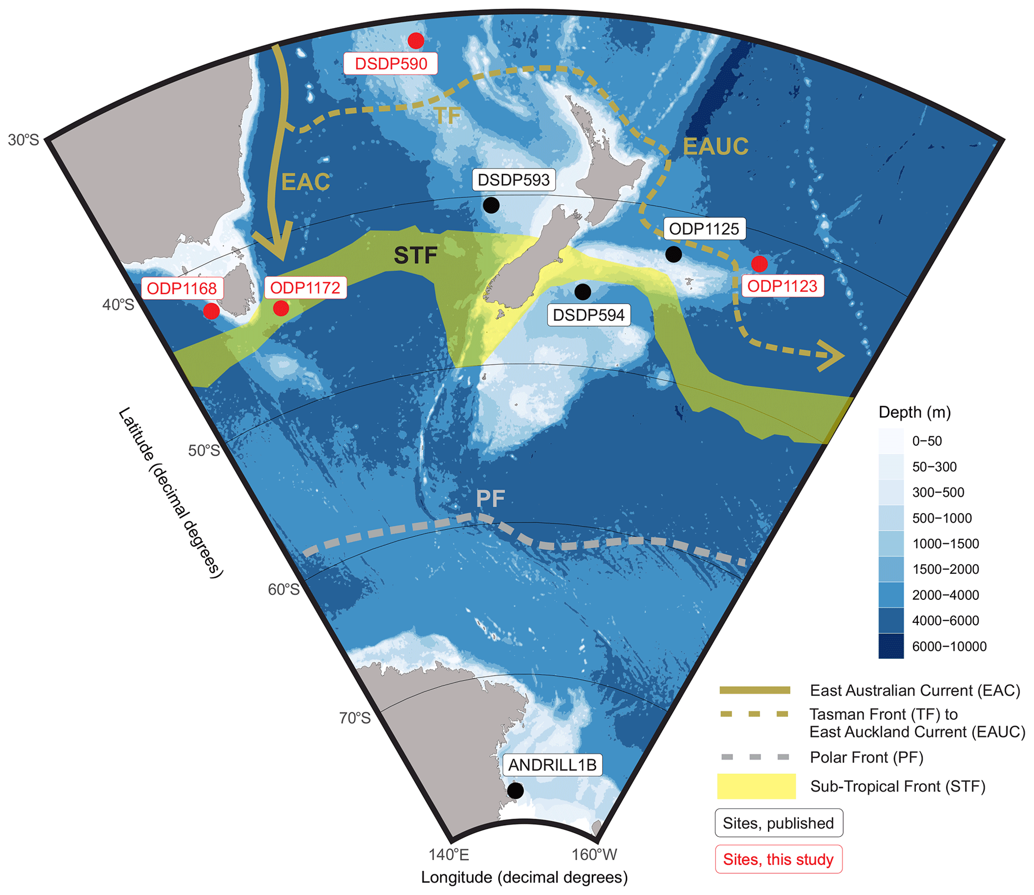
Figure 1 Location map for sites used in the south-west Pacific SST reconstruction (north: top of page). Sites in black have been previously published and sites in red were analysed in this study. Present-day surface ocean circulation and fronts referenced in text are displayed. Note ODP 806 (0.3^∘ N 159.4^∘ E) is not displayed in this projection. Bathymetry is plotted using “ggOceanMaps” (Vihtakari, 2022) and bathymetry data are sourced from Amante and Eakins (2022).

Past climate data allow the reconstruction of the equilibrium climate states in response to both fast and slow Earth system feedback involving the cryosphere, ocean and atmospheric circulation and the carbon cycle. Data from these geological archives for times representing higher-than-present CO₂ worlds have been widely used in Climate Model Intercomparison Projects (CMIPs) to assess the performance of transient GCMs run to equilibrium (e.g. Haywood et al., 2019; Masson-Delmotte et al., 2013). While most CMIPs reconcile global mean temperatures, they poorly reconcile regional climatic patterns such as polar amplification (Naish and Zwartz, 2012; Haywood et al., 2019; Masson-Delmotte et al., 2013; Fischer et al., 2018). This is in part due to the incomplete spatial coverage of the geological data, accuracy and quality of the data, the resolution of GCM grids and their treatment of mid- to high-latitude polar processes. Equilibrium climate sensitivity (ECS; model warming associated with a doubling of CO₂ once the energy balance has reached equilibrium) is one important measure of how models perform on longer timescales. An increase in ECS from the CMIP Phase 5 to the CMIP Phase 6 ensemble has been linked to shortwave cloud feedback, which has significant impact over the Southern Ocean (Zelinka et al., 2020; Zhu et al., 2021). Higher ECS is more consistent with estimates of warmer-than-present palaeoclimate sensitivity (Forster et al., 2021).

We assess the magnitude and distribution of warming for the south-west Pacific for various emissions scenarios and discuss the differences between the GCMs and palaeoclimate reconstructions and consider the implications for interpreting projections of future warming in the SW Pacific.

1.1 Palaeoclimate analogues

1.1.1 Mid-Pliocene warm period (3.3–3.0 Ma)

Global temperatures (+2 to 3 ^∘C) last experienced during the Mid-Pliocene warm period (mPWP; 3.3–3.0 Ma) may be reached by 2100 CE if emissions are abated in line with the Shared Socioeconomic Pathways (SSPs) 2–4.5 scenario, which is the pathway aligned to current policy (not the aspirational 1.5 ^∘C Paris target; Burke et al., 2018). The mPWP spans a 300 kyr period when atmospheric CO₂ was comparable to the present day (mean 390 ppm; Chalk et al., 2017; De La Vega et al., 2020). During this period interglacial global temperatures were 2–3 ^∘C warmer (Dowsett et al., 2013; Masson-Delmotte et al., 2013), and the amplitude of glacial–interglacial sea-level change was likely between 6 and 17 m (16th–84th percentile; Grant et al., 2019; Grant and Naish, 2021). Such a rise in global sea level implies melting of the Greenland Ice Sheet (Koenig et al., 2015; Batchelor et al., 2019), West Antarctic Ice Sheet (Naish et al., 2009; McKay et al., 2012) and parts of the marine-based East Antarctic Ice Sheet (Cook et al., 2013; Patterson et al., 2014; Bertram et al., 2018). Therefore, the interglacial periods of mPWP are considered to be the most accessible and suitable past analogue, or window, into the future equilibrium response of the Earth system to warming in line with SSP2–4.5 (Naish and Zwartz, 2012; Dowsett et al., 2013; Haywood et al., 2019).

The mPWP has been the focus of several major international research initiatives. The Pliocene Research, Interpretation and Synoptic Mapping (PRISM) project (Dowsett et al., 2013, 2016) undertook a global compilation of palaeoclimate data, primarily surface temperature reconstructions. The Pliocene Model Intercomparison Project (PlioMIP) presents a multi-model ensemble with various ECS run for mPWP conditions (Haywood et al., 2011; 2016, 2020). The recent IPCC summary of ECS ranges from median values of 2.5 to 3.7 ^∘C (Forster et al., 2021). This ECS summary does not include model-based estimates but does include emergent constraints (Hargreaves and Annan, 2016; Renoult et al., 2020) utilising PlioMIP (Haywood et al., 2020) and proxy temperature and CO₂ reconstructions (Martínez-Botí et al., 2015; Sherwood et al., 2020).

Marine isotope stage (MIS) KM5c (3.2 Ma) interglacial became a focus for reconstructing warming within mPWP as insolation values and the orbital configuration were most similar to the Holocene interglacial (Haywood et al., 2020; McClymont et al., 2020). While, based on less data points, this approach has better agreement between models and observations and revealed a higher ECS of 2.6–4.8 ^∘C for conditions of MIS KM5c from the PlioMIP Phase 2 ensemble (PlioMIP2; Haywood et al., 2020), a recent review of SSTs in the mPWP for MIS KM5c by the PlioVAR working group (Pliocene climate variability on glacial–interglacial timescales; McClymont et al., 2020) used alkenones to reconstruct an average global SST warming of 3.2–3.4 ^∘C above pre-industrial SST. This is slightly warmer than PlioMIP2 simulations, where global surface air temperature over oceans were ∼2.8 ^∘C above pre-industrial temperatures. However, differences are suggested to be due to regional ocean circulation and proxy signals (McClymont et al., 2020).

While interglacial minima and glacial maxima in the benthic δ¹⁸O stack (MISs) have been the primary means of reconstructing the timing and magnitude of global sea-level variations over the last 5 Myr (Lisiecki and Raymo, 2005), for some time intervals (i.e. mPWP) global sea level is known to fluctuate at a higher frequency than can be assessed in the benthic δ¹⁸O stack (Grant et al., 2019). This is also the case for other proxies with variable sampling resolution such as SSTs that have not been tuned to the δ¹⁸O stack (e.g. Herbert et al., 2010; Fig. 2). The reliance on orbitally tuned timescales in deep ocean palaeoclimate records has potentially led to misinterpretation of the timing, frequency and amplitude of glacial–interglacial climate change. This is particularly the case in the Pliocene and Early Pleistocene, where there are less globally distributed δ¹⁸O records and many are of coarse sampling resolution (Lisiecki and Raymo, 2005). In a number of studies (Lisiecki and Raymo, 2005; Miller et al., 2012; Grant et al., 2019), average glacial climate conditions (global surface temperature and sea level) during the mPWP have been considered similar to those of the Holocene.

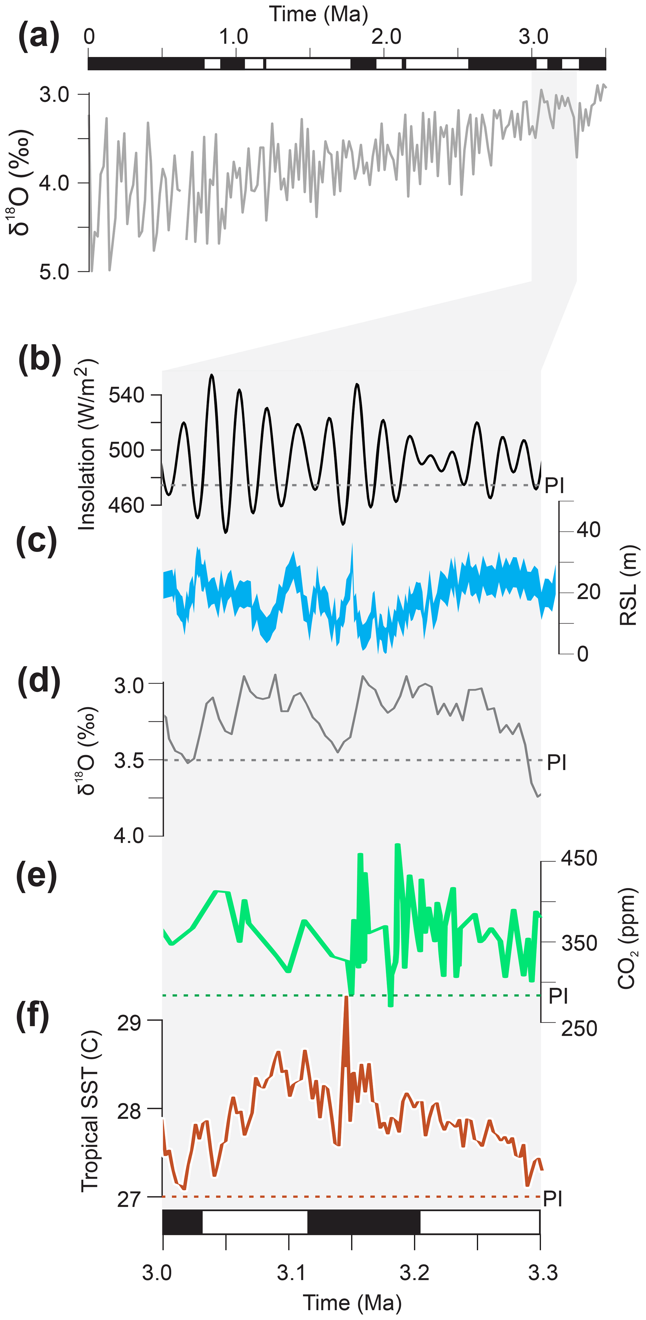
Figure 2 Mid-Pliocene warm period (mPWP) climate context showing reconstructions of (a) a combined signal of global sea level and ocean temperature from deep sea benthic δ¹⁸O data (Lisiecki and Raymo, 2005) spanning mPWP to the present; (b) daily insolation at 65^∘ N (21 June: Laskar et al., 2004); (c) global relative sea-level change from PlioSeaNZ (Pliocene sea level record), Whanganui Basin, New Zealand (Grant et al., 2019); (d) a combined signal of global sea level and ocean temperature from deep sea benthic δ¹⁸O data mPWP (3.3–3.0 Ma) of Lisiecki and Raymo (2005); (e) atmospheric CO₂ from δ¹¹B-pH proxy (De La Vega et al., 2020) and (f) tropical SSTs from alkenone palaeothermometry (Herbert et al., 2010). Pre-industrial estimates are also shown.

1.1.2 Last Interglacial (125 ka)

Finally, we briefly compare these results to the Last Interglacial MIS 5e (∼125 ka) as many of the sites investigated here were also used by Cortese et al. (2013) in a proxy SST study. Peak interglacial SSTs were reconstructed from core-top planktonic foraminiferal assemblages, calibrated to modern SSTs and then applied to palaeo-assemblages (Cortese et al., 2013). The south-west Pacific study presented warming focussed in Tasmania and western New Zealand and proposed a strengthened EAC bathing Tasmania with warmer water (Cortese et al., 2013). MIS 5e represents a lower global average temperature increase of 1–2 ^∘C above pre-industrial temperature in response to changing orbital configurations on radiative forcing (rather than CO₂), associated with 6–9 m of sea-level rise, which together with the mPWP analogue discussed above implies extreme sensitivity of the polar ice sheets to relatively small changes in global mean surface temperature (Dutton et al., 2015).

1.2 Future scenarios

Here we display model results of future projections from NZESM and UKESM. These are previously published and thus introduced here, while the comparisons to data presented in this study are discussed in detail in Sect. 3.

The NZESM (Williams et al., 2016, Behrens et al., 2020) is based on the UKESM (Sellar et al., 2019; Senior et al., 2020), a CMIP6 Earth system model (ESM) containing a dynamic atmosphere, ocean, prognostic sea ice, complex atmospheric chemistry and ocean biogeochemistry. Via a two-way nesting scheme, ocean physical parameters were dynamically downscaled from 1 to 0.2^∘ in the NZESM to better simulate boundary currents and mesoscale variability, instrumental for southward heat transport (Behrens et al., 2019). This nesting improves the steady state simulated sea-surface properties (Behrens et al., 2020, 2022). With the exception of a solar cycle dependence of the ozone photolysis scheme included in the NZESM (Dennison et al., 2019), the atmospheric physics is identical to the UKESM in all other respects. Globally averaged SSTs are marginally warmer than the UKESM in all pathways up to 2100 CE, but that difference is reduced as the magnitude of warming increases under higher-emission scenarios (Fig. 3). Indeed, for 2090–2099 CE in SSP3–7.0, the mean difference between the two models is essentially zero for higher greenhouse gas levels. This global signal is dominated by the Southern Hemisphere warming induced by increased southward heat transport from the tropics in the NZESM.

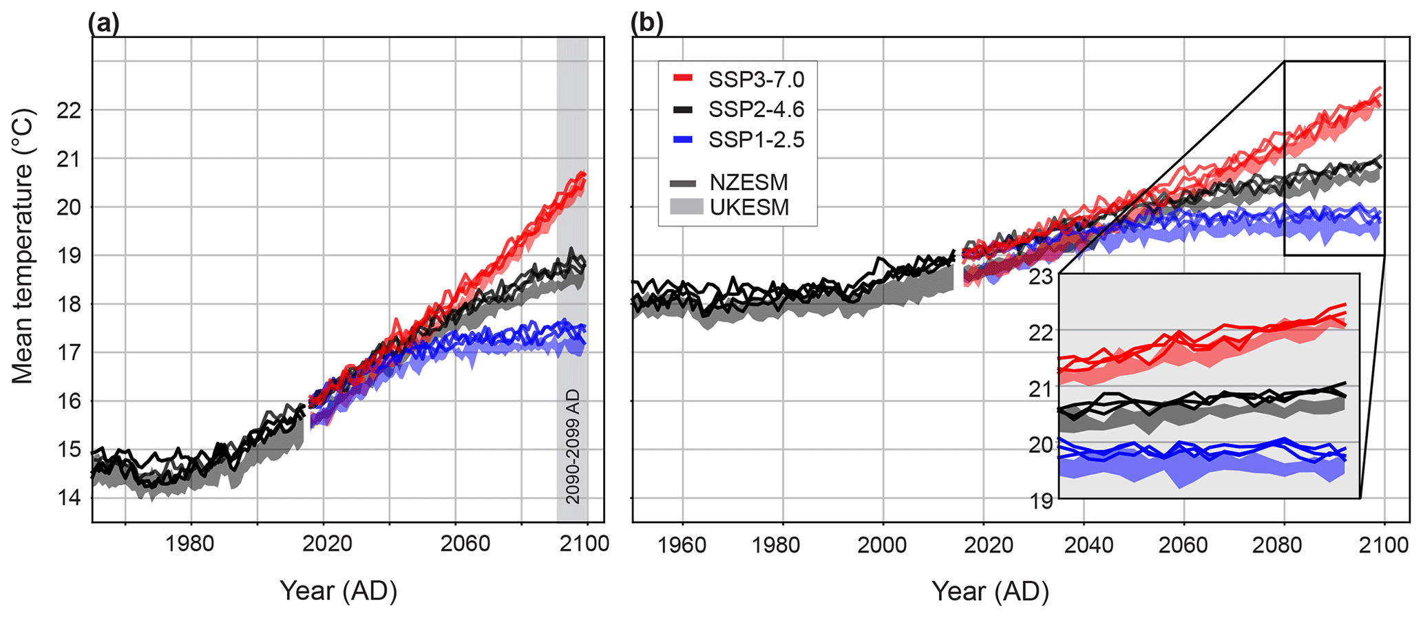
Figure 3 Mean Surface Air Temperature from NZESM and UKESM simulations of low- to high-range emission Shared Socioeconomic Pathways (SSPs) for (a) the global region and (b) the area covered by the high-resolution ocean grid of NZESM. Results generated from the UKESM (Sellar et al., 2019) and NZESM (Williams et al., 2016; Behrens et al., 2022) projections used in this study are extracted for all SSPs for 2090–2099 CE.

The latest climate projections are grouped according to primary Shared Socioeconomic Pathways (SSPs; Lee et al., 2021) forced by various greenhouse gas emissions and other radiative forcings and simulated by the CMIP6 (Eyring et al., 2016). These pathways are differentiated by degrees of very likely warming by 2100 CE, i.e. 1.3–2.4 ^∘C (SSP1 – sustainability), 2.1–3.5 ^∘C (SSP2 – middle of the road) and 2.5–4.6 ^∘C (SSP3 – regional rivalry; Chen et al., 2021; O'Neill et al., 2016). NZESM and UKESM were both run for SSP1–2.6, SSP2–4.5 and SSP3–7.0, broadly correspond to low, medium and high emissions scenarios and were run out to 100 CE. While UKESM was run for other SSPs, NZESM was not, so we have restricted comparison to these scenarios.

The UKESM (a CMIP ensemble member) and NZESM have an ECS of 5.4 ^∘C (Sellar et al., 2019), which is higher than the likely range (high confidence) for ECS as 2.5–4 ^∘ C (Zelinka et al., 2020). This is most clearly seen in the degree of global warming (Fig. 3a) compared to the regional warming of the high-resolution NZESM ocean-grid area (Fig. 3b). Climate scenarios by the 2090–2099 CE period generated warming of (i) ∼3 ^∘C globally and ∼2 ^∘C regionally for SSP1–2.6, (ii) 4 ^∘C globally and 3 ^∘C regionally for SSP2–4.5 and (iii) 6 ^∘C globally and 4.5 ^∘C regionally for SSP3–7.0 (Fig. 3). This differs (by close to half) from mean global warming from the CMIP6 model ensemble of ∼1.8, 2.7 and 3.6 ^∘C for SSP1–2.6, 2–4.5 and 3–7.0 respectively by 2100 CE (IPCC, 2022). Annual mean SSTs were extracted for all sites and are reported here. Sites in the tropics (ODP 806) and Southern Ocean (Antarctic Drilling Project, ANDRILL) were excluded as they are outside of the NZESM high-resolution ocean-grid region.

As a reference or pre-industrial control, the results generated from the Hadley Centre Global Sea Ice and Sea Surface Temperature (HadISST) model were used for 1870–1879 CE (NCAR, 2022; Rayner et al., 2003). Best practise of model assessment is to present anomalies with reference to pre-industrial runs from the same model. As a pre-industrial run is unavailable for the NZESM, we have used the single reference of HadISST for all model and proxy anomaly assessments. HadISST was selected as it is the most complete reanalysis product nearest to pre-industrial conditions.

2 Methods

To enable comparison of past SSTs with future projections, we assess the full duration and glacial-to-interglacial amplitude of the mPWP, for sites across the south-west Pacific region. In this approach, glacial and interglacial modal means are determined statistically to ensure the pattern and magnitude of warming is more representative of mPWP interglacial climate conditions as opposed to the single peak interglacial conditions that have been the focus of previous climate reconstructions (Dowsett et al., 2016; Haywood et al., 2020; McClymont et al., 2020). We have applied the U${}_{\mathrm{37}}^{\mathrm{K}{}^{\prime }}$ index (unsaturated ketone index; Prahl and Wakeham, 1987) to reconstruct SSTs at four new sites (DSDP 590, ODP 1123, ODP 1168 and ODP 1172) which complement three sites with previously published U${}_{\mathrm{37}}^{\mathrm{K}{}^{\prime }}$-derived SSTs (DSDP 593: McClymont et al., 2016; DSDP 594 and ODP 1125: Caballero-Gill et al., 2019). We have also applied TEX₈₆ (TetraEther indeX of tetraether consisting of 86 carbon atoms) most commonly correlated with SST or shallow subsurface (50–200 m) temperatures (Tierney and Tingley, 2015) at two of the sites (DSDP 590 and ODP 1172). Two additional sites, ODP 806 (Eastern Equatorial Pacific: Medina-Elizalde and Lea, 2010) and ANDRILL (Ross Sea, Antarctica; McKay et al., 2012) are located outside of the south-west Pacific and provide a meridional climate context.

We extract site-specific simulated SSTs from PlioMIP and future UKESM and NZESM to compare the reconstructed pattern of warming in the south-west Pacific during the mPWP.

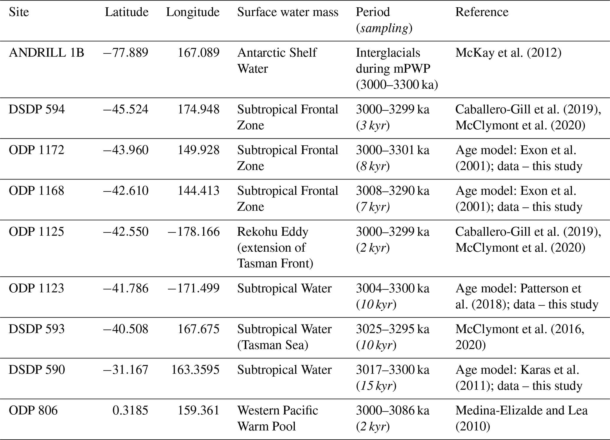
Table 1 Mid-Pliocene warm period (mPWP) site identification and location with associated surface water mass, sampling period and resolution (italicised in parenthesis) and source references for previously published data or age models used in association with new analyses.

2.1 Mid-Pliocene warm period records

Sea-surface temperature records from nine sites are presented in this study, including published SST data from five sites and new SST data from four sites to improve the geographical resolution across the south-west Pacific and surrounding water masses. Inclusion of tropical site ODP 806 and Antarctic ANDRILL site in the Ross Sea allows us to present a latitudinal transect from 0.3^∘ N to 77^∘ S, within longitudes 155^∘ E to 165^∘ W (Fig. 1; Table 1). Sites were selected from cores that were available through the International Ocean Drilling Program (IODP) and predecessor drilling programmes. Sampling of new sites was evenly distributed across the mPWP (Tables S1 and S2 in the Supplement), with age models selected from the most up-to-date publications (Table 1). The age models used in previously published SST records are retained here (Table 1). Published age models by Karas et al. (2011), Patterson et al. (2018) and McClymont et al. (2016) are calibrated to the deep sea δ¹⁸O benthic stack (Lisiecki and Raymo, 2005). In the case of sites ODP 1172 and ODP 1168, we use the integrated shipboard age models for the mPWP (Exon et al., 2001). Linear interpolation of magnetostratigraphy provided by Exon et al. (2001) was used in absence of high-resolution δ¹⁸O records for sites ODP 1168 and ODP 1172 that could be correlated to the deep sea δ¹⁸O benthic stack.

Sediment samples obtained from four sites (ODP 1168, ODP 1172, ODP 1123 and DSDP 590) were analysed for alkenone-based SST reconstructions using the U${}_{\mathrm{37}}^{\mathrm{K}{}^{\prime }}$ index (e.g. Prahl and Wakeham, 1987; Sect. 2.2) at a target temporal resolution of less than 10 kyr (Table 1). For two sites (DSDP 590 and ODP 1172), additional analysis of glycerol dialkyl glycerol tetraethers (GDGTs) were undertaken to derive for TEX₈₆-based SST estimates (e.g. Schouten et al., 2002). U${}_{\mathrm{37}}^{\mathrm{K}{}^{\prime }}$-derived SSTs were reported previously for DSDP 594 and ODP 1125 (Caballero-Gill et al., 2019; McClymont et al., 2020) and DSDP593 (McClymont et al., 2016). Temperature reconstructions for the ANDRILL core were based on the TEX₈₆ index (McKay et al., 2012) and ODP 806 was analysed for Mg/Ca of planktic foraminifera Globigerinoides sacculifer (Medina-Elizalde and Lea, 2010), renamed Trilobatus sacculifer (Spezzaferri et al., 2015). ANDRILL sediment samples represent interglacial periods as organic material at this location is not preserved during glacial intervals. These sediments are poorly constrained to specific interglacial periods and are not assigned specific ages (McKay et al., 2012). Reported SST results exclude sites ANDRILL and ODP 806 as HadISST, NZESM and UKESM cannot be produced for the ANDRILL site (presently covered by the Ross Ice Shelf) and the NZESM high-resolution model does not cover the region in which ANDRILL and ODP806 are located and thus we cannot provide comparisons. Furthermore, they are not alkenone-derived SST estimates.

2.2 Biomarker (U${}_{\mathrm{37}}^{\mathrm{K}{}^{\prime }}$ and TEX₈₆) sea-surface temperature reconstructions

Organic biomarkers preserved in marine sediments are important proxies for past water temperatures (e.g. De Bar et al., 2019; Herbert et al., 2010; Hollis et al., 2019). The U${}_{\mathrm{37}}^{\mathrm{K}{}^{\prime }}$ index has been applied successfully to reconstruct SSTs in marine settings worldwide from low to high latitudes (e.g. Herbert, 2014). Although this proxy is calibrated to annual average SST using linear regressions based on sediment core-top data between 60^∘ N and 60^∘ S (Müller et al., 1998; Conte et al., 2006; Rosell-Melé and Prahl, 2013), reconstructed SSTs can be biased towards higher temperatures due to peak alkenone production during the bloom period, which is commonly spring or early summer (Conte et al., 2006; Prahl et al., 2010). However, other studies used a combination of measurements and modelling to show that the maximum seasonality variations can be up to ∼2.5 ^∘C at high latitudes (Conte et al., 2006; Prahl et al., 2010; Max et al., 2020; McClymont et al., 2020). To address the decreased response of U${}_{\mathrm{37}}^{\mathrm{K}{}^{\prime }}$ at high temperatures (>24 ^∘C), Tierney and Tingley (2018) developed a Bayesian B-spline regression model (BAYSPLINE). Previous studies, including some utilised here (e.g. McClymont et al., 2020), applied the linear core-top calibration of Müller et al. (1998). However, because site DSDP 590 produces a SST of more than 24 ^∘C and there is little difference between the calibrations at mid-latitudes (maximum of 0.7 ^∘C), we have used the BAYSPLINE calibration and applied it to all sites (Appendix A). This results in slightly cooler temperatures (maximum < 0.7 ^∘C; Table S1) but the difference remains within the calibration uncertainties (1.4 ^∘C below 24 ^∘C; Tierney and Tingley, 2018).

Additionally, for comparison with alkenone-based SST reconstructions, two sites (DSDP 590 and ODP 1172) were analysed for isoprenoid glycerol dialkyl glycerol tetraethers (isoGDGTs), which are produced by marine Thaumarchaeota (Schouten et al., 2002, 2013) and used to reconstruct TEX₈₆-derived SSTs. Because only a limited number of samples for two sites were analysed for TEX₈₆ (n=27) within the mPWP, the results are not used in the analysis determining reported means, but are discussed in Appendix A.

2.3 Data analysis

Probability distributions of the mPWP proxy SSTs, grouped by site, are displayed using “vioplot”, which graphically normalises the distribution for ease of comparison (Fig. 4). The plots often show a bimodal distribution curve which we infer to represent two normal distributions centred around mean interglacial and mean glacial SSTs. Single-mode distributions may reflect lower variability between glacial and interglacial conditions (e.g. low-latitude tropical sites), lower sample resolution that does not capture glacial–interglacial cyclicity or sampling that favours either glacial or interglacial conditions (as is the case for ANDRILL, which is biased to interglacial ice retreat facies). Interglacials are typically identified through benthic δ¹⁸O record cyclicity and tuning these records to the global benthic δ¹⁸O stack. However, glacial–interglacial cyclicity can be quite variable between different members in the stack during the mPWP (Lisiecki and Raymo, 2005), and this also occurs between records from the south-west Pacific sites (e.g. McClymont et al., 2020). Furthermore, a number of these sites do not have δ¹⁸O records and the SST records are not consistently cyclical or of a high-enough resolution to determine glacial and interglacials values. For this reason, we have employed a statistical package which identifies two modes that are considered to represent average glacial and interglacial means, and thus places more emphasis on values that record interglacial and deglacial transitions with less emphasis on glacial or interglacial extremes.

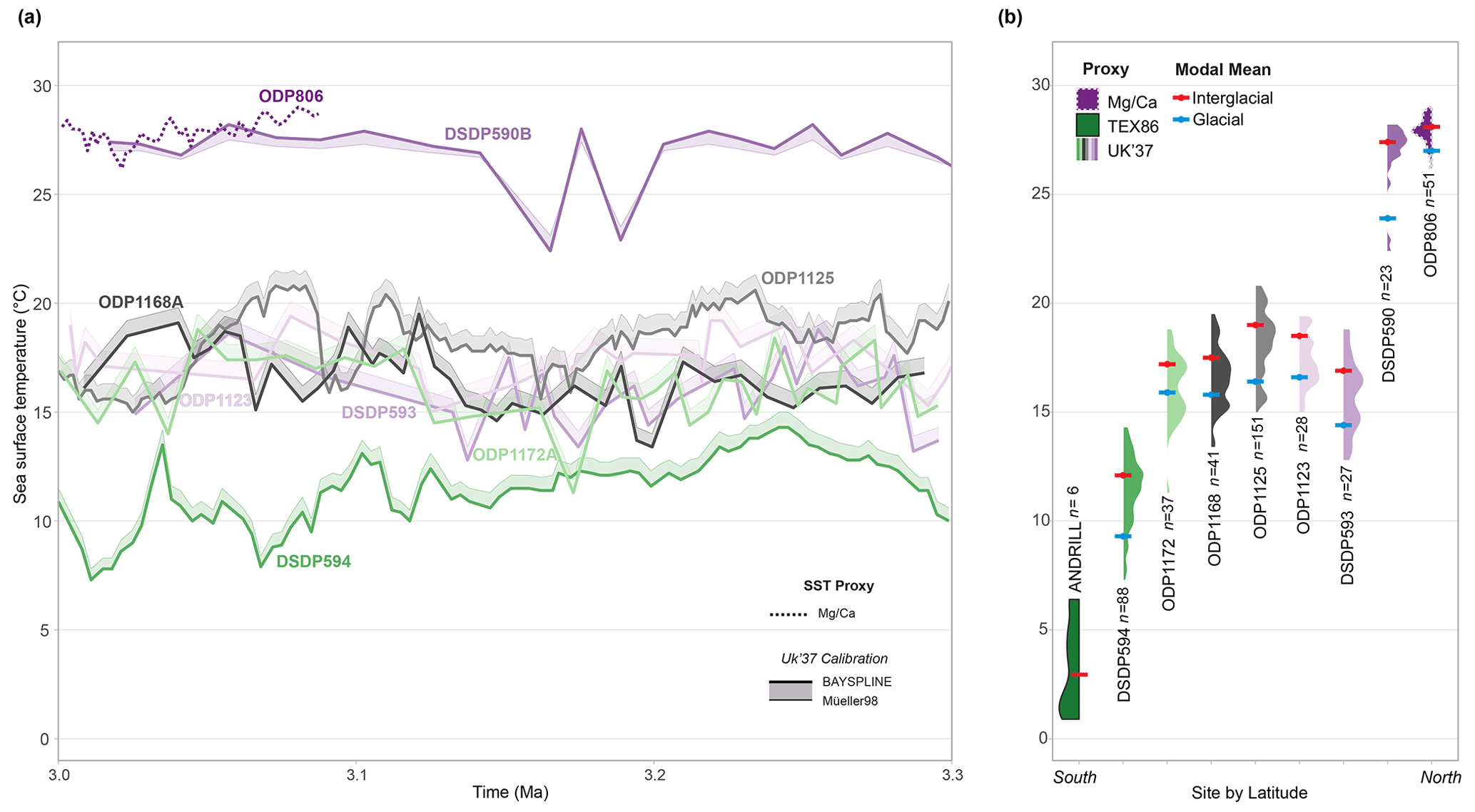
Figure 4 Time series and SST distribution for the mPWP (3.3–3.0 Ma) records. (a) U${}_{\mathrm{37}}^{\mathrm{K}{}^{\prime }}$ – SST calibrations of BAYSPLINE (solid; Tierney and Tingley, 2018), with the difference to Müller et al. (1998) shaded are plotted for all time series, with ODP 806 (Mg/Ca SST derived) and excluding ANDRILL (not plotted due to poor age control). (b) Probability distributions (“violin plots”) of the SST time series. Interglacial (red) and glacial (blue) modal means are also shown (Table 2; Fig. B1). Data for this plot are provided in Tables S1 and S2.

The temperature distributions for each site (excluding ANDRILL as interglacial values only) were assessed for bi-modal distribution to identify mean glacial and interglacial modes using the “noramlmixEM2comp” function in package mixtools (Benaglia et al., 2010). This employs an expectation–maximisation (EM) algorithm to fit an equal two-component mixture model, assuming normal distributions. This is an automated process (samples are not identified as glacial or interglacial) assuming equal two-part mixture and normal distributions of these mixtures. While the accuracy of these results is dependent on the assumptions applied here – that the glacials and interglacials present a normal distribution and have an equal bi-modal component – it is a systematic approach that applies statistical analysis to objectively identify the variance within the data and attribute it to glacial and interglacial conditions recorded in the data (Fig. B2). We acknowledge that this is an imperfect approach. However, we consider that this reduces bias introduced when visually selecting interglacial or glacial samples reliant on discrete values or temporal constraints (the latter are age model dependent). Secondly, this reduces emphasis on extreme warming during some interglacials of the mPWP and varying responses of the sites so we can be more confident that the SSTs are reflective of the broader climate conditions of the mPWP. These interglacial modes are used for plotted and tabulated comparisons to the UKESM and NZESM projections presented in the results below. Uncertainty (1σ) associated with the U${}_{\mathrm{37}}^{\mathrm{K}{}^{\prime }}$-BAYSPLINE calibration is ±1.4 ^∘C below ∼23.4^∘ and non-linear above (Tierney and Tingley, 2018). Therefore, the higher SSTs of DSDP 590 have a higher uncertainty (average of ±2.4 ^∘C; Table 2). The uncertainties for all proxy SSTs are taken as the mean of all sites (±1.5 ^∘C) for absolute SST and when referenced to pre-industrial HadISST (Table 2).

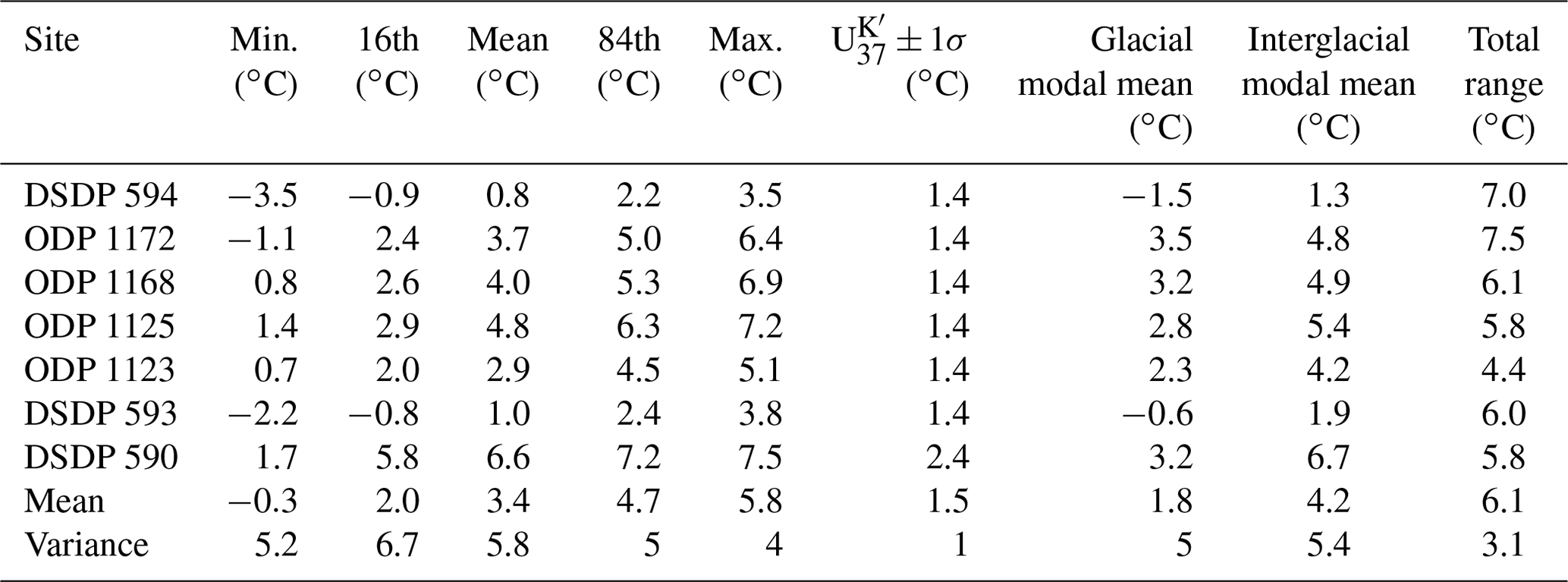
Table 2 Statistical distribution of mPWP SST anomalies relative to HadISST (1870–1879 CE) using U${}_{\mathrm{37}}^{\mathrm{K}{}^{\prime }}$ BAYSPLINE-derived SSTs. Reported minimums, 16th percentile, mean (50th percentile), 84th percentile and maximum SST anomalies are shown with U${}_{\mathrm{37}}^{\mathrm{K}{}^{\prime }}$ BAYSPLINE-reported 1σ uncertainty. Glacial and interglacial modal means are calculated as described in methods, and the total range is calculated as the difference between maximum and minimum temperature.

3 Results

3.1 Mid-Pliocene warm period sea-surface temperature signature

With respect to pre-industrial temperatures (HadISST), mean site SST anomalies for the mid-latitudes (45 to 30^∘ S) range from 0.8 to 6.6 ^∘C with a likely (16th–84th percentile) range of 2–4.7 ^∘C (3.4 ^∘C average for all sites). Minimum SST anomalies for the sites range from −3.5 to 1.7 ^∘C (−0.3 ^∘C average for all sites) and maximum SST anomalies range from 3.5 to 7.5 ^∘C (5.8 ^∘C average of all sites; Table 2). Interglacial modal mean anomalies, used in this study as moderate warm conditions, range between 1.3 and 5.4 ^∘C (average 4.2 ^∘C), warmer than HadISST for the south-west Pacific mid-latitude sites.

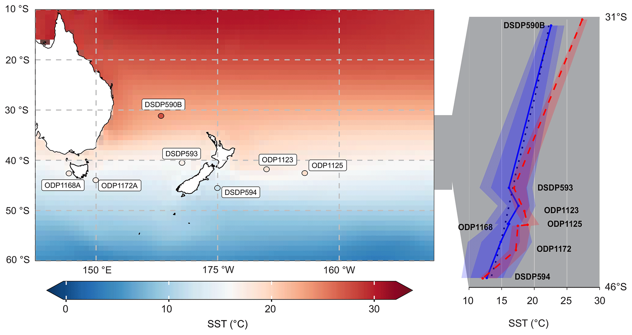
Figure 5 Absolute SST for ensemble mean core PlioMIP experiments with mPWP site mean interglacial SST plotted using the same temperature scale. SSTs between 31 and 46^∘ S are shown in the right panel for PlioMIP latitudinal mean (blue dotted), PlioMIP site specific (blue solid) with transparent blue shading for minima–maxima and heavier blue shading for ±1 SD (standard deviation) of the PlioMIP ensemble and mPWP site specific (red dashed) with mean–maxima shaded in red.

The sites presented in this study are sampled over glacial–interglacial cycles for which the total glacial–interglacial amplitude of SSTs range from ∼4.4 to ∼7.5 ^∘C (Fig. 4; Table 2; excluding ANDRILL and ODP 806). Interglacial and glacial modal means determined by the bimodal statistical analysis (Sect. 2.3) are generally comparable to the 16th and 84th percentile (within ∼1 ^∘C), highlighting that these modes are reflective of the likely range rather than accounting for extreme values representing the tails of the p distribution used to estimate the total glacial–interglacial amplitude range, which has a mean of 6.1 ^∘C (Table 2). The difference between glacial and interglacial modal means is approximately half that of the total glacial–interglacial amplitude (∼3 ^∘C; Table 2). The meridional gradients for mean glacials or interglacials do not differ significantly but do show a flattened gradient for interglacial modal means between site DSDP 590 and ODP 806 (30–0^∘ S; Fig. 4b) due to the low SST distribution of site ODP 806.

The sites warm (∼0–20 ^∘C) from the pole to site ODP 1125 (north Chatham Rise), before a reduction in SSTs are seen at sites ODP 1123 (offshore Chatham Rise) and DSDP 593 (eastern Tasman Sea), then returning to high temperatures of > 25 ^∘C at sites north of 32^∘ S (DSDP 590 and ODP 806), which show comparable peak temperatures (Fig. 4). While latitude is generally correlated with SST, surface water mass and regional currents alter this relationship. Site DSDP 594 south of the Subtropical Front in surface Subantarctic Water is noticeably colder than sites situated either within (ODP 1172) or just north of (ODP 1168, ODP 1125 and ODP 1123) the Subtropical Front. However, current proximity to the Subtropical Front does not appear to be a main driver either.

DSDP 593 and DSDP 594 (north and south of the Subtropical Front) show the least warming above pre-industrial conditions, but interglacial modal means still warm 1–2 ^∘C. Sites that show significant interglacial modal mean warming above the global mPWP average are offshore Tasmania (ODP 1168 and ODP 1172) and site ODP 1125 (northern Chatham Rise), which all display warming between 4.8 and 5.4 ^∘C; DSDP 590 (north Tasman Sea) presents extreme warming of 6.7 ^∘C (Table 2).

3.2 Global climate models

3.2.1 PlioMIP

Standardised boundary conditions used by all 16 models participating in PlioMIP, termed the PlioCore experiment (Haywood et al., 2016, 2020), are based on the latest PRISM4 climate reconstruction for MIS KM5c (Dowsett et al., 2016). Data presented here are the multi-model mean of PlioCore (Haywood et al., 2020) with site-specific SSTs extracted and referenced to the HadISST pre-industrial reanalysis (NCAR, 2022) for comparison to the mPWP proxy SSTs (Table 3; Fig. 5). Due to the poor spatial distribution of this study (although considerably higher than previous studies in the region), we are unable to sum the temperature distribution over latitudinal ranges of 30^∘ for comparison to meridional gradients reported elsewhere (e.g. Haywood et al., 2020; McClymont et al., 2020). However, we provide a comparison of mPWP site data to PlioMIP latitudinal averages (1^∘ resolution) between longitudes 140^∘ E and 160^∘ W, alongside site-specific SST from the PlioMIP experiment (Haywood et al., 2020).

Table 3 Summary site mean SST (^∘C) for HadISST (1870–1879 CE), PlioMIP (multi-model mean) and interglacial modal mean mPWP U${}_{\mathrm{37}}^{\mathrm{K}{}^{\prime }}$ BAYSPLINE-derived SST (this study), as well as SST anomaly (relative to HadISST) for PlioMIP and mPWP.

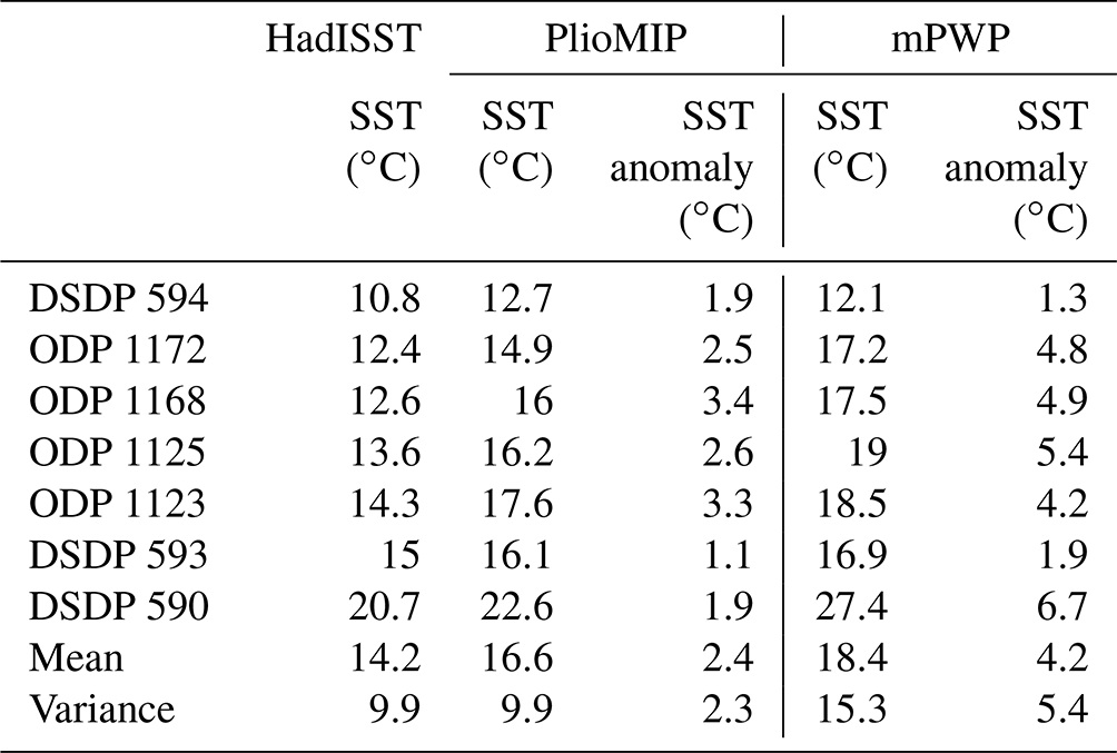
Specific site warming for PlioMIP does not vary significantly from the meridional gradient except for ODP 1123 (Fig. 5b). Sites ODP 1123, DSDP 593 and DSDP 594 all present SST anomalies within 1 ^∘C for PlioMIP and mPWP (Table 3). However, on average for the sites, the PlioMIP SST anomaly is 2.4 ^∘C, while that of mPWP is 4.2 ^∘C (Table 3).

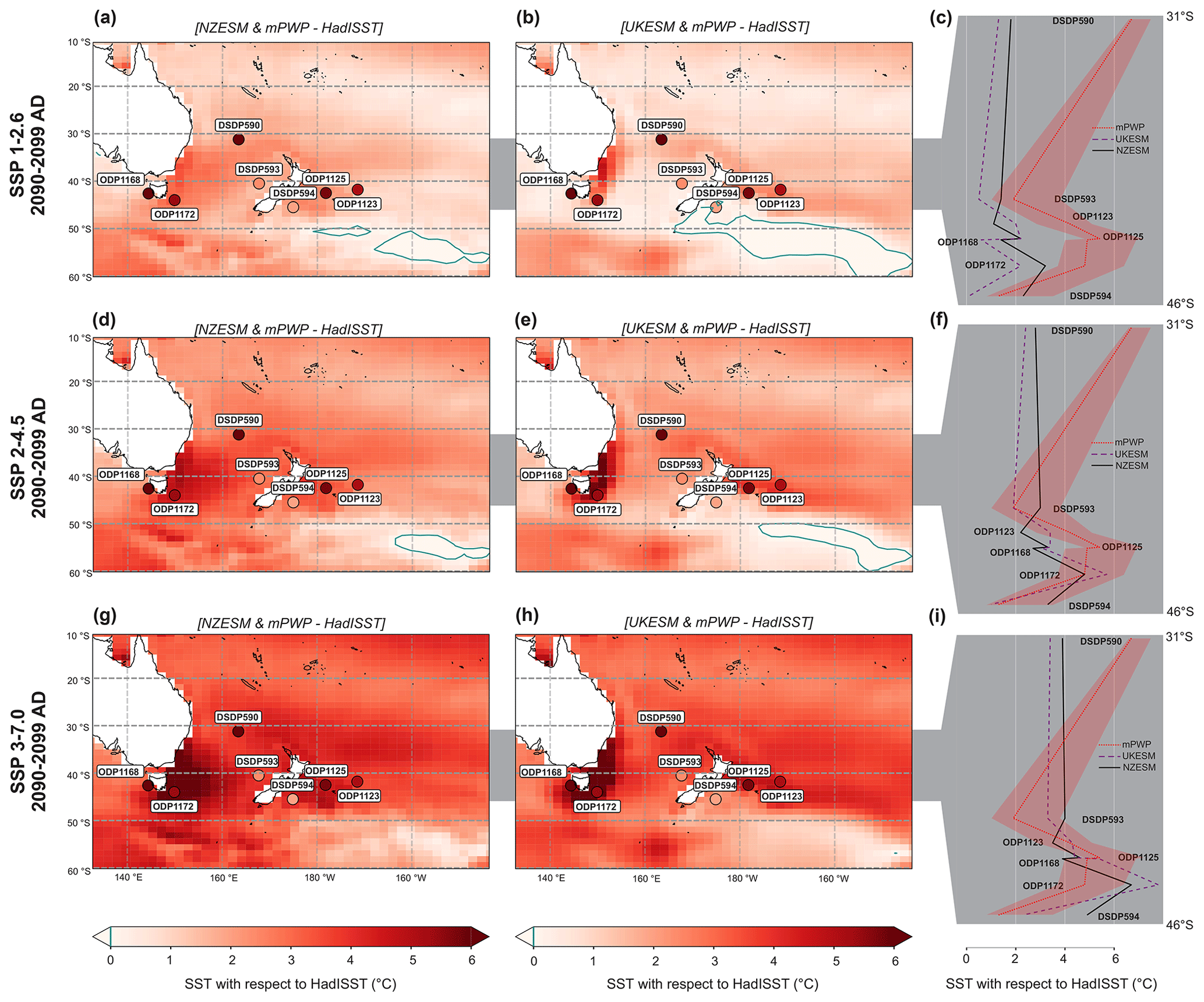
Figure 6 Regional SST anomalies to HadISST (1870–1879 CE) for SSP1–2.6 (a–c), SSP2–4.5 (d–f) and SSP3–7.0 (g–i) in 2090–2099 CE compared to mPWP site mean interglacial SST anomalies (filled circles using same colour scale as map). (a, d, g) are NZESM, (b, e, h) are UKESM and (c, f, i) are site SST anomalies between 31 and 46^∘ S for mPWP (red dotted), UKESM (purple dashed) and NZESM (black solid).

3.2.2 Future Earth system model simulations

On average, NZESM simulations show higher warming than the coarser-resolution UKESM in all scenarios presented here (Table 4; Fig. 6). However, for the sites investigated, UKESM simulations show more variability between sites due to minimal warming at ODP 594 and extreme warming at site ODP 1172 (Table 4; Fig. 6). As for proxy data in the previous section, statistical summaries refer to the mid-latitude sites (excluding ANDRILL and ODP 806).

Table 4 Site annual mean SST anomalies (^∘C) for UKESM and NZESM with respect to HadISST (1870–1879 CE) for SSP1–2.6, SSP2–4.5 and SSP3–7.0 at 2095 CE (2090–2099 CE). Global SST for the mPWP refers to the compilation by McClymont et al. (2020).

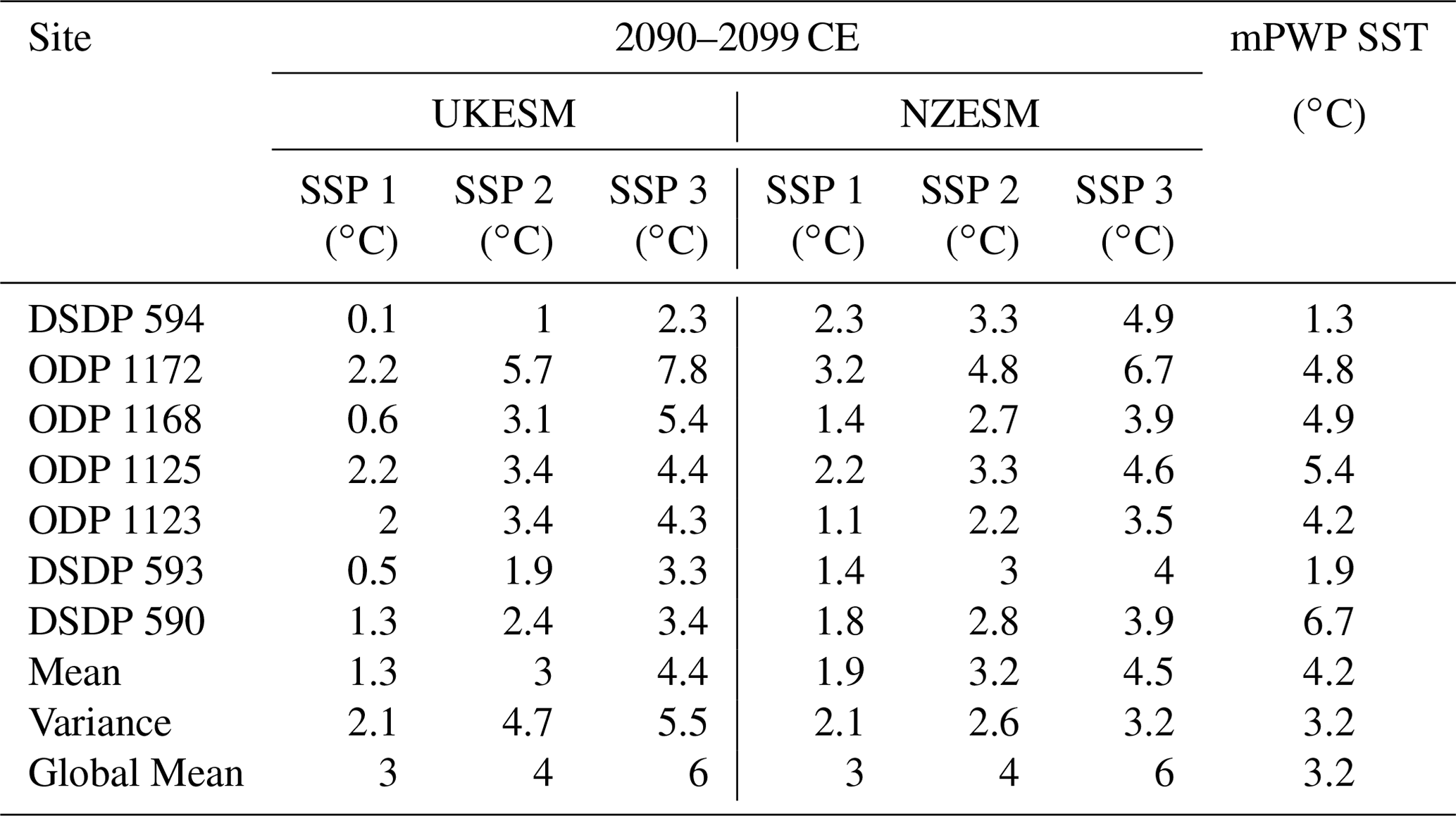
Projections for 2090–2099 CE for SSP1–2.6, SSP2–4.5 and SSP3–7.0 show a stable pattern of warming for both models (Table 4; Fig. 6). However, warming at sites ODP 1172, ODP 1168, ODP 1123 and ODP 1125 in UKESM simulations increases above NZESM with higher emission scenarios, while DSDP 594 and 593 remain significantly higher in NZESM simulations over UKESM (Table 4). NZESM and UKESM simulations for SSP3–7.0 have similar mean warming (+4.5 and +4.4 ^∘C respectively) to the mPWP (+4.2 ^∘C), with the means strongly biased by differences in DSDP 594, 593 and 590 (Table 4). The intense warming recorded at site DSDP 590 during the mPWP is particularly visible in latitudinal gradient comparisons (Fig. 6c, f and i) and highlights the importance of comparing site-specific data.

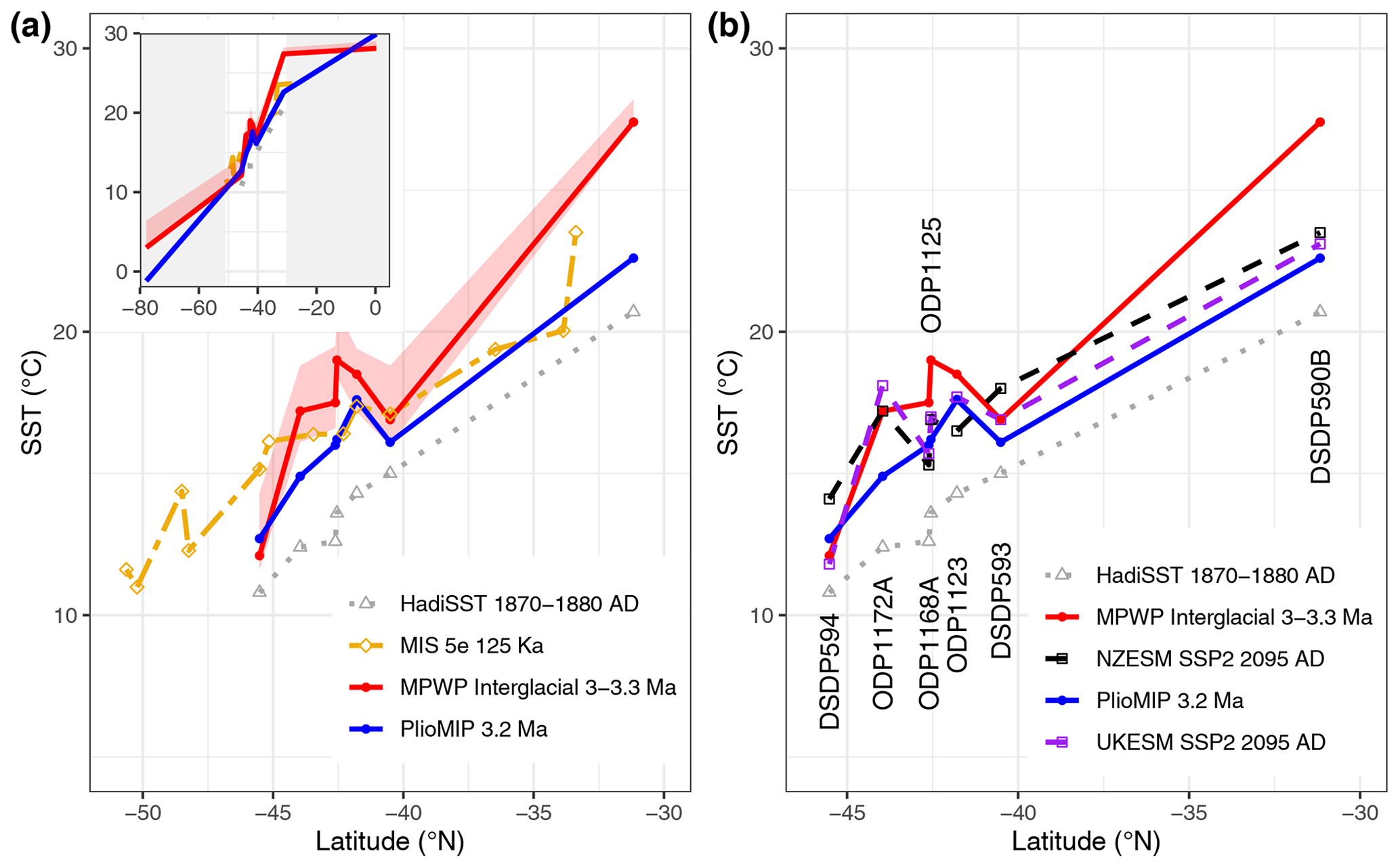
Figure 7 Absolute SSTs as a latitudinal transect of the south-west Pacific with (a) HadISST (NCAR, 2022), mPWP interglacial (solid red with the red ribbon showing mean to maximum SSTs), PlioMIP multi-model mean (solid blue) and MIS 5e (∼125 ka; dashed yellow; Cortese et al., 2013) and (b) HadISST (dotted grey; NCAR, 2022), mPWP interglacial modal mean (solid red), NZESM (dashed black) and UKESM (dashed purple) for SSP2–4.5 2090–2099 CE (Williams et al., 2016; Sellar et al., 2019).

4 Discussion

4.1 Pliocene analogue

The mPWP encompasses several glacial cycles throughout the 300 kyr, with variable climate conditions (insolation, CO₂ and tropical SST; Fig. 2). Many studies have therefore focussed on a single interglacial (MIS KM5c) as insolation values are near identical to today (Laskar et al., 2004; Haywood et al., 2020; McClymont et al., 2020). However, this requires confidence in age models and ultimately tuning of records. The approach taken here, of assessing glacial and interglacial characteristics spanning the whole mPWP interval, aims to smooth glacial and interglacial extremes and represent the more “likely” climate conditions for equilibrium glacial and interglacial states across the region. Interglacial SST site modal means (this study) between 30 and 45^∘ S average at +4.2 ^∘C (Table 2) for global SST estimates of 3.2–3.4 ^∘C (McClymont et al., 2020). In comparison, for the same sites, PlioMIP SSTs average 2.4±2.1 ^∘C (MIS KM5c; Haywood et al., 2020; Table 3), with a global multi-mode median of 3.0 ^∘C (10th–90th percentiles: 2.1–4.8 ^∘C; Haywood et al., 2020). Thus, this study demonstrates an amplified warming signal in the south-west Pacific relative to the global mean temperature that is not displayed in the PlioMIP simulations. Likewise, the mean of glacial modes is +2 ^∘C with reference to HadISST (Table 2), where glacial conditions of the mPWP are often considered comparable to pre-industrial (Lisiecki and Raymo, 2005), which is however, poorly studied. The comparable SSTs for sites with previously published values for MIS KM5c provide confidence in the approach of representing interglacial modal means used in this study and highlights the importance of regional variability in site selection to determine regional response (Fig. 7a). While we acknowledge the sites provided in this study are still spatially limited, they provide a significant increase to the resolution of sampling in this area for the mPWP.

Site DSDP 590 (northern Tasman Sea), which is currently north of the Tasman Front outlet of the EAC, presents the highest SSTs. The location of the Tasman Front is controlled by the northern tip of New Zealand's North Island, which was at a slightly lower latitude in the Pliocene (Strogen et al., 2022), which may have allowed for a more northern Tasman Front, directing warmer waters across site DSDP 590. Alternatively, the warming at DSDP 590 may be explained by a broadening and invigoration of the Tasman Front, which may be at the expense of flow to the EAC extension (Hill et al., 2011). While a strengthening of the EAC is expected, the magnitude and distribution of this strengthening is argued (Hill et al., 2011). This circulation shift could also account for a lower degree of warming observed in the mPWP at site ODP 1172, situated in the southern extent of the EAC. Furthermore, redirected flow through the Tasman Front, which ultimately bathes the Chatham Rise, may account for the high degree of warming displayed by sites ODP 1123 and ODP 1125 (Table 2).

Furthermore, previous studies of the Last Interglacial (MIS 5e; 125 ka) suggest that the warming of southern and eastern New Zealand (specifically based on data from site ODP 1123) may be a result of an increased and extended flow of the EAC becoming entrained in the Subtropical Front that would bathe the Chatham Rise sites (Fig. 7a; Cortese et al., 2013). The results presented here support a strengthening of the EAC and outlets relative to pre-industrial and modern conditions, which are consistent with palaeo studies of Late Pleistocene interglacials (Bostock et al., 2015; Cortese et al., 2013) and suggest these currents may have multiple ways of operating under warmer climates. Indeed, modern EAC transport and outlets are underestimated by most models (Chiswell et al., 2015; Sen Gupta et al., 2016, 2021).

Palaeo–model comparison

Warming during the interglacial modal means of the mPWP can be simplified as >4 ^∘C above pre-industrial temperatures in five of the seven mid-latitude sites across the region, with two sites (DSDP 593 and DSDP 594) showing moderate warming (<2 ^∘C; Table 2). This pattern is broadly reflected in both UKESM and NZESM projected scenarios explored here, with closer fit under the middle-of-the-road emission scenario (Figs. 6 and 7b; Table 4). NZESM and UKESM show a general trend (for the seven mid-latitude sites) of closer correlation to mPWP at lower temperature sites with increasing underestimation at sites with higher SSTs for all scenarios except for SSP3–7.0 (Fig. 6). These low-temperature sites (DSDP 593 and DSDP 594) are also the two sites where UKESM provides systematically warmer values than NZESM (Fig. 6; Table 4).

The key differences between the UKESM and NZESM can be summarised by more-distributed, region-wide warming in the NZESM, with reduced warming along the EAC and offshore eastern New Zealand (Fig. 6). The pattern of the NZESM SST field reflects local oceanographic grid refinement, which improves the fidelity of complex regional current transport and the representation of ocean fronts (Behrens et al., 2020). The concentrated regionally limited warming of the UKESM is less consistent with the mPWP signature of warming across the region (Fig. 6). Specifically, NZESM presents lower SSTs for the EAC relative to the UKESM, which is more consistent with SSTs at site ODP 1172 during the mPWP (Fig. 6). This also corroborates the apparent intense warming observed at site DSDP 590 in the northern Tasman Sea during the mPWP because of increased flow eastward to the Tasman Front at the expense of an invigorated EAC; however, this may also reflect the palaeogeographic positioning of site DSDP 590 and the Tasman Front (Strogen et al., 2022). Significantly, while the NZESM produces a Subtropical Front further south than the UKESM, bathing DSDP 594 in warmer waters, this does not extend to the eastern Chatham Rise sites, which is not consistent with mPWP observations (Fig. 6g–i). Lastly, we note that warming at site ODP 1168 (south-west Tasmania) is comparable to site ODP 1172 (south-east Tasmania; EAC) during the mPWP, which is inconsistent with both NZESM and UKESM (Fig. 6).

Modelled SSTs at the sites show increased variability under higher-emission scenarios (Fig. 6), more comparable to the range and magnitude of mPWP observations; however, this is driven by closer values at DSDP 590 and it tends to overestimate SSTs at the other sites (Fig. 6; Tables 4 and S5). Rather, for both UKESM and NZESM, SSP2–4.5 for 2090–2099 CE shows the least deviation to all sites reconstructed for the mPWP (Figs. 6d–f and 7b). While the magnitude of warming changes significantly with SSP projections, we consider both UKESM and NZESM to produce a pattern of warming consistent with site observations of the mPWP.

Considering regional SSTs in the meridional context, we have compared HadISST, mPWP and PlioMIP with Last Interglacial MIS 5e (Fig. 7a) and ESM scenarios for SSP2–4.5 by 2090–2099 CE (Fig. 7b). The glacial and interglacial gradients of the mPWP are relatively consistent and show a much steeper gradient in comparison to the interglacial MIS 5e (+1–2 ^∘C) and pre-industrial HadISST (Fig. 7a), while future ESM projections for SSP2–4.5 2090–2099 CE (as the closest scenario to mPWP) show a much more comparable distribution with the mPWP (Fig. 7b).

4.2 Global and regional warming

In comparing our interglacial modal mean mPWP SSTs, reconstructed using organic biomarker proxies, in conjunction with data sampled for the same sites from transient ESM simulations to run to 2100 CE, we acknowledge that the ESM values do not reflect the future equilibrium temperature responses for these south-west Pacific sites. However, in most cases, average regional temperatures at the sites studied are expected to increase beyond 2100 CE as longer duration feedback in the Earth climate system plays out. To consider the difference between equilibrium and transient climates, we discuss the variance of global and regional SSTs between palaeo and future scenarios.

Global SSTs during mPWP interglacials are ∼3 ^∘C above pre-industrial temperatures (Masson-Delmotte et al., 2013; Dowsett et al., 2016; McClymont et al., 2020; Haywood et al., 2020), comparable to expected warming (2.1–3.5 ^∘C) for SSP2–4.5 by 2100 CE (IPCC, 2022). The pattern and magnitude of regional warming is similar between the mPWP and ESM simulations under SSP2–4.5 (Table 4; Figs. 6 and 7b); however, the global warming generated by the ESMs under SSP2–4.5 is 4 ^∘C. Thus, while these mPWP proxy SSTs present a higher degree of warming than the global, the same degree of warming from UKESM and NZESM requires a 1 ^∘C higher global temperature increase.

The ECS of the UKESM (and NZESM) is 5.4 ^∘C (Sellar et al., 2019; Senior et al., 2020), which exceeds that of estimates for the mPWP of 2.6–4.8 ^∘C (MIS KM5c; Haywood et al., 2020) and far exceeds that of the likely range (2.5–4 ^∘C) for the CMIP6 ensemble (Forster et al., 2021). This is of importance because the Southern Ocean has long been identified as having significant deviation from models to observations and it is uncertain whether high ECS models (linked to shortwave cloud feedback; Zelinka et al., 2020) act to better estimate observations (Schuddenboom and McDonald, 2021). Here, we show that the high ECS simulations of NZESM and UKESM present a comparable warming signature seen during the mPWP in the south-west Pacific, as opposed to the lower ECS PlioMIP simulations (Fig. 7b). These results demonstrate that while higher ECS models do produce a more-extreme regional temperature response under transient climates and ∼100-year timescales, they require a higher degree of global warming, suggesting that longer-term feedback including ice dynamics may play a significant role in accurately determining committed warming, particularly for this region in proximity to Antarctica and the Southern Ocean. Furthermore, the use of lower ECS models (e.g. the majority of the CMIP6 ensemble) for regional downscaling in the south-west Pacific may be underestimating the amplified warming signal we see in the mPWP and ESM SSP2–4.5 scenarios (Appendix C).

5 Conclusions

The regional expression of warming differs from the global average on a variety of timescales and has significant implications for the frequency and extent of climate-induced hazards related to weather, sea-level rise and socio-economic factors. Our mPWP proxy SST reconstructions for interglacial modal means show warming at sites across the south-west Pacific averaged at 4.2 ^∘C, that is 1–2 ^∘C above global warming (Masson-Delmotte et al., 2013). This mPWP SST signature contains significant regional variability that is not seen in the PlioMIP multi-model mean and exceeds the south-west Pacific PlioMIP average of 2.4 ^∘C (Haywood et al., 2020); however, it does replicate warming at the three sites used in the PRISM climate reconstruction (Dowsett et al., 2016; McClymont et al., 2020).

NZESM and UKESM show relatively consistent warming under low- and high-emission pathway simulations, but the NZESM presents slightly warmer site averages in all scenarios. The most comparable warming to mPWP by the ESMs is for 2090–2099 CE under the SSP2–4.5 scenario that is expected to reach 2.1–3.5 ^∘C globally by 2100 CE (IPCC, 2022). However, the global warming for these ESMs under this pathway is ∼4 ^∘C, which relates to the high ECS of the models. This suggests that high ECS models better replicate the regional warming signature in the south-west Pacific and that low ECS models in the CMIP6 ensemble may underestimate warming in the south-west Pacific. Ultimately, testing of longer-term scenarios using NZESM to accommodate for long feedback, for instance, potentially including a quantitative ice-sheet model (Smith et al., 2021), would provide insight into the impacts of warming on ocean currents in the south-west Pacific and determine the effect of transient and equilibrium climate responses.

Palaeoclimate reconstructions, such as those presented in this study, act as the only available evidence of equilibrium climate responses to conditions predicted for the near-future. While equilibrium climate states are not directly comparable to the transient future projections, expected sustained warming may result in comparable conditions.

Appendix A

Lipid biomarkers were analysed in the Organic Geochemistry Laboratory at GNS Science as reported in Naeher et al. (2012, 2014) and Ohkouchi et al. (2005) with modifications. In brief, freeze-dried and homogenised sediment samples (10–17 g) were extracted four times with dichloromethane / methanol (DCM / MeOH; 3:1, v:v) by ultrasonication for 20 min each time. Elemental sulfur was removed by activated copper. The total lipid extracts (TLEs) were divided into three fractions via liquid chromatography over silica columns using n-hexane (F1), n-hexane / DCM (1:2, v:v; F2) and DCM / MeOH (1:1, v:v; F3) respectively.

The F2 fractions containing alkenones were analysed using gas chromatography mass spectrometry (GC-MS) on an Agilent 7890A GC System, equipped with an Agilent J & W HP-1ms capillary column (60 m × 0.32 mm inner diameter, i.d. × 0.25 µm film thickness, f.t.) and connected through a splitter to an Agilent 5975C inert mass selective detector mass spectrometer and flame ionisation detector (FID). The oven was heated from 70 to 280 ^∘C at 20 ^∘C min⁻¹, then at 4 ^∘C min⁻¹ to 320 ^∘C and held isothermal for 20 min with a total run time of 40.5 min. Helium was used as carrier gas with a constant flow of 1.0 mL min⁻¹. Samples (1 µL) were injected splitless at an inlet temperature of 320 ^∘C. The MS was operated in electron impact ionisation mode at 70 eV using a source temperature of 230 ^∘C. For alkenone identification, the MS was operated in simultaneous full scan and single ion monitoring (SIM) mode at $m/z$ 55, 58, 97, 109.1, 526.5, 528.5 and 530.5. Alkenones were quantified using the FID.

Glycerol dialkyl glycerol tetraethers (GDGTs), present in the F3 fractions, were dissolved in n-hexane/isopropanol (99:1, v:v) and filtered with 0.45 µm PTFE filters prior to liquid chromatography mass spectrometry (LC-MS) analysis at the University of Hokkaido, Japan. GDGTs were analysed on an Agilent 1260 high-performance LC system coupled to an Agilent 6130 Series quadrupole MS. Separation was achieved using a Prevail Cyano column (2.1×150 mm, 3 µm; Grace Discovery Science, USA) maintained at 30 ^∘C following the method of Hopmans et al. (2004) and Schouten et al. (2007). Conditions were as follows: flow rate 0.2 mL min⁻¹, isocratic with 99 % n-hexane and 1 % isopropanol for the first 5 min followed by a linear gradient to 1.8 % isopropanol over 45 min. Ionisation was achieved using atmospheric pressure positive ion chemical ionisation. The spectrometer was run in selected ion monitoring mode ($m/z$ 743.8, 1018, 1020, 1022, 1032, 1034, 1036, 1046, 1048, 1050, 1292.3, 1296.3, 1298.3, 1300.3 and 1302.3). Compounds were identified by comparing mass spectra and retention times with those in the literature (Hopmans et al., 2004).

The U${}_{\mathrm{37}}^{\mathrm{K}{}^{\prime }}$ index is defined based on the relative abundance of the C_37:2 and C_37:3 alkenones according to Prahl and Wakeham (1987) as follows:

$$\begin{array}{}\text{(A1)}& {\mathrm{U}}_{\mathrm{37}}^{\mathrm{K}{}^{\prime }}=\left[{\mathrm{C}}_{\mathrm{37}:\mathrm{2}}\right]/\left(\left[{\mathrm{C}}_{\mathrm{37}:\mathrm{2}}\right]+\left[{\mathrm{C}}_{\mathrm{37}:\mathrm{3}}\right]\right).\end{array}$$

We used the calibration of Müller et al. (1998) and BAYSPLINE (Tierney and Tingley, 2018) to reconstruct SSTs from the U${}_{\mathrm{37}}^{\mathrm{K}{}^{\prime }}$ index.

The TEX₈₆ index is based on the relative distribution of isoprenoidal glycerol dialkyl glycerol tetraethers (isoGDGTs) in marine sediments, originally defined by Schouten et al. (2002):

$$\begin{array}{}\text{(A2)}& \begin{array}{rl}& {\mathrm{TEX}}_{\mathrm{86}}=\\ & {\displaystyle \frac{\left[\mathrm{GDGT}\text{-}\mathrm{2}\right]+\left[\mathrm{GDGT}\text{-}\mathrm{3}\right]+\left[\mathrm{GDGT}\text{-}{\mathrm{4}}^{\prime }\right]}{\left[\mathrm{GDGT}\text{-}\mathrm{1}\right]+\mathit{\left\{}\mathrm{GDGT}\text{-}\mathrm{2}\right]+\mathit{\left\{}\mathrm{GDGT}\text{-}\mathrm{3}\mathit{\right\}}+\mathit{\left\{}\mathrm{GDGT}\text{-}{\mathrm{4}}^{\prime }\mathit{\right\}}}}\end{array},\end{array}$$

where GDGT-1, GDGT-2 and GDGT-3 are characterised by one, two and three cyclopentane moieties and cren^′ is the regioisomer of crenarchaeol. This index derived from core-top samples was calibrated to SSTs using linear regressions as proposed by Schouten et al. (2002) and Kim et al. (2010).

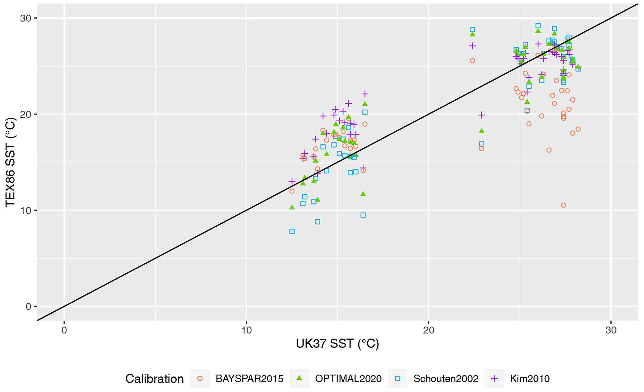
Figure A1 Comparison between U${}_{\mathrm{37}}^{\mathrm{K}{}^{\prime }}$-derived SST using BAYSPLINE with TEX₈₆ index SST calibrations of Schouten et al. (2002), Kim et al. (2010), Dunkley Jones et al. (2020) and Tierney and Tingley (2015).

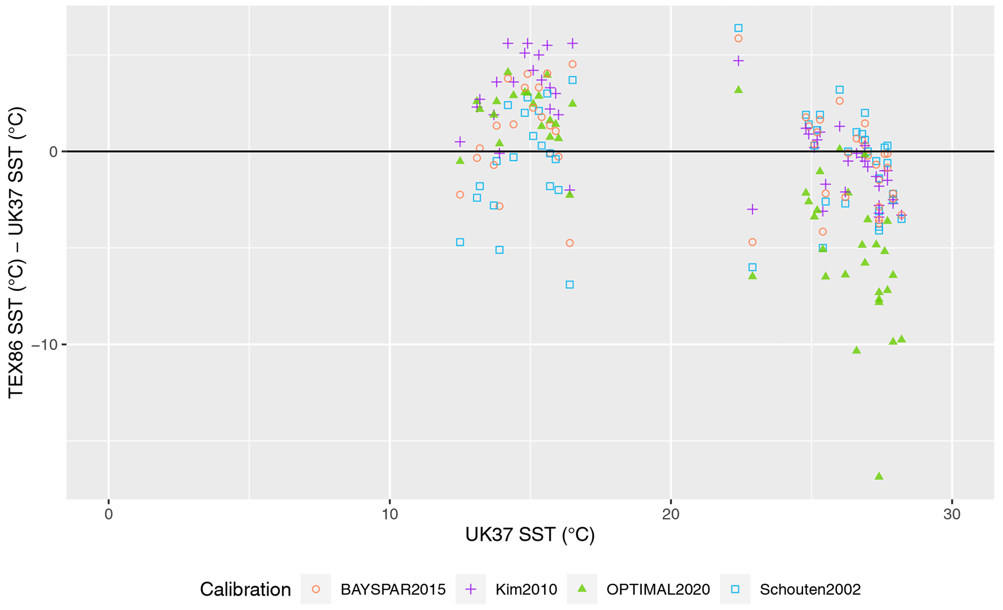
Figure A2 Comparison between U${}_{\mathrm{37}}^{\mathrm{K}{}^{\prime }}$-derived SST using BAYSPLINE with TEX₈₆ index SST calibrations of Schouten et al. (2002), Kim et al. (2010), OPTIMAL (Dunkley Jones et al., 2020) and BAYSPAR (Tierney and Tingley, 2015).

To test the reliability of reconstructed SSTs and to increase confidence in the choice of the applied calibrations, we have compared U${}_{\mathrm{37}}^{\mathrm{K}{}^{\prime }}$ and TEX₈₆ SST at two sites. While U${}_{\mathrm{37}}^{\mathrm{K}{}^{\prime }}$ SSTs using the BAYSPLINE (Tierney and Tingley, 2018) do yield slightly cooler temperatures (up to 0.7 ^∘C) at higher-latitude sites than the calibration of Müller et al. (1998), the TEX₈₆ SSTs differ by +6.4 to −16.9 ^∘C depending on the calibration used (Figs. A1 and A2). This proxy may be compromised at sites with high soil organic matter inputs (Hopmans et al., 2004) and high contributions of sedimentary GDGTs (Pancost et al., 2001; Zhang et al., 2011) which is considered negligible in open-marine environments. Other non-temperature controls such as oxygen concentrations, growth phases and nutrient cycling may be introduced in upwelling zones but are not able to be addressed here due to limited understanding of these effects (Elling et al., 2014; Qin et al., 2015; Hollis et al., 2019). Non-linear calibrations such as the TEX${}_{\mathrm{86}}^H$ index (Kim et al., 2010) were developed to extend the calibrated SST range of the previous calibrations; however, this may underestimate SSTs in ancient greenhouse climates (Tierney and Tingley, 2015; O'Brien et al., 2017; Hollis et al., 2019) and a non-linear relationship contradicts available experimental evidence suggesting a linear relationship with SST (Pitcher et al., 2010; Schouten et al., 2013; Elling et al., 2014). Therefore, a Bayesian approach (BAYSPAR; Tierney and Tingley, 2015) was developed to consider spatially varying uncertainty derived from a widely used modern SST distribution. Additionally, a new machine-learning approach (OPTiMAL: Optimised Palaeothermometry from Tetraethers via MAchine Learning) aims to address uncertainty in the method application to palaeo SST and determine SST beyond the modern range (>30 ^∘C; Dunkley Jones et al., 2020). In comparing the two independent biomarker proxies of derived SST using U${}_{\mathrm{37}}^{\mathrm{K}{}^{\prime }}$ – BAYSPLINE with TEX₈₆ calibrations of Schouten et al. (2002), Kim et al. (2010), Tierney and Tingley (2015) and Dunkley Jones et al. (2020), we find that all calibrations are comparable ($\sim \pm \mathrm{5}$ ^∘C) but the BAYSPAR approach of Tierney and Tingley (2015) displays the closest values to U${}_{\mathrm{37}}^{\mathrm{K}{}^{\prime }}$-BAYSPLINE (Fig. A1 and A2; Table A1). Notably, the calibrations of Schouten et al. (2002), Kim et al. (2010) and BAYSPAR (Tierney and Tingley, 2015) show less scatter at higher temperatures (>25 ^∘C; Fig. A1), while the OPTIMAL calibration (Dunkley Jones et al., 2020) presents offsets of up to −15 ^∘C (Fig. A2) in comparison to U${}_{\mathrm{37}}^{\mathrm{K}{}^{\prime }}$-BAYSPLINE.

The TEX₈₆ calibration of Tierney and Tingley (2015; BAYSPAR) shows the closest values to the U${}_{\mathrm{37}}^{\mathrm{K}{}^{\prime }}$ – SST BAYSPLINE and lowest scatter (Figs. A1 and A2; Table A1); these are therefore selected for display in Fig. 4. In contrast, the calibration of Schouten et al. (2002) shows larger scatter in reconstructed SSTs than BAYSPAR (Figs. A1 and A2). The calibration of Kim et al. (2010) yields similar SST estimates as Schouten et al. (2002) and BAYSPAR, but seems to overestimate SSTs at lower temperatures. In contrast, OPTIMAL (Dunkley-Jones et al., 2020) appears to underestimate SSTs at higher temperatures. Importantly, the general agreement in SST reconstruction from two independent biomarker provides higher confidence in the results.

Table A1 Comparison between U${}_{\mathrm{37}}^{\mathrm{K}{}^{\prime }}$-derived SST using BAYSPLINE with TEX₈₆ index SST calibrations of Schouten et al. (2002), Kim et al. (2010), OPTIMAL (Dunkley Jones et al., 2020) and BAYSPAR (Tierney and Tingley, 2015).

Appendix B

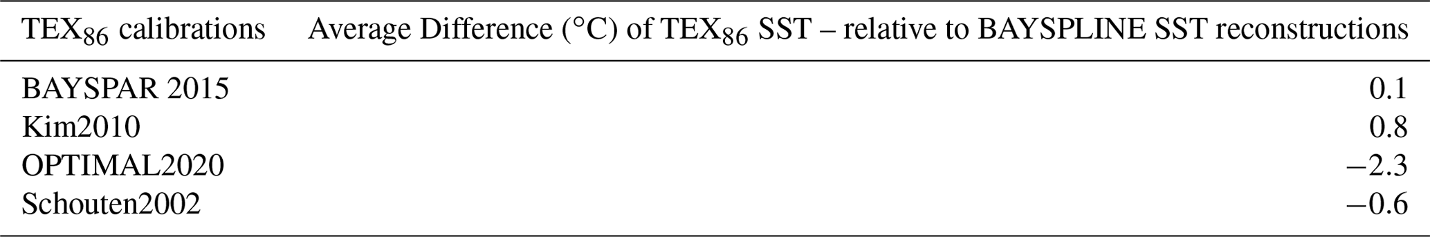
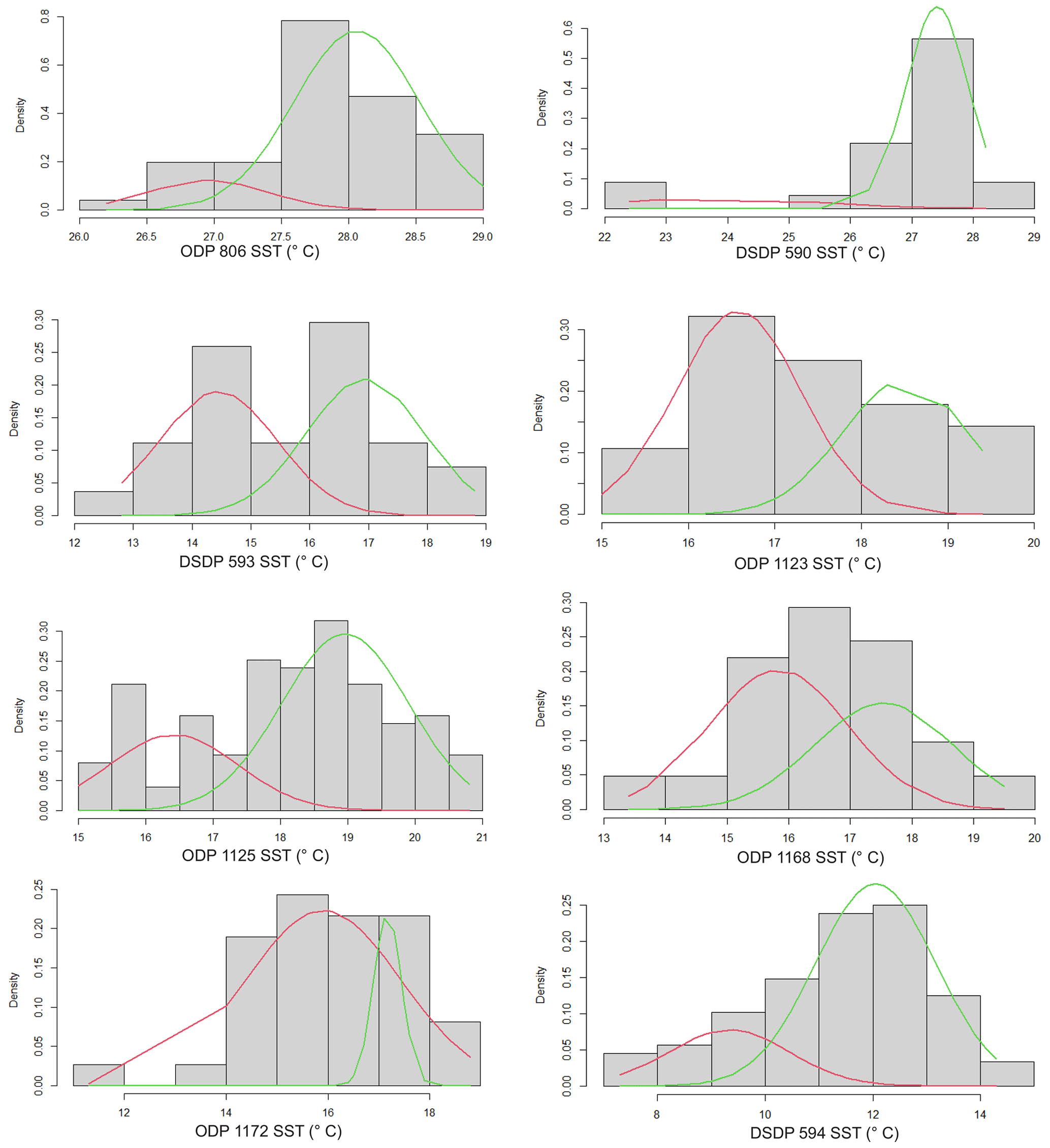
Figure B1 Bimodal analysis for each site after Benaglia et al. (2010), excluding ANDRILL as it only represents interglacial conditions, displaying density curves with calculated bimodal distributions interpreted as glacial distributions (red) and interglacial (green). Code is available.

Appendix C

Figure C1 Extended version of Fig. 6 to include a second high ECS model (CESM2: ECS 5.2–5.6 ^∘C; Danabasoglu et al., 2020) and the lowest ECS model in CMIP6 (INM: ECS 1.8 ^∘C; Volodin et al., 2018). Regional SST anomalies to HadISST (1870–1879 CE) for SSP1–2.6 (a–c), SSP2–4.5 (d–f) and SSP3–7.0 (g–i) in 2090–2099 CE compared to mPWP site mean interglacial SST anomalies (filled circles using same colour scale as map). Panels (a)–(c) are NZESM, panels (d)–(f) are UKESM, panels (g)–(i) are CESM2, panels (j)–(l) are INM and the far-right panels (m)–(o) are site SST anomalies between 31 and 46^∘ S for mPWP (red dotted), UKESM (purple dashed) and NZESM (black solid), CESM2 (dark green solid) and INM (light green dashed). The INM low ECS model shows a significantly different pattern of warming to the high ECS models of NZESM, UKESM and CESM2.