Refinement of the environmental and chronological context of the archeological site El Harhoura 2 (Rabat, Morocco) using paleoclimatic simulations

This study illustrates the strong potential of combining paleoenvironmental reconstructions and paleoclimate modeling to refine the paleoenvironmental and chronological context of archeological and paleontological sites. We focus on the El Harhoura 2 cave (EH), an archeological site located on the North Atlantic coast of Morocco that covers a period from the Late Pleistocene to the mid-Holocene. In several stratigraphic layers, inconsistencies are observed between species presence and isotope-based inferences used to reconstruct paleoenvironmental conditions. The stratigraphy of EH also shows chronological inconsistencies in older layers between age estimated by optically stimulated luminescence (OSL) and a combination of uranium series and electron spin resonance methods (combined US–ESR). To infer global paleoclimate variation over the EH sequence in the area, we produced an ensemble of atmosphere-only simulations using the LMDZOR6A model, using boundary conditions and forcings from pre-existing climate simulations performed with the IPSL Earth system climate model to match the different key periods. We conducted a consistency approach between paleoclimatic simulations and paleoenvironmental inferences available from EH. Our main results show that the climate sequence based on combined US–ESR ages is more consistent with paleoenvironmental inferences than the climate sequence based on OSL ages. We also evidence that isotope-based inferences are more consistent with the paleoclimate sequence than species-based inferences. These results highlight the difference in scale between the information provided by each of these paleoenvironmental proxies. Our approach is transferable to other sites due to the increasing number of available paleoclimate simulations.

1 Introduction

The reconstruction of paleoenvironments has long been a subject of great interest, particularly to study the past biodiversity. Archeological sites provide unique opportunities to infer paleoenvironments from faunal and/or vegetal remains (e.g., Avery, 2007; Denys et al., 2018; Stoetzel et al., 2011; Comay and Dayan, 2018; Matthews, 2000; Marquer et al., 2022) or stable-light-isotope composition of sediments and biological remains (e.g., Tieszen, 1991; Royer et al., 2013). These approaches allow one to characterize the past landscapes and biotic environments in the vicinity of the sites. However, inconsistencies between isotopic compositions, differences in type of remains and variation in stratigraphy are often to be faced. They prevent proper assessment of the relationships between biodiversity and paleoenvironmental changes.

This is the case for the El Harhoura 2 (EH) cave, an archeological site located on the North Atlantic coast of Morocco that we use here as a case study. At EH, paleoenvironments have mainly been inferred based on two different kinds of proxies: species presence and stable-light-isotope composition. Because of species habitat preferences, the presence and/or abundance of particular taxa is a strong indicator of certain types of environment, such as amphibians for more humid contexts or gerbils and jerboas for more arid contexts (e.g., Fernandez-Jalvo et al., 1998; Stoetzel et al., 2011). Stable-light-isotope composition of teeth of small mammals provides varied indications about diet and paleoenvironments (Longinelli and Selmo, 2003; Navarro et al., 2004; Royer et al., 2013) and thus about aridity, seasonal variation in climate and vegetal cover. At EH, inconsistencies are observed between species presence and isotope-based inferences (Jeffrey, 2016; Stoetzel et al., 2019). In two stratigraphic layers (over eight well-studied layers), while species presence suggests drier conditions than usual, isotopic composition of Meriones teeth suggests a more humid and temperate climate. Such discrepancies are not fundamentally surprising because species presence and isotopic composition do not deliver the exact same information. Species presence carries a signal at the scale of faunal communities, while isotopic composition reflects the diet preferences of a limited number of individuals of a single species. These mixed messages make it difficult to extrapolate the environmental conditions of the site.

The stratigraphy of EH also shows some chronological inconsistencies. Radiocarbon dating (AMS-¹⁴C, radiocarbon dating by accelerator mass spectrometry) is the most reliable dating method. However it cannot date remains older than 50 ka. Beyond this reach, other dating methods must be applied, such as optically stimulated luminescence (OSL) and a combination of uranium series and electron spin resonance methods (combined US–ESR). It has been shown that OSL and combined US–ESR methods display important differences in the estimated age of the same stratigraphic layers (Ben Arous et al., 2020b). These differences are related to the fact that these dating methods do not date the same objects. OSL estimates the last time quartz sediment was exposed to light, while combined US–ESR estimates the age of fossil teeth. To date, the respective reliability of these methods is difficult to establish.

These kinds of paleoenvironmental and chronological discrepancies are widespread in archeology and paleontology. Climate-model simulations may inform us about the broader climate influences over the region and therefore might enrich our understanding of the large-scale climate changes. Climate models simulate paleoclimates using the physical laws that describe the dynamics, and thermodynamics of the Earth system model–data comparisons have shown that the large-scale patterns are consistently simulated, even though regional features are underestimated or affected by model biases (Kutzbach and Otto-Bliesner, 1982; Braconnot et al., 2012; Duplessy and Ramstein, 2013; Schmidt et al., 2014; Harrison et al., 2015). They thus offer a consistent framework for testing the consistency between climate drivers and environmental changes recorded at EH.

In this paper, we produce an ensemble of atmosphere-only simulations using the latest version of the IPSL model (Boucher et al., 2020; Hourdin et al., 2020). To represent different key periods in the past, we used boundary conditions and forcings from coupled simulations performed over the past 10 years using different versions of the IPSL model. The latest version of the IPSL model (Boucher et al., 2020) has better skill in reproducing the climate in the region, which explains why we use its atmospheric component to run atmosphere-only simulations.

Because of the differences in scale and resolution between the archeological record and the paleoclimate simulations, several caveats must be considered beforehand. Firstly, archeological and paleoclimate data present different temporal resolution. Paleoclimate simulations present snapshots of the climate state consistent with the boundary conditions specified for a particular period in the past. Conversely, an archeological layer is a stratigraphic/sedimentary unit that can cover shorter or longer time intervals and undergoes microclimatic variation that cannot be disentangled. Nevertheless, EH is dated from the Late Pleistocene to the mid-Holocene period (marine isotopic stages, MISs, 5 to 1), which in the area is marked by significant global climatic fluctuations over time (i.e., the last glacial–interglacial transition; e.g., Hooghiemstra et al., 1992; deMenocal, 1995, 2004; Le Houérou, 1997; Carto et al., 2009; Trauth et al., 2009; Drake et al., 2011, 2013; Blome et al., 2012; Kageyama et al., 2013; Couvreur et al., 2020). Thus, we do not expect these differences in temporal scale and resolution to prevent a global consistency approach between the archeological record and the paleoclimate simulations.

Secondly, archeological and paleoclimate data present different spatial resolution. The spatial resolution of the atmospheric grid used here is ∼ 150 km (Boucher et al., 2020). Conversely, EH represents a precise locality, and most species whose presence was recorded have a lifetime dispersal range largely inferior to 150 km (e.g., the jird Meriones shawi has a home range estimated between 200–1000 m²; Ghawar et al., 2015). Then, the climate described by global simulations cannot faithfully represent microclimate variation at EH. A solution might be to use regional dynamical or statistical approaches. However, such methods would be derived from the same global simulations and could add additional unknowns due to the fact that their tuning has to be done using present-day observations at the site. The cave is now imbedded in an urban area that experienced rapid climate and environmental changes over the last century, and it is unclear whether tuning over this recent period would be valid for the past conditions we are considering in this study. We therefore make the assumption that the results of the global climate simulations are sufficient to capture the large climate changes we are interested in.

In order to discuss and refine the paleoenvironmental and chronological context of EH, we conduct a consistency approach between paleoclimate simulations and paleoenvironmental inferences based on EH content from the literature. To overcome the issue of the differences between dates estimated with different methods, we considered two separate chronological sequences based on different dating methods. Finally, for each of the chronological sequences, we examine the consistency between paleoclimate variables extracted from simulations and species presence and stable-light-isotope composition. We expect this consistency approach to discriminate paleoenvironmental inconsistencies between species- and isotope-based proxies and also eventually to distinguish between the two chronological sequences, and therefore between the two dating methods.

The remainder of the paper is organized as follows. We present the EH cave and the different choices made to run the set of paleoclimatic simulations in Sect. 2. In Sect. 3 we present the consistency analyses and the results. The discussion in Sect. 4 highlights the major results and the proof of concept of the proposed approach before the general conclusion (Sect. 5).

2 Material and methods

2.1 El Harhoura 2 cave

2.1.1 Presentation of the site

The archeological site EH is located on the Moroccan Atlantic coast in the Rabat–Témara region (33^∘57^′08.9^′′ N, 6^∘55^′32.5^′′ W). The climate of the area is marked by a strong seasonal variability (Fig. 1). Summer is relatively warm and dry, precipitation is almost absent, and evaporation is particularly high, while winter is relatively cool and short and is the rainy season (Sobrino and Raissouni, 2000; Lionello et al., 2006). Inferences based on species presence and abundances suggest that, in the past, the site underwent significant climatic fluctuations, which resulted in a succession of relatively arid (humid) and open (closed) environments at EH (Stoetzel, 2009; Stoetzel et al., 2011, 2012a, b). As a result, paleolandscapes of the Late Pleistocene are described as open steppe or savanna-like lands with patches of shrubs, woodlands and water bodies, the latter expanding during wet periods, especially during the mid-Holocene (Stoetzel, 2009; Stoetzel et al., 2012a, 2014).

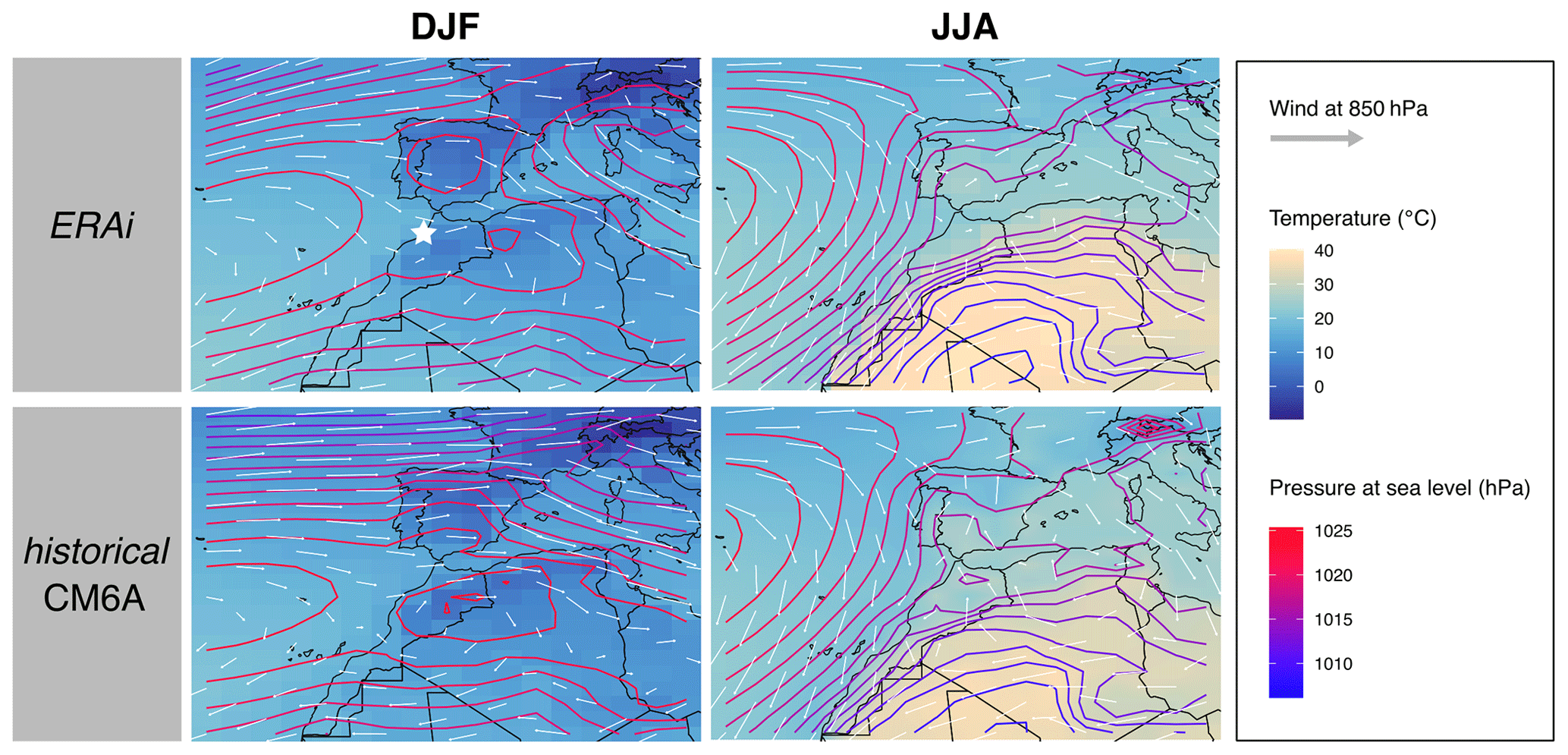
Figure 1 Maps of mean temperature (color; unit: ^∘C), wind speed and direction at 850 hPa (represented by arrows; length is proportional to wind speed) and sea level pressure (isolines; unit: hPa) for two seasons (DJF and JJA) as represented by (top) the global atmospheric reanalysis ERA-Interim (ERAi; Berrisford et al., 2011) and (bottom) the historical simulations of IPSL–CM6–LR models in the region of EH. Data are averaged on 30 seasonal cycles (1980–2009). EH cave location is represented by a star in the upper left panel. DJF: December, January, February (winter); JJA: June, July, August (summer).

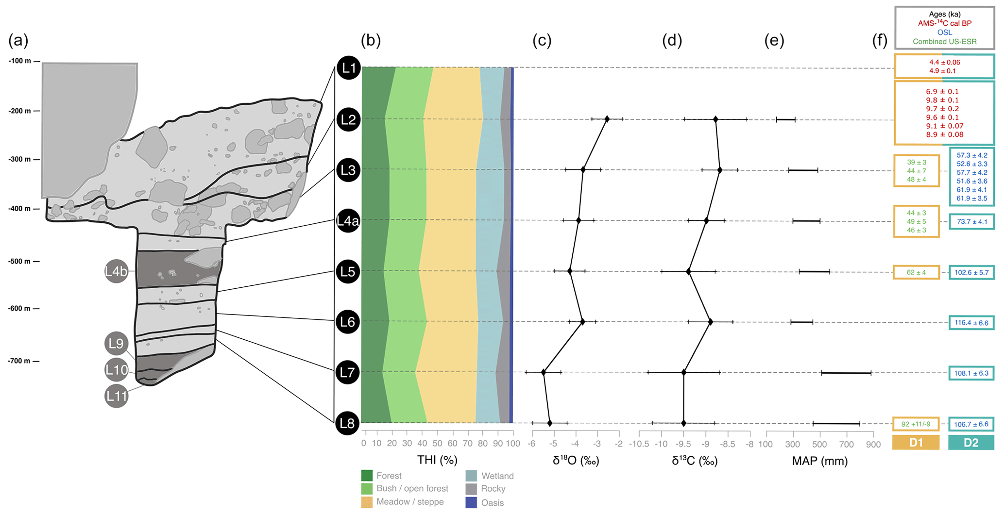
Figure 2 Summary diagram displaying stratigraphy, paleoenvironmental proxies and the two dating hypotheses of El Harhoura 2 (EH). (a) Stratigraphy of EH; unused layers are in dark gray. (b) Relative percentage of THI values (adapted from Stoetzel et al., 2014, and Jeffrey, 2016). (c) Mean δ¹⁸O values in Meriones teeth (from Jeffrey, 2016). (d) Mean δ¹³C values in Meriones teeth (from Jeffrey, 2016). (e) Mean annual precipitation (MAP; from Jeffrey, 2016). (f) Dating hypotheses D1 (brown) and D2 (blue) for the different layers of EH (Nespoulet and El Hajraoui, 2012; Jacobs et al., 2012; Janati-Idrissi et al., 2012; Ben Arous et al., 2020b, a; Marquer et al., 2022).

2.1.2 Chronostratigraphy and dating hypotheses

EH displays a high-resolution stratigraphy, and its layers have revealed an impressive taxonomic richness and delivered an significant amount of large and small vertebrate remains (Michel et al., 2009; Stoetzel et al., 2011, 2012b). Its stratigraphy is currently divided into 11 layers (Fig. 2a) (each layer is abbreviated as “L” followed by the number of the layer; for consistency the present is referred to as “L0”). Among these layers eight are well studied and considered in this study. All of these eight layers have been dated (Ben Arous et al., 2020b). Three different methods were used: AMS-¹⁴C (Nespoulet and El Hajraoui, 2012; Marquer et al., 2022), OSL (Jacobs et al., 2012) and combined US–ESR (Janati-Idrissi et al., 2012; Ben Arous et al., 2020a). AMS-¹⁴C is the most reliable dating method of the three and is used for recent layers (L1 and L2). However, for older layers beyond the reach of AMS-¹⁴C (L3, L4a, L5, L6, L7 and L8), OSL and combined US–ESR methods are used. However, when applied to the same layer, these two methods present discrepancies. This is the case, for example, of L5 dated at ∼ 60 ka by combined US–ESR and at ∼ 100 ka by OSL (Fig. 2f). In addition, when two consecutive layers are dated with these different methods, dates can be inconsistent with the relative position of the layers in the stratigraphy, as is the case for L8 dated at ∼ 90 ka using combined US–ESR and L7 at ∼ 110 ka using OSL (Fig. 2f). To overcome this issue, we choose to set two separate dating hypotheses (D's) of the stratigraphic sequence. In the following, D1 refers to the chronological sequence based on AMS-¹⁴C and combined US–ESR dates, and D2 refers to the sequence based on AMS-¹⁴C and OSL dates. The D's are presented in Fig. 2f.

2.1.3 Paleoenvironmental variables

Paleoenvironments at EH have been inferred based on two different kinds of proxies: species presence and stable-light-isotope composition. Regarding species presence, paleoenvironments are reconstructed using the taxonomic habitat index (THI). The THI is a paleoecological index which allows one to reconstruct the paleolandscape based on the species composition of the community (Stoetzel, 2009; Stoetzel et al., 2011, 2014). Each species is associated with its preferred habitat based on the assumption that species' ecological preferences were the same in the past as they are today. From that a qualitative composition of the paleolandscape is deduced, expressed as a percentage. Data are from Stoetzel et al. (2014) and are presented in Fig. 2b. Note that the oasis habitat was not considered because its percentage of presence does not vary over the EH sequence.

Isotope-based inferences are from Meriones teeth. They provide information about the diet and the environment of studied individuals (Longinelli and Selmo, 2003; Navarro et al., 2004; Royer et al., 2013). Two isotopic fractions are considered: δ¹⁸O and δ¹³C. Plants consumed by small mammals are sensitive to environmental conditions, which shows up in their δ¹³C and δ¹⁸O values. Because of that, they are good indirect indicators of aridity, seasonal variation and vegetal cover (Longinelli and Selmo, 2003; Blumenthal et al., 2017; Blumenthal, 2019). We used δ¹⁸O and δ¹³C means, minimums and maximums and reconstructed mean annual precipitation (MAP) computed from δ¹⁸O from Jeffrey (2016). Data are presented in Fig. 2c, d and e.

2.2 Paleoclimate simulations

2.2.1 Climate model and experiments

We ran a new set of paleoclimate simulations covering the Late Pleistocene to mid-Holocene period using the model LMDZOR6A (Hourdin et al., 2020). This model is the atmosphere–land surface component of the IPSL–CM6A–LR coupled model (Boucher et al., 2020) that has been used to run the CMIP6 ensemble of past, present and future coupled climate simulations (Eyring et al., 2016), including the mid-Holocene (Braconnot et al., 2021), last interglacial (Sicard et al., 2022; Otto-Bliesner et al., 2021) and Pliocene (Haywood et al., 2016) periods. It has an atmospheric resolution of 144 points in longitude, 143 points in latitude and 79 vertical levels (144 × 143 × L79). Compared to previous IPSL model versions it has a finer spatial and vertical resolution and an improved representation of atmospheric and land surface processes. In addition, when the model is run for present-day conditions (with sea surface temperature prescribed to the monthly climatology of the observed Atmospheric Model Intercomparison Project (AMIP) sea surface temperature (SST) fields; Boucher et al., 2020, 2018), the simulated climatology of temperature and precipitation over the region is consistent with observations (Figs. 1 and 3). The simulated annual mean cycle of surface air temperature and precipitation matches quite well with the observed one, despite an overestimation of summer temperature and slight 0–1-month shift in the seasonal cycle of precipitation (Fig. 3).

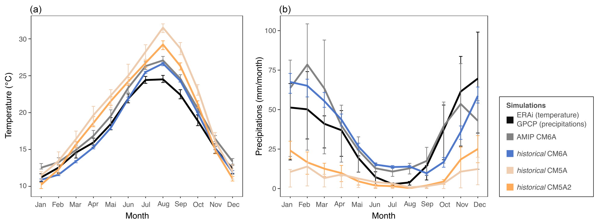
Figure 3 Annual mean cycle of mean temperature (a; unit: C^∘) and precipitation (b; unit: millimeters per month) from the ERAi and Global Precipitation Climatology Project (GPCP) reanalyzed data, the AMIP CM6A simulations (atmosphere only), and historical coupled simulations of IPSL–CM5A–LR, IPSL–CM5A2–LR and IPSL–CM6–LR models. Data are averaged on 30 seasonal cycles (1980–2009) and on the four grid cells containing EH cave. Error bars are estimated from interannual variation over the averaged 30 years and visualized by quartiles. As a reference for current climate we used monthly data from the global atmospheric reanalysis ERA-Interim for monthly mean temperature (Berrisford et al., 2011) and from the GPCP v2.3 (Global Precipitation Climatology Project) for monthly mean precipitation (Adler et al., 2018).

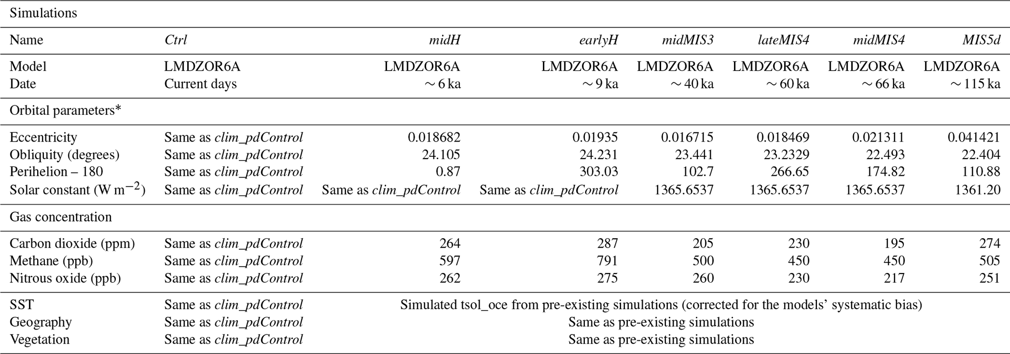
We produced a total of six paleoclimate simulations with the LMDZOR6A model for the key periods of the EH sequence: midH (for the mid-Holocene period), earlyH (for the early Holocene period), midMIS3 (for the mid-MIS3 period), lateMIS4 (for the late MIS4 period), midMIS4 (for the mid-MIS4 period) and MIS5d (for the MIS5d period). The different simulations differ in terms of prescribed Earth orbital parameters, atmospheric trace gas composition, ice-sheet configuration and SST in order to represent the climate conditions of the different periods (see Table 2 for details). For this we make use of pre-existing paleoclimate and control simulations that have been run in the last 10 years with different versions of the IPSL model (Marti et al., 2010; Dufresne et al., 2013; Boucher et al., 2020) (details are available in Table 1). For all these simulations the vernal equinox is prescribed to occur on 21 March at noon (GMT), following the Paleoclimate Modeling Intercomparison Project (PMIP; Kageyama et al., 2018) recommendations.

Table 1 Pre-existing coupled simulations from the IPSL repository.

Table 2 Forcing and boundary conditions of the simulations produced in this study.

^* The term “orbital parameters” refers to variations in the eccentricity of the Earth and longitude of perihelion as well as changes in its axial inclination (obliquity).

We also ran a control simulation Ctrl (see Table 2 for details), representative of the present-day climate. The SST boundary conditions used in Ctrl correspond to the mean annual cycle of the SST estimated from current observations used for the AMIP (Boucher et al., 2018) and repeated in time. This Ctrl simulation will be considered to be the reference for the current climate in our ensemble of new atmospheric simulations.

Unfortunately, simulated paleoclimate SSTs are not directly comparable because they were performed using different versions of the IPSL model (Table 1). This is due to the fact that the various versions of the model are characterized by different physical representations, resolutions and tuning. In particular, these different model versions show different present-day SST biases when compared to observations (Fig. 4). When these paleoclimate SSTs simulated using different model versions are used as boundary conditions in simulations run with LMDZOR6A (instead of the AMIP SST field), they translate to different representations of the seasonal cycle of surface air temperature and precipitation at EH (Fig. 3). The magnitude of the seasonal cycle is overestimated, and precipitation is underestimated, with almost no seasonality when IPSL–CM5A or IPSL–CM5A2 control SST is used as boundary condition. The differences that can be attributed exclusively to the differences in the SST biases are significant and may deteriorate the simulation of other variables of interest, thus complicating the intercomparison between our new LMDZOR6A simulations. Indeed, the differences between these simulations for the periods of interest at EH could then result from the difference in bias between the various versions of the model rather than representing significant climate differences between periods. In order to produce a homogeneous set of simulations we thus apply a correction to the SST fields (described below). The objective is to correct differences due to model versions while preserving differences related to climate variation between past periods. These corrected SST fields are used as the prescribed paleoclimatic SST boundary conditions in our new ensemble of LMDZOR6A simulations.

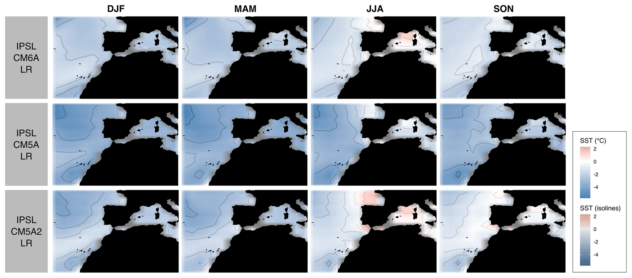
Figure 4 SST biases of IPSL–CM5A–LR, IPSL–CM5A2–LR and IPSL–CM6A–LR relative to AMIP's SST (issued from current observations) (color and isolines; unit: ^∘C) for the four seasons. The seasons are DJF (December, January, February; winter), MAM (March, April, May; spring), JJA (June, July, August; summer) and SON (September, October, November; autumn).

2.2.2 Sea surface boundary conditions

We correct the simulated SST of each coupled simulation for the systematic bias of the model. This is done by removing the SST bias corresponding to the model version used. In other words, corrected SSTs were obtained according to the formula

$$\begin{array}{}\text{(1)}& \mathrm{SSTcor}=\mathrm{SSTsim}+(\mathrm{SSTamip}-\mathrm{SSTmod}),\end{array}$$

where SSTsim is the SST from the coupled simulation; SSTamip is the AMIP SST; SSTmod is the SST of the model version for current days; and SSTcor is the corrected SST, which is used as a boundary condition in our new LMDZOR6A simulations. The underlying assumption in this correction scheme is that the mean annual SST bias cycle, i.e., SSTmod − SSTamip for each, is stationary in time. Note also that boundary condition files of pre-existing (coupled) simulations were interpolated on a 143 × 144 × L79 grid to be compatible with the grid of LMDZOR6A. The corrections are applied to daily SST values of the modern climate so that the changes in season from the orbital parameters are properly accounted for in the new daily SST imposed as a boundary condition given the way the vernal equinox is prescribed in the model.

Configuration details for the new set of simulations are summarized in Table 2. The length of all these new simulations is 50 years, which is long enough given the fact that LMDZOR6A is an atmospheric model. In the following annual mean cycles are estimated from the last 30 years of each LMDZOR6A simulation.

2.2.3 A subset of key paleoclimate variables

To characterize the large-scale climate over the area, we worked on the mean annual cycle of the four grid cells containing EH. From simulations Ctrl, midH, earlyH, midMIS3, lateMIS4, midMIS4 and MIS5d we extracted nine output variables. We choose to focus on variables that are likely to directly or indirectly influence the landscape and/or the biotic environment. Based on a review of the ecological literature, we selected tsol (temperature at surface, C^∘) (Gillooly et al., 2001; Yom-Tov and Geffen, 2006; Ebrahimi-Khusfi et al., 2020), precip (precipitation, millimeters per month) (Yom-Tov and Geffen, 2006; Alhajeri and Steppan, 2016; Ebrahimi-Khusfi et al., 2020), qsurf (specific humidity, kg kg⁻¹) (Hovenden et al., 2012; Alhajeri and Steppan, 2016), w10m (wind speed at 10 m, m s⁻¹) (McNeil, 1991; Tanner et al., 1991; Chapman et al., 2011; Pellegrino et al., 2013), sols (solar radiation at surface, W m⁻²) (Monteith, 1972; Fyllas et al., 2017), drysoil_frac (fraction of visibly dry soil, %) (Paz et al., 2015) and humtot (total soil moisture, kg m⁻²) (Paz et al., 2015). Two additional variables are computed: the diurnal temperature range tsol_ampl_day (C^∘; Alhajeri and Steppan, 2016) computed from tsol_max (daily maximum temperature) and tsol_min (daily minimum temperature) as tsol_max − tsol_min and the hydric stress hyd_stress (mm d⁻¹; Martínez-Blancas and Martorell, 2020) computed from evapot (potential evaporation) and evap (evaporation) as evapot − evap.

We explore variation in annual means (mean values of the variables) and annual standard deviations (amplitude of seasonal variation). The means and standard deviations are computed on the annual mean cycle estimated from the last 30 years of each LMDZOR6A simulation; thus they represent, respectively, the annual mean and the seasonal amplitude of the variable. In all analyses, climate variables are standardized between periods.

Potential biases related to calendar effect (the change in length of seasons and months between periods; Bartlein and Shafer, 2019; Joussaume and Braconnot, 1997) were considered and discounted in the statistical analyses by characterizing the annual mean cycles by their annual means and standard deviations. Indeed, these metrics are only slightly, if at all, affected by the calendar effect, in particular when they are properly weighted by the number of days in the months (estimated using the modern or a celestial calendar). This choice is made to keep the physical consistency between the different variables that nonlinearly depend on moisture and temperature.

The association of paleoclimate simulations with the stratigraphic layers of EH is based on age proximity. This step is performed for both D1 and D2 (the D's presented in Sect. 2.1.2). As a result, we obtain two hypothetical paleoclimate sequences corresponding to EH sequence.

In order to easily visualize the climate proximity and differences between EH layers we used a principal component analysis (Jolliffe and Cadima, 2016). This analysis allows one to find new uncorrelated variables that successively maximize variance (the principal components). They are computed from the eigenvectors and eigenvalues of the covariance–correlation matrix (correlation matrix in our case, as all the variables are standardized). Then, the data can be visualized along the leading principal components, which maximizes the amount of information displayed. It allows us to visualize EH layers along the two main axes of variance in climate data, resulting in the proximity between stratigraphic layers (points) in the plot representing the proximity between the climate of the layers. The principal component analyses are performed on the annual mean and standard deviations (seasonal amplitude) of climate variables.

2.3 Consistency analyses

To test the consistency between the paleoclimate simulations and paleoenvironmental inferences that have been made from the content of the EH site we use two kinds of analyses: two-block partial least squares (2B-pls) and pairwise correlation tests. For these analyses, the climate variables are the principal components provided by the principal component analysis described above. Working on principal components instead of original variables allows us to take into account the interrelationships between climatic variables as well as to separately consider the uncorrelated axes of variance (which are the principal components), which may display different covariation with paleoenvironmental indicators. The different paleoenvironmental proxies considered are δ¹⁸O and δ¹³C means, minimums and maximums and MAP as well as percentages of represented habitats indicated by the THI.

The 2B-pls tests the global covariance between climate variables and paleoenvironmental variables. This multivariate method explores patterns of covariation between two sets of variables, i.e., two blocks (Sampson et al., 1989; Streissguth et al., 1993). Axes of maximum covariance between the two blocks are generated, thus reducing data dimensionality. A coefficient (r-PLS) is computed and represents the strength of covariation. The r-PLS is in the range of (0, 1). The closer the r-PLS is to 1, the stronger the covariation. The p values indicating the statistical significance of r-PLS are calculated based on 1000 permutations against the null hypothesis (absence of covariation between the two sets of variables). Then, to refine our results, we perform pairwise correlation tests.

3 Results

3.1 Simulated climate changes

Changes in atmospheric circulation and pressure over the sequence are presented in Fig. 5, and plots of monthly precipitation and temperatures for the region of EH are available in Fig. 6. The proximity between the climate of each period and current climate is shown on similarity maps in Fig. 7. We did not account for the calendar effect in these graphs; they are only there to illustrate the major differences between the periods that are not affected by it.

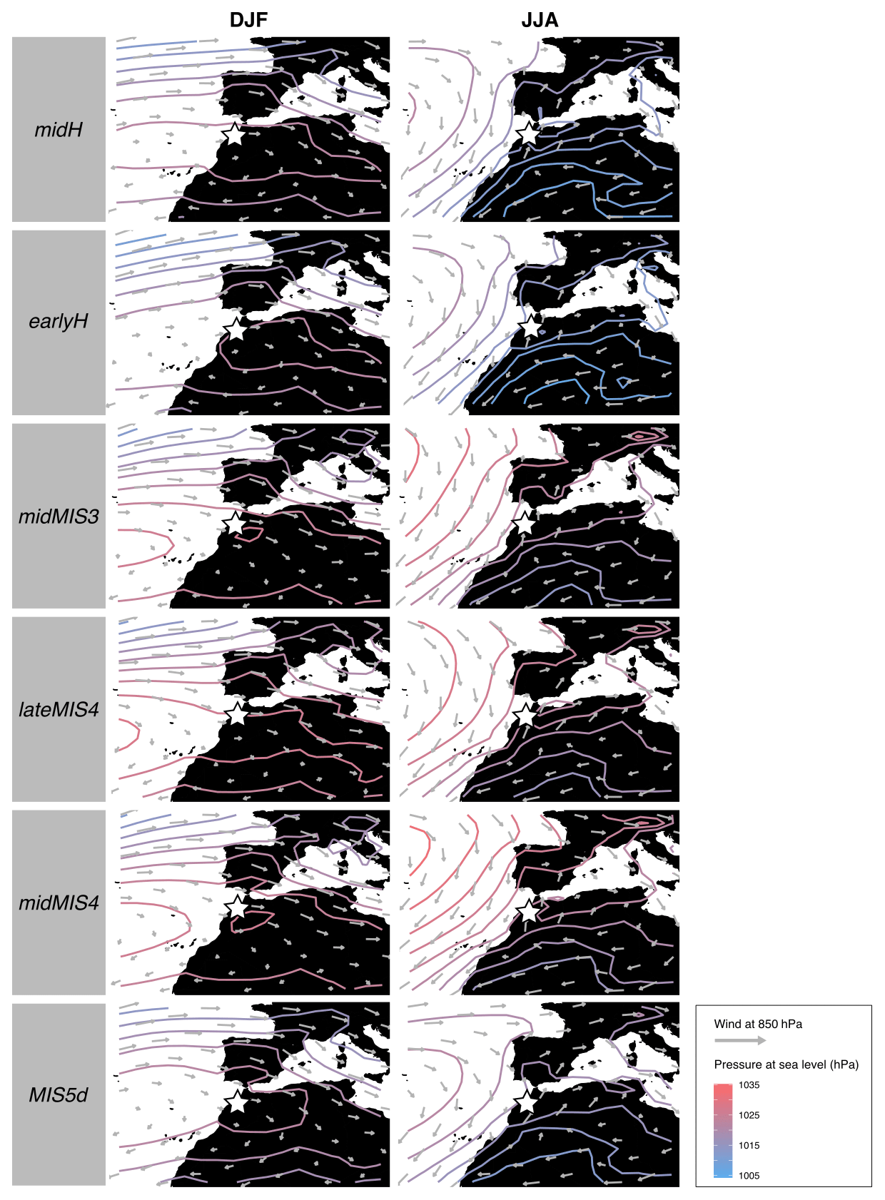
Figure 5 Maps of wind speed and direction at 850 hPa (represented by arrows; length is proportional to wind speed) and corrected pressure at sea level (isolines; unit: hPa) for two seasons (DJF and JJA) from midH, earlyH, midMIS3, lateMIS4, midMIS4 and MIS5d. EH cave location is represented by a white star. DJF: December, January, February (winter); JJA: June, July, August (summer).

The atmospheric circulation over the region differs between winter and summer. Winter is marked by a meridional pressure gradient and dominated by a zonal flow from west to east. In summer, the pressure gradient is more horizontally oriented, with the establishment of a depression on the North African continent and the northward drift of high pressures in the Atlantic Ocean (Fig. 5). All over the sequence, these features shift slightly, especially between lateMIS4, midMIS4 and midMIS3 (period from ∼ 66 to ∼ 40 ka) and Ctrl, midH and earlyH (period from ∼ 9 ka until today) (Figs. 5 and 7), with the exception of MIS5d (∼ 115 ka), the conditions of which are relatively close to current ones, as shown in Fig. 7. There are also significant changes in the magnitude of the seasonal temperature variation from June to October and in the seasonal precipitation variation from October to May between these two major periods (Fig. 6).

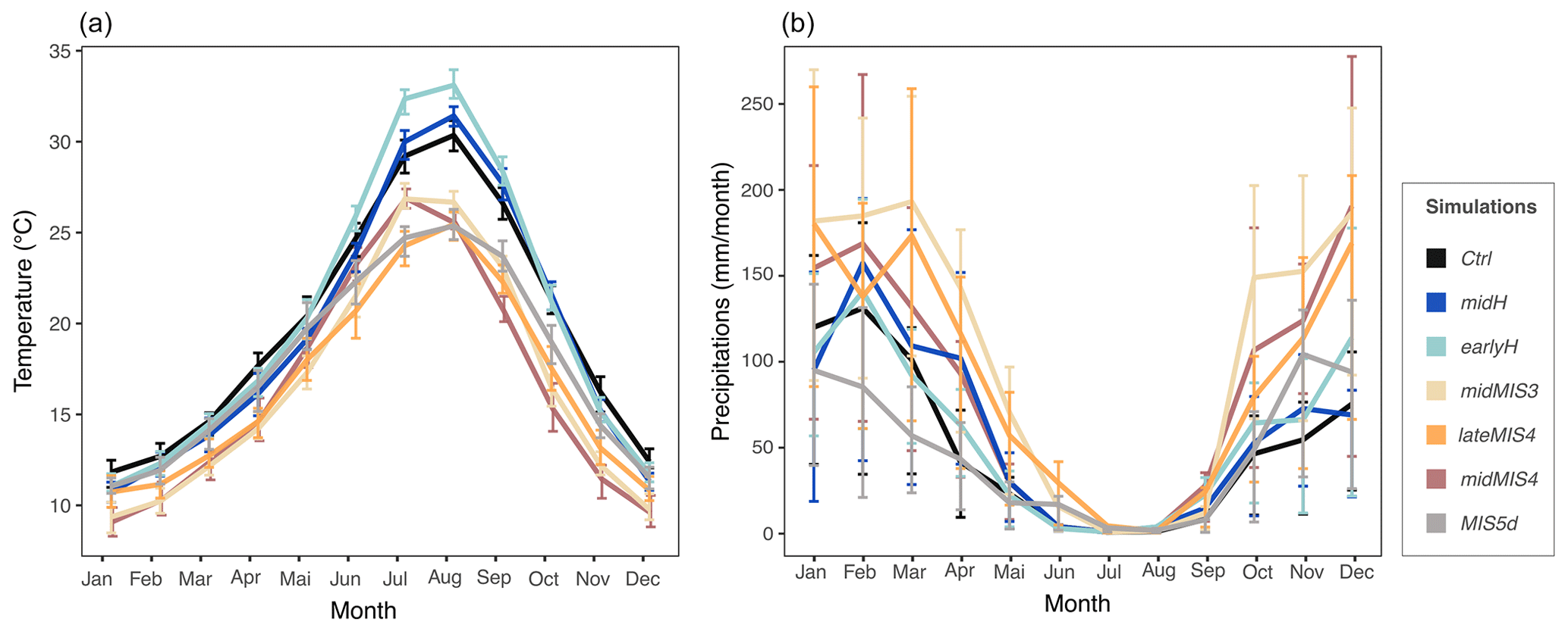
Figure 6 Mean annual cycle of temperature (a; unit: ^∘C) and precipitation (b; unit: millimeters per month). Data are averaged on 30 seasonal cycles and on the four grid cells containing EH cave. Error bars are estimated from interannual variation over the averaged 30 years and visualized by quartiles.

From ∼ 115 ka (MIS5d) until ∼ 40 ka (midMIS3), the climate was colder than today. From ∼ 66 ka (midMIS4) to ∼ 40 ka (midMIS3), there is also more precipitation in winter (Fig. 6). These conditions share similarities with what can be found at slightly higher latitudes today (Fig. 7), which is consistent with the pressure along the North African (and Moroccan) coast (Fig. 5). In ∼ 115 ka (MIS5d), conditions are also cold, but as dry as in the Holocene (Fig. 5). They are not related to changes in the atmosphere circulation (Fig. 5) but rather to changes in insolation, with current analogs limited to North Africa (Fig. 7). Starting from ∼ 9 ka (earlyH) the seasonal temperature variation is enhanced. Conditions in winter and spring are similar to the current climate (Fig. 7), but with a warmer autumn and a much warmer summer (Fig. 6). At ∼ 6 ka (midH), climate conditions are close to today (Fig. 7), but with a slightly more significant seasonal temperature variation (Fig. 6).

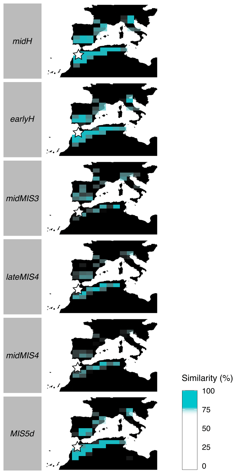
Figure 7 Maps presenting the similarity between past climates in EH and current climate in the area. For each cell in the Ctrl simulation, we computed the Euclidean distance between the climate variables (means and standard deviations) associated with the cell and the climate variables of the four cells containing EH of each past period. Blue cells indicate localities where current climate is more than 75 % similar to past climate in EH (blue scale indicates the degree of similarity). EH cave location is represented by a white star.

3.2 Consistency between paleoclimate simulations and paleoenvironmental inferences

3.2.1 Association of paleoclimate simulations and stratigraphic layers

The two hypothetical paleoclimate sequences corresponding, respectively, to D1 and D2 are presented in Fig. 8. The two principal components analyses are shown in Fig. 9. To visualize how climate variables structure the climate space of these two principal component analyses, biplots are available in Supplement Fig. S2.

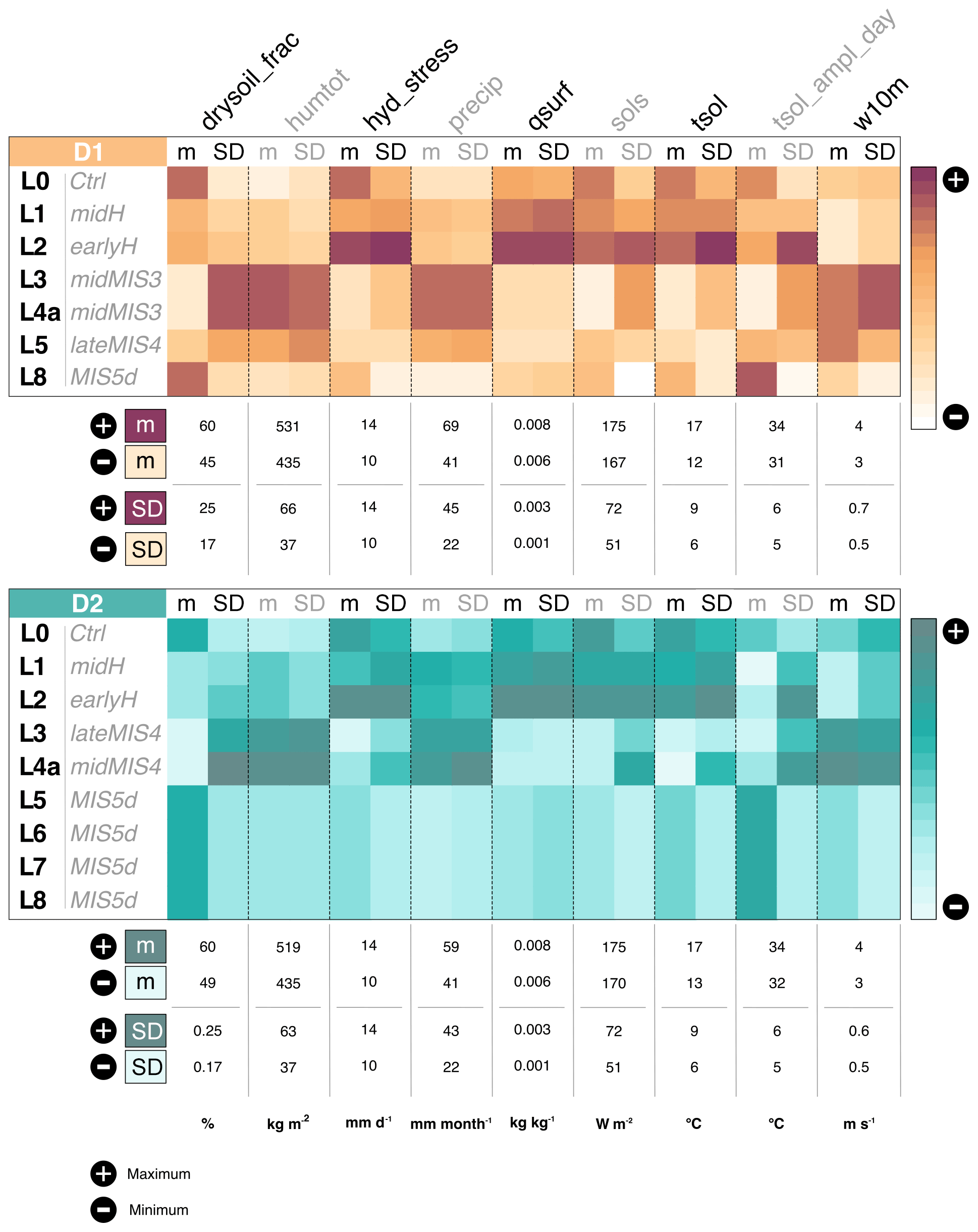
Figure 8 Climate variation over the EH sequence according to D1 (dating hypothesis 1; in brown) and D2 (dating hypothesis 2; in blue). The color scales reflect the intensity of the variables: an intense color (brown for D1, blue for D2) indicates a maximum, while a clear (white) color indicates a minimum. Maximum (+) and minimum (−) refer to the range of values explored by each variables with their original unit across simulations. “L” is the abbreviation for layer, “m” is mean, and “SD” is standard deviation.

Based on D1, our results indicate four major climate transitions (Fig. 8). The first occurs between L8 and L5. In L5 the climate is wetter and colder, with more precipitation, more soil humidity, increased wind speed, less hydric stress and a smaller portion of dry soil. Humidity, precipitation and wind speed also show a significant seasonal variability. The second transition, less marked, is between L5 and L4a. Climate in L4a is rather similar to the climate in L5, but precipitation and humidity have increased. Seasonal variation are globally more pronounced. The third transition is between L3 and L2. The climate changes drastically between these two periods, with hotter and drier conditions in L2 corresponding to the end of the last deglaciation. Temperature, solar radiation, water stress and soil dryness all increase, coupled with a decrease in precipitation, soil moisture and wind speed. All these changes are consistent with aridification or desertification from L2. Surprisingly, however, specific humidity is enhanced, which is partly consistent with the decrease in precipitation and wind speed at this coastal location and is concomitant with large changes in the atmospheric circulation patterns over this region from L2 (Fig. 5). The last climatic transition is more subtle and occurs between L1 and L0. The environment in L0 seems closer to the one in L8, with more seasonal variability in temperature, solar radiation and water stress (Fig. 8).

Overall, there is an alternation of two main climate types. This partition is confirmed by the principal component analysis shown in Fig. 9. The first principal component explains 65.85 % of the observed variance (of the standardized variables) and splits the layers of EH into two climate regimes. The first regroups L3, L4a and L5 and is defined by humid and windy conditions, with a high seasonal variability. The second includes L0, L1, L2 and L8 and is characterized by hot and dry conditions. The second axis, explaining 30.28 % of the variability, divides the latter group into two subgroups: L1 and L2, with high seasonal variability, and L0 and L8, with a lower seasonal variability.

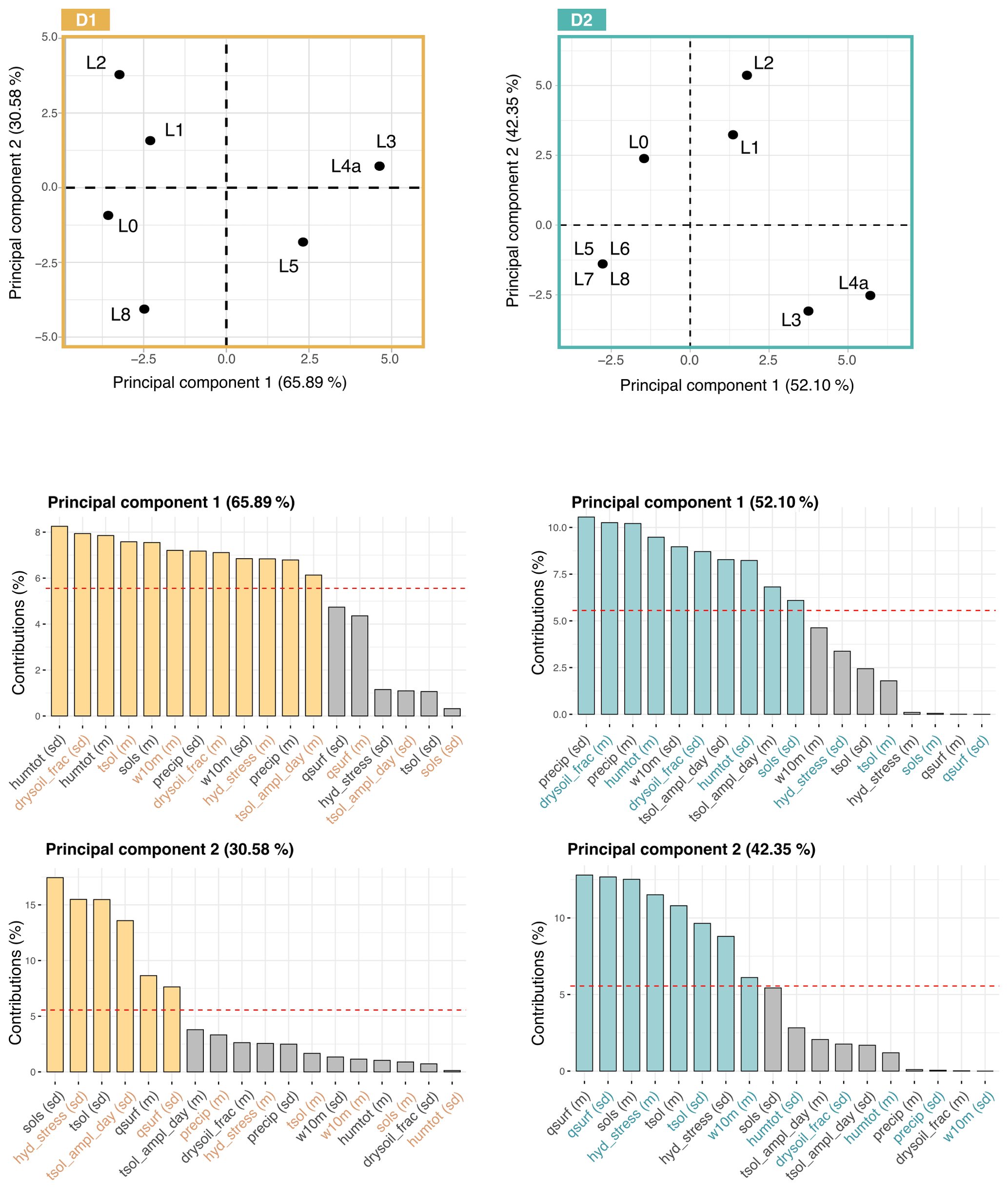
Figure 9 Principal component analyses performed on climate variables according to D1 (dating hypothesis 1; in brown) and D2 (dating hypothesis 2; in blue). The axes represent the two leading principal components (along which data are visualized), and the numbers in parentheses are the percentage of variance carried by each axis. The bar plots below each graph present the contributions of the (standardized) climate variables to the two leading principal components (variables above the horizontal red line contribute significantly). “L” is the abbreviation for layer. To better distinguish the variable names, they are presented with two colors (black and the color corresponding to the dating hypothesis).

Regarding D2, we observe three significant and abrupt climatic transitions (Fig. 8). The first happened between L5 and L4a. In L4a, the climate is much windier, and temperatures are colder, with a substantial increase in diurnal temperature range. Precipitation and soil moisture increase significantly, while hydric stress decreases. The climate also presents an overall higher seasonal variability. These tendencies persist in L3. The second transition is between L3 and L2. The soil is drier, and the hydric stress increases greatly as well as solar radiation and temperature. Precipitation and soil moisture are less important. Conditions in L1 are close to those in L2, but a bit colder with a less marked water stress. The last climate transition, smoother than the previous ones, occurs between L1 and L0 and is mainly marked by a global decrease in seasonal variation.

Results associated with D2 suggest that three types of climate succeeded one another at EH. The first group is composed of L8, L7, L6 and L5; the second of L3 and L4a; and the third of L2, L1 and L0. As for D1, this partition is supported by the principal component analysis presented in Fig. 9. The first principal component, which explains 52.10 % of the observed variance, separates the group containing L8, L7, L6 and L5 from the one composed of L3 and L4a. The second principal component, explaining 42.35 % of the observed variance, separates the group of L2, L1 and L0 from others. L8, L7, L6 and L5 are characterized by a hot and dry climate and a low seasonal variation. L3 and L4a are defined by a wet and windy climate, with significant precipitation and high seasonal variability. Finally, L2, L1 and L0 present a hot environment associated with a significant water stress.

3.2.2 Consistency analyses

Results of 2B-pls and pairwise correlations between climate and paleoenvironmental variables are presented in Fig. 10. Regarding D1, no significant covariation is found between THI values and climate variables. However, 2B-pls shows that there is a statistically significant covariation between isotope data and all climate variables and between isotope data and the second principal component (climate variables contributing to the second principal component are detailed in Fig. 9). Specifically, this second principal component is positively correlated with δ¹⁸O mean, maximum and minimum values and δ¹³C maximum values. Conversely, D2 presents neither a statistically significant result for 2B-pls nor correlations, meaning that for D2 paleoclimate inferences and paleoenvironmental proxies are not consistent.

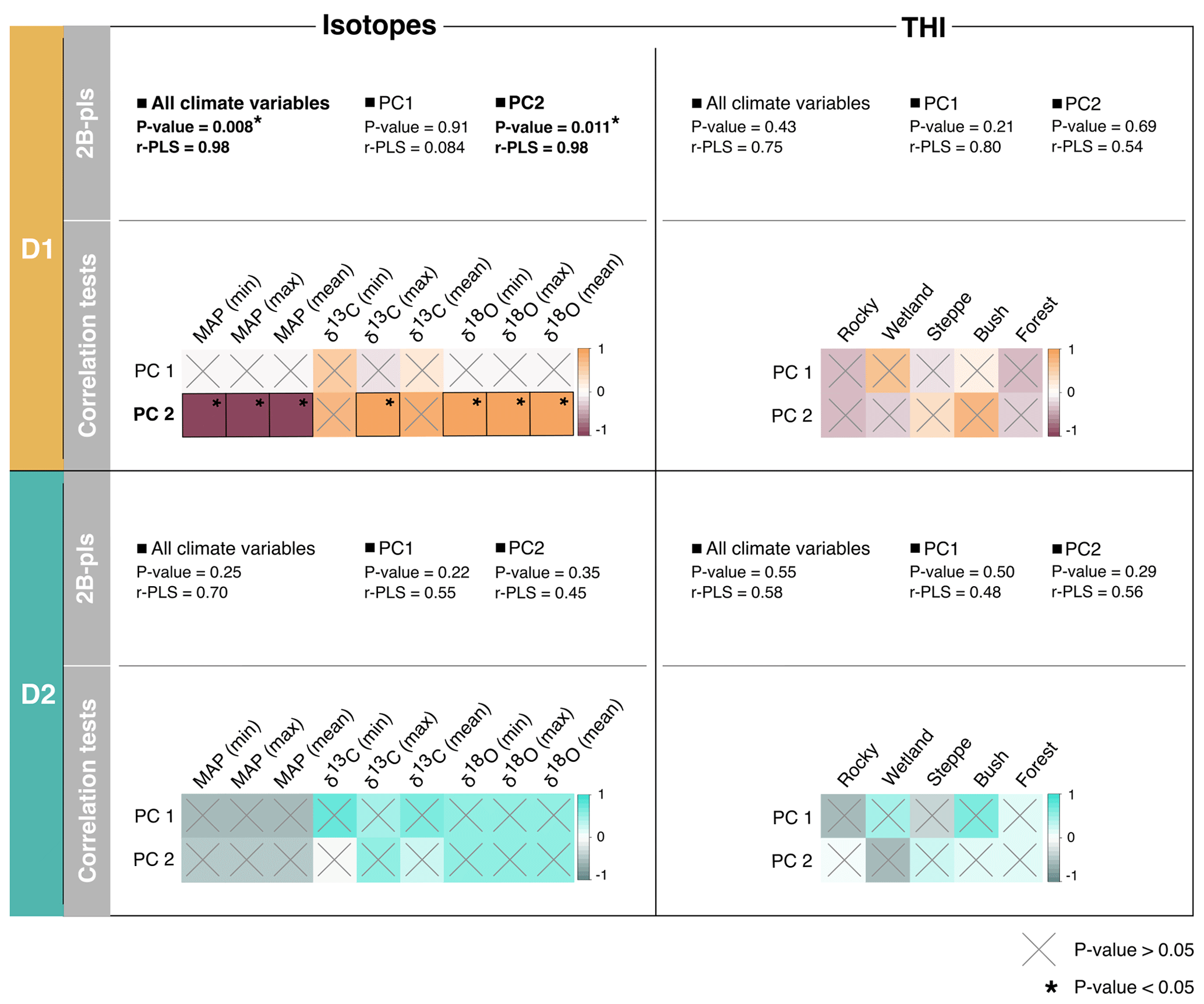
Figure 10 Results of the 2B-pls and correlation tests performed between isotopes (Jeffrey, 2016) and THI values (Stoetzel et al., 2014) and climate variables according to D1 (dating hypothesis 1; in brown) and D2 (dating hypothesis 2; in blue). Statistically significant results (p value < 0.05) are indicated by ^*. Regarding correlation tests, crosses indicate cases where correlation is not significant (p value > 0.05), and colors represent the strength of the correlations. For isotopes: δ¹⁸O and δ¹³C values are from Meriones teeth (from Jeffrey, 2016), and MAP is the mean annual precipitation (from Jeffrey, 2016). For THI: forest, bush, steppe, wetland and rocky refer to relative percentage of the representation of environmental types according to the THI (from Stoetzel et al., 2014, and Jeffrey, 2016).

4 Discussion

Despite the differences in scale and resolution between climate and paleoenvironmental data, we find statistically significant and meaningful results. The climate changes considered seem to be large enough for a consistency to be detected between the climate and environmental data. First, we discuss the paleoclimate changes described by simulations over the period and the underlying dynamical processes. Then, we address the contribution of climate simulations to the discussion of chronological and paleoenvironmental discrepancies of EH.

4.1 Paleoclimate variation and underlying forcings

Paleoclimate simulations allow us to discuss several significant climate changes at EH over the Late Pleistocene to mid-Holocene period. These paleoclimate variations may result from the mixed influence of global and regional dynamical processes.

Radiation-related variables (as sols, tsol or tsol_ampl_day) seem to largely depend on global processes related to large-scale climate changes. They clearly separate interglacial climate (Ctrl, midH, earlyH) from glacial climate (midMIS3, lateMIS4, midMIS4, MIS5d). The warm/cold differences between these two periods are due to the size of the ice sheet and variation in gas concentration. For example, mean insolation and temperature significantly increase in the early Holocene relative to other periods, along with increasing greenhouse gas concentrations and the retreating ice sheet. Also, obliquity and precession of the Earth orbit increase at this period relative to others, along with the amplitude of the seasonal variability in insolation and temperature. Note that MIS5d is a peak of the glacial sub-stag,e where conditions were quite mild, which explains the proximity of its climate to the current one.

The variation in the humidity-related variables (as precip, hydric_stress or drysoil_frac) seems to be mainly explained by a translation of the regional atmospheric circulation processes over the sequence. For example, mean precipitation and soil moisture are higher from mid-MIS4 to mid-MIS3. At this time, the wet and cold westerly winds descend further south and blow across the area of EH. This is explained by the position of the Azores High: the magnitude of the high pressures creates a stronger pressure gradient, thus favoring a stronger zonal circulation, which brings cooler and more humid air to the North African coast. Therefore, for this region, the atmospheric circulation effect and changes in moisture advection over the region have a significant impact on whether a warmer climate would lead to increased moisture content and precipitation.

4.2 Paleoclimate simulations and chronostratigraphy

The climate sequence differs significantly depending on the D it is based on. Based on D1, there is an alternation of semi-arid and temperate climates. The climate succession based on D2 is quite different, with the presence of three main climate types and rapid transitions between them. The climate sequences based on D1 and D2 are not equally congruent with paleoenvironmental proxies from the literature. Indeed, several statistically significant correlations and covariation are found between the climate sequence based on D1 and the paleoenvironmental inferences, while none are found for the one based on D2. Thus, our results suggest that, with respect to EH, combined US–ESR dating may be more reliable than OSL dating. As the OSL dating process relies on quartz grains and because their chronology and origin are difficult to establish in the context of karstic coastal caves (as discussed in Ben Arous et al., 2020a), OSL ages might have been overestimated (i.e., the age of the layers may be younger than that estimated by OSL). Moreover, OSL dates can in some cases be internally inconsistent, meaning that they can have a number of reversals. For instance, it is known that water content influences the determinations. Considering the location of the cave on the coastline, inundations related to rising sea level or very high tides may have occurred.

4.3 Paleoclimate simulations and paleoenvironmental inferences

Because the climate sequence based on D1 is the only one displaying significant results, we focus on it in the following discussion. Isotope fractions are mainly correlated to seasonal variation in water stress (hyd_stress), insolation (sols) and temperature (tsol, tsol_ampl_day). This result is expected because δ¹⁸O is an indicator of aridity (Longinelli and Selmo, 2003; Blumenthal et al., 2017; Blumenthal, 2019), and δ¹³C is related to seasonal variation in temperature and water stress (O'Leary, 1988; Lin, 2013; Smiley et al., 2016). In contrast to isotopes, the THI is not related to climate variation. It is not completely surprising, as THI is a qualitative estimate of the global environment provided by the whole microvertebrate community. It is therefore very dependent on the species included in the estimate. Conversely, isotopes reveal quantitative fluctuations in particular variables that are temperature- and precipitation-related provided by a limited number of individuals of a single species. Thus, they do not deliver information at the same resolution, nor do they estimate it using the same approaches.

Another explanation of the improved correlations between climate and isotope fractions may be that biologically derived proxies (as the THI) are more complex functions of physical drivers than the isotope signal. Isotopes directly reflect to the magnitude of seasonal variation in insolation, water stress, temperature and diurnal temperature range because these variables condition the presence of essential elements for plants' survival (e.g., sunlight, water in the soil). Thus, they are directly related to the type of vegetation. On the other hand, the THI relies on the ecological preferences of species. Altogether, the variables of the THI give information about the proportion of biomes (e.g., forest, bush, steppe), and thus the spatial distribution and density of the vegetation. Consequently, its relationship to climate is more indirect than for isotopes.

The large climatic variation observed over the sequence allows us to discuss paleoenvironmental inconsistencies between isotopes and THI at EH. The two major ones concern L5 and L7. In both cases, isotope surveys and MAP from Jeffrey (2016) indicate more humid conditions with more significant precipitation than in other layers. In contrast, the THI as well as the presence of the steppic species Jaculus cf. orientalis (often used as an indicator of particularly arid conditions) and the scarcity of aquatic species supports a drier climate than in other layers (Stoetzel, 2009; Stoetzel et al., 2014). Large mammals would also support this last hypothesis, with an increase in the representation of gazelles and alcelaphines and a decrease in the representation of bovines in both layers (Stoetzel et al., 2012a, 2014). Unfortunately, no combined US–ESR ages are available for L7 to date. Considering that climate conditions associated with L8 display less precipitation than currently, we could hypothesize a similar climate for L7. In that case, this would support inferences from species presence. Nevertheless, we cannot exclude the possibility that a microclimatic event could have induced particular climatic conditions in L7. Concerning L5, the climate described by the sequence based on D1 agrees with isotope surveys (Jeffrey, 2016). These conclusions are supported by the abundance of Crocidura russula, a shrew species associated with Mediterranean climates (Cornette et al., 2015). In addition, Jaculus cf. orientalis can also be considered to be an indicator of more continental conditions, such as the distance from the coastline, rather than a marker of arid environments.

An important difference is noticed between the climate sequence and the THI in L1. The paleoclimate simulation indicates a quite dry climate relative to other layers, in contradiction with the composition of small and large mammal communities that suggests an expansion of forests and wetlands (Stoetzel et al., 2014). This difference could be explained by the location of EH: the cave is located at the interface of varied climate influences, as described previously. Because global climate models describe general climate characteristics, a local climate phenomenon could have generated a wetter environment in the surroundings of EH.

4.4 Perspectives and limitations of the interdisciplinary approach

The interdisciplinary approach between archeology and paleoclimatology presented in this study opens new avenues for testing the consistency between paleoclimatic simulations and paleoenvironmental reconstructions in different regions. The contextualization of archeological and paleontological sites could greatly benefit from this approach. Environmental and/or chronological uncertainties such as the ones encountered at EH are unfortunately common in archeology, since the observed differences depend primarily on the method-specific biases, not especially on the site. However, while the results of this approach are promising in the case of EH, extending it to other sites is only possible under certain conditions. (1) The concerned site must have been well studied, and data on the chronology of the sequence must be available from different methods. (2) Paleoenvironmental inferences must also be available, and preferably from different sources. (3) The stratigraphic sequence must be composed of a sufficient number of levels to allow the application of statistical methods. (4) Fully coupled climate simulations of the periods of interest must be available, otherwise their complete production would represent a considerable amount of work.

While not all sites meet these criteria, a large number of them have been heavily studied and could benefit from our approach, such as other Moroccan sites (Ben Arous et al., 2020b) or sites from the cradle of humankind (Hanon et al., 2019; Pickering et al., 2019). Moreover, with the development of more powerful statistical tools, this approach could even be extended to other sites with less referenced context. Paleoclimate simulations such as the ensemble we used here are becoming more common and distributed so that their availability should be less of a concern in the coming years. The most crucial point is to encourage collaboration between the fields of archeology and paleoclimatology, as expertise in both disciplines is needed to properly combine the different types of information.

5 Conclusions

Considering paleoclimate simulations and paleoenvironmental inferences together allows us to provide new insights into the chronostratigraphy and paleoenvironmental reconstruction of El Harhoura 2 cave. We find that the climate sequence based on combined US–ESR ages is more consistent with paleoenvironmental inferences than the climate sequence based on OSL ages. We also show that, overall, isotope-based paleoenvironmental inferences are more congruent with the paleoclimate sequence than species-based inferences. But, above all, we highlight the difference in scale between the information provided by each of these paleoenvironmental proxies. This study demonstrates that the combination of different sources of environmental data and climate simulations has great potential for refining the paleoenvironmental and chronological context of archeological and paleontological sites. Even so, its applicability to periods marked by less significant climate changes remains to be tested. Our approach may concern a limited number of well-studied sites; however with more powerful statistical tools, it could be extended to other sites whose context is less referenced.