No changes in overall AMOC strength in interglacial PMIP4 time slices

The Atlantic Meridional Overturning Circulation (AMOC) is a key mechanism of poleward heat transport and an important part of the global climate system. How it responded to past changes in forcing, such as those experienced during Quaternary interglacials, is an intriguing and open question. Previous modelling studies suggest an enhanced AMOC in the mid-Holocene compared to the preindustrial period. In earlier simulations from the Palaeoclimate Modelling Intercomparison Project (PMIP), this arose from feedbacks between sea ice and AMOC changes, which were dependent on resolution. Here we present an initial analysis of recently available PMIP4 simulations for three experiments representing different interglacial conditions – one 127 000 years ago within the Last Interglacial (127 ka, called lig127k), one in the middle of the Holocene (midHolocene, 6 ka), and a preindustrial control simulation (piControl, 1850 CE). Both lig127k and midHolocene have altered orbital configurations compared to piControl. The ensemble mean of the PMIP4 models shows the strength of the AMOC does not markedly change between the midHolocene and piControl experiments or between the lig127k and piControl experiments. Therefore, it appears orbital forcing itself does not alter the overall AMOC. We further investigate the coherency of the forced response in AMOC across the two interglacials, along with the strength of the signal, using eight PMIP4 models which performed both interglacial experiments. Only two models show a stronger change with the stronger forcing, but those models disagree on the direction of the change. We propose that the strong signals in these two models are caused by a combination of forcing and the internal variability. After investigating the AMOC changes in the interglacials, we further explored the impact of AMOC on the climate system, especially on the changes in the simulated surface temperature and precipitation. After identifying the AMOC's fingerprint on the surface temperature and rainfall, we demonstrate that only a small percentage of the simulated surface climate changes could be attributed to the AMOC. Proxy records of sedimentary $\mathrm{Pa}/\mathrm{Th}$ ratio during the two interglacial periods both show a similar AMOC strength compared to the preindustrial, which fits nicely with the simulated results. Although the overall AMOC strength shows minimal changes, future work is required to explore whether this occurs through compensating variations in the different components of AMOC (such as Iceland–Scotland overflow water). This line of evidence cautions against interpreting reconstructions of past interglacial climate as being driven by AMOC, outside of abrupt events.

1 Introduction

The Atlantic Meridional Overturning Circulation (AMOC) is a large system of ocean currents involving differences in the temperature and salinity between the water in the tropics and the North Atlantic Ocean (Rahmstorf, 2006). The upper cell of the AMOC consists of warm and salty northward surface flow (the North Atlantic warm current, down to roughly 1200 m depth), along with colder and deep southward return flow (the North Atlantic Deep Water, 1500–4000 m depth). The lower cell of the AMOC is the northward flow of dense Antarctic Bottom Water (AABW) formed in the Southern Ocean (Buckley and Marshall, 2016). The AMOC acts as a heat pump at the high latitudes as the meridional transportation brings warm water to the colder sub-polar and polar regions (Chen and Tung, 2018) then further modifies the climate in northern Europe and the east coast of North America (Găinuşă-Bogdan et al., 2020). It is responsible for producing about half of the global ocean's deep waters, sourced from the northern North Atlantic (Petit et al., 2021).

Since the AMOC plays a vital role in air–sea interactions, along with its ability to transport and redistribute heat and its effect as a carbon sink in the Northern Hemisphere (Gruber et al., 2002), studying the evolution of the AMOC strength in the past is of great importance for us. It helps us identify the mechanisms which lead to the AMOC changes (Buckley and Marshall, 2016) and make projections for the future climate. Comparison of the AMOC changes between different geological eras can provide us with a better understanding of the roles of the external forcing in the AMOC strength variations. In addition, past AMOC variations suggest that the distribution of surface heat and freshwater flux can affect the location of deep water formation and result in transient changes in the AMOC (Kuhlbrodt et al., 2007).

Our study focuses on investigating the AMOC changes during the two interglacials: the Holocene (11.5 ka–1950 CE) and Last Interglacial (130–115 ka). Two time slice experiments, the midHolocene (representing 6 ka) and the lig127k (representing 127 ka), have been defined by the Palaeoclimate Modelling Intercomparison Project Phase 4 (PMIP4) (Kageyama et al., 2018); 6 ka was chosen as the warmest point during the Holocene thermal maximum according to existing surface temperature reconstructions (Joussaume and Braconnot, 1997), although this is being re-evaluated at present (Marsicek et al., 2018). The midHolocene experiment is one of the entry cards (Kageyama et al., 2018) for the PMIP4 component of the current phase of the Coupled Model Intercomparison Project (CMIP6); 127 ka is chosen as it represents the peak boreal warmth in the Last Interglacial (Capron et al., 2017), and it has been identified as a period of high interest, due to its higher average global temperature and sea level (Capron et al., 2017; Otto-Bliesner et al., 2017). In the context of PMIP4, the focus lies on changes in insolation arising from the differences in Earth's orbit, while the greenhouse gas (GHG) concentrations were similar to that in the piControl experiment, and the continental configuration (ice-sheet distribution and elevations, land–sea mask, continental topography, and oceanic bathymetry) was prescribed as the same as in piControl (Otto-Bliesner et al., 2017).

During the two interglacial periods, the orbital parameters are prescribed according to Berger and Loutre (1991). Eccentricity, the deviation of the Earth's orbit from a perfect circle, was larger (more elliptic) than that during the preindustrial period, especially for lig127k. Meanwhile, perihelion, the closest point in the orbit to the sun, occurred much closer to the boreal summer solstice in lig127k. Obliquity, the tilt of the Earth's axis, was also higher during these two warm periods (Otto-Bliesner et al., 2017). This leads to a positive Northern Hemisphere summer insolation anomaly at both 127 and 6 ka, compared to preindustrial, while the difference in annual incoming insolation at the top of the atmosphere between the two periods is marginal (see Fig. 3b of Otto-Bliesner et al., 2017, for the seasonal distribution of insolation). Due to the model differences in the internal model calendar and the impact of eccentricity and precession (the orientation of Earth's rotational axis) on the length of the seasons, the date of the vernal equinox must be fixed in all simulations to 21 March (Joussaume and Braconnot, 1997; Otto-Bliesner et al., 2017). More detail on the forcings and boundary conditions for the lig127k and midHolocene experiments can be found in Otto-Bliesner et al. (2017) and in Eyring et al. (2016) for the piControl experiment. Based on the experimental set-up, midHolocene and lig127k, when the seasonal insolation is the strongest forcing, are two reasonable periods to study whether or not the changes in orbital forcing have altered the overall AMOC strength in the two past interglacials compared to the piControl experiment.

After introducing the methods used in this study (Sect. 2), we first analyse the behaviour of AMOC during the Quaternary interglacials in individual PMIP4 models in Sect. 3, and then we explore the AMOC variations during the past two interglacials based on the model ensemble mean, which are shown in Sect. 3.1. In Sect. 3.2, as the seasonal changes in incoming solar radiation amplified in lig127k compared to midHolocene, we investigated further to see whether the simulated response shows similar amplification in these individual models or not. Meanwhile, we also devised a series of tests that must be passed for a forced response and also try to identify the causes for the changes in AMOC that we see in individual models. Furthermore, since we have identified that the AMOC changes could leave a fingerprint on the surface temperature and precipitation variation in midHolocene, as well as in piControl, regressions of surface conditions against AMOC have been computed for each simulation run for both midHolocene and piControl, and they are shown in Sect. 4. Based on the computed AMOC's fingerprint on the surface temperature and precipitation in individual models, we also show in this section that the percentage of simulated surface temperature changes that could be explained by AMOC changes is only minor. After investigating the changes in AMOC and the role of AMOC in the climate system in PMIP4 simulations, comparisons with proxy reconstructions for the Holocene and the Last Interglacial are discussed in Sect. 5.

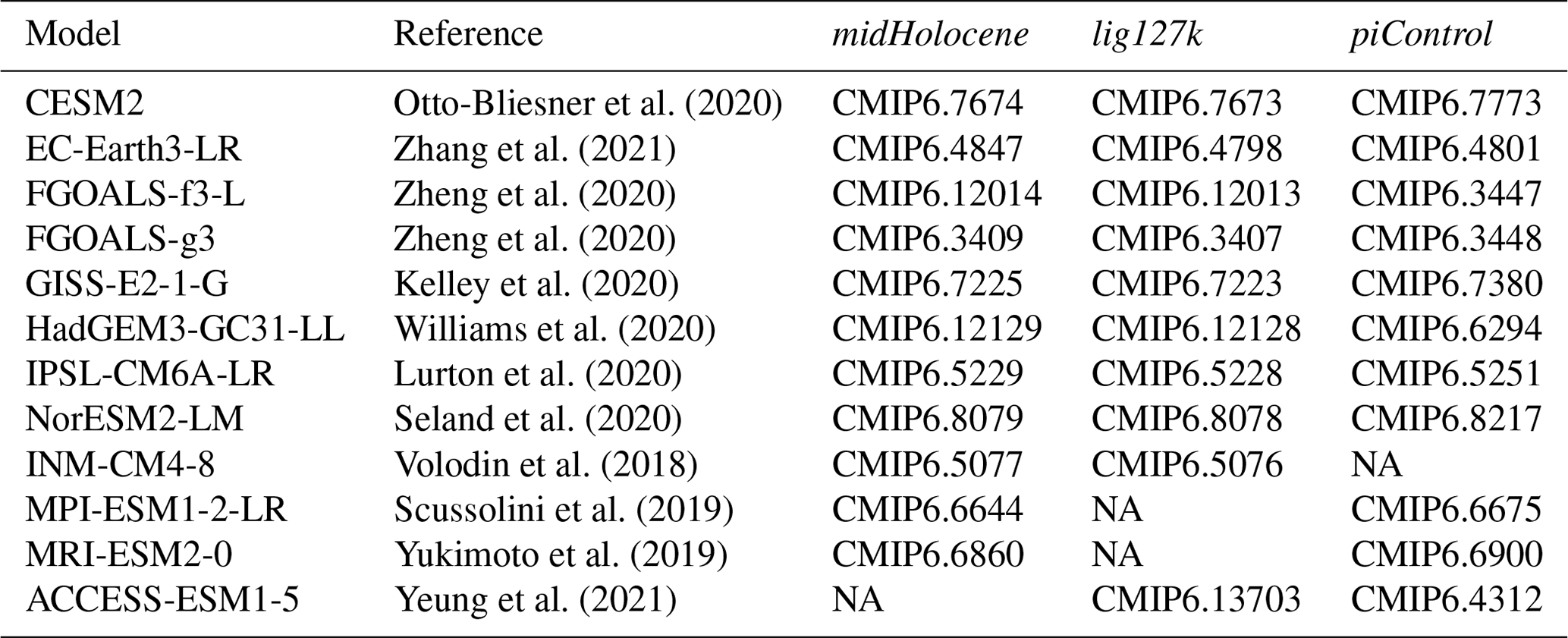
Otto-Bliesner et al. (2020)Zhang et al. (2021)Zheng et al. (2020)Zheng et al. (2020)Kelley et al. (2020)Williams et al. (2020)Lurton et al. (2020)Seland et al. (2020)Volodin et al. (2018)Scussolini et al. (2019)Yukimoto et al. (2019)Yeung et al. (2021)

Table 1 Model simulation length (after spin-up, in years) and the AMOC strength at 30^∘ N (in sverdrups, also with the standard deviation). The data from FGOALS-f3 L used for the preindustrial conditions actually come from the historical simulation for years 1850 to 1899, as the necessary data are not available (NA) for the piControl simulation.

2 Methods

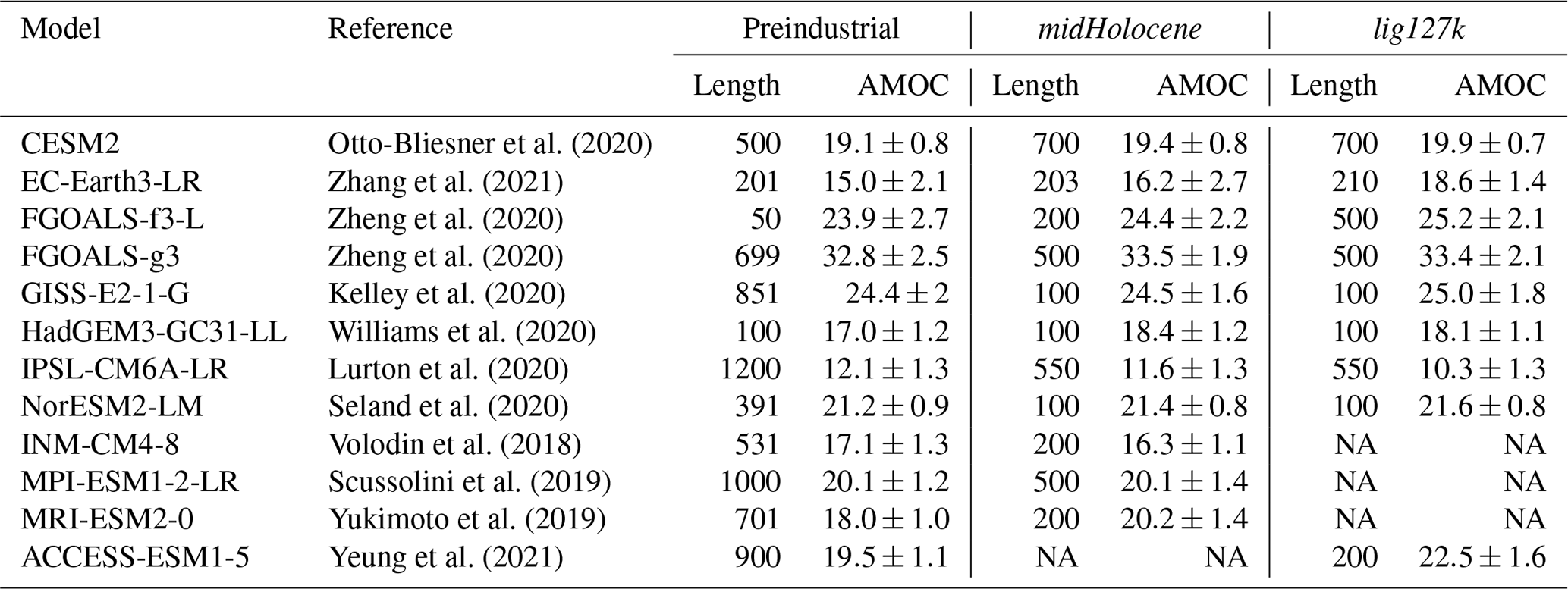
To be included in this study, a model must have performed an experiment following the protocol for either midHolocene or lig127k as laid out by Otto-Bliesner et al. (2017) and then archived the output of this experiment with the Earth System Grid Federation. Twelve CMIP6 models have provided the necessary output of zonal-mean ocean meridional overturning mass streamfunction (called “msftmz” or “msftmyz” depending on the grid used) to undertake our analysis. Of these, eight models performed both interglacial experiments. Details of the individual models are shown in Table 1.

The AMOC intensity is computed using a modified version of the Climate Variability Diagnostic Package (CVDP; Phillips et al., 2014; Danabasoglu et al., 2012). Rather than using principal component analysis to define the AMOC (Danabasoglu et al., 2012), the maximum overturning streamfunction at 30^∘ N is used (Zhao et al., 2022). Patterns of surface climate anomalies associated with AMOC variations are computed by the CVDP via linear regression (more details below), with the ability to determine precipitation patterns added by Zhao et al. (2022).

The maximum of the annual-mean meridional mass overturning streamfunction below 500 m at 30^∘ N (and additionally at 50^∘ N) is used to measure the AMOC strength. If the latitudes of, say, 35 or 55^∘ N had been selected instead, the impacts on the results would be subtle (Brierley et al., 2020) and would be unlikely to alter our conclusions. Observational mooring arrays exist at 26^∘ N (RAPID-MOCHA, since 2004) (Rayner et al., 2011; Frajka-Williams et al., 2019) and at 53–60^∘ N (OSNAP section, since 2014) (Lozier et al., 2019).

All models are regridded onto a common 1^∘ latitude grid with 61 depth levels ranging between 0–6000 m in the ocean to compute ensemble averages. All simulations are given equal weighting when calculating ensemble means.

A fingerprint of the AMOC on wider climate is computed separately for each simulation. The fingerprints are obtained by linearly regressing temperature and precipitation anomalies at each grid box over the globe onto AMOC strength at 30^∘ N, using the equation: $\mathit{\delta }T=\mathit{\alpha }\mathit{\delta }{\mathrm{\Psi }}_{\text{30N}}+c$, where δ indicates a detrended anomaly within a simulation, T is the temperature (at the grid point), Ψ is the maximum overturning streamfunction at 30^∘ N in the Atlantic, α is the fingerprint coefficient, and c is a constant. A 15-month low-pass Lanczos filter is applied to the AMOC time series prior to computing the regression. Precipitation fingerprints are computed using percentage variations, rather than absolute rainfall anomalies. The maximum contribution of local surface temperature changes that could be explained by AMOC changes is then estimated by comparing simulated changes to the AMOC change multiplied by the regression coefficient (averaged between the interglacial and preindustrial simulations) ($\mathrm{\Delta }{T}_{\mathrm{\Psi }}/\mathrm{\Delta }T$).

3 Simulated AMOC during midHolocene and lig127k

The first-order determinant on the AMOC strength is the model used for the simulation (Table 1). Figure 1a clearly shows that the piControl AMOC strength at 30^∘ N is highest in FGOALS-g3, with it ranging between 12–25 sverdrups (Sv) in the rest of the models. The highest simulated AMOC strength is more than twice that of the lowest one, even excluding FGOALS-g3. The dashed green and pink horizontal lines in Fig. 1a show the average value from observational arrays. The observed AMOC strength at 26^∘ N (17 Sv; Frajka-Williams et al., 2019) is stronger than that at 53–60^∘ N from the OSNAP section (Lozier et al., 2019; Srokosz et al., 2012). The stronger sub-tropical strength feature is generally replicated by models, except for ACCESS-ESM1-5 and FGOALS-g3 (Fig. 1a).

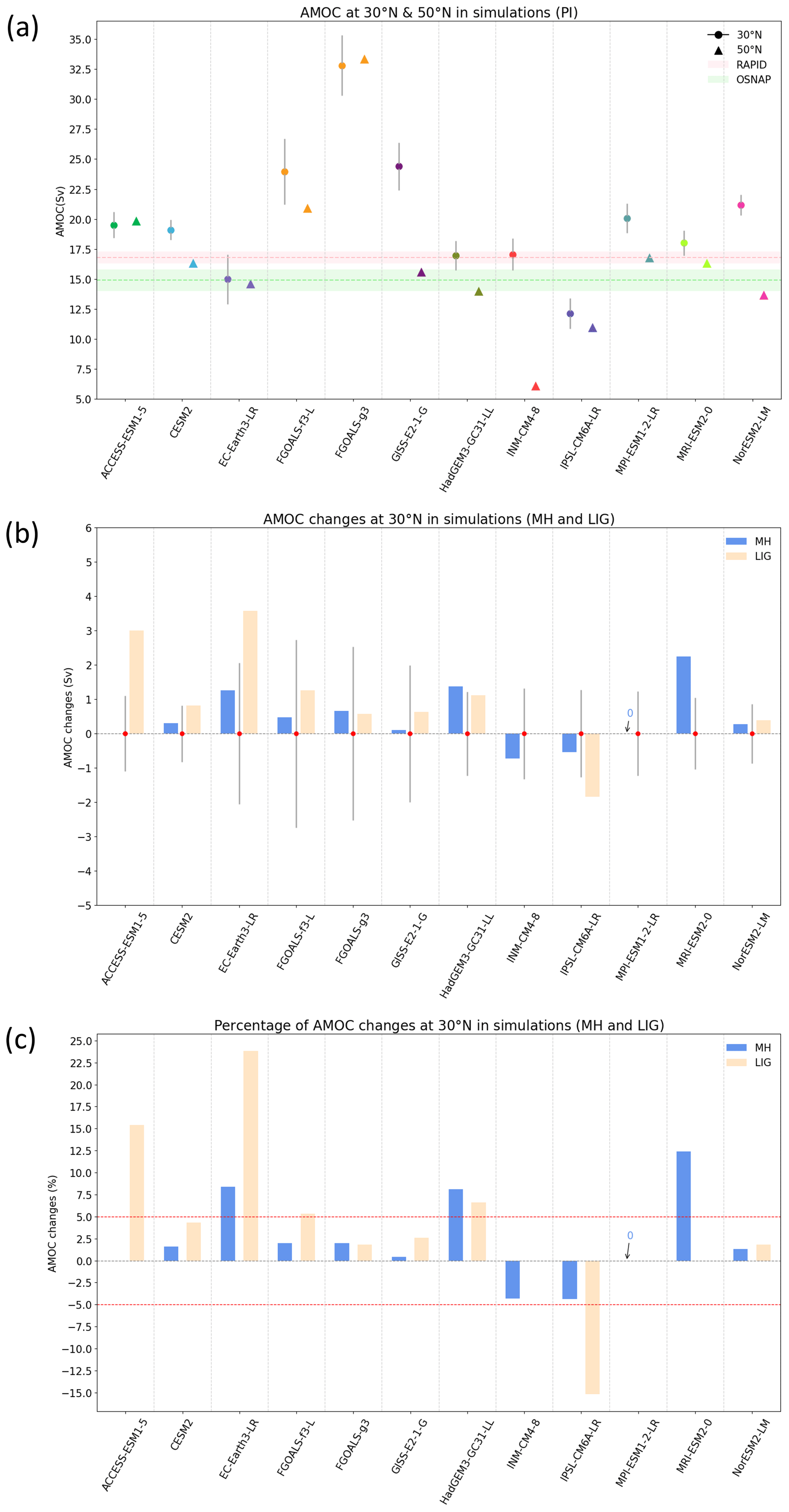
Figure 1 Maximum AMOC strength and AMOC changes. (a) Maximum AMOC strength at 30^∘ N (circles, with error bars indicating 1 standard deviation) and 50^∘ N (triangles) in preindustrial control simulations. Observational estimates of the present-day AMOC strength are shown from both the RAPID-MOCHA array (26^∘ N; Rayner et al., 2011; Frajka-Williams et al., 2019) and the OSNAP section (53–60^∘ N; Lozier et al., 2019). (b) Absolute AMOC changes at 30^∘ N in the midHolocene and lig127k experiments (with respect to piControl). The error bars between the two histograms of each model show the magnitude of the internal variability (1 standard deviation) of each model's piControl experiment. (c) Percentage of AMOC changes at 30^∘ N in the midHolocene and lig127k experiments (with respect to piControl). Data within the ±5 % range indicate no obvious AMOC changes (Brierley et al., 2020). The number 0 is annotated in (b) and (c) as the MPI-ESM1-2-LR model does not show any AMOC changes between midHolocene and piControl (see Table 1).

The large spread in the simulated AMOC strength seen in the piControl experiment raises questions about whether the models can accurately simulate changes in AMOC (Eyring et al., 2021). The spread is an unfortunate feature of both the wider CMIP6 and CMIP5 ensembles (e.g. Xie et al., 2022). Disappointingly the uncertainty in modern-day oceanographic observations is such that few of the simulations can be categorically ruled out (Weijer et al., 2020). The piControl experiment represents an earlier time than that of the observations, and AMOC is known to have changed between them (Thornalley et al., 2018; Caesar et al., 2018). However, the changes in AMOC seen during the historical simulations (Gong et al., 2022) are relatively small compared to the differences between the models and observations, meaning that the consequences of the temporal offset are not important.

The extremely low value in the IPSL-CM6A-LR model is mainly caused by the inaccurate representation for the overflow waters or deep western boundary current (DWBC) and biases in the precipitation in the North Atlantic Ocean, which are challenging to resolve in climate models (Boucher et al., 2020). In some models, the lack of overflow parameterisations which commonly occur in low-resolution models (Danabasoglu et al., 2014) could be another reason for the slightly underestimated simulated AMOC strength. The AMOC strength in the FGOALS-g3 model in both sub-tropical and sub-polar regions is very high, even compared to its predecessor FGOALS-g2 (Li et al., 2020). These can be attributed to the excessive deep convection in the Irminger Sea, Labrador Sea, and Nordic Seas, despite a mixed layer depth similar to observations (Li et al., 2020).

The interannual variability in the AMOC is also model-dependent (Table 1) and generally does not alter much between the various experiments. EC-Earth3-LR and the two models by FGOALS are the exceptions, but they do not provide a coherent message about the response to increasing orbital forcing. Therefore, we consider these to be different samples from the same underlying distribution (Latif et al., 2022).

The absolute AMOC changes in the midHolocene and lig127k experiments (with respect to piControl) are compared to the magnitude of the internal variability (1 standard deviation) of each model's piControl experiment (Fig. 1b). The magnitude of the simulated AMOC changes in midHolocene are within the range of the model's internal variability for all the models, except for HadGEM-GC31-LL and MRI-ESM2-0. The extent of AMOC changes in lig127k is generally larger, with three different models (ACCESS-ESM1-5, EC-Earth3-LR, and IPSL-CM6A-LR) showing changes that are larger than their internal variability.

Given the large spread in AMOC strength in piControl, it is also worth looking at the relative changes in AMOC seen in the midHolocene and lig127k experiments (Fig. 1c). Changes within the ±5 % range (dashed red horizontal lines) have previously been considered to represent no substantial AMOC changes (Brierley et al., 2020). The majority of models do not demonstrate a substantial change in AMOC strength under the midHolocene experiment at 30 or at 50^∘ N (Table 1, Fig. 1c). Brierley et al. (2020) state that these findings are consistent with the palaeo-reconstructions for the mid-Holocene, something discussed further in Sect. 5. Similar results are seen for lig127k (Fig. 1c), although five models do have AMOC strength changes exceeding 5 % of the piControl strength. The extent of deviations in lig127k is generally larger than that seen in midHolocene.

3.1 Ensemble mean AMOC changes

To explore the spatial patterns of changes in the AMOC structure in past warm interglacials, we compute PMIP4 ensemble mean AMOC changes (Fig. 2). The overlaid contours display the model-averaged AMOC pattern in the piControl experiment to help place these changes in context. The two plots do not reveal a substantial change in the AMOC strength at the location where the maximum AMOC occurs (35–40^∘ N, 1000 m). There is a slight increase of about 0.4–0.8 Sv in the maximum AMOC strength in midHolocene, growing to 1.0–1.4 Sv in lig127k. There is a slight intensification of the midHolocene model-averaged AMOC strength at depth (below 2000 m, with the largest changes up to 1.0–1.2 Sv at 2500 m in the sub-tropics). The lig127k experiments do not show such a focus of their intensification at depth, with the largest changes occurring in the top 500 m (Fig. 2b). An overall stronger AMOC in lig127k is confined at the low mid-latitudes, as the AMOC strength becomes weaker in the sub-polar and polar regions (north of 55^∘ N). Since the midHolocene and lig127k ensembles contain some different models, we additionally analyse the pattern of AMOC changes between midHolocene and lig127k only using the models which have AMOC data in both of the periods (eight models in total). This demonstrates that the different increases in shallow (top 1000 m at low mid-latitudes) (lig127k; Fig. 2b) and deep (below 2000 m at 0–60^∘ N) (midHolocene; Fig. 2a) branches are not an artefact of the additional models (Fig. 2c).

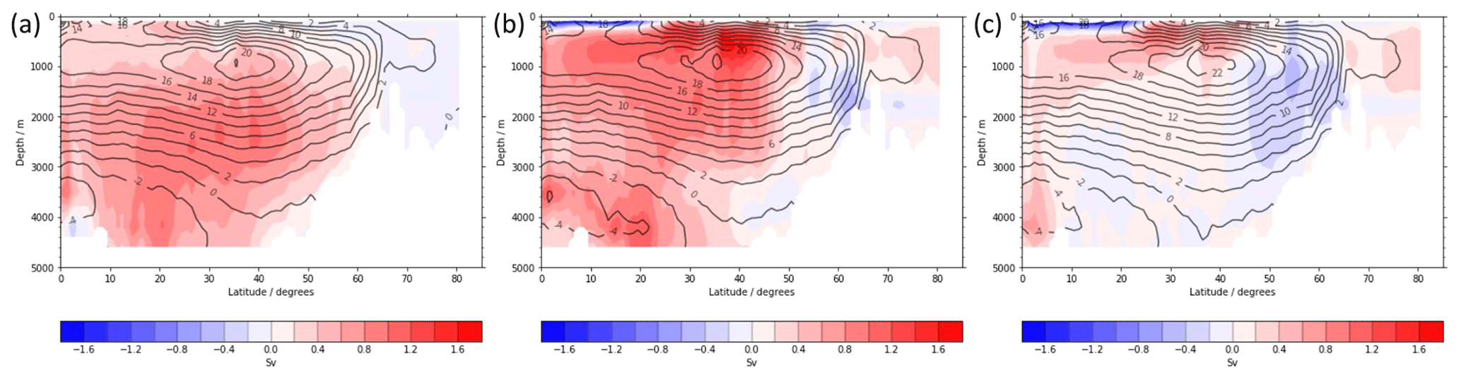
Figure 2 Ensemble, annual-mean AMOC spatial structure changes in PMIP4. (a) Ensemble mean AMOC changes between the 11 PMIP4 models that have performed the midHolocene and piControl experiments. (b) Ensemble mean AMOC changes between lig127k and piControl (consisting of nine models). (c) Ensemble mean AMOC changes between the lig127k and midHolocene experiments (eight models). Overlaid black contours show model-averaged AMOC strength in the respective piControl simulations in (a) and (b) and in the respective midHolocene simulations in (c).

In all, although slightly larger changes in maximum AMOC are seen in lig127k than those in midHolocene, the maximum AMOC changes based on the ensemble mean during the past interglacials never exceed 1.5 Sv. This is definitely less than 10 % of the respective piControl maximum strength and generally less than 5 %. There are some regions (such as at depth in midHolocene) that show greater proportional signals. However as with the AMOC strength, there are differences in the intensities of the AMOC pattern between individual models, but considering creating ensemble means of the percentage changes instead does not robustly alter our conclusions (not shown).

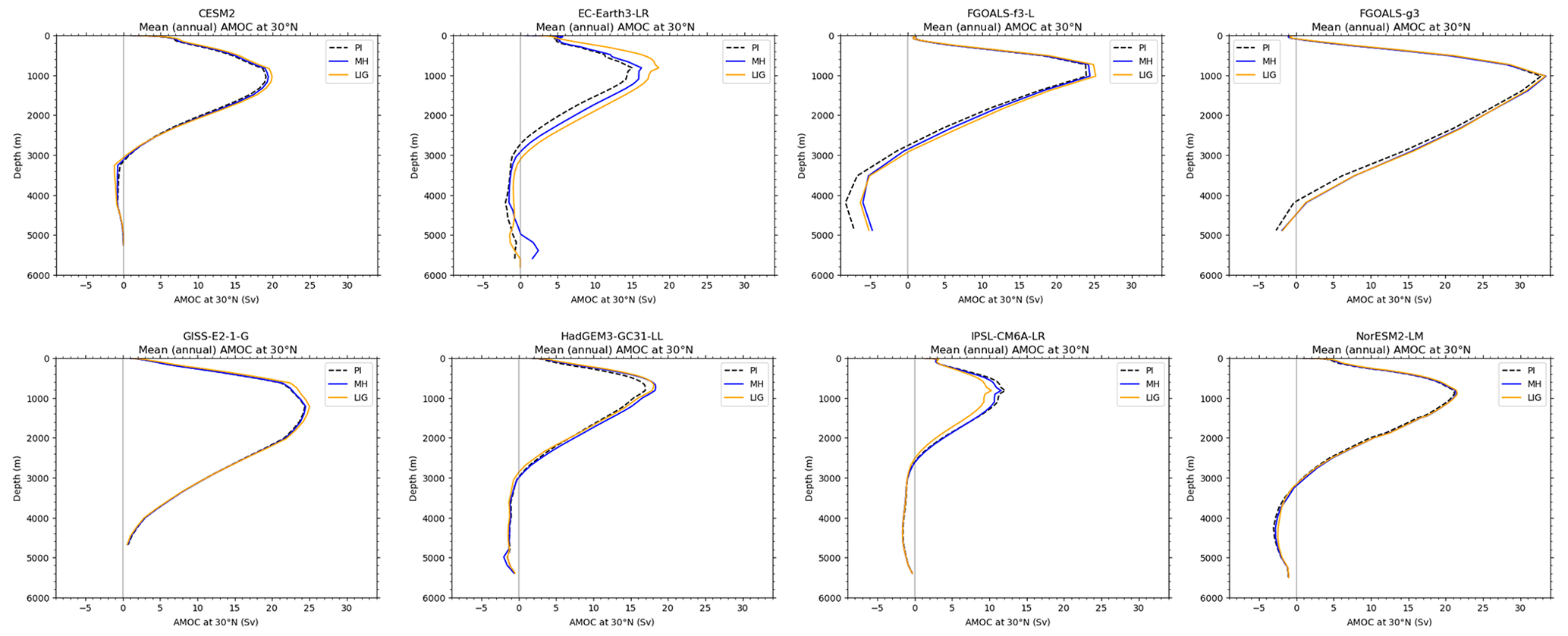
Figure 3 Mean (annual) AMOC profile at 30^∘ N in simulations. The blue line shows the AMOC profile in midHolocene, the amber line shows the AMOC profile in lig127k, and the dashed black line indicates the piControl AMOC profile.

3.2 Assessing the forced response in AMOC

Since the seasonal changes in incoming solar radiation were amplified in lig127k compared to midHolocene, it would be expected (Williams et al., 2020) that the AMOC changes seen in the lig127k experiment are a similar, but stronger version of those seen in the midHolocene experiment. This is explored by analysing the AMOC profiles at 30^∘ N for the eight models which performed both interglacial experiments (Fig. 3). Only five models (CESM2, EC-Earth3-LR, FGOALS-f3 L, HadGEM3-GC31-LL, and IPSL-CM6A-LR) show changes in AMOC in both experiments (at around 1000 m depth). The magnitude of amplification is very subtle in the CESM2 and FGOALS-f3 L models. The increases in AMOC shown between midHolocene and piControl in the HadGEM3-GC31-LR model are actually slightly larger than those seen in lig127k and attributed by Williams et al. (2020) to being a consequence of internal variability. The IPSL-CM6A-LR and EC-Earth3-LR models are the only two, out of the eight models, that demonstrate noticeable, progressive changes from piControl to midHolocene to lig127k. However, those two models show changes in opposite directions, with EC-Earth3-LR showing a positive response to the increased forcing, while the IPSL-CM6A-LR reveals a negative response.

Table 2 Tests for assessing an orbitally forced response within a model. The first two tests are based on the AMOC changes in midHolocene and lig127k compared to piControl, where changes greater than 1 Sv are in bold. The third test is based on the ratio of the AMOC changes in lig127k to the AMOC changes in midHolocene, and it is in bold when the signal ratio is greater than 1.5. The last two tests involve the internal variability. The standard deviation of the unfiltered and 25-year low-pass-filtered AMOC time series is computed by averaging the standard deviation for each model in all three experiments, weighted by the respective lengths (Table 1). The last row shows the number of experiments that have substantial low-frequency variability (r²>0.5) in each model based on the correlation between the non-filtered time series and 25-year low-pass-filtered time series. The r value of all models in all three experiments is statistically significant (p<0.05), with the exception of the FGOALS-f3 piControl experiment. It is possibly due to the short run length of just 50 years, as we use the historical experiment in this model to substitute the piControl experiment.

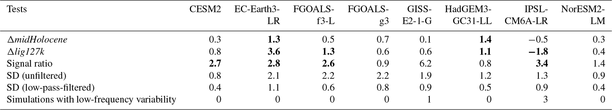
To demonstrate that AMOC responds to orbital forcing, one would look for the ensemble to simulate AMOC changes that are (i) extant, (ii) related to the strength of the forcing, (iii) detectable over the internal variability, and (iv) model-independent. Building on these criteria, we devise a series of tests that must be passed to show a forced response within a single experiment. Firstly, we test whether there is a change in AMOC, which here we arbitrarily take to be greater than 1 Sv. The changes in orbital configuration result in seasonal insolation shifts at the northern high latitudes that in lig127k are generally more than twice those in midHolocene (Otto-Bliesner et al., 2017). The AMOC response may not be linear, so the second test sets a weaker threshold and looks at whether the AMOC changes in lig127k are at least 1.5 times as large as the midHolocene ones.

Assessing whether any AMOC changes are detectable against a model's internal variability in its AMOC time series is challenging given the relative lengths of the simulations (Table 1) and the known existence of low-frequency variability in AMOC (e.g. Fischer, 2011; Shi and Lohmann, 2016; McKay et al., 2018; Bonnet et al., 2021). The relative role of internal variability is assessed by comparing its strength to the size of the changes in the long-term mean. Whether an individual model has substantial low-frequency internal variability is evaluated by firstly applying a 25-year low-pass Lanczos filter to the annual-mean AMOC time series of each simulation, and then the correlation coefficients (r) are computed between the non-filtered time series and the filtered time series in each individual simulations. If the r² value is greater than 0.5, it suggests the low-frequency variability dominates the AMOC time series (as it explains >50 % of the AMOC variations). We conclude that except for the IPSL-CM6A-LR and GISS-E2-1-G models, other models do not contain substantial low-frequency variability according to these criteria (Table 2). The IPSL-CM6A-LR is the only model for which all three experiments demonstrate substantial low-frequency variability. However, despite the CESM2 and EC-Earth3-LR models not meeting our particular criteria, the standard deviations of the filtered AMOC time series in these two models are at least half or more of the standard deviation of the non-filtered time series. Therefore, this suggests that low-frequency variability plays an important role in the CESM2 and EC-Earth3-LR models, even if it does not dominate the variability.

Only one of the eight models, EC-Earth3-LR, shows changes in AMOC that are categorised as both (i) extant and (ii) related to the strength of the forcing (Table 2). However, it is unclear if even these changes pass the third criterion of detectability above internal variability; the amplitude of the midHolocene changes is less than 1 standard deviation of the interannual time series, and there is also a confirmed presence of low-frequency variability in the EC-Earth3-LR simulation (Zhang et al., 2021).

Clearly, the results of the individual tests performed here will depend somewhat on the criteria chosen. For example, if it is the maximum AMOC across all latitudes (rather than at 30^∘ N), then both CESM2 experiments would show extant AMOC changes (Otto-Bliesner et al., 2020), but then the signal ratio is only 1.3 rather than the 2.7 in Table 2. However, two conclusions will remain robust to the many possible permutations. Overall the ensemble does not show a consistent AMOC signal from the imposed forcing changes. In fact, not a single one of the eight PMIP4 models that have performed both the midHolocene and lig127k experiments shows changes in AMOC strength that are unambiguously a response to the orbital forcing.

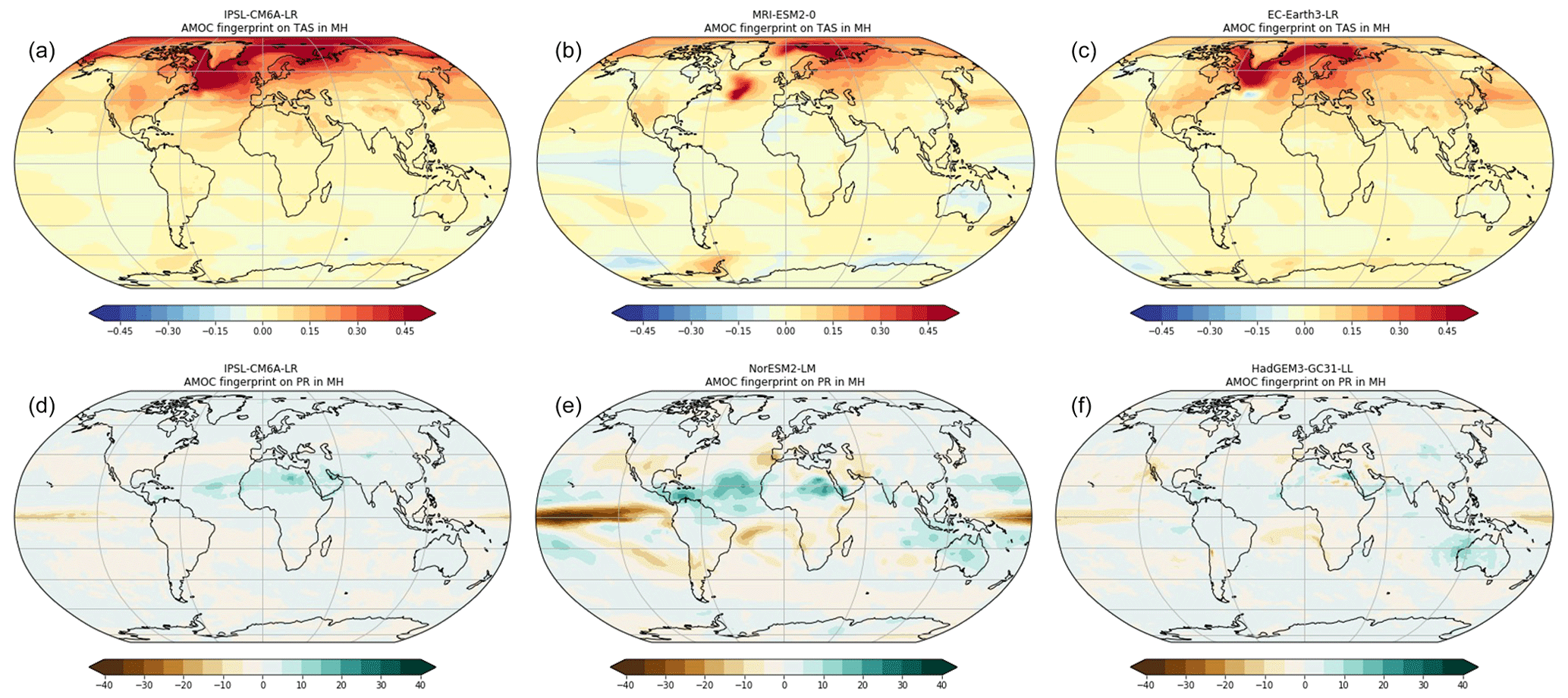
Figure 4 AMOC's fingerprint on the surface temperature (${}^{\circ }\mathrm{C}{\mathrm{Sv}}^{-\mathrm{1}}$) (a–c) and on the precipitation (% Sv⁻¹) (d–f) in midHolocene in selected PMIP4 models.

4 AMOC and global surface climate changes

We further investigate the role of AMOC in the interglacial climate system, particularly looking at the impact of AMOC on the simulated surface temperature and precipitation changes. First, we regress the temperature and precipitation at each grid box over the globe onto AMOC maximum at 30^∘ N for each simulation to obtain the local response to a 1 Sv increase (see Sect. 2). Larger regression coefficients indicate that the interdecadal variability in the AMOC has more impact on the surface temperature or precipitation changes at each grid box. There is a strong relationship between AMOC change and surface temperatures over the northern North Atlantic, and they are most obvious in the Nordic Seas, the area south of Greenland, the Labrador Sea, and along the track of the Gulf Stream (Fig. 4). This reveals that the AMOC has a noticeable influence on modulating the surface temperature through heat transport in those regions (Borchert et al., 2018; Jungclaus et al., 2014). The regression coefficients are generally higher in the Nordic Seas than that in the area south of Greenland when referring to all the 11 PMIP4 models involved (not shown). The area of influence is generally confined to the northern North Atlantic (Fig. 4), although the FGOALS-g3 L and GISS-E2-1-G models both have particularly low coefficient values (∼0.15) even there (not shown). Here we present regression coefficients from the midHolocene simulations, yet these are effectively unchanged in either the piControl or lig127k simulations (not shown).

The AMOC temperature fingerprints in the North Atlantic are accompanied by a dipole response in precipitation (Fig. 4) with roughly a 5 % decrease in the mid-latitude (30–50^∘ N) and a 5 % increase in the sub-polar and polar regions. The largest AMOC-induced precipitation changes occur in the tropics, with a reduction of about 10 %–15 % in the equatorial Pacific. FGOALS-f3 L (not shown) and NorESM2-LM show a larger decrease than other models (20 %–30 % and 30 %–40 %, respectively). The low-latitude (0–30^∘ N) North Atlantic Ocean generally reveals an increases (up to 10 %) in rainfall as the AMOC changed by 1 Sv, and it is more obvious in IPSL-CM6A-LR and NorESM2-LM. The 25 % Sv⁻¹ increase in precipitation in NorESM2-LM could be explained by the northward shifting of the Intertropical Convergence Zone (ITCZ) due to stronger AMOC in this region. NorESM2-LM shows the largest changes across the whole globe (Fig. 4) and is somewhat of an outlier. The fingerprints are very similar if computed using either piControl or lig127k simulations (not shown), demonstrating that the influence of AMOC is a robust feature in the models with minimal state dependence. It should be noted that despite these fingerprints being computed from analysis of the internal variability within individual simulations, the spatial patterns are clearly reminiscent of those seen in hosing experiments (e.g. Jackson and Wood, 2020). This demonstrates that it is valid to assume that the teleconnection patterns associated with internally generated changes in AMOC are the same as those from externally forced changes.

It is not uncommon to interpret terrestrial proxy records as being related to AMOC changes (e.g. Ayache et al., 2018) or to use compilations of proxy records to directly infer past AMOC changes (e.g. Ayache et al., 2018; Thornalley et al., 2018). Since both the AMOC fingerprints and the changes in AMOC strength have been computed, we can determine the maximum percentage of the local midHolocene climate changes that could potentially be explained by the AMOC. Such analysis could help to identify the regions to target for further proxy-based studies that contain an AMOC signal during the mid-Holocene.

Figure 5 shows the percentage of the simulated surface air temperature changes that could potentially be explained by the AMOC changes in midHolocene. The AMOC is only one of many factors influencing the local temperature changes. For example, areas with a percentage smaller than 0 can occur when the AMOC fingerprint suggests changes of the opposite sign to the actual changes. This percentage of fingerprint-estimated changes can approach, or even exceed, 100 % when the midHolocene temperature change is very small, as simulated by the model when considering all factors. Both cases indicate that the AMOC changes cannot explain the midHolocene temperature response in those areas.

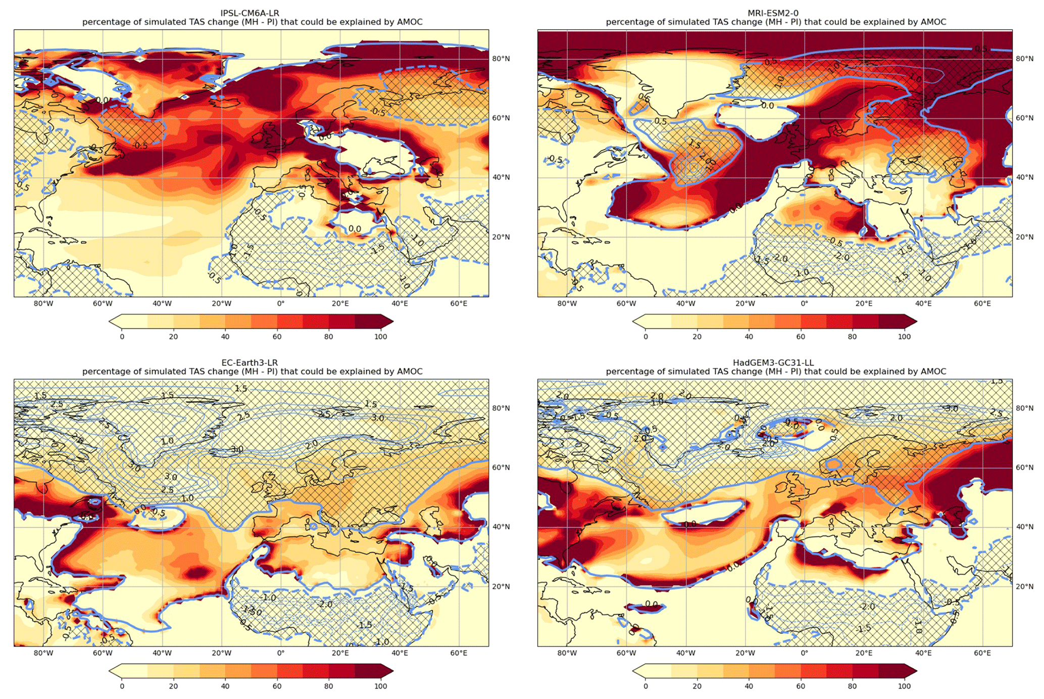
Figure 5 The maximum percentage of midHolocene-simulated surface air temperature changes that could be explained by AMOC changes (midHolocene − piControl) for four different models. These four models show a maximum AMOC strength change of 5 % or more at 30^∘ N. The overlaid contours show the magnitude of the midHolocene surface air temperature changes themselves (^∘C). Negative changes are shown with dashed lines, positive changes have solid lines, and locations where the absolute size of the changes is larger than 0.5 ^∘C are hatched.

The four models with the largest changes in maximum AMOC strength at 30^∘ N are shown in Fig. 5. In general, those places where AMOC could explain half or more of the temperature changes occur in regions where the midHolocene temperature signal itself is small. For HadGEM3-GC31-LL and EC-Earth3-LR, this means that only regions outside the northern North Atlantic are highlighted. Both IPSL-CM6A-LR and MRI-ESM2-0 show midHolocene temperature changes larger than 0.5 ^∘C in the sub-polar gyre (notable for the present-day “warming hole”; Keil et al., 2020). Despite this, those regions demonstrate some of the weakest potential impact from midHolocene AMOC changes suggested across the North Atlantic and Nordic Seas for each model (Fig. 5). AMOC-related changes cannot explain any of the temperature changes seen in the other models (not shown), as they see very small changes in the AMOC itself (Table 1).

After analysing all the models, we conclude that the AMOC does not play a globally important role in explaining the temperature changes, and the role may be secondary to other factors even in the North Atlantic. This conclusion also applies to sea surface temperature and holds for lig127k as well (not shown). A similar analysis has also been performed to look at the AMOC-related precipitation changes (see Supplement). The vast majority of the globe has an estimated contribution of 10 % or less of the midHolocene and lig127k precipitation changes, questioning whether reconstructed precipitation changes can be used as inferring information about the AMOC.

5 Discussion

Past changes in overall AMOC strength, especially its depth integral, are difficult to reconstruct. Many previous studies have instead focused on examining individual components of the AMOC or inferred changes in deep water mass geometry (e.g. Kissel et al., 2013; Solignac et al., 2004). However, one proxy technique is to use sedimentary $\mathrm{Pa}/\mathrm{Th}$ (e.g. Yu et al., 1996; McManus et al., 2004), although modern geochemical observations highlight the contribution of other factors controlling the Pa and Th distribution (Hayes et al., 2013). For example, Missiaen et al. (2020) using a $\mathrm{Pa}/\mathrm{Th}$-enabled model revealed that the changes in biogenic particle fluxes can affect the Atlantic $\mathrm{Pa}/\mathrm{Th}$ records, and the particle flux changes have been suggested to cause far-field $\mathrm{Pa}/\mathrm{Th}$ variations as well.

High-resolution Holocene $\mathrm{Pa}/\mathrm{Th}$ reconstructions from the North Atlantic (Hoffmann et al., 2018; Lippold et al., 2019) show no observable changes, unlike the faint AMOC weakening in the Holocene shown by low-resolution $\mathrm{Pa}/\mathrm{Th}$ data (Negre et al., 2010; Lippold et al., 2016; McManus et al., 2004; Gherardi et al., 2009; Ng et al., 2018). As the high-resolution $\mathrm{Pa}/\mathrm{Th}$ records are both single-site studies from the sub-tropical north-western Atlantic, it is unclear how well they represent the overall AMOC strength (Hoffmann et al., 2018; Lippold et al., 2019). Taken together, the $\mathrm{Pa}/\mathrm{Th}$ records indicate relatively similar AMOC strength for the mid-Holocene and preindustrial. There are fewer sedimentary $\mathrm{Pa}/\mathrm{Th}$ records for the Last Interglacial, although they also do not indicate substantial changes in AMOC strength (Guihou et al., 2010, 2011; Böhm et al., 2015; Jonkers et al., 2015)

Reconstruction of changes in the density profile of the Florida Straits shows little change in the strength of the upper limb of the AMOC over the past 8000 years (Lynch-Stieglitz et al., 2009). Just under half the Florida Strait flow is associated with the AMOC, with the remainder relating to the wind-driven surface gyre circulation. Therefore the reported slight increase (4 Sv increase on a flow of 28–32 Sv) over the past 8000 years may be attributed instead to a strengthening of the wind-driven gyre circulation in the western Atlantic (Lynch-Stieglitz et al., 2009). To our knowledge, an equivalent reconstruction does not exist for the Last Interglacial. However, a recent benthic δ¹³C compilation shows no obvious changes in the spatial structure (latitudinal and depth extent) of the North Atlantic Deep Water (NADW) between the Last Interglacial and mid-Holocene, and suggests that the mean NADW transport was similar (Bengtson et al., 2021).

In summary, no palaeo-reconstructions demonstrate substantive changes in the depth-integrated AMOC strength between either of the two interglacial states and piControl. This, therefore, does not disagree with the PMIP4 ensemble demonstrating no consistent response in overall AMOC strength to the changes in orbital forcing (Sect. 3.2). However, it is not yet possible to confidently assert that the PMIP4 ensemble is simulating the correct response. Two obstacles need to be overcome before that can happen: (i) a greater number of proxy records obtained throughout the basin, especially during the Last Interglacial, and (ii) a significant reduction in uncertainties in the proxy data and their interpretation. Greater application of proxy system models (e.g. Burke et al., 2011) and proxy-enabled ocean general circulation models (e.g. Sasaki et al., 2022; van Hulten et al., 2018), possibly combined with data assimilation approaches (e.g. Rempfer et al., 2017; Osman et al., 2021), could potentially resolve the latter.

Further research into the various flow components of AMOC and their respective coupling to the climate system is required before one could conclude that there were no significant interglacial changes in AMOC. It is also worth noting that all the simulations and analysis here are looking at equilibrated time slice simulations, rather than transient simulations (e.g. Bader et al., 2020; Braconnot et al., 2019). Our conclusion of a minimal role for overall AMOC strength changes does not, therefore, apply to abrupt events where an AMOC response has long been identified (LeGrande and Schmidt, 2008).

6 Conclusions

The AMOC during interglacial conditions has been investigated in this study using the 12 PMIP4 models that performed the midHolocene and lig127k experiments, and the changes have been compared to the AMOC simulated for the piControl experiment. Obvious differences in the AMOC strength between individual models reveal that the climate models are still struggling to accurately simulate the strength of the AMOC, as well as to capture the depth profile of the AMOC (Eyring et al., 2021). The overall AMOC strength between either lig127k or midHolocene and piControl has not markedly changed in individual simulations (Fig. 1), nor has its spatial meridional structure changed in the ensemble mean (Fig. 2). The two models that show the largest changes in the lig127k experiment change in the opposite direction. Many of the models show changes in amplitude that could be explained by internal variability, rather than a forced response (Williams et al., 2020). It therefore seems the changes in orbital forcing in both the lig127k and midHolocene experiments have very limited impact on the overall AMOC strength. This finding is not inconsistent with available proxy reconstructions.

The surface climate fingerprints arising from internal variability in the AMOC remain largely unchanged between midHolocene, lig127k, and piControl, although there are variations amongst the models in those patterns (Fig. 4). We demonstrate that, unsurprisingly, the AMOC does not play a globally important role in explaining temperature changes in the midHolocene or lig127k experiments (Fig. 5). Combined with the inconsistent simulated forced response of AMOC during the PMIP4 time slice simulations, the fingerprint analysis suggests that the overall AMOC strength changes should only be invoked to explain climate changes during abrupt events in interglacials.

Appendix A: ESGF digital object identifier (DOI)

Otto-Bliesner et al. (2020)Zhang et al. (2021)Zheng et al. (2020)Zheng et al. (2020)Kelley et al. (2020)Williams et al. (2020)Lurton et al. (2020)Seland et al. (2020)Volodin et al. (2018)Scussolini et al. (2019)Yukimoto et al. (2019)Yeung et al. (2021)

Table A1 Digital object identifier (DOI) for each simulation from CMIP6. The web address can be created manually by adding https://dx.doi.org/10.22033/ESGF/ in front of each DOI. NA in the table stands for not available and indicates either that the simulation has not been performed or that streamfunction data have not been uploaded to the Earth System Grid Federation.