Evaluating seasonal sea-ice cover over the Southern Ocean at the Last Glacial Maximum

Southern hemispheric sea-ice impacts ocean circulation and the carbon exchange between the atmosphere and the ocean. Sea-ice is therefore one of the key processes in past and future climate change and variability. As climate models are the only tool available to project future climate change, it is important to assess their performance against observations for a range of different climate states. The Last Glacial Maximum (LGM, ∼21 000 years ago) represents an interesting target as it is a relatively well-documented period with climatic conditions very different from preindustrial conditions. Here, we analyze the LGM seasonal Southern Ocean sea-ice cover as simulated in numerical simulations as part of the Paleoclimate Modelling Intercomparison Project (PMIP) phases 3 and 4. We compare the model outputs to a recently updated compilation of LGM seasonal Southern Ocean sea-ice cover and summer sea surface temperature (SST) to assess the most likely LGM Southern Ocean state. Simulations and paleo-proxy records suggest a fairly well-constrained glacial winter sea-ice edge between 50.5 and 51^∘ S. However, the spread in simulated glacial summer sea-ice is wide, ranging from almost ice-free conditions to a sea-ice edge reaching 53^∘ S. Combining model outputs and proxy data, we estimate a likely LGM summer sea-ice edge between 61 and 62^∘ S and a mean summer sea-ice extent of 14–15×10⁶ km², which is ∼20 %–30 % larger than previous estimates. These estimates point to a higher seasonality of southern hemispheric sea-ice during the LGM than today. We also analyze the main processes defining the summer sea-ice edge within each of the models. We find that summer sea-ice cover is mainly defined by thermodynamic effects in some models, while the sea-ice edge is defined by the position of Southern Ocean upwelling in others. For models included in both PMIP3 and PMIP4, this thermodynamic or dynamic control on sea-ice is consistent across both experiments. Finally, we find that the impact of changes in large-scale ocean circulation on summer sea-ice within a single model is smaller than the natural range of summer sea-ice cover across the models considered here. This indicates that care must be taken when using a single model to reconstruct past climate regimes.

1 Introduction

Antarctic sea-ice plays an important role in the earth’s climate system, affecting marine productivity, air-sea gas exchange, air-sea heat fluxes, surface water density, and surface albedo. It can both impact and respond to changes in bottom-water formation and Southern Ocean (SO) circulation, and therewith impact large-scale heat transport and ocean carbon uptake. While Arctic sea-ice cover has significantly decreased over the last few decades, Antarctic sea-ice cover has been more dynamic. It slowly expanded from the late 1970s until 2016, and then sharply declined for the next 3 years (Eayrs et al., 2021). Doddridge and Marshall (2017) have shown that on a seasonal timescale, SO sea-ice was responding to changes in the southern annual mode (SAM), with a positive phase of the SAM leading to lower SO sea surface temperatures (SST) and a larger sea-ice extent. However, on longer timescales, a positive phase of the SAM can lead to a SO warming due to the enhanced upwelling of relatively warm circumpolar deep waters (Ferreira et al., 2015). Due to continued anthropogenic emissions of carbon dioxide, the southern hemispheric westerly winds are projected to strengthen and to shift towards positive phases of the SAM (Zheng et al., 2013), impacting SO circulation and sea-ice cover further (Mayewski et al., 2017). Given that the SO has accounted for ∼40 % of the oceanic anthropogenic CO₂ uptake between 1870 and 1995 (Landschützer et al., 2015; Sabine et al., 2004; Frölicher et al., 2015; Mikaloff-Fletcher et al., 2006; Watson et al., 2020), it is crucial to better understand the processes that impact Antarctic sea-ice cover. Specifically, seasonal changes in sea-ice can significantly affect SO dynamics through buoyancy (Marzocchi and Jansen, 2017) and lead to changes in the atmosphere-ocean carbon exchange (Haumann et al., 2016). Understanding changes in sea-ice and their natural drivers at different timescales and under different boundary conditions will allow us to better project future sea-ice changes.

The Last Glacial Maximum (LGM, ∼21 000 years ago) featured large continental ice-sheets over North America and Eurasia (e.g., Carlson and Winsor, 2012; Clark et al., 2009), as well as an extended Antarctic ice-sheet (Bentley et al., 2014), and an atmospheric CO₂ concentration of ∼185 ppm (Marcott et al., 2014). Despite significant progress in characterizing the LGM sea-surface conditions (e.g., Waelbroeck et al., 2009), oceanic circulation (e.g., Howe et al., 2016; Lynch-Stieglitz et al., 2007; Meissner et al., 2003; Menviel et al., 2017; Skinner et al., 2017), and mechanisms leading to a lower atmospheric CO₂ concentration (e.g., Kohfeld and Chase, 2017), significant uncertainties remain. Some of these uncertainties lie in characterizing seasonal Antarctic sea-ice. While LGM Antarctic sea-ice was first reconstructed in 1981 (CLIMAP-Project-Members, 1981), the proxy compilation of Gersonde et al. (2005) is nowadays routinely used to provide estimates of LGM sea-ice cover. Since 2005, additional SO sea-ice data have been published (Allen et al., 2011; Benz et al., 2016; Ferry et al., 2015; Ghadi et al., 2020; Nair et al., 2019; Xiao et al., 2016), and recently merged into an updated compilation (Lhardy et al., 2021). Within this updated sea-ice compilation, certain cores also contain summer SST estimates. We use this sea-ice proxy data along with the summer SST proxy data to better constrain the minimum and maximum LGM sea-ice cover.

Although paleo-proxy records are an invaluable tool to reconstruct the climate system, they are sometimes scarce or completely absent over entire regions. Climate models can help fill these gaps, as they provide a full 3-dimensional and dynamically consistent representation of the climate system. However, as climate models are not perfect representations of reality, it is important that we continually evaluate their performance. The Paleoclimate Intercomparison Project (PMIP) has been set up to evaluate and compare model performances across consistent boundary conditions (Kageyama et al., 2017). Results from the PMIP phase 4 are currently being released (Kageyama et al., 2021), while phases 1–3 are available to the public (https://pmip3.lsce.ipsl.fr, last access: 15 March 2022).

The PMIP2 LGM simulations suggested that simulated LGM Antarctic sea-ice cover did not reflect the zonal variability nor the seasonality seen in proxy reconstructions (Roche et al., 2012). The PMIP3 LGM simulations have also been analyzed, however not regionally, with results highlighting large intermodel differences in annual mean, minimum and maximum Antarctic sea-ice areas, and suggesting most PMIP3 models underestimate austral winter sea-ice cover in comparison to proxy data (Sime et al., 2016; Marzocchi and Jansen, 2017). Therefore, a regional analysis of seasonal LGM sea-ice simulated by PMIP3 models is lacking. Furthermore, no seasonal sea-ice analysis of PMIP4 simulations under LGM boundary conditions has yet been performed.

Here, we assess the minimum and maximum SO sea-ice extent as simulated in LGM PMIP3 and PMIP4 experiments. To better assess intramodel versus intermodel variability, a suite of LGM sensitivity experiments performed with the LOVECLIM model of intermediate complexity are also included. The PMIP3, PMIP4 and LOVECLIM experiments are compared to available sea-ice and SST paleo-proxy data, allowing us to determine the best model data fit. Combining models and proxy data, we can provide an updated estimate of seasonal SO sea-ice cover during the LGM. Furthermore, we analyze the processes that lead to the intermodel differences in summer sea-ice extent at the LGM.

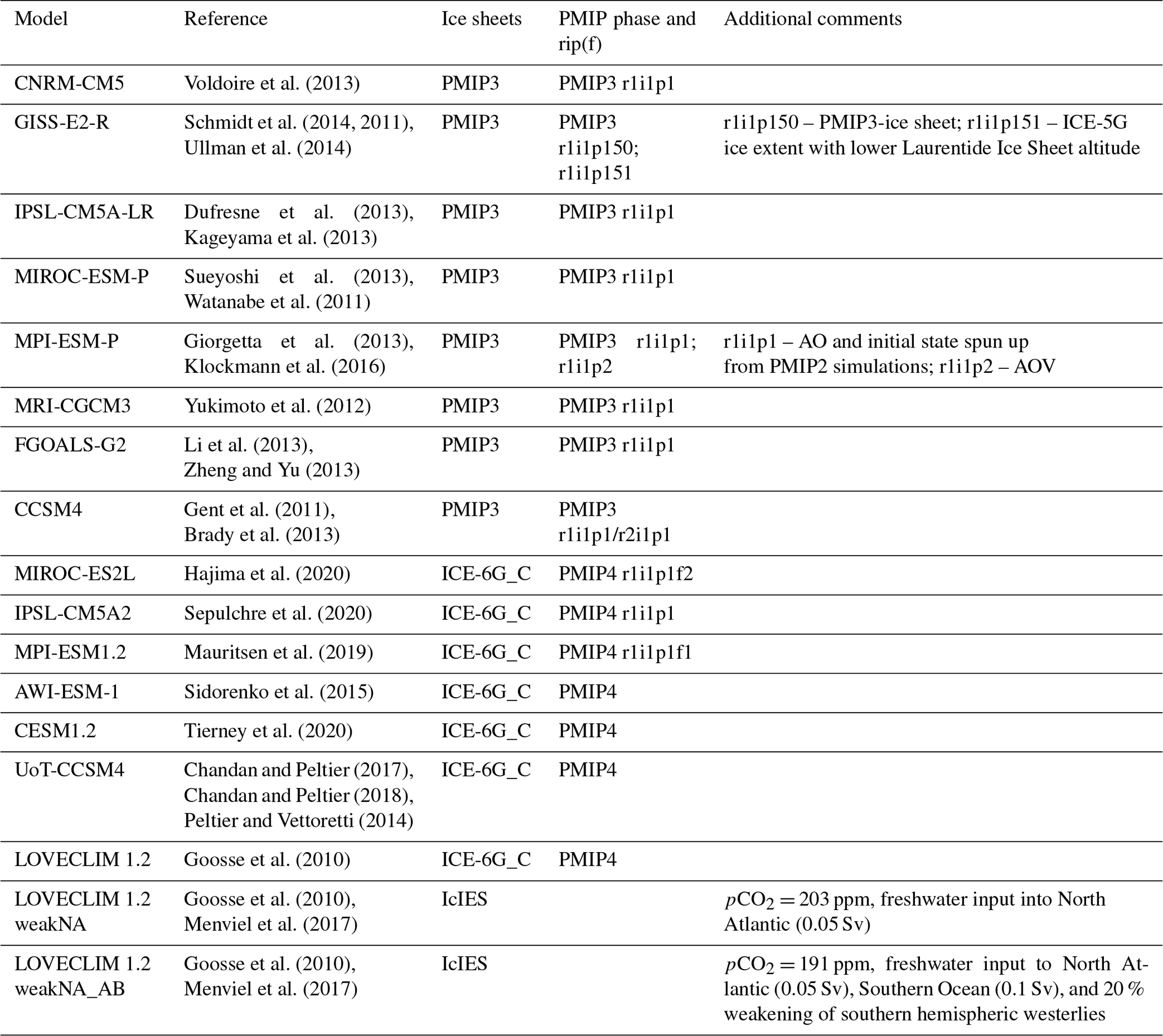
Voldoire et al. (2013)Schmidt et al. (2014, 2011)Ullman et al. (2014)Dufresne et al. (2013)Kageyama et al. (2013)Sueyoshi et al. (2013)Watanabe et al. (2011)Giorgetta et al. (2013)Klockmann et al. (2016)Yukimoto et al. (2012)Li et al. (2013)Zheng and Yu (2013)Gent et al. (2011)Brady et al. (2013)Hajima et al. (2020)Sepulchre et al. (2020)Mauritsen et al. (2019)Sidorenko et al. (2015)Tierney et al. (2020)Chandan and Peltier (2017)Chandan and Peltier (2018)Peltier and Vettoretti (2014)Goosse et al. (2010)Goosse et al. (2010)Menviel et al. (2017)Goosse et al. (2010)Menviel et al. (2017)

Table 1 Models analyzed in this study, the PMIP phase they pertain to, and the ice-sheet forcing that was used. When applicable, the ensemble member is specified using rip(f) nomenclature (https://pcmdi.llnl.gov/CMIP6/Guide/dataUsers.htm last access: April 4th, 2022). The Ice sheet model for Integrated Earth system Studies (IcIES) forced by climatic outputs from the Model for Interdisciplinary Research on Climate (MIROC) (Abe-Ouchi et al., 2013). The atmospheric CO₂ concentration (pCO₂) for PMIP3 and PMIP4 experiments is 185 and 190 ppm, respectively. pCO₂ for the two LOVECLIM sensitivity experiments is given.

2 Methods

2.1 LGM numerical simulations

In this study, we include all PMIP3 and PMIP4 LGM simulations which provide sea-ice variables in the PMIP3 and PMIP4 database (Table 1). Each LGM simulation follows either the PMIP3 or PMIP4 protocol (Braconnot and Kageyama, 2015; Kageyama et al., 2017). The PMIP3 protocol calls for all models to use the same ice sheet reconstruction, while the PMIP4 protocol allows the use of either the original PMIP3 ice sheet to facilitate comparison with earlier simulations, or one of the newer reconstructions ICE-6G_C (Argus et al., 2014; Peltier et al., 2015) and GLAC-1D (Ivanovic et al., 2016). In total, data from eight models were obtained for PMIP3 and from six models for PMIP4 (Table 1). Three PMIP3 models (CCSM4, GISS-E2-R, MPI-ESM-P) submitted two different simulations. These simulations differed because of a difference in the initial state (CCSM4), or small changes in the physics of the model (GISS-E2-R and MPI-ESM-P). Following Sime et al. (2016), we chose to average the simulations for the models that submitted two LGM runs, yielding one output per model.

We also include three additional LGM simulations performed with the earth system model of intermediate complexity, LOVECLIM (Goosse et al., 2010). LOVECLIM consists of an ocean general circulation model, a dynamic-thermodynamic sea-ice model, coupled to a quasi-geostrophic atmospheric model, a dynamic vegetation model and a carbon cycle model (Goosse et al., 2010). One of the LOVECLIM simulations follows the PMIP4 protocol, while two additional simulations were obtained by transiently forcing the model between 35 000 and 20 000 years before the present with appropriate boundary conditions (i.e., orbital parameters, northern hemispheric ice-sheet topography and albedo) (Menviel et al., 2017). During the 35 ka spin-up the atmospheric CO₂ concentration was set at 190 ppm, after which CO₂ was a prognostic variable. In these simulations the oceanic circulation was altered by (i) adding 0.05 Sv of freshwater to the North Atlantic to simulate a weaker and shallower North Atlantic Deep Water (NADW) formation at the LGM compared to preindustrial times (simulation V3LNAw in Menviel et al., 2017, here referred to as weakNA), (ii) by adding 0.05 Sv of freshwater to the North Atlantic, 0.1 Sv to the SO, as well as by weakening the southern hemispheric westerlies by 20 % to simulate a weaker LGM NADW and Antarctic Bottom Water (AABW) formation (simulation V3LNAwSOwSHWw in Menviel et al., 2017, here referred to as weakNA_AB). Atmospheric CO₂ was calculated prognostically in these experiments and was 203 ppm in weakNA and 191 ppm in weakNA_AB, compared to 185 ppm in the PMIP3 protocol, and 190 ppm in the PMIP4 protocol. These two simulations will be referred to as the “LOVECLIM sensitivity runs”. They were chosen because they provided the best model-data fit against a range of paleo-proxy records, including phosphate, δ¹³C, radiocarbon ventilation ages, and neodymium isotopic signature (Menviel et al., 2017, 2020), thus indicating an appropriate oceanic circulation representation. The three LOVECLIM simulations can provide information on the impact of oceanic circulation differences on SO sea-ice and SST, and thus allow us to assess intramodel versus intermodel differences.

To facilitate the comparison, we used bilinear interpolation to standardize each model to a $\mathrm{1}{}^{\circ }\times \mathrm{1}{}^{\circ }$ grid with the CDO software (Climate Data Operators, Schulzweida et al., 2014).

2.2 Proxy data

The numerical simulations are compared to a compilation of 149 proxy records covering the LGM (see Table S1 in the Supplement, Allen et al., 2011; Benz et al., 2016; Ferry et al., 2015; Gersonde et al., 2005; Ghadi et al., 2020; Nair et al., 2019; Xiao et al., 2016). Quantitative SST was reconstructed at 138 locations, proxies for winter sea-ice presence or concentration were available at 149 locations and proxies for summer sea-ice presence were available at 132 locations. The SSTs were derived from diatom-based transfer functions (Crosta et al., 1998; Esper and Gersonde, 2014a) while winter and summer sea-ice extents were derived either from the relative abundance of sea-ice indicator diatoms, or the Fragilariopsis curta group and F. obliquecostata (Gersonde et al., 2005), or diatom-based transfer functions whenever possible (Crosta et al., 1998; Esper et al., 2014b). Relative abundances of the indicator diatoms above 3 % are thought to indicate the presence of sea-ice over the core site (mean sea-ice extent north of the core site) while relative abundances between 1 % and 3 % suggest the episodic presence of sea-ice over the core site (mean sea-ice edge south of the core site but maximum sea-ice edge north of the core site). In this study, we characterize the relative abundance of >3 % as evidence of sea-ice and the relative abundance between 1 % and 3 % as evidence for possible sea-ice. Quantitative values were considered to indicate the presence of winter sea-ice when they were above the root mean square error of prediction (RMSEP) on the validation models, generally around 10 % for winter sea-ice (Crosta et al., 1998; Esper et al., 2014b). Quantitative values were always below the RMSEP of ∼10 % for summer sea-ice in the validation model.

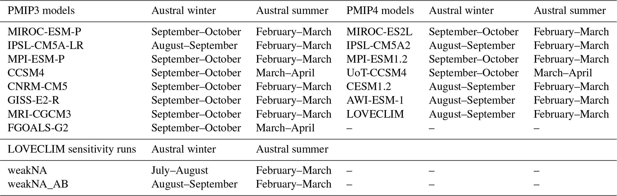
Table 2 Austral winter and austral summer months used for each simulation.

2.3 Definitions of sea-ice edge, extent, seasonality, and regions

We analyze the climatology of Antarctic sea-ice extent and define the 2 months of maximum and minimum sea-ice for each individual model (Table 2). These 2 months of maximum and minimum sea-ice are used consistently throughout the study and will hereafter be referred to as each model’s austral “winter” and “summer”, respectively. We note that using a 2-month average leads to a larger summer and a smaller winter sea-ice extent, compared to what would be obtained from a 1-month average. However, we believe that a 2-month average is more appropriate for a comparison with proxy records. We also analyze simulated sea-ice within specific regions which we refer to by the ocean basin the region lies in: Atlantic, Pacific, and Indian Sector.

The sea-ice edge is defined as the 15 % sea-ice concentration isoline. We calculate this by zonally averaging across all longitudes for each latitude band, then determining at which latitude the model simulates a minimum of 15 % sea-ice concentration. For model simulations that do not reach 15 % of sea-ice concentration in some regions of the SO, we average only over the remaining regions with sufficient sea-ice cover. For model simulations that do not reach 15 % sea-ice concentration in any region, we define the latitude of their sea-ice edge as the latitude of the Antarctic coast. It is important to note that although a model’s sea-ice edge gives insights into its sea-ice characteristics, it is not always an accurate representation of how much total sea-ice a model simulates. Due to this, we also calculate the total sea-ice extent for each model (using a cut-off limit of 15 % in concentration).

To calculate the multi-model mean (MMM), we average sea-ice concentration over each grid cell for all models (PMIP3, PMIP4, and LOVECLIM sensitivity runs separately). We then calculate the 15 % sea-ice concentration isoline of each MMM. To calculate the standard deviation, we similarly compute a standard deviation value for each individual grid cell, before adding and subtracting that standard deviation (σ) of sea-ice concentration from the MMM for each grid cell. The ±1σ then represents the 15 % sea-ice concentration isoline calculated from the MMM ±1σ. Notably, this creates a non-symmetric standard deviation isoline as each grid cell has its own MMM (and σ) value, calculated independently from any surrounding grid cells.

3 Results

Figure 1 shows the austral winter and austral summer mean LGM sea-ice extent as simulated by each model considered here as well as the MMM and ±1σ for the PMIP3, PMIP4 and LOVECLIM models. For comparison, available paleo-proxy records are overlaid for austral winter and austral summer. The simulated annual mean LGM sea-ice extent is shown for all the models in Fig. S1.

Figure 1 Simulated summer and winter sea-ice edge compared to proxy data for PMIP3 (a–d) and PMIP4 (e–h) models as well as LOVECLIM sensitivity runs (i–l). The left panels for each group show simulated austral summer sea-ice concentration at 15 % (a, c, e, g, i, k) and the right panels show simulated austral winter sea-ice concentration at 15 % (b, d, f, h, j, l). The top panels for each group show individual model results (a, b, e, f, i, j) while the bottom panels show the multi-model mean ±1σ (c, d, g, h, k, l). Blue, black, and red points represent the sediment core proxy data used for the study.

3.1 Simulated austral winter SO sea-ice extent and comparison with winter sea-ice proxy records

During austral winter, the simulated zonally averaged MMM sea-ice edge for PMIP3 models lies at ∼51.5^∘ S with 1σ equating to 1.5^∘ north and 5^∘ south of the MMM (Fig. 1d, Table 3). Regional differences are found across the models. In the Indian Ocean sector (20–147^∘ E), the standard deviation increases to the south due to GISS-E2-R (cyan) simulating a sea-ice edge reaching 59.5^∘ S in that sector, compared to the Indian sector MMM of 50.5^∘ S. South of the MMM, the standard deviation is also large in the Pacific sector (147^∘ E to 68^∘ W) as CNRM-CM5 (black) simulates a sea-ice edge at ∼59.5^∘ S compared to the Pacific sector MMM of ∼56.5^∘ S. There is higher model agreement in the Atlantic sector (68^∘ W to 20^∘ E) leading to one standard deviation of only $+\mathrm{0.5}/-\mathrm{1.5}$^∘ in that region.

Similar to PMIP3 models, PMIP4 models simulate a MMM sea-ice edge at ∼51^∘ S during austral winter with a zonally averaged standard deviation of 2^∘ north and 5^∘ south of the MMM (Fig. 1h, Table 2). The UoT-CCSM4 (orange) simulates the largest sea-ice cover with a sea-ice edge at ∼48^∘ S. Conversely, MIROC-ES2L (purple) simulates significantly less sea-ice than all other models, despite having a slightly extended sea-ice edge north of 60^∘ S in the Atlantic sector. IPSL-CM5A2 (green) also simulates limited sea-ice cover in the Pacific sector. Due to MIROC-ES2L's extended sea-ice edge in the Atlantic and a relatively good agreement between the other six models in that region, standard deviation is smallest in the Atlantic sector with values of $+\mathrm{1}{}^{\circ }/-\mathrm{3}{}^{\circ }$.

During austral winter both LOVECLIM sensitivity runs simulate similar sea-ice cover despite the different circulation forcing. The MMM sea-ice edge is simulated at ∼51.5^∘ S with a standard deviation of 0.5^∘ north and 1^∘ south. The PMIP3, PMIP4 and LOVECLIM models thus simulate similar MMM sea-ice edge locations between 51 and 51.5^∘ S. There are slight regional differences due to a few models displaying a different sea-ice edge in a particular sector, however, the zonally averaged standard deviations produce similar values for PMIP3 and PMIP4. With only two similar models included in the LOVECLIM sensitivity MMM, the standard deviation is much smaller.

We next compare the simulations with proxy data of sea-ice presence or absence. A relative abundance of F. obliquecostata greater than 3 % (Fig. 1 blue points) indicates the presence of sea-ice, relative abundances of F. obliquecostata between 1 % and 3 % suggest the possible presence of sea-ice (Fig. 1 black points), and core locations with a relative abundance of F. obliquecostata <1 % indicate ice-free conditions (Fig. 1 red points). We use these data points to calculate a model data sea-ice agreement percentage, based on whether the model simulation correctly or incorrectly simulates the sea-ice state at the location of the proxy data. For these calculations, we characterize the possible presence of sea-ice (1 %–3 % [F. obliquecostata]) as ice-free.

All three MMMs for austral winter display a model data sea-ice agreement between 83 % and 84 % (Fig. 1, Table 3). Of the proxy data points 4 indicate the presence of sea-ice extending past 50^∘ S, all located within the Atlantic sector and into the westernmost edge of the Indian sector. Both the PMIP3 and PMIP4 MMMs simulate this feature as their sea-ice edge extends equatorward of 50^∘ S within the Atlantic sector. With respect to individual model performance, FGOALS-G2 (pink) simulates the highest model data sea-ice agreement with 87 %, corresponding to a simulated sea-ice edge of 50.5^∘ S. With an extended sea-ice edge in the Atlantic and slightly retreated sea-ice edge within the Pacific, FGOALS-G2 seems to most accurately simulate the regional distribution of the proxy data. The data and modeling constraints thus suggest that the LGM austral winter sea-ice (WSI) edge was likely between 50.5 and 51^∘ S and the mean LGM austral WSI extent was likely around 35–36×10⁶ km².

3.2 Simulated austral summer SO sea-ice extent and comparison with summer sea-ice proxy records

A larger spread among the models is obtained during austral summer (Fig. 1a, c), with a MMM sea-ice edge at ∼62.5^∘ S and a zonally averaged standard deviation of 5^∘ north and 11^∘ south of the PMIP3 MMM. The largest sea-ice cover is simulated by CCSM4 (orange) with a sea-ice edge at ∼55.5^∘ S. Three models (CNRM-CM5, black; GISS-E2-R, cyan; IPSL-CM5A-LR, green) only simulate sea-ice around the Ross and Weddell Seas and are otherwise ice-free. CNRM-CM5 (black) simulates the least amount of sea-ice at or above 15 % concentration with sea-ice only simulated in a small region of the Ross Sea (Fig. 1a).

The austral summer MMM in PMIP4 models is larger than for PMIP3 with a sea-ice edge at ∼59.5^∘ S and a zonally averaged standard deviation of 4.5^∘ north and 10.5^∘ south of the MMM (Fig. 1g, Table 2). Similar to austral winter, UoT-CCSM4 (orange) simulates the largest sea-ice cover with a sea-ice edge reaching ∼53^∘ S while MIROC-ES2L (purple) and IPSL-CM5A (green) simulate the least amount of sea-ice with sea-ice only found over the Ross and Weddell Seas.

There are slightly larger sea-ice differences between the two LOVECLIM sensitivity runs during austral summer than winter. The MMM sea-ice edge is simulated at ∼59^∘ S with a standard deviation of 0.5^∘ north and 1^∘ south of the MMM. WeakNA (dotted yellow) has more regional variability than weakNA_AB (dash-dot yellow). Due to the small standard deviation simulated by LOVECLIM, the ±1σ contour lines are hard to distinguish from the MMM for both austral winter and austral summer. For all three groups, the simulated MMM summer sea-ice (SSI) edge ranges from 59 to 62.5^∘ S with one standard deviation ranging from 5^∘ north and 11^∘ south of their MMMs. Thus, the SSI edge is more poorly constrained than the WSI edge.

The simulated summer sea-ice extent can also be compared to paleo-proxy records. Only 6 core locations out of 132 indicate the presence of SSI while 7 additional cores from the Atlantic sector of the SO suggest the possible presence of SSI. The remaining 119 core locations indicate ice-free conditions (including 64 cores with 0 % relative abundance of F. obliquecostata). Of the six locations indicating the presence of sea-ice, three cores are located in the Indian sector at ∼63^∘ S south of the MMM for all three model groups, whereas the other three are located in the Atlantic sector at ∼53^∘ S, north of the MMM for all three model groups (Fig. 1). However, two of the three cores within the Atlantic sector indicating LGM SSI fall inside the PMIP4 +1σ contour line (Fig. 1g). Five of the seven locations indicating the possible presence of SSI are located north of all three MMMs, but again on or inside the PMIP4 +1σ contour line (Fig. 1g). We note that the eight locations from the Atlantic sector representing a presence or possible presence of SSI are bordered by cores suggesting ice-free conditions, possibly indicating a sea-ice tongue protruding from the Weddell Sea. The reader should bear in mind that with limited proxy data points indicating SSI and multiple models simulating limited SSI, it is not uncommon to record the same summer model data sea-ice agreement percentage across different model simulations.

With only six proxy data points indicating SSI, the PMIP3 MMM, which displays the smallest SSI extent across MMMs, shows the highest model data sea-ice agreement (Table 3). In terms of individual models, it is clear some models simulate too much sea-ice (CCSM4 and UoT-CCSM4, orange), while other models simulate too little (CNRM-CM5, black; GISS-E2-R, cyan; MIROC-ESM-P and MIROC-ES2L, purple; IPSL-CM5A-LR and IPSL-CM5A2, green). With only six proxy core locations indicating SSI, it is not possible to extrapolate an estimate of the LGM sea-ice edge strictly based on these data. However, we note that the highest individual model agreement is achieved by MRI-CGCM3 (blue), with an agreement of 98 % and a sea-ice edge at 62.5^∘ S, which also corresponds to the PMIP3 MMM. On the other hand, the data-model agreement significantly drops for models simulating a large sea-ice cover. CCSM4 (orange) and UoT-CCSM4 (orange), with sea-ice edges of 55.5 and 53^∘ S respectively, simulate sea-ice in locations where the proxy records suggest ice-free conditions in all sectors of the SO. They are thus most likely overestimating austral SSI cover.

3.3 Simulated LGM summer SO SST and comparison with proxy records

To better constrain the extent of LGM SSI , we look into the proxy estimates of LGM summer SST data. We first assess the relationship between zonally averaged simulated austral summer SSTs in the SO (between 50 and 75^∘ S) and the simulated sea-ice edge and extent (Fig. 2a, b). The relationship between simulated summer SO SST and SSI edge or extent can be approximated by a linear fit, with R² values of 0.90 and 0.81, respectively (Fig. 2a, b). Similarly, this relationship is also seen during austral winter with R² values of 0.80 and 0.88, respectively (Fig. 5).

The mean LGM summer SO SST can be estimated from proxy records to be 1.52 ± 0.67 ^∘C. Using the mean SST reconstructed from the proxy records and the linear relationship estimated based on the simulations, we calculate a proxy SSI extent estimate of 15.90 × 10${}^{\mathrm{6}}\pm \mathrm{3.25}\times {\mathrm{10}}^{\mathrm{6}}$ km² and a mean sea-ice edge estimate of 61^∘ S ± 2.25^∘. The models closest to these proxy sea-ice estimates are weakNA (15.73×10⁶ km² – yellow plus sign, Fig. 2b), FGOALS-G2 (61.5^∘ S – pink triangle, Fig. 2a) and AWI-ESM-1 (62^∘ S – dark pink square, Fig. 2a). LOVECLIM (yellow square) and weakNA_AB (yellow X mark) also fall within the uncertainty of these estimates (Fig. 2a, b).

We also look into the meridional profiles of zonally averaged summer SSTs for all models (Fig. 2c, d). This is compared to zonally averaged SSTs estimated from proxy data where SST proxy data are available (gray in Fig. 2c, d). The SST proxy record suggests a mean SST of 1.44 ^∘C south of 52^∘ S, with an increase of 1.1 ^∘C per degree of latitude north of 52^∘ S. The SST latitudinal variations in the models and proxies display significant differences, and none of the models included in this study are able to reproduce the proxy distribution across all latitudes. Among the models, the distribution of zonally averaged SSTs is not consistent over the SO. For example, at 75^∘ S both PMIP3 and PMIP4 models simulate an SST spread of around ∼3 ^∘C while at 65^∘ S both model groups simulate a SST spread of ∼6 ^∘C (Fig. 2c, d). Between 52 and 65^∘ S, AWI-ESM-1 simulates a mean SST of 1.14 ^∘C, closest to the proxy mean south of 52^∘ S. Some models are consistently warmer than the proxies (CNRM-CM5, black; GISS-E2-R, cyan; MIROC-ES2L, purple; IPSL-CM5A2, green), whereas others, with a large SSI cover, are colder than the proxy-based SSTs between 55 and 60^∘ S (CCSM4 and UoT-CCSM4, orange; CESM1.2, brown). Furthermore, most models are warmer than the proxies between 55 and 45^∘ S.

Figure 2 Austral summer sea-ice and SST. (a) Sea-ice edge vs. SST (50–75^∘ S); (b) sea-ice extent vs. SST (50–75^∘ S). Proxy summer sea-ice extent was estimated using the mean proxy SST value and the linear regression line. Uncertainty for the proxy SST value is shown in the gray circle. (c) Zonally averaged SST values in the SO as estimated from paleo-proxy records (gray points) and for PMIP3 models and the LOVECLIM sensitivity experiments. The gray line represents the fit through the proxy data. (d) Same as (c) for PMIP4 models.

Table 3 Simulated seasonal sea-ice characteristics and austral summer SST, list from lowest to highest annual sea-ice extent. Model data agreement is calculated as the percentage of the correctly simulated sea-ice state at the location of proxies (presence of sea-ice or ice-free conditions, with possible presence of sea-ice considered ice-free). The austral summer SO SST is meridionally averaged over 75 to 50^∘ S. The austral summer sea-ice edge is taken at the mean 15 % concentration. Calculated root-mean-squared error (RMSE) values use the summer SSTs from proxy data in comparison to the modeled summer SST outputs.

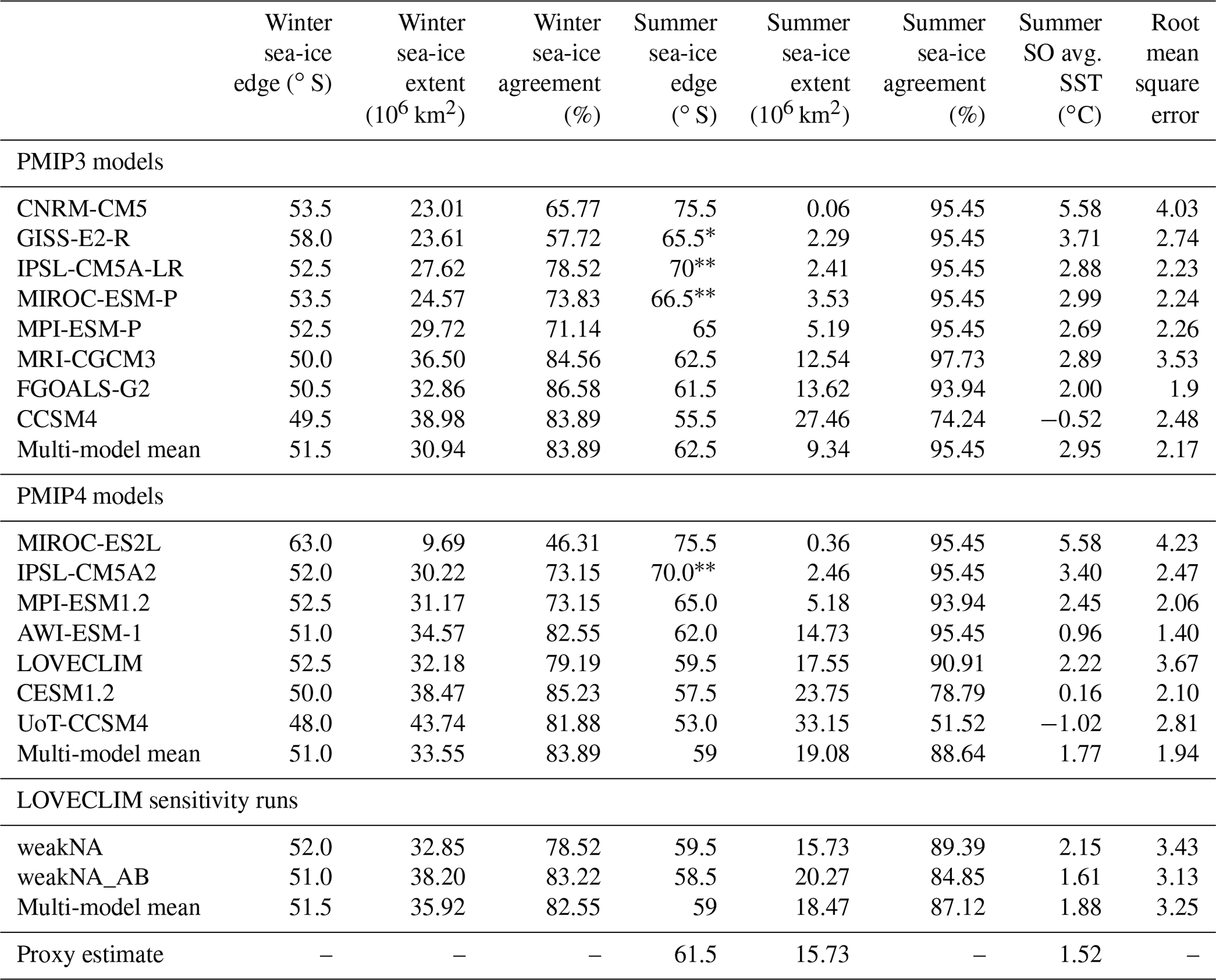
^∗ Models with sea-ice edge calculated only in the Ross Sea (150–220^∘ E). ${}^{\ast \ast }$ Models with sea-ice edge calculated only in the Ross (150–220^∘ E) and Weddell Seas (290–360^∘ E).

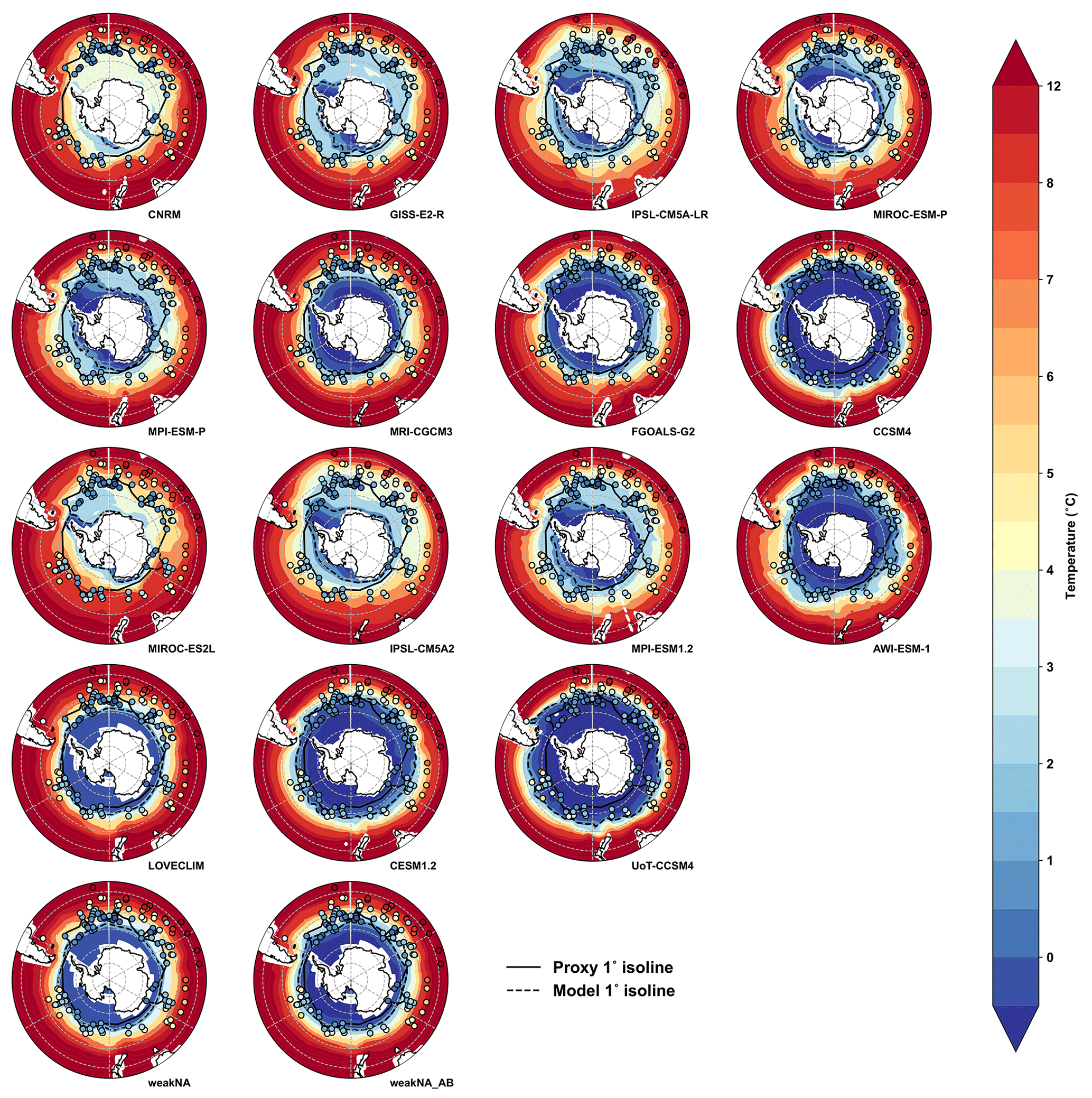
Figure 3 PMIP3, PMIP4 and LOVECLIM austral summer SST (shading) with SST proxy data overlain (filled circles). Fill color inside each SST reconstruction data point represents paleo SSTs at each location. Each model's 1 ^∘C isoline (dotted black line) is compared to the proxy SST data 1 ^∘C isoline (solid black line).

To look more closely into the regional distribution of SSTs, we plot each model's SO SST overlaid with the available SST data (Fig. 3). Due to biological limitations, diatom transfer functions are mostly available in regions with low sea-ice cover. As such, our proxy summer SST compilation only contains two locations with SST temperatures below 0 ^∘C. With limited proxy SST data near the freezing point, we instead assess the model data fit at the 1^∘ isoline. We therefore compute the 1 ^∘C isoline based on the proxies (solid black line in Fig. 3), and compare it to each model's 1 ^∘C isoline (dotted black line in Fig. 3). The proxy data are regionally variable, with lower temperatures (darker blue filled circles) in the Atlantic and Pacific sectors and higher temperatures (lighter blue, yellow, and red filled circles) in the Indian sector. Additionally, there are more records at lower latitudes in the Atlantic and Indian sectors. Figure 3 confirms that certain models are too warm (CNRM-CM5; GISS-E2-R; MIROC-ESM-P and MIROC-ES2L; IPSL-CM5A-LR and IPSL-CM5A2) and certain models are too cold (CCSM4 and UoT-CCSM4; CESM1.2). The models that simulate a 1 ^∘C isoline in good agreement with the proxy records are FGOALS-G2, AWI-ESM-1 and all LOVECLIM experiments (weakNA, weakNA_AB, LOVECLIM). To quantitatively establish how well the models simulate the SST proxy record, we calculate the root-mean-squared error (RMSE) between simulated SSTs and observations (Table 3). The model with the lowest RMSE value (1.40), representing the model for which simulated SSTs fit the reconstructions best, is the AWI-ESM-1 model. FGOALS-G2 also has a low RMSE value with 1.90.

Taking into account the spatial pattern of the sea-ice proxy record (Fig. 1), the regional variability of the SST proxy record (Figs. 2 and 3), and the RMSE scores from the SST proxy records (Table 3), the most likely LGM SSI edge lies at 61–62^∘ S, with a mean sea-ice extent of 14–15×10⁶ km², similar to the ones simulated by the AWI-ESM-1 or FGOALS-G2.

With such large SSI discrepancies among the models, we next look at the potential reasons for the observed intermodel spread. To identify drivers of intermodel sea-ice variability we analyze the thermodynamic and dynamic controls on sea-ice extent, as ocean temperatures exert a significant control on sea-ice formation and melt, and wind stress affects sea-ice transport.

3.4 Drivers of inter-model variability

The strength and location of the southern hemispheric westerly and polar easterly winds impact SO circulation, sea-ice transport and therefore sea-ice distribution (Purich et al., 2016; Holland and Kwok, 2012). On the other hand, the presence or absence of sea-ice also has a direct influence on surface winds (Kidston et al., 2011; Sime et al., 2016). Here, we focus on the influence of winds on sea-ice through the divergence created by the wind stress curl. Within the SO, divergence leads to upwelling of relatively warm circumpolar deep waters and thus heat loss to the atmosphere. This upwelling can therefore also impact SO sea-ice distribution. While the latitudinal position and magnitude of southern hemispheric westerlies at the LGM is poorly constrained (Kohfeld et al., 2013; Sime et al., 2016), we want to assess the impact of the simulated wind stress curl on ocean dynamics in each model. We thus use the wind stress outputs to estimate the location and strength of the SO upwelling, and its potential impact on sea-ice cover.

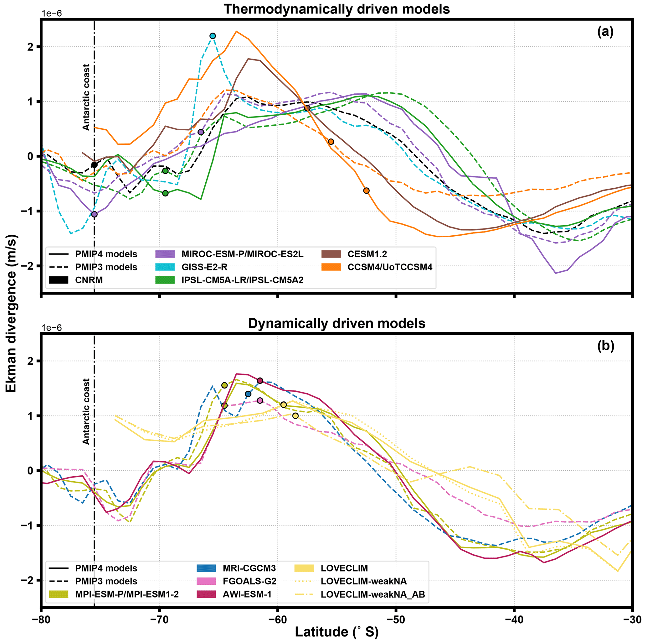
Figure 4 Zonally averaged austral summer Ekman divergence vs. latitude for (a) models in which mean temperature controls the summer sea-ice edge, (b) models in which Southern Ocean upwelling, and associated divergence, impacts the summer sea-ice edge. Each model’s sea-ice edge is represented with a filled circle.

Figure 4 shows the zonally averaged austral summer Ekman divergence in the SO with each model's sea-ice edge overlaid. Figure 4b shows LGM experiments in which the SSI edge falls within 2–3^∘ of their zonal mean Ekman divergence peak, indicating that sustained upwelling at 58–65^∘ S in these four models (MPI, FGOALS, AWI, LOVECLIM) most likely impacts summer SST and sea-ice cover. Our analysis suggests that the SSI edge in the MRI-CGCM3 LGM simulation is dynamically driven as its mean SO SST is close to the PMIP3 MMM, and its SSI edge is close to the maximum of the Ekman divergence. However, this result should be interpreted with caution as in the MRI-CGCM3 simulation the coupling between sea-ice and wind stress at the ice/atmosphere interface was absent due to a model bug (Marzocchi and Jansen, 2017).

On the other hand, Fig. 4a shows LGM experiments in which the SSI edge is more than 3^∘ away from the peak of the Ekman divergence. The models displayed in Fig. 4a both include LGM experiments with particularly high (CNRM-CM5, black; GISS-E2-R, cyan; MIROC-ESM-P and MIROC-ES2L, purple; IPSL-CM5A-LR and IPSL-CM5A2, green), and low (CCSM4 and UoT-CCSM4, orange; CESM1.2, brown) SST as identified in Sect. 2. While the sea-ice edge in GISS-E2-R seems to occur at the maximum of the Ekman divergence (cyan dotted line in Fig. 4a), this is an artifact of the averaging. This model's sea-ice edge is calculated only based on sea-ice in the Ross Sea due to the lack of sea-ice elsewhere. Therefore, the true global average sea-ice edge of GISS-E2-R at 15 % concentration is at the Antarctic coast, which is more than 3^∘ from its Ekman divergence peak. Divergence due to wind stress curl thus does not seem to have a large impact on SSI extent within the nine experiments (six models) shown in Fig. 4a.

We thus suggest that the location of the SSI edge in experiments displayed in Fig. 4a is thermodynamically controlled, whereas it is dynamically controlled for the ones displayed in Fig. 4b. It is interesting to note that experiments performed by the same models, or different versions of the same models, fall within the same categories, i.e., both PMIP3 and PMIP4 IPSL and MIROC experiments, as well as CCSM4 and UoTCCSM4 seem to be thermodynamically driven, whereas both PMIP3 and PMIP4 MPI and all LOVECLIM experiments seem to be dynamically driven.

As highlighted in Fig. 2, we find a clear relationship between seasonal sea-ice extent and seasonal SST. Additionally, as surface processes impact temperatures at deeper layers, we also find a statistically significant relationship between SO temperature (defined as the ocean temperature zonally averaged between 50 and 75^∘ S over the whole water column) and both WSI and SSI extent (Fig. 5). The larger the sea-ice extent, the lower the SO SST, and thus the lower the mean SO temperature. However, SO temperature is only partly controlled by AABW temperature but also by the latitudinal extent and temperature of circumpolar deep waters. For example, while they display very different sea-ice covers, both CCSM4 and GISS-E2-R simulate AABW close to freezing. However, in the GISS-E2-R simulation, the AABW extent is limited and the relatively warm NADW leads to warm circumpolar deep waters (Fig. 6).

The interplay between SO surface conditions and seasonal sea-ice cover modulates AABW temperature. LGM experiments with relatively cold surface conditions and relatively large SSI cover (e.g., CCSM4, LOVECLIM) also simulate cold ($<-\mathrm{1}$ ^∘C) AABW. On the other hand, some LGM experiments with relatively warm conditions still simulate cold AABW due to the large seasonal difference in sea-ice cover (GISS-E2-R, MIROC-ESM-P). Finally, LGM experiments with both warm surface SO conditions and low seasonal differences in sea-ice cover simulate anomalously warm AABW (CNRM-CM5, MIROC-ES2L).

4 Discussion and conclusions

We suggest that during the LGM, the likely austral WSI edge was between 50.5 and 51.5^∘ S, with a mean sea-ice extent of 35–36×10⁶ km². During austral summer we suggest the sea-ice edge was likely between 61 and 62^∘ S, with a mean sea-ice extent of 14–15×10⁶ km², similar to the sea-ice characteristics simulated by AWI-ESM-1 and FGOALS-G2. This is an improved constraint on LGM SSI extent as we combine modeling results with paleo-estimates of sea-ice cover and summer SST data. Previous LGM estimates, which were based only on sea-ice proxy data, are lower than ours (10.2–11.1×10⁶ km²) (Lhardy et al., 2021; Roche et al., 2012). Our estimates can also be compared to the average modern austral WSI extent of 18.5×10⁶ km² and the average modern austral SSI extent of 3.1×10⁶ km² (Eayrs et al., 2019).

Our estimate for the LGM SSI edge is a zonal average and therefore assumes a fairly circular SSI distribution, similar to that simulated by AWI-ESM-1 and FGOALS-G2 (Fig. 1). While the LGM SSI proxy data are limited, Lhardy et al. (2021) suggest that the three basins behaved very differently, with a LGM SSI edge at 54^∘ S in the Atlantic, 65–66^∘ S in the Indian, 63^∘ S in the western Pacific and 66–68^∘ S in the eastern Pacific. If this indeed was the case, our suggested LGM SSI edge would potentially overestimate the sea-ice edge in some regions while potentially underestimating it in other regions. Additional proxy data from the Pacific and Indian basins would reduce the uncertainty of our estimate.

While the SSI edge is thermodynamically driven for six of the models considered here, it is linked to the position of the maximum wind stress curl for the remaining five models (Fig. 4). The maximum wind stress curl corresponds to the maximum Ekman transport divergence, leading to deep-water upwelling. This can impact sea-ice both thermodynamically and dynamically, as upwelling is often linked with ocean heat release, while the Ekman transport divergence can lead to strong equatorward transport of sea-ice. Given the uncertainties that surround the magnitude and position of the Southern Hemisphere westerlies at the LGM (e.g., Kohfeld et al., 2013; Sime et al., 2016), this casts additional uncertainties on the location of the austral SSI edge. Furthermore, paleo records of austral SSI extent used here are mostly restricted to 40–60^∘ S, with 95 % of the records suggesting ice-free conditions. Due to this, they can only provide an estimate of the maximum SSI extent. Additional proxy records recovered from locations south of 60^∘ S are thus needed to better constrain the SSI extent.

Figure 5 Scatter plots showing the relationship between sea-ice, SO SST (averaged over 50–75^∘ S) and SO temperature (averaged over 50–75^∘ S and 0–5500 m depth) in all experiments. Panels (a) and (b) show the relationship for austral summer and panels (c) and (d) show the relationship for austral winter.

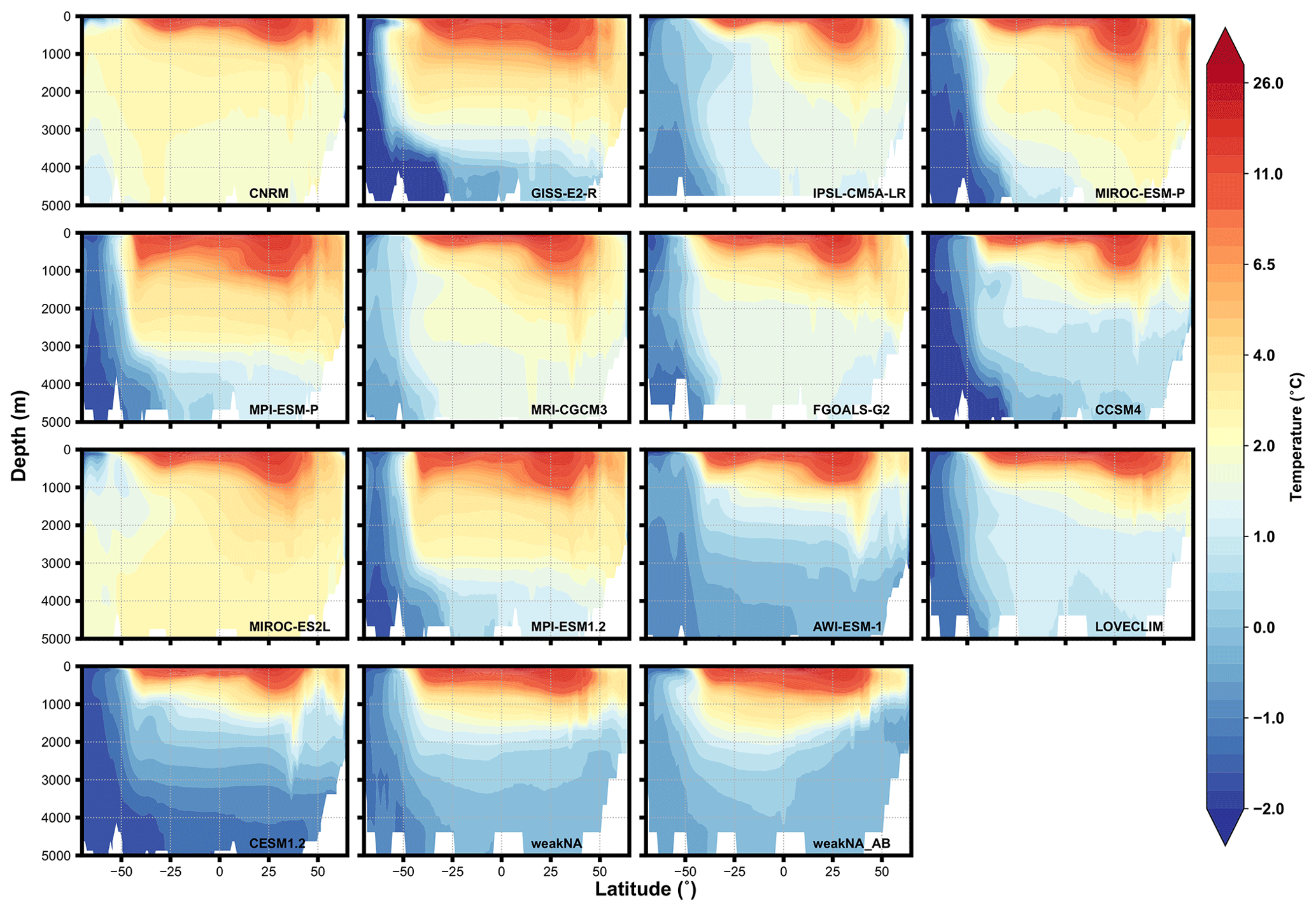
Figure 6 Zonally averaged oceanic potential temperatures (^∘C) in the Atlantic basin for PMIP3, PMIP4 and LOVECLIM simulations.

Both the PMIP4 and PMIP3 experiments display a relatively large range ($\sim -\mathrm{2}$ to 4 ^∘C) of temperatures in the deep Atlantic Ocean (Fig. 6). Only a few paleo records of deep ocean temperature are available for the LGM, but they suggest ocean temperatures below 0 ^∘C throughout the deep Atlantic (Adkins et al., 2002). In the southwest Pacific at ODP Site 1123, $\mathrm{Mg}/\mathrm{Ca}$ records find deep ocean temperatures of −1.1±0.3 ^∘C at the LGM (Elderfield et al., 2010). The models that simulate warm SO conditions with little sea-ice also simulate a warm bias at depth, even though in some cases a large seasonal ($\sim \mathrm{20}\times {\mathrm{10}}^{\mathrm{6}}$ km²) difference between maximum and minimum sea-ice extent can lead to cooler abyssal temperatures.

In this study, we also included three LGM experiments performed with the earth system model LOVECLIM. The oceanic circulation was varied in two of these experiments by adding meltwater in the North Atlantic and SO and weakening the southern hemispheric westerly wind stress (Menviel et al., 2017). Despite significant differences in oceanic circulation in these three simulations, with weaker AABW transport in weakNA_AB compared to weakNA, and weaker Atlantic meridional overturning circulation (AMOC) in weakNA (14.7 Sv) and weakNA_AB (11.2 Sv) compared to the PMIP4 LOVECLIM experiment (26 Sv), the differences in sea-ice extent between these three experiments are much smaller than the intermodel differences between all PMIP3 and PMIP4 simulations. This indicates the limitations of performing model data comparisons with a single model to infer SO climatic conditions.

We further assess the relationship between LGM SSI and AMOC strength (Fig. S2, Muglia and Schmittner, 2015; Kageyama et al., 2021), and find that there is no statistically significant relationship between the two (R²=0.04). There is, however, a weak relationship between SSI extent and AMOC depth (Fig. S2, R²=0.17), with a shallower AMOC generally associated with a larger SSI extent. A larger SSI extent, and thus increased sea-ice formation, could impact the AABW properties and therefore ocean stratification (Marzocchi and Jansen, 2017), as evident from Fig. 6. However, climatic conditions in the North Atlantic are probably the principal driver of AMOC depth (Oka et al., 2012; Muglia and Schmittner, 2015). There is also no link between the equilibrium climate sensitivity (ECS) of these models and their austral SSI cover, with the three models displaying the least amount of sea-ice exhibiting ECS of 3.3 ^∘C for CNRM-CM5, 2.7 ^∘C for MIROC-ES2L, and 2.1 ^∘C for GISS-E2-R, while the two models with the most sea-ice have an ECS of 2.9 ^∘C and 3.2 (CCSM4 and UoT-CCSM4, respectively, Kageyama et al., 2021).

Based on our best estimates of LGM WSI and SSI cover over the SO, the seasonal variation in the sea-ice edge is ∼10^∘ and the seasonal variation in sea-ice extent is 20–22×10⁶ km². In comparison, the present day seasonal change in sea-ice edge ranges from ∼15^∘ in the Atlantic sector to less than 5^∘ in the Indian sector (Cavalieri and Parkinson, 2012). The present day seasonal variation in sea-ice extent is $\sim \mathrm{15.4}\times {\mathrm{10}}^{\mathrm{6}}$ km² (Eayrs et al., 2019), thus indicating a larger sea-ice seasonality during the LGM. Such a large sea-ice seasonality would in turn impact SO dynamics through changes in buoyancy (Marzocchi and Jansen, 2017) as well as the carbon cycle (Haumann et al., 2016). While a large year-round LGM sea-ice cover could contribute to a lower atmospheric CO₂ concentration (Ferrari et al., 2014), the impact of a large sea-ice seasonality on the carbon cycle is not well constrained. The increased seasonality has potential to dampen CO₂ drawdown, depending on the balance between upwelling and subsequent outgassing of carbon-rich deep waters and nutrient utilization at the surface (e.g., Menviel et al., 2008). Conversely, the increased seasonality could also amplify carbon drawdown through enhanced brine formation, increasing the density gradient between the surface and deep waters (Galbraith and de Lavergne, 2019), and potentially lowering atmospheric CO₂ (Bouttes et al., 2012). Despite proxy records showing lower productivity in the Antarctic Zone (Jaccard et al., 2013), increased stratification due to sea-ice melt during spring-summer could enhance nutrient utilization and thus carbon drawdown (Sigman and Boyle, 2000; Abelmann et al., 2015). While some studies have suggested a primary role for LGM sea-ice cover in driving changes in oceanic carbon content (Ferrari et al., 2014), the LOVECLIM experiments presented here have also shown that reduced ventilation of the deep ocean through weaker AABW transport could instead be the primary driver of an increase in deep ocean carbon content (Menviel et al., 2017).

Antarctic sea-ice integrates oceanic and atmospheric processes occurring at high southern latitudes, and can also significantly impact Antarctic climate (Bracegirdle et al., 2015). Sea-ice has the ability to protect ice-shelves (Massom et al., 2018) and floating ice-shelves play a significant role in buttressing Antarctic outlet glaciers (Scambos et al., 2004). It is thus crucial that models incorporate a good representation of preindustrial and present day sea-ice, but also manage to correctly simulate past sea-ice extent during both cold periods, such as the LGM, and warm periods such as the Last Interglacial (125 000 years ago). In that respect, it is interesting to note that the models which underestimate austral summer Antarctic sea-ice cover at the LGM also underestimate the austral SSI cover under preindustrial conditions, while the model simulating the largest LGM sea-ice cover also overestimates the preindustrial SSI cover (Marzocchi and Jansen, 2017; Goosse et al., 2013; Roche et al., 2012). This implies that targeting a good agreement between model and observations for present day climate should remain a priority.

In this study, we have analyzed SO WSI and SSI cover in LGM simulations and compared the outputs against available proxy reconstructions. In doing so, we identify the potential drivers for intermodel SO sea-ice differences, in addition to placing improved constraints on the LGM SO SSI and WSI extents. This improved understanding of sea-ice dynamics can provide valuable information about the earth's system and important insights into the strengths and weaknesses of models currently used.