the Creative Commons Attribution 4.0 License.
the Creative Commons Attribution 4.0 License.
 | 19 Apr 2022
crestr: an R package to perform probabilistic climate reconstructions from palaeoecological datasets
Manuel Chevalier
Statistical climate reconstruction techniques are fundamental tools to study past climate variability from fossil proxy data. In particular, the methods based on probability density functions (or PDFs) can be used in various environments and with different climate proxies because they rely on elementary calibration data (i.e. modern geolocalised presence data). However, the difficulty of accessing and curating these calibration data and the complexity of interpreting probabilistic results have often limited their use in palaeoclimatological studies. Here, I introduce a new R package (crestr) to apply the PDF-based method CREST (Climate REconstruction SofTware) on diverse palaeoecological datasets and address these problems. crestr includes a globally curated calibration dataset for six common climate proxies (i.e. plants, beetles, chironomids, rodents, foraminifera, and dinoflagellate cysts) associated with an extensive range of climate variables (20 terrestrial and 19 marine variables) that enables its use in most terrestrial and marine environments. Private data collections can also be used instead of, or in combination with, the provided calibration dataset. The package includes a suite of graphical diagnostic tools to represent the data at each step of the reconstruction process and provide insights into the effect of the different modelling assumptions and external factors that underlie a reconstruction. With this R package, the CREST method can now be used in a scriptable environment and thus be more easily integrated with existing workflows. It is hoped that crestr will be used to produce the much-needed quantified climate reconstructions from the many regions where they are currently lacking, despite the availability of suitable fossil records. To support this development, the use of the package is illustrated with a step-by-step replication of a 790 000-year-long mean annual temperature reconstruction based on a pollen record from southeastern Africa.
- Article
(7212 KB) - Full-text XML
-
Supplement
(74 KB) - BibTeX
- EndNote


Fossil-based climate reconstruction techniques are commonly used to quantify past climates and shed light on the nature of the drivers of climate change across space and time. Over the years, numerous techniques of increasing complexity have been proposed, each one based on a unique set of assumptions regarding the modelling of (palaeo)ecological datasets and their translation into climate reconstructions (e.g. Birks et al., 2010; Chevalier et al., 2020b). In particular, many techniques focus on modelling the relationships between proxy assemblages and climate from collections of modern proxy samples. Of these techniques, weighted averaging (WA, ter Braak and van Dame, 1989), weighted-averaging partial least square (WA-PLS, ter Braak and Juggins, 1993), and the modern analogue technique (MAT, Hutson, 1978; Overpeck et al., 1985) have been the most widely employed because of their conceptual simplicity, their demonstrated capacity to reconstruct climate from various palaeoecological proxies (e.g. fossil pollen, chironomids, foraminifera) and their accessibility via multiple software tools. However, the limited availability of the necessary calibration datasets beyond the Northern Hemisphere extratropics has often hindered their application in many environments and regions where quantified climate reconstructions are needed, despite the existence of suitable fossil records (Chevalier et al., 2020b).
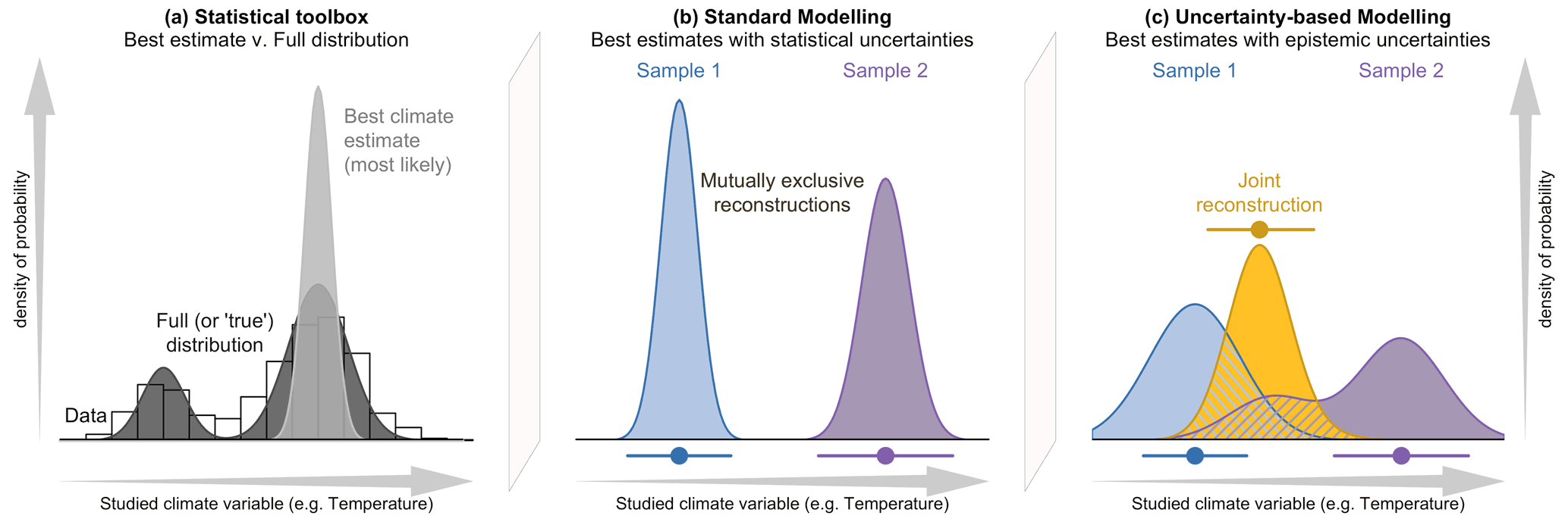
Figure 1(a) Conceptual illustration of the differences between a modelling approach based on the full spread of the data with the probabilities spread along the climate gradient (e.g. CREST; dark grey), and a modelling approach focused on the estimation of the “most likely” or “best” climate value with small statistical errors surrounding it (e.g. MAT or WA-PLS; light grey). In both cases, the area under the curve sums to one. The results of the two types of approaches are illustrated in (b, c), where two theoretical fossil assemblages (in blue and purple) are used to produce two independent reconstructions of the same climatic parameter for the same time interval. (b) The two reconstructions are derived from a method that only estimates the most likely climate value, resulting in “apparently” incompatible reconstructions. (c) The same fossil assemblages are analysed using an approach that estimates their complete uncertainty distributions. In this case, the blue reconstruction is broader, and the purple reconstruction becomes bimodal. When the full spread of these uncertainties is considered, the two reconstructions are not incompatible anymore, and a joint climate estimate (gold) can be derived from their overlapping sections (hashed polygons).
In contrast, the “indicator species” family of reconstruction techniques uses modern proxy occurrences (i.e. collections of locations where the studied proxy species can be observed in modern environments) to estimate individual proxy–climate relationships (Chevalier et al., 2020b). Because such occurrence data are generally easier to obtain than modern proxy assemblages, this fundamental difference implies that indicator species methods can contribute to filling in the reconstruction gaps that exist at the global scale. The CREST (Climate REconstruction SofTware) technique is a probabilistic indicator species method initially developed to produce quantified climate reconstructions from southern African pollen records (Chevalier et al., 2014). Derived from the original work of Kühl et al. (2002) – who first proposed to replace the commonly used modern proxy assemblages with modern geolocalised occurrence data to estimate probabilistic proxy–climate relationships for palaeoclimatic studies – CREST estimates and combines probabilistic proxy–climate relationships to reconstruct past climate parameters from fossil proxy observations. Built on a private collection of modern plant occurrences held by the South African National Botanical Institute (SANBI), CREST was first employed to reconstruct diverse temperature, precipitation and moisture-related variables for different time intervals across the southern African drylands (see for instance Chase et al., 2015b, a; Chevalier and Chase, 2015, 2016; Lim et al., 2016; Cordova et al., 2017).
Since the assumptions of CREST do not restrict its use to southern African pollen records, CREST was also integrated into a point-and-click graphical user interface to enable its use by the broader community (Chevalier et al., 2014). However, the complexity of collating and formatting the thousands of distinct occurrences required to estimate reliable proxy–climate relationships limited its practical use. To overcome this limitation, a global, multi-proxy calibration dataset containing millions of modern occurrence data for plants, beetles, chironomids, foraminifera, and diatoms was subsequently released (Chevalier, 2019), and this curated dataset contributed to creating quantified climate reconstructions beyond southern Africa (e.g. Yi et al., 2020; Hui et al., 2021; Gibson et al., 2022). However, maintaining the compatibility of the graphical interface across a range of constantly evolving operating platforms has been challenging. This paper thus introduces a new multi-platform R package crestr designed to replace the original interface. crestr integrates the global calibration dataset and provides simple solutions to tailor it to the users' specific needs. The package also proposes an array of graphical diagnostic tools to represent the calibration and reconstruction data at different pivotal steps of the reconstruction process and thus facilitate data and result interpretations.
In addition, the advantage of using CREST is not limited to its capacity to produce quantified reconstructions in understudied regions. CREST is equipped with some fundamental statistical features that make it well-adapted to analysing extensive collections of palaeoecological records from any region (Chevalier et al., 2020b). While techniques such as MAT or WA-PLS are primarily designed to associate modern proxy observations with their “most likely” or “mean” climate values only, CREST estimates and weighs all the climate values that are compatible with the observed fossil data. As such, the application of CREST yields a probabilistic quantification of all the climate values that are compatible with the studied data instead of simpler, less informative “most likely” or “best” climate estimates. While the “best estimate” approach might be optimal when a fossil assemblage is analysed in complete isolation, the presence of independent – local or regional – information (e.g. other reconstructions from the same core or independent records) usually provides additional information that may not always be consistent with the best estimate reconstructions (see Fig. 1). In practice, joint solutions based on all the available information often differ from best climate estimates. Using methods such as CREST that can estimate the full range of climate uncertainties associated with a proxy sample is thus critical to bring reconstructions and even climate simulations together in a cohesive way.
This article introduces the crestr R package and provides good-practice recommendations to produce high-quality climate reconstructions. The article is structured as follows: Sect. 2 summarises the most important mathematics and assumptions underlying the approach. Understanding all the details of this section is not necessary to use the package. Then, Sect. 3 describes the embedded calibration dataset, how it was built and how the data are structured. Section 4 explains the philosophy and main elements of the package and describes the format of the different input files required. Finally, Sect. 5 documents a step-by-step guided tour of the package, illustrating the successive stages of a CREST analysis and how to use the diagnostic tools to reproduce a recently published pollen-based temperature reconstruction (Chevalier et al., 2021a).
The core process of a CREST reconstruction can be decomposed into two successive stages: (1) modelling the proxy–climate responses of the proxies observed in the fossil sequence by correlating modern occurrence data with corresponding climate values (Fig. 2) and (2) reconstructing past climate by combining these responses based on the information provided by the fossil data. This section presents the most important details of these two stages and details the parameters and modelling assumptions that can be modified in crestr. Readers interested in an in-depth description or discussion of the method and its modelling assumptions are referred to Chevalier et al. (2014, 2020b).
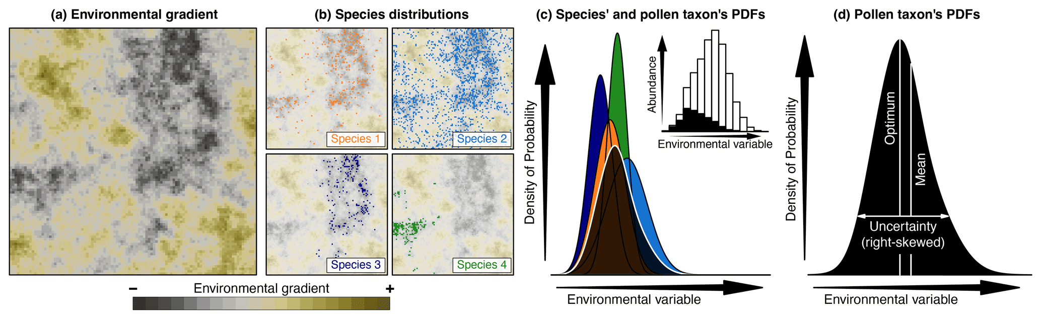
Figure 2Conceptual representation of CREST illustrated with artificial pollen data. (a) Modern distribution of a climate variable to reconstruct (e.g. temperature). (b) Occurrences of four species part of the same pollen morphotype exhibiting marked preferences for the lowest values of that climate (e.g. dark/cold values) across the study area. (c) Combination of the four species PDFs (in colour) and the resulting pollen taxon PDF (in black). The histogram in the inset panel represents the proportion of the modern climate space (white) occupied by at least one of the four species (black), highlighting the higher chances of observing the taxon at the lower end of the climate gradient. (d) Taxon PDF derived from the combination of the four species PDFs and the type of synthetic statistics (e.g. optimum, mean, uncertainty range) that can be derived from it. While the shape of the species PDFs is constrained, taxon PDFs can be irregular, skewed and even multi-modal.
2.1 Nature of the required data
Three types of data are required to reconstruct climate parameters with the CREST method:
-
a fossil proxy record with several taxa being co-recorded and expressed as counts, percentages or binary presence/absence;
-
modern presence-only occurrence data of species corresponding to the taxa observed in the fossil record (i.e. collections of geographical coordinates where the species are observed across a user-defined study area; see Fig. 2b and Sect. 3 for an example of a curated dataset);
-
climatology(ies) of the variable(s) to reconstruct gridded at the same resolution as the modern occurrences (Fig. 2a). All the climate values observed in the study area define the climate space.
2.2 Modelling the proxy–climate relationships
CREST takes into account that some fossil taxa can be identified at the species level (e.g. plant macrofossils), while others are only identified at a lower taxonomic resolution (e.g. fossil pollen are commonly identified at the genus, sub-family, or even family level; Chevalier et al., 2020b). The transformation of the information contained in the modern observations of the biological climate proxies into probabilistic climate responses is thus done in one or two steps depending on the taxonomic resolution of the studied proxy. However, determining a list of species that could have produced that fossil is necessary when the observed fossil taxa are not identified at the species level. The way to make this species to fossil proxy association is described in Sect. 4.3.2.
The individual climate responses of all the species identified are estimated as univariate probability density functions (PDFs) for every climate variable. Because CREST aims to be applicable even in data-sparse environments, the estimation of these responses is based on simple assumptions that exclude using complex algorithms, such as those described in, for instance, the recent review of Valavi et al. (2021). The species' individual responses for climate variable c are derived from the empirical mean () and associated variance () of all the Ns climate values (cs,i, where ) where species s is observed:
where k(cs,i) is a weighting parameter that can be used to account for the uneven distribution of climate in modern environments (Kühl et al., 2002; Bray et al., 2006). This correction takes into account that extreme values are usually under-represented in the climate space (see, for instance, the white inset histogram in Fig. 2c), which “pushes” the peak of the PDFsp(c,s) towards the mean climate observed across the study area (i.e. towards the centre of the climate space). It can also artificially shrink the range of the reconstructions. Here, the weights are calculated by first sorting the N climate values that compose the modern climate space into bins of equal width (e.g. 2 ∘C or 50 mm). Then, each climate value cj () is given a weight k(cj) defined as the inverse of the number of values that belong to same bin :
With this correction, the most abundant climate values in the climate space are down-weighted, and the rarer ones are up-weighted so that the distribution of modern climate is overall more “balanced”. The two parameters and ss,c can be interpreted as the climate preference and tolerance of the species, respectively. For a reliable estimation, excluding species with few observations is recommended. Different studies have shown that a threshold of a minimum of Ns≥20–25 distinct occurrences usually leads to reliable estimates (e.g. Chevalier et al., 2014, 2021a). However, this number can vary between regions and proxies.
Once estimated, and are used to define a regular, unimodal PDFsp(s,c) for species s and climate variable c. Here, we assume that the shape of these species responses should be unimodal and can be either normal:
or log-normal if the variable is not defined for negative values (e.g. precipitation variables):
For the fossil taxa t that are not identified at the species level, the PDFsp(c,s) of their S(t) composing species are combined together to meet the taxonomic resolution of the fossil observation (hereafter PDFtx(t,c)):
This linear combination ensures that all the climate values that support the presence of at least one species have a non-null probability in the PDFtx(t,c). Contrary to the previous step, no additional constraints are added here. The distribution of the PDFtx(t,c) can thus be asymmetrical and even multimodal if different (groups of) composing species exhibit distinct climate requirements. An additional option is to weigh the different PDFsp(s,c) by the square root of the number of individual occurrences composing their distribution (Ns). Considering that it is more difficult to estimate robust parameters with few points, this weighting gives more importance to the species with more extensive geographical distributions today. Said differently, it gives more weight to the species whose climate responses can be the most reliably defined.
Finally, it is important to note that if a fossil taxon is taxonomically resolved at the species level, its number of composing species S(t) equals 1. The resulting PDFtx(t,c) is thus equivalent to its PDFsp(s,c). A fossil sample can thus be composed of a mix of taxa identified at the species level and taxa identified at a lower taxonomical level without interfering with the reconstruction algorithm.
2.3 Reconstructing climate
Climate c is reconstructed from fossil sample z (itself associated with a unique age, depth or any other identifier) by multiplying the PDFtx(t,c) of the T(z) selected taxa:
where ω(t,z) is a positive value that is used to weigh taxon t in sample z. For presence/absence observations, the weights ω(t,z) of taxon t will be either one (the taxon is observed) or zero (the taxon is not observed and does not influence the reconstruction). For compositional data, ω(t,z) can be the observed percentages (i.e. values between 0 and 100). However, using raw percentages implies that the observed percentages are directly proportional to the taxa composition across the catchment. This can give considerable weight to abundant, ubiquitous taxa that do not necessarily have a well-defined climate response and, in contrast, can strongly limit the influence of rarer taxa with stricter climate preferences. An empirical normalisation is proposed in CREST to account for the varying production rates, distribution and preservation processes impacting the relative proportions of taxa observed in the sediments (Chevalier et al., 2014). In this taxon-specific scaling method, the percentages of each taxon are divided by their average percentage when it is present (zeros are excluded from the calculation of the average):
where O(t,z) represents the observed percentage of taxon t in sample z. With this transformation, all the normalised percentages vary on a standardised scale. The average presence is given a weight of 1, and values below and above this average presence threshold are assumed to represent lower and higher abundance in the environment, respectively. While the empirical nature of this solution makes it imperfect and sensitive to the quality of the data, it nevertheless enables using percentages to inform the reconstructions. The three weighting options described here are available in crestr, but users can also design their own weights to better account for the specificity of their data.
Finally, the presence of each taxon in a sample is considered independent from the others. It is thus possible to select a subset of sensitive taxa to reconstruct a specific climate variable. In some cases, identifying a subgroup of climate-sensitive taxa can help disentangle the different climate signals represented by the palaeoecological data and improve the quality of the reconstructions (Chevalier and Chase, 2015), even if it is not always necessary (Chevalier et al., 2021a). These choices should be dictated by the data themselves and the users' understanding of the studied proxy system. crestr provides graphical tools to help identify the possible climate sensitivities of the studied taxa across the study area (Chevalier et al., 2021b).
A multiproxy calibration dataset to estimate PDFs from a global collection of presence-only occurrence data (hereafter proxy “distributions”) was introduced in Chevalier (2019). These data were obtained from the Global Biodiversity Information Facility (GBIF) database, an online collection of geolocalised observations of biological entities (GBIF, 2018). The calibration dataset (hereafter gbif4crest, Chevalier, 2020) contains the species distributions of six common palaeoecological fossils: the five taxa presented in the original version of the dataset – plants (GBIF, 2020l, h, k, f, g, m, i, n, j, 2021a, b) for fossil pollen and macrofossils, chironomids (GBIF, 2020b), beetles (GBIF, 2020a), diatoms (GBIF, 2020c) and foraminifera (GBIF, 2020d) – to which rodents (GBIF, 2020e) were recently added (Fig. 3). These data were curated and stored in a relational database to ensure the consistency of the data.
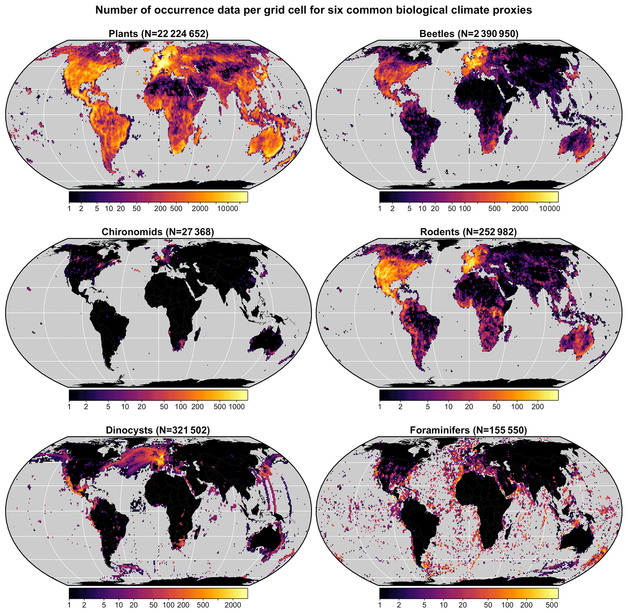
Figure 3Distribution and grid cell density of the six climate proxies available in the gbif4crest calibration database. The total number of unique species occurrences (N) is indicated for each proxy. The maps are based on the “Equal Earth” map projection to better account for the relative sizes of the different continents.

Figure 4Structure of the gbif4crest PostgreSQL database. By default, the package extracts data from the TAXA, DISTRIB-QDGC and DATA-QDGC tables. The DISTRIB table contains the raw occurrence data obtained from GBIF and can be used to curate the distribution data at a different spatial resolution. Note that the DATA-QDGC table spreads across two rows on this figure.
The coordinates of all the presence records of these six common
palaeoecological fossil proxies were mapped onto a grid with a spatial
resolution of (hereafter QDGC for
quarter-degree grid cell). The QDGC spatial resolution is an empirical
trade-off between numerous factors, including the resolution of the
presence data, the quality of the data or the spatial representativity
of the studied proxy (see discussions in Chevalier et al., 2014,
and Chevalier, 2019). However, this trade-off may be suboptimal in
some situations. For that reason, crestr can also be used with
the raw GBIF data (stored in the DISTRIB table, Fig. 4) and even independent calibration datasets.
In the gbif4crest database, all the QDGC grid cells were associated with a collection of terrestrial and oceanic environmental variables that can be reconstructed (Fick and Hijmans, 2017; Zomer et al., 2008; Locarnini et al., 2019; Zweng et al., 2018; Garcia et al., 2019a, b; Reynolds et al., 2007, see details in Tables 1 and 2). Despite the diversity of variables available, it is recommended to avoid serial reconstructions and, on the contrary, to identify the few important variables for the studied palaeoecological datasets a priori. The grid cells were also associated with “non-reconstructible” environmental and geographical descriptors that serve to tailor the calibration dataset to the users' needs. These include the coordinates, the elevation and elevation variability within the grid cell (Amante and Eakins, 2009), the country (https://www.naturalearthdata.com, last access: September 2021) or ocean (https://www.marineregions.org, last access: September 2021) names, as well as different levels of ecological classification for the terrestrial (Olson et al., 2001) and marine (Costello et al., 2017) realms.
Table 1List of terrestrial variables available for reconstruction in the gbif4crest database. Each one can be selected in crestr using its associated code. Temp – temperature, Precip. – precipitation.
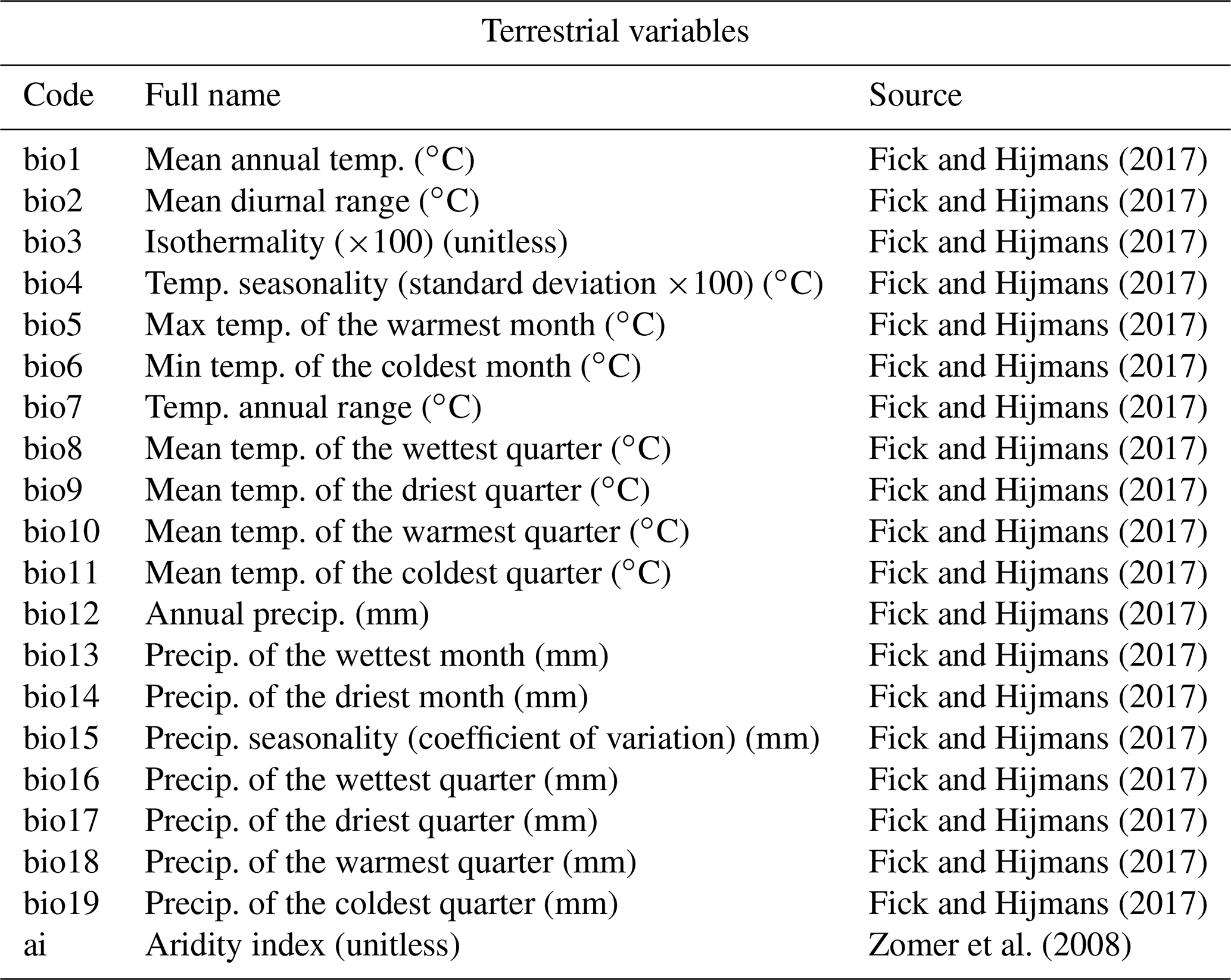
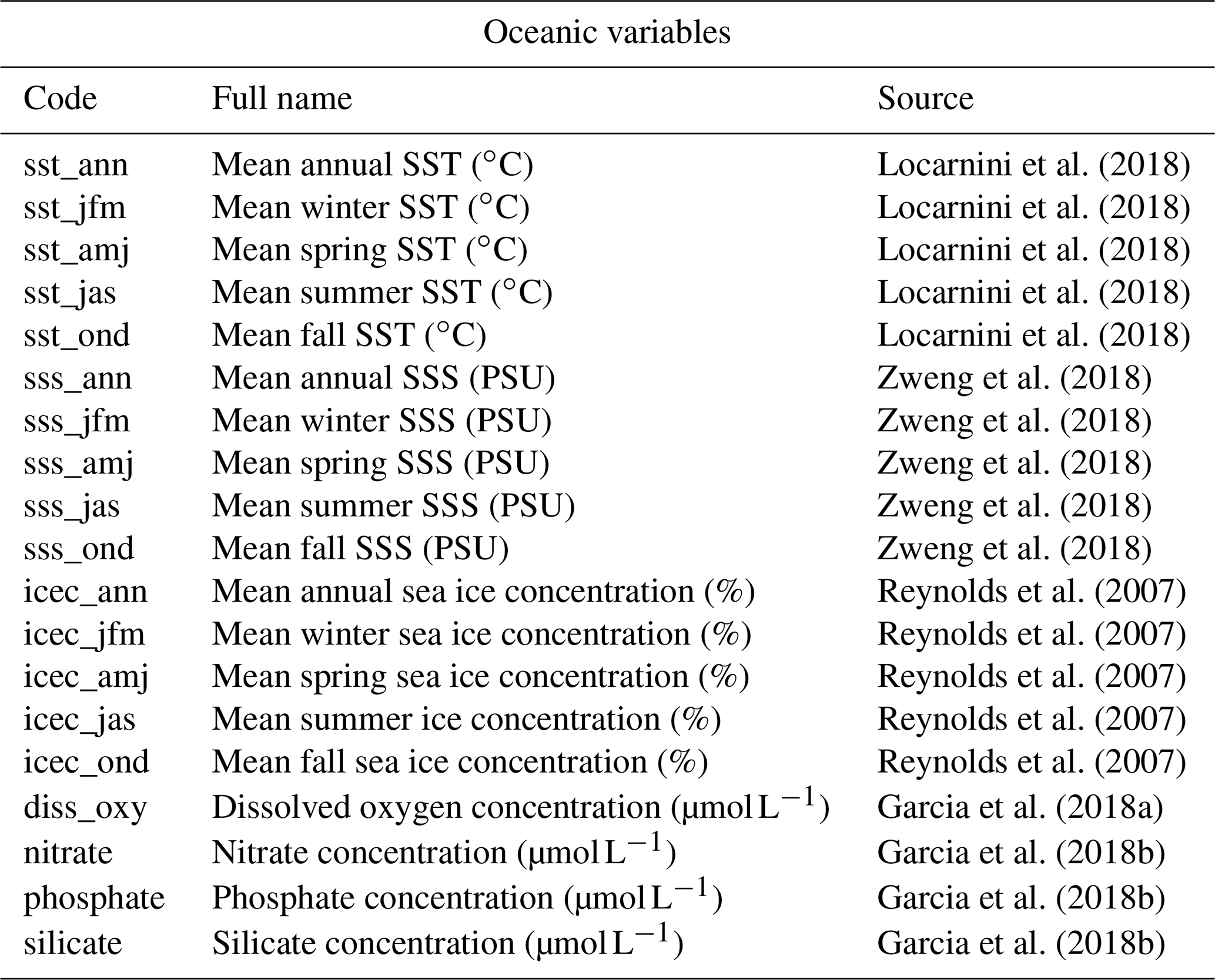
Table 2List of marine variables available for reconstruction in the gbif4crest database. Each one can be selected in crestr using its associated code. SST – sea surface temperature, SSS – sea surface salinity.
In its current version (V2), the gbif4crest calibration dataset contains about 25.3 million unique QDGC occurrence data for the six climate proxies. Unfortunately, the density of data available varies between proxies and regions (Fig. 3). Plant data largely dominate the calibration dataset (>22 million unique occurrences) and allow for the use of crestr across all landmasses. For the five other proxies, the calibration data are not as extensive. However, these datasets are regularly updated by GBIF. For example, the first version of the gbif4crest dataset released in 2018 contained about 17.5 million QDGC entries (∼44 % increase). The range of “reconstructible” areas is thus rapidly broadening (see, for instance, the coverage of Russia by plant data compared to the first version of the gbif4crest dataset presented in Chevalier, 2019). This database will be regularly updated, and specific requests can also be made.
The gbif4crest database is composed of three main types of data:
taxonomic data (TAXA table in Fig. 4),
distribution data (DISTRIB (raw data) and
DISTRIB_QDGC (curated data) tables) and diverse geopolitical,
climatological, and environmental data (DATA_QDGC table). Its
structure is slightly different from the first version presented in
Chevalier (2019), with a grouping of all the separate QDGC tables in a
unique DATA_QDGC table to enable faster data extraction. The
DISTRIB_QDGC tables link the TAXA and
DATA_QDGC tables using the unique identifiers taxonID
and locID, respectively. Each occurrence's first and last
observation dates are also now included, along with the type of
observation reported by GBIF (see
https://rs.gbif.org/vocabulary/dwc/basis_of_record.xml, last access: September 2021) and the number
of observations n_occ reported between the first and the last
observation dates. The DATA_QDGC table was also entirely
recalculated using a new protocol that better accounts for coastal
margins, implying that some coastal climate values may differ, however
marginally, between the different versions of the gbif4crest
dataset.
Due to its large size (about 15 Gb), this database is not downloaded
when installing the package but can be accessed through different
routes. First, the data are stored in an open-access, cloud-based
PostgreSQL database that can be accessed via crestr. This
solution is the recommended option, as users without any SQL knowledge
can benefit from the package's interface to automatically query the
database simply by providing study-specific parameters (e.g. the
name of the taxa or geographical boundaries for the study area) to
import all the necessary data in the correct format to the R environment
(see Sect. 5.2). Second, more advanced
users can also directly query the database to extract and curate data
from the DISTRIB or DISTRIB_QDGC tables using SQL
requests and the dbRequest() function. Finally, the full
gbif4crest calibration dataset can also be downloaded as an
SQLite3 portable database file from Chevalier (2020).
4.1 Philosophy of the package
The crestr package has been designed for two independent but complementary modelling purposes. The probabilistic proxy–climate responses can be used to quantitatively reconstruct climate from their statistical combination, such as in Chevalier et al. (2021a) or Chevalier and Chase (2015), or they can be used in a more qualitative way to determine the (relative) climate sensitivities of different taxa in a given area to characterise past ecological changes, such as in Chevalier et al. (2021b) or Quick et al. (2021). To simplify access to the functionalities, default values are provided for all parameters to enable a rapid generation of preliminary results that users can then use as a starting point to adapt the model to their data. Different publication-ready graphical diagnostic tools were designed to represent the CREST data in a standardised way to guide users in this task and avoid the typical “black box” criticism many complex statistical tools face. These tools include plots of the calibration data, the estimated climate responses, the reconstructions and more. These figures allow looking at the data from different perspectives to help interpret the results and possibly identify potential issues or biases in the selected data and parameters. Such diagnostic tools are available for every stage of the process, and, as exemplified in Sect. 5, they can be generated with a single line of R code.
4.2 The central element: the crestObj object

Figure 5Structure of a crestObj, here called “rcnstrctn”, with the five main sub-lists in colour. For simplicity, lists with many elements (“tax” or “clim”) are represented with double framed boxes. The unframed terminal nodes on the right-hand side of each branch are simple R objects, such as numbers, characters, vectors or data frames. The names of the functions that modify the objects in the sub-lists are indicated on the right.
In crestr, all the CREST-related data are stored within a single
S3 object of the class crestObj that is first initialised by
either crest.get_modern_data or
crest.set_modern_data (see Sect. 5.2 for details). Most package functions
will take a crestObj as their primary input and return an
updated version of that object. In practice, a crestObj is a
nested list that contains five sub-lists, each one grouping a specific
type of information, such as the calibration data, the fitted climate
responses, or the reconstructions (Fig. 5). Wrapper
functions have been implemented to manipulate and modify the information
contained in a crestObj, and users are never expected to
manually modify their crestObj – even if it is possible. The
five sub-lists contain the following information:
-
inputscontains the input data (e.g. the counts/percentages of the fossil proxy data, the ages of the samples or the names of the fossil taxa). -
parameterscontains the parameters provided at the different stages of the analysis (e.g. the tailoring of the gbif4crest calibration dataset or the fitting and combination of the PDFs; see Sect. 5). -
modellingcontains all the data related to the estimation of the PDFs (e.g. the occurrence data (the “distributions”) used to estimate the PDFs, the climate space of the study area, or the PDFs themselves). -
reconstructionscontains all the results (e.g. best estimates, synthetic error measurements, and the full distribution of the reconstruction). -
misccontains some additional metadata relative to the reconstruction (e.g. the site location or, most importantly, information related to the proxy-species associated process described in Sect. 4.3.2).
4.3 Input data for crestr
Five different input data files are compatible with crestr.
However, most applications will only require two files (the df
and PSE files, see below) to be created. More specific
applications may require up to four of these files. All the files can be
prepared outside the R environment and imported using standard R
functions. Examples files based on pseudo data accompany the “get
started” example provided in the package
(https://mchevalier2.github.io/crestr/articles/get-started.html, last access: February 2022). The
files used in the application to illustrate the package are available in the
Supplement to this paper.
4.3.1 The fossil data (df)
The df data frame is required if crestr is used for
reconstructing climate and can be omitted if the objective is limited to
modelling the climate response(s) of different taxa. df is a
data frame with the samples entered as rows, with either the age, depth,
or sample ID as the first column and the fossil data in the subsequent
columns. df can contain raw counts, percentages,
presence/absence data (1s and 0s) or even relative weights to be used in
the reconstruction (see examples in Sect. 5.6).
4.3.2 The proxy-species equivalency (PSE) table
Creating a PSE data frame is required to extract distribution
data from the gbif4crest calibration dataset. It is used to group
individual species available in the TAXA table into their
corresponding fossil taxon. This step is important to estimate the
species responses (PDFsp(s,c)) and taxon responses
(PDFtx(t,c)) described in Sect. 2.2. When all the fossil taxa are identified at
the species level, the PSE table is a simple data frame with
one row per taxon (such as, for instance, the row corresponding to
Elaeis guineensis in Table 3). However, fossil taxa
are most often identified at a lower taxonomic resolution (sub-genus,
genus, sub-family, family). These varying levels of identification
should be encoded in the PSE file to link one or more (groups
of) species to their common fossil taxon name (i.e. group
together all the species that are likely to have produced the observed
fossil). Several species can be assigned to a taxon at once by limiting
the taxonomic description at the family or genus level (e.g.
Artemisia in Table 3).
Table 3Example classification of four pollen taxa from the example case study, each one with a different level of taxonomic resolution. The last column “Taxonomic resolution” is added here for explanatory purposes only and is not required in a real “PSE” table.
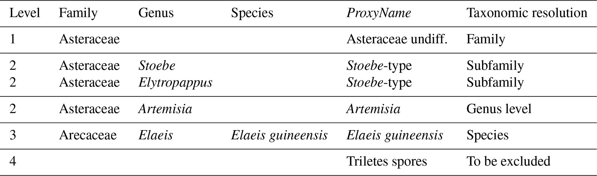
A PSE file is composed of five columns (Table 3).
The first one (Level) contains an integer that indicates the
level of taxonomic resolution of the row (1 for family, 2 for genus, 3
for species and 4 for taxa that should be excluded from the
reconstruction, e.g. “Triletes spores” in the example case
study). The fifth column, ProxyName, contains the name of the
taxon. All the taxa recorded in the df dataset should be listed
here, or they will be excluded from the study. Columns two to four
contain the taxonomic classification of that taxon as Family,
Genus and Species, respectively. For simplicity, a
pre-formatted version of the PSE table with the names of all
the taxa to study can be generated by crestr using the
createPSE() function that generates a spreadsheet with the
correct structure and with the Level and ProxyName columns
automatically filled in:
list_of_taxa <- colnames(df)[-1]
createPSE(list_of_taxa)
The species–taxon association is performed in sequential steps by the
crest.get_modern_data() function (see Sect. 5.2). First, crestr classifies the
taxa with the lowest taxonomical resolution (i.e. when
Level is equal to one) and then increases the resolution
Level by Level. In the example in Table 3,
different taxonomic resolution levels are provided for different plant
species belonging to the highly diverse Asteraceae family (the daisy
family). To distribute all the Asteraceae species observed across the
study area to their appropriate taxon, all the species are first
classified as “Asteraceae undiff.” (first row, Level = 1). In
subsequent steps, the classification of some of these Asteraceae species
is refined when reaching the better-resolved sub-groups
(Stoebe-type and Artemisia at Level = 2). At the
end of the process, the “Asteraceae undiff.” group only contains
Asteraceae species that grow in the study area but are not part of the
genera Stoebe, Elytropappus or Artemisia. The
latter are categorised separately as Stoebe-type or
Artemisia.
Additional taxa can also be added to the PSE file to exclude
species known not to be part of a group, even if the pollen grains
corresponding to these species have not been observed. For instance,
this “trick” could have been used to simplify the climate response of
the “Asteraceae undiff.” group by excluding more species from it. This
categorisation process can be time-consuming, as all the taxa must be
classified in a unique PSE table. This process will often
require a few iterations to be optimised. The results of the different
assignments are stored in the crestObj returned by the
crest.get_modern_data() function and can be evaluated by
checking rcnstrctn$misc$taxa_notes.
4.3.3 The alternative modern calibration dataset (distributions)
Users that prefer fitting proxy–climate responses from their own
calibration data instead of the proposed gbif4crest dataset
should prepare a distributions dataset following the specific
structure presented in Table 4. The first two
columns should contain species names (or any unique identifiers) and the
corresponding proxy name. If more than one species correspond to one
taxon, the PDFs will be fitted in two steps, as explained in Sect. 2. The following two columns contain the
coordinates of the species occurrence data. Finally, the last columns
contain the climate values to be reconstructed. An optional column
called weight can be added to distributions in the
fifth position (i.e. between the coordinates and the climate
variables) if one wants to weigh the different observations. For
example, the (relative) abundance of taxa observed from modern proxy
assemblages can be used when fitting the PDFs to give more importance to
the observations where that abundance is highest. This could also be
used if accurate abundance data were available instead of presence-only
data. The weights take a value between 0 and 100.
Table 4Template for the distributions data frame. The weights column, here indicated with an asterisk, is optional and can be omitted or its values all set to 1 to assign the same weight to each observation. The number of rows of the table should correspond to the number of unique occurrences available. The dots indicate that many more rows, and possibly columns, are expected in a real distributions table.

4.3.4 The climate_space data frame
This data frame is only necessary if the users use a personal
calibration dataset (distributions) instead of the
gbif4crest dataset. This data frame enables (1) using the climate
space weighting option (Sect. 2.2) and (2)
including plots of modern climate in the different diagnostic tools. Its
structure is straightforward, with the first two columns containing
longitudes and latitudes and the subsequent columns the climate
variables to reconstruct. The spatial resolution and the ordering of the
climate variables should be identical to the distributions
table (Table 4). However, the arrangement of the
rows is not important. Including a climate_space dataset is
recommended, even if it is not mandatory.
4.3.5 The selectedTaxa data frame
The last data frame that may be used to inform the reconstruction is a
data frame of ones and zeros called selectedTaxa. This data
frame has as many rows and columns as there are taxa and climate
variables, respectively. Each entry, which should be either 1 or 0,
indicates if the taxon should be used to reconstruct the climate
variable (value =1) or not (value =0). If a selectedTaxa data
frame is not provided, a default data frame with all entries set to 1 is
added to the crestObj at initialisation. Users can then modify
this information at any point using the includeTaxa() and
excludeTaxa() built-in functions. The
crest.get_modern_data() function also modifies this data
frame by setting the value to −1 when the PSE classification
failed for a taxon or when the amount of data in the study area is
insufficient to fit a reliable PDF (see the parameter description in
Sect. 5.2).
4.4 Package dependencies
The crestr package is built in R (R Core Team, 2020) using the
devtools package (Wickham et al., 2020). crestr depends
on numerous packages: clipr (Lincoln, 2020),
DBI (R Special Interest Group on Databases (R-SIG-DB) et al., 2021), openxlsx (Schauberger and Walker, 2020),
pals (Wright, 2021), plot3D (Soetaert, 2021),
plyr (Wickham, 2011), raster (Hijmans, 2021),
rgdal (Bivand et al., 2021), rgeos (Bivand and Rundel, 2020),
RPostgres (Wickham et al., 2021), scales
(Wickham and Seidel, 2020), sp (Pebesma and Bivand, 2005; Bivand et al., 2013),
stringr (Wickham, 2019) and viridis
(Garnier et al., 2021). The dedicated documentation, tutorials and
application examples found at https://mchevalier2.github.io/crestr (last access: February 2022) were
generated and formatted by the package pkgdown
(Wickham and Hesselberth, 2020).
5.1 Example application: pollen-based mean annual temperature reconstructions from marine core MD96-2048
To illustrate the different ways of using crestr and its graphical diagnostic tools, I use pollen data recently analysed with the original CREST software to reconstruct mean annual temperature (MAT) from marine core MD96-2048. The core was retrieved off the coast of South Africa and Mozambique near the mouth of the Limpopo River. The terrestrial sediments are expected to come from the entire catchment of the Limpopo River and the smaller local river catchments near the coast (Dupont et al., 2019, 2011; Castañeda et al., 2016). The MAT reconstruction is based on 181 fossil pollen samples and the percentages of more than 150 terrestrial pollen taxa and covers the last 790 000 years.
As the catchment of these marine sediments is large, an extensive calibration dataset covering all vegetation zones from tropical Africa to the temperate southwestern tip of South Africa was designed to prevent any artificial reduction in the possible range of variability of the reconstruction. The glacial–interglacial trends and amplitude of the MAT reconstructions were validated by comparing them with regional temperature records and other global indicators of glacial–interglacial temperature variability (e.g. Antarctic temperature or global sea-level curves, see Chevalier et al., 2021a, for more details). Here, I reproduce this reconstruction using the original parameterisation of the CREST algorithm obtained from the original CREST point-and-click interface to showcase how it can easily be replicated in a few lines of code with the crestr package. Due to the update of the climate data of the calibration dataset described in Sect. 3, marginal differences in the order of tenths of degrees Celsius can, however, be observed between the original publication and this reproduction. All the necessary datasets and R code are available in the Supplement.
5.2 Formatting the calibration data in a crestObj
As the gbif4crest dataset was used to fit the PDFs, the function
called crest.get_modern_data() was used to extract the
calibration data:
rcnstrctn <- crest.get_modern_data(
  df = MD96_2048,
  pse = PSE,
  selectedTaxa = selectedTaxa,
  taxaType = 1,
  climate = c('bio1'),
  xmn = NA, xmx = NA,
  ymn = -35, ymx = NA,
  continents = 'Africa',
  countries = c('South Africa', 'Kenya',
    'Lesotho', 'eSwatini', 'Botswana',
    'Mozambique', 'Zimbabwe', 'Zambia',
    'Malawi', 'Tanzania', 'Namibia',
    'Uganda', 'Rwanda', 'Burundi'),
  realms = NA,
  biomes = NA,
  ecoregions = NA,
  minGridCells = 20,
  site_info = c(34.0167, -26.1667),
  site_name = 'MD96-2048',
  dbname = "gbif4crest_02",
  verbose = TRUE)
All the parameters of the function were defined by the characteristics
of the proxy (pollen), the climate to reconstruct (MAT/bio1) and the
definition of the study area (eastern and southern Africa). The three input
files (i.e. df, PSE and selectedTaxa;
see Sect. 4.3) required to realise this
reconstruction are reproduced from the published dataset
(Chevalier et al., 2020a) and are available in the Supplement.
The following points describe the different parameters of the
crest.get_modern_data() function and how they relate to the
data extraction and modelling.
-
The parameter
taxaTypeis used to choose the type of proxy used and takes a value between 1 to 6 for plants (i.e. pollen and plant macro remains), beetles, chironomids, foraminifers, diatoms and rodents, respectively. -
The name(s) or code(s) of the
climatevariables to study should be provided here (see Tables 1 and 2 or use the functionaccClimateVariables()for a list of accepted names). Here, “bio1” means mean annual temperature. More variables can be added if necessary (e.g.c('bio1', 'ai')). However, serial reconstructions should be avoided, even if many variables are provided with this package. Careful interpretations of the fossil data should be made before selecting variables. -
Geographical parameters can be provided to tailor the gbif4crest dataset to the study area and data. These can include minimum and maximum longitude and latitude (
xmn,xmx,ymn,ymx), continent, ocean or country names (seeaccCountryNames()andaccBasinNames()for a list of accepted names), and also some ecological classifiers, such as realms, biomes or ecoregions (seeaccRealmNames()for a list of official names). Only the occurrences that respect all the specified constraints will be returned. -
To estimate reliable species PDFs, it is recommended to use at least 20 distinct occurrences for each species, even if different values can be specified with the
minGridCellparameter, depending on the density of data available across the study area. -
Optional information about the site, such as a name and coordinates, can be provided and, where possible, this information will be represented on the different graphical diagnostic tools created by crestr (e.g. the location of the record is added to the maps if the coordinates are provided).
The crest.get_modern_data() function reads all the data and
parameters, extracts the data from the cloud-based gbif4crest
database, processes the distribution data and returns everything as a
structured crestObj – here called rcnstrctn and whose
structure is displayed in Fig. 5 – that will be read
and modified by all subsequent functions. Alternatively, the function
crest.set_modern_data() could be called instead of
crest.get_modern_data() to use personal calibration data
instead of the gbif4crest database. If the calibration data
needed for this study were available as a distributions and
climate_space data frames (Sect. 4.3),
similar results would be obtained with
rcnstrctn <- crest.set_modern_data(
  df = MD96_2048,
  distributions = distributions,
  climate_space = climate_space,
  selectedTaxa = selectedTaxa,
  climate = c('bio1'),
  weight = FALSE,
  minGridCells = 20,
  site_info = c(34.0167, -26.1667),
  site_name = 'MD96-2048',
  verbose = TRUE)
5.3 Estimating the climate responses (the PDFs)
The probabilistic proxy–climate responses, i.e. the PDFs, are
estimated from the presence-only data using the
crest.calibrate() function:
rcnstrctn <- crest.calibrate(
  rcnstrctn,
  shape = c('normal'),
  climateSpaceWeighting = TRUE,
  bin_width = c(2),
  npoints = 500,
  geoWeighting = TRUE,
  verbose = TRUE)
As described in Sect. 2.2, the different parameters that control the reconstruction should be carefully considered to produce reliable PDFs. These include specifying
-
the
shapeof the species PDFs, which should be either “normal” or “lognormal”, depending on the variable to reconstruct (see Sect. 2.2). -
the width of the climate bins (
bin_width) expressed in the variables' units (e.g. 2 ∘C or 50 mm) if the PDFs are corrected for an heterogeneous climate space (climateSpaceWeightingset toTRUE). Dividing the total climate space in 15–25 bins often leads to good results, but other values are possible. -
the number of intervals required to divide the studied climate range and fit the PDFs
npoints. This will ultimately define the climate resolution of the reconstructions. crestr runs faster with lower values, but this can alter the reconstructions with visible “jumps” between consecutive climate values (aliasing effect). -
set
geoWeightingtoTRUEif the species PDFs of the different composing species should be weighted according to the square root of the extent of their modern distribution (the in Eq. 6).
5.4 Assessing the coherency of the climate space
In every study involving estimating relationships between biological entities and environmental parameters, the first step is to ensure that the defined study area and associated calibration dataset are coherent. This includes ensuring that (1) all the essential taxa observed in the past are present in the study area, and their distributions are not truncated, (2) the climate values to reconstruct are likely to be covered by present-day climate values (the reconstructions are bounded by the lowest and highest values observed in the modern climate space) and (3) there is no large sampling or representativity bias (e.g. along country borders due to different sampling efforts). The “climateSpace” graphical diagnostic tool (Fig. 6) was designed for a rapid assessment of all these characteristics:
plot_climateSpace(rcnstrctn, save=TRUE,
  filename='Figure 6.png',
  as.png=TRUE, png.res=600,
  width=6.9, height=4.4,
  y0=0.4,
  add_modern=TRUE)
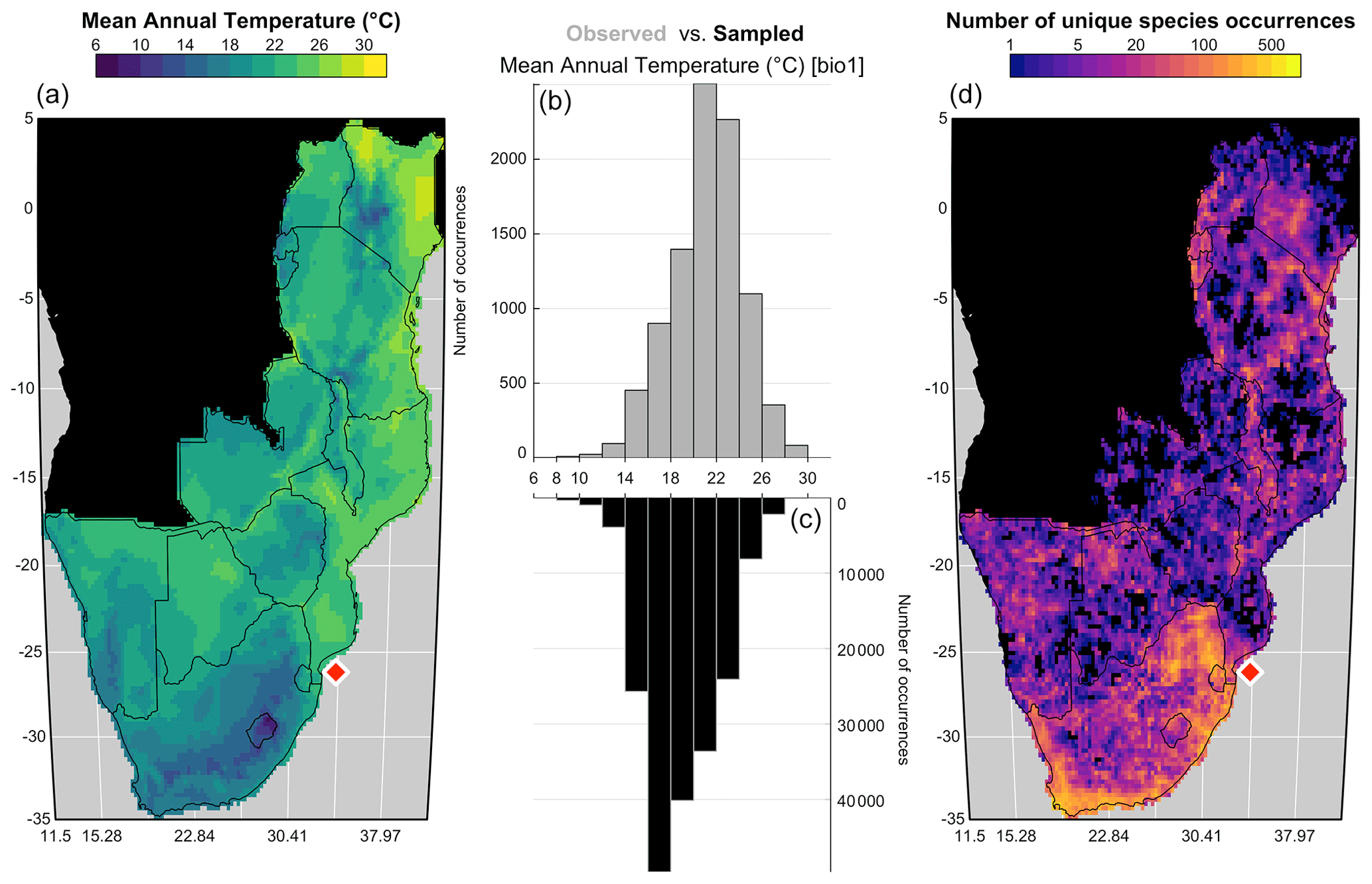
Figure 6“climateSpace” graphical diagnostic tool to evaluate the calibration dataset. The map on the right (d) represents the density of unique species occurrences in each grid cell, highlighting a certain bias towards South Africa. The lower abundance of plant data available from Angola and the Democratic Republic of Congo (data not shown) is the reason why these two countries were excluded from the study area. The map on the left (a) represents the studied climate variable (MAT) across the study area. The double histogram in the middle represents the distribution of MAT (the climate space in grey, b), while the black histogram (c) represents how the calibration data sample the climate space. Differences between the two histograms can be used to identify biases in the calibration dataset. Here, the small shift of the black histograms towards colder values (towards the left) is another way of seeing that more data are available from South Africa than other countries and reflects, in part, the regional patterns of biodiversity. If more variables had been selected in this study, additional rows would be added to the figure with a similar climate map and histograms and a scatterplot of the climate variables to highlight potential local or regional modern correlations.
Ideally, the climate values sampled by the calibration data should be as homogeneous as possible to ensure proper representation of all the possible climate values, even if the extreme climate values will always be under-represented compared to the median ones. However, deviations from a theoretical equivalence between the observed climate distribution and the climate values sampled by the calibration data are not necessarily a bad characteristic. In our case study, the variability of the sampling density represents actual patterns in regional species diversity with the presence of several biodiversity hotspots across the mountainous regions of eastern and southern Africa (Myers et al., 2000). This higher diversity in the colder areas explains why the black histogram (i.e. the climate values associated with occurrence data) in Fig. 6 is skewed towards the left compared to the grey histogram (i.e. the distribution of the climate space in the study area). All these elements should be checked and accounted for while designing the final calibration dataset.
The “climateSpace” diagnostic figure is also practical for identifying
potential local or global correlations between different climate
variables and assessing the risk of confounding variables (i.e.
variables that are correlated with important variables but do not
directly impact the studied proxies; Juggins, 2013; Chevalier et al., 2020b). Any change to the parameters related to
the definition of the climate space (e.g. definition of the study
area, climate variables to reconstruct) will require re-running
crest.get_modern_data() or crest.set_modern_data()
with updated parameters and/or data.
5.5 Assessing the coherency of the climate responses
With the study area and climate space defined, the next step is to search for taxa that show specific relationships with climate. While all species eventually respond to all climate variables, they can be more sensitive to one over another within a given region. The low taxonomic resolution of some fossil proxies, such as pollen data, can also mask strong species–climate relationships (Chevalier et al., 2021b). Looking at each individual climate response(s) and assessing their significance within the boundary conditions of the study is thus critical. The “taxaCharacteristics” diagnostic plot (Fig. 7) was designed for this task:
plot_taxaCharacteristics(rcnstrctn,
  taxanames='Ericaceae', save = TRUE,
  filename = 'Figure 7.png',
  as.png=TRUE, png.res=600,
  width=6.9, height=8.13,
  add_modern=TRUE)
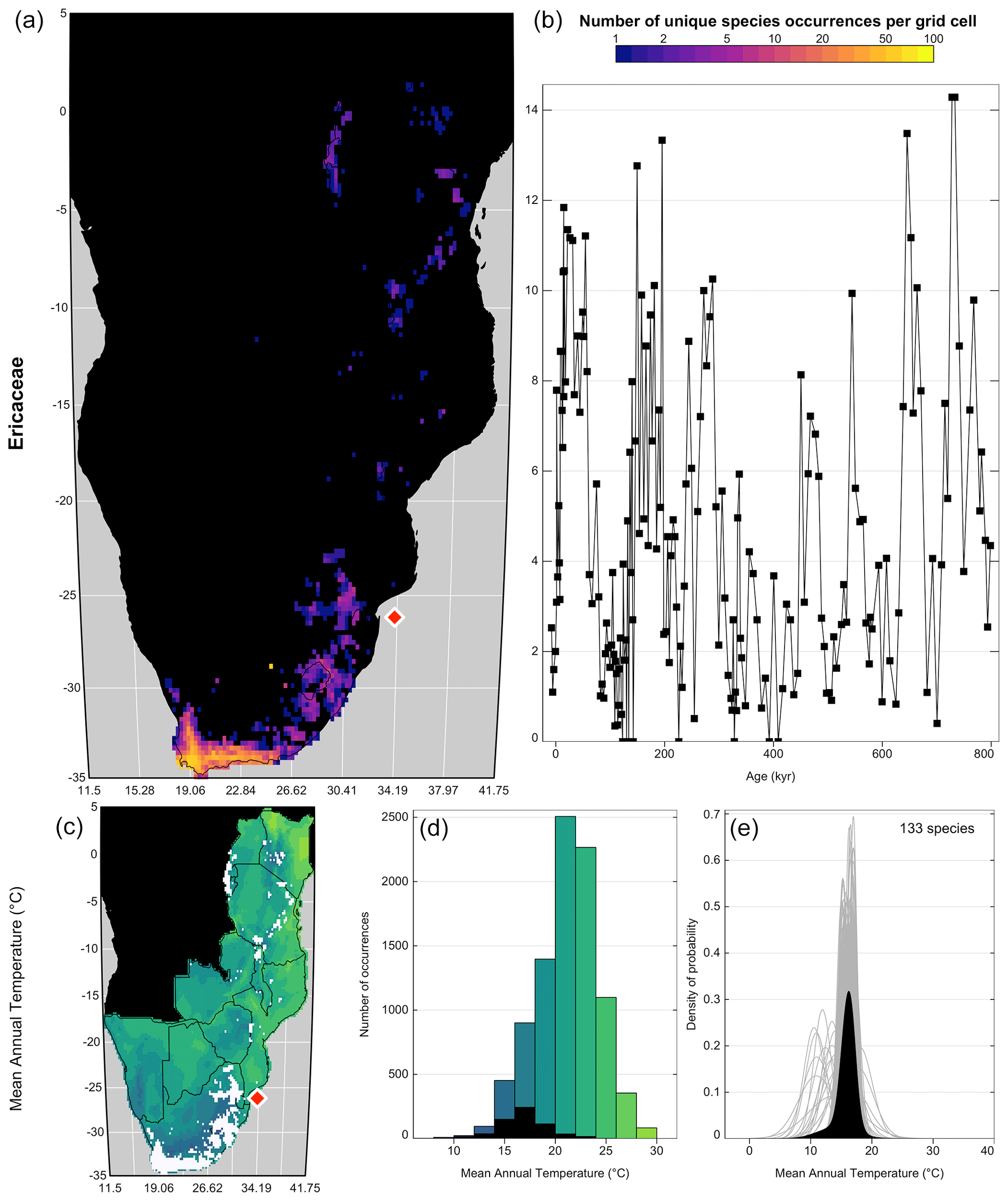
Figure 7“taxaCharacteristics” graphical diagnostic tool to assess the sensitivity of taxa to climate. In the top row (a, b), the map (a) represents the density of unique species occurrences per grid cell derived from the modern calibration dataset, and the time series (b) represents the variability of the taxon against time or depth. The bottom row (c–e) is specific to each selected variable (only one row in this case). The map (c) represents the geographical distribution of the taxon (in white) against the climate background. The histogram (d) represents the climate space (in colour) and how this climate is sampled by the taxon (in black). Finally, the right plot (e) represents the climate response of the taxon (in black) and the response of all the composing species (in grey). Overall, this figure highlights that despite its high diversity, Ericaceae is primarily associated with the colder environments of the study area and its presence increases during glacial periods. The red diamond indicates the location of the studied record.
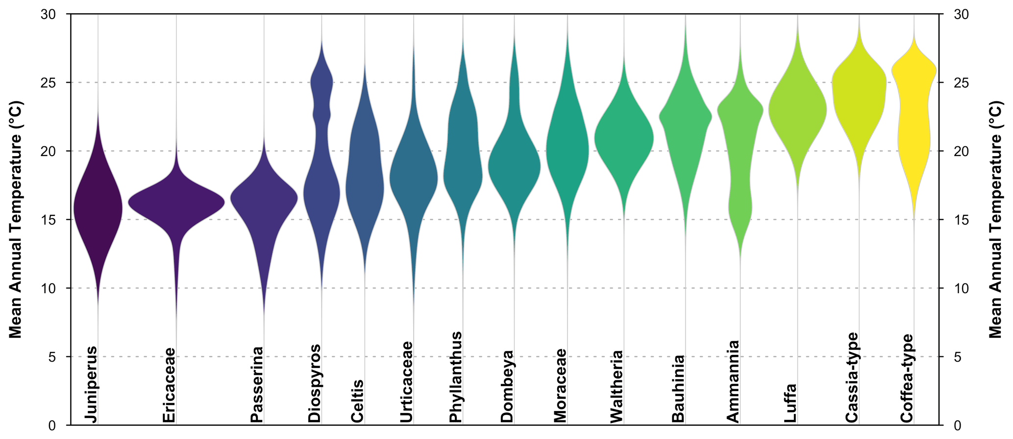
Figure 8“violinPDFs” graphical diagnostic tool to represent the PDFs of various taxa (here a random selection of 15 taxa). The taxa are sorted and colour-coded by their temperature optima (i.e. the temperature corresponding to the peak of their PDFs).
One summary plot can be generated for every taxon to assess and inter-compare their geographical distributions and climate responses. As illustrated in Fig. 7, Ericaceae is preferentially observed in the colder environments of the study area, its higher percentages occur during glacial periods, and a coherent response of all its composing species can be observed despite a high diversity (141 species with at least 20 unique occurrences across the study area). All these elements indicate that Ericaceae can be considered a cold environment indicator in eastern and southern Africa. Sensitivities to other variables can also be expected but are not considered in this study. Similar sensitivity inferences can be made to define a list of temperature-sensitive taxa to reconstruct MAT (Chevalier and Chase, 2015; Chevalier et al., 2021a) or support qualitative interpretations of palaeoecological datasets (Chevalier et al., 2021b; Quick et al., 2021). A complementary diagnostic plot to assess climate sensitivities is the “violinPDFs” (Fig. 8):
tax <- sample(rcnstrctn$input$taxa.name,
              15, replace=FALSE)

plot_violinPDFs(rcnstrctn,
  taxanames = tax,
  save = TRUE,
  filename = 'Figure 8.png',
  as.png=TRUE, png.res=600,
  width = 6.9, height = 3,
  ylim=c(0,30))
The violin plot represents the PDFs of a selection of taxa on the same plot, which helps compare the shape and spread of the different responses. All the violins have the same area (all the probabilities sum to 1), and the taxa are ranked by increasing values of their temperature optima (i.e. the temperature corresponding to the peak of the PDF). However, due to the possible multimodality of the PDFs and differences in tolerance ranges, this ranking does not mean that a taxon on the left always represents colder conditions than a taxon on the right. This is illustrated in many ways in Fig. 8 with, for example, Cassia-type that is estimated to experience warmer conditions than Coffea-type ∼61 % of the time (based on 100 000 random draws from their PDFs) despite having a “colder” climate optimum, or with Diospyros that can tolerate much warmer conditions than most taxa with warmer optima. This type of representation can be beneficial to make more informed interpretations of ecological changes from pollen diagrams (Chevalier et al., 2021b; Quick et al., 2021).
5.6 Reconstructing climate
Along with the df data frame provided to the
crest.get_modern_data() or crest.set_modern_data()
functions, a set of reconstruction parameters have to be chosen to
combine PDFs and estimate climate parameters. The selectedTaxa
data frame stored in the crestObj (see Fig. 5)
defines the taxa that will be used to reconstruct each climate variable
(by default, all taxa are included if sufficient data are available to
fit a PDF). This selection can be modified by using the
includeTaxa() and excludeTaxa() functions. For
instance, both Aizoaceae and Chenopodiaceae/Amaranthaceae were excluded
from the reconstruction because these taxa are not primarily sensitive
to temperature in southern Africa. This can be simply done as follows:
rcnstrctn <- excludeTaxa(rcnstrctn,
  taxa=c('Aizoaceae',
     'Chenopodiaceae/Amaranthaceae'),
  climate=c('bio1'))
Climate reconstructions are then performed with the
crest.reconstruct() function:
rcnstrctn <- crest.reconstruct(
  rcnstrctn,
  presenceThreshold = 0,
  taxWeight = "normalisation",
  verbose = TRUE)
A minimum “presence threshold” below which the taxa will always be
considered absent can be provided to reduce the noise of the fossil
dataset (e.g. pollen percentages lower than 1 % or 2 % are commonly
excluded from reconstructions, Chevalier et al., 2020b). When
presenceThreshold is set to zero, as is the case here, all the
strictly positive pollen percentages are considered as actual presences
and used accordingly to reconstruct MAT. To weigh the taxa as described
in Eq. (7), four options are available in crestr:
-
The data can be converted to presence/absence with all the values above and below
presenceThresholdbeing changed to ones and zeros, respectively. This option is recommended for data such as macrofossils for which relative abundances cannot be reliably estimated. -
The data can be converted to percentages to weigh the taxa according to their relative abundance. This option is recommended for data where reliable proportions can be estimated.
-
The data can be normalised following the method proposed by Chevalier et al. (2014) and described here by Eq. (8). This option is recommended for palaeoecological proxies where the observed percentages are not proportional to their abundance in the environment, such as pollen data.
-
The data can be directly weighted by the values provided in
df, which implies that users can define their own specific weighting strategy (e.g. using the square-root transformation of the pollen percentages).
5.7 Analysing and understanding the reconstruction(s)
Characterising the dominant factors that define a reconstruction can be
difficult. This section presents three different graphical diagnostic
tools that provide different perspectives on the reconstructed data and
help look inside the statistical black box. First, the full
probabilistic breadth of the reconstructions can be represented by using
the standard R plot() function (Fig. 9), which
has been adapted to plot data stored in a crestObj:
plot(rcnstrctn,
  filename='Figure 9.png',
  save=TRUE,
  as.png=TRUE, png.res=600,
  width=6.9, height=3.54,
  ylim=c(14,23), uncertainties=1,
  simplify=FALSE,
  col=plot3D::gg2.col(200)[1:100],
  pt.cex=0.8, pt.lwd=1, pt.col='#2c2c2c')
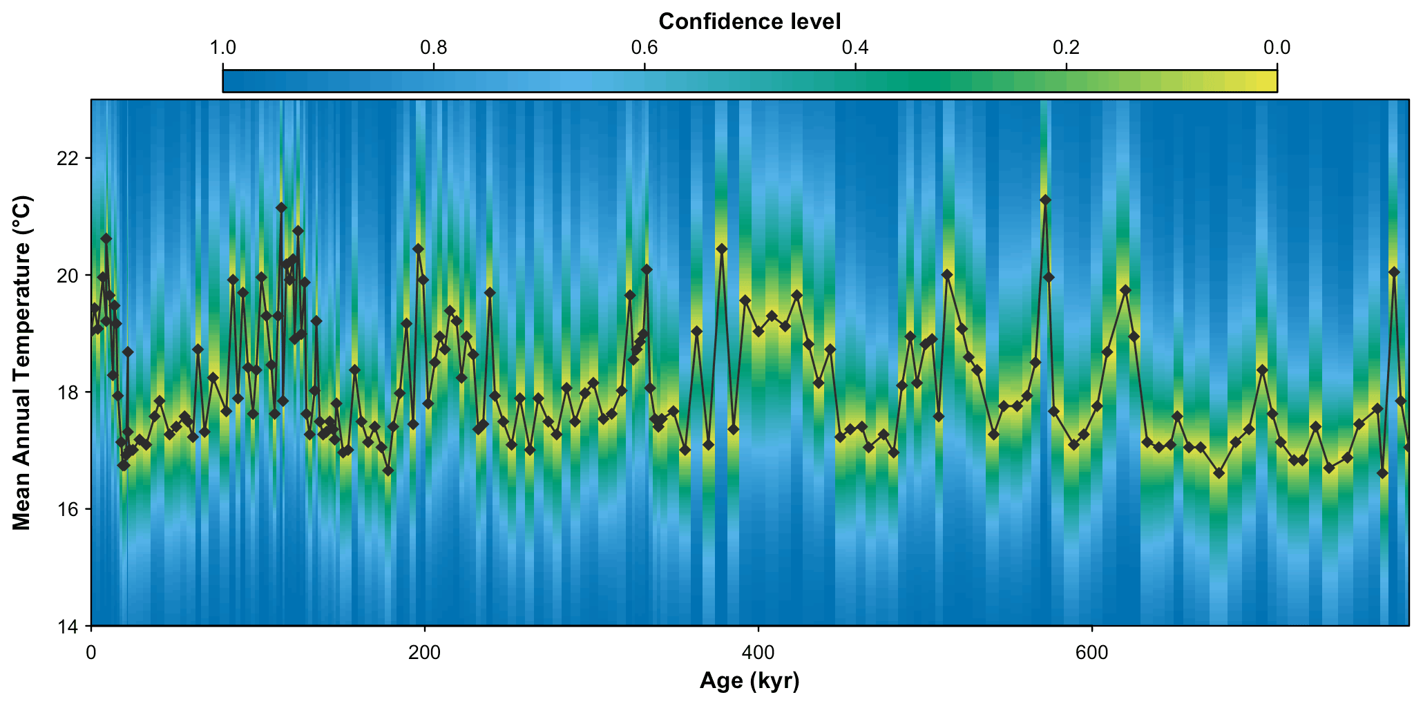
Figure 9MAT probabilistic reconstructions for marine core MD96-2048. The yellow–green–blue colour gradient represents the uncertainties associated with each sample. This reconstruction is identical to the reconstruction presented in Chevalier et al. (2021), and the reader is referred to this publication for an in-depth validation and discussion of these results.

Figure 10“combinedPDFs” graphical diagnostic tool that shows the combination of the PDFs (in colour) of all the taxa recorded in the sample dated at 64 kyr. The thickness of the lines is related to the weight of the taxa in the sample (absolute value indicated next to each taxon name). The black curve represents the MAT reconstruction, from which a “best” climate estimate can be estimated from the maximum of the curve (grey dashed line) and uncertainties derived by calculating the area under the curve.
While the probabilistic representation of the data should be preferred
because it represents all the information available, a simpler version
of this plot with the climate optima and more common uncertainty ranges
expressed as colour bands can be obtained by specifying
simplify=TRUE (not shown).
The plot_combinedPDFs() function can then be used to identify
the taxa that are driving the reconstruction by focusing on the sample
level:
plot_combinedPDFs(rcnstrctn,
    samples=3, only.present=TRUE,
    only.selected=TRUE, save = TRUE,
    filename = 'Figure 10.png',
    as.png=TRUE, png.res=600,
    width=6.9, height=3,
    xlim=c(7.5,32.5))
In this plot (Fig. 10), the PDFs of all the taxa
present in the sample and selected to reconstruct the climate variable
are represented along with the reconstruction. This type of plot can
help identify if a particular PDF is at odds with the general
assemblage, which usually indicates the possible presence of a
confounding factor. It is also helpful to visualise the full spread of
the uncertainties and, by extension, highlight that reconstructions can
be multimodal. While it is not the case in the example here,
multimodality can be the underlying cause of apparent noise in the
reconstructions with minor changes in the taxa composition or
percentages forcing the system to oscillate between two maxima and thus
“appear” noisy. This effect could also be seen from the reconstruction
plot where the full uncertainties would be represented
(simplify=FALSE).
Finally, a standard post-processing analysis of CREST reconstructions is
a form of leave-one-out (LOO) analysis that is done with the
loo() function:
rcnstrctn <- loo(rcnstrctn,
  verbose = TRUE)
In the CREST context, a LOO analysis consists of repeatedly “unselecting” one taxon at a time, running the reconstruction without that taxon and measuring the associated reconstruction anomalies. In our example, a positive anomaly means that the reconstruction without the taxon is warmer and, by extension, that the taxon is a cold indicator relative to a specific assemblage. A detailed analysis of the results can contribute to a deeper understanding of which taxa are the most important in driving the reconstructed climate signal. Taxa that exhibit large LOO values indicate a strong influence on the reconstruction. However, it does not necessarily mean that they are strong climate indicators. Large LOO values can arise when the PDFs are biased by unaccounted factors and are, as a result, at odds with the rest of the PDFs. Such factors can, for instance, include an incomplete estimate of the climate responses, which induces a bias or shift of the climate preferences, or a sensitivity of the taxon to other climatic (e.g. aridity instead of temperature) or non-climatic (e.g. edaphic conditions) factors. It is usually preferable to exclude such taxa from the reconstruction (e.g. Chenopodiaceae and Aizoaceae in our example).
The LOO analysis is a powerful tool to understand the taxa that primarily drive the reconstruction, and the LOO results can be represented as a typical stratigraphic diagram, where each row illustrates the effect of removing a taxon from the reconstruction (Fig. 11):
tax <- rcnstrctn$inputs$taxa.name[6:25]
plot_loo(rcnstrctn,
    taxanames=tax,
    xlim=c(0, 340), save = TRUE,
    filename = 'Figure 11.png',
    as.png=TRUE, png.res=600,
    width=3.5, height=8,
    bar_width=3, col_neg='coral3',
    col_pos='darkcyan')
For example, the expected cold effect of including Ericaceae on the MAT reconstructions from the MD96-2048 pollen record is immediately visible in Fig. 11. Similarly, the effect of removing either Ericaceae or Caryophyllaceae undiff. from the sample dated at 64 kyr (represented in Fig. 10) is quite strong with a warming of the reconstruction of 1.19 and 0.44 ∘C, respectively. This type of plot can thus be used for both global and sample-specific inferences about the drivers of the reconstruction. Depending on the vegetation composition, some taxa can even sometimes be categorised as cold indicators when the assemblage represents warm conditions or warm indicators when the assemblage represents cold conditions (e.g. Hypoestes/Dicliptera-type in Fig. 11).
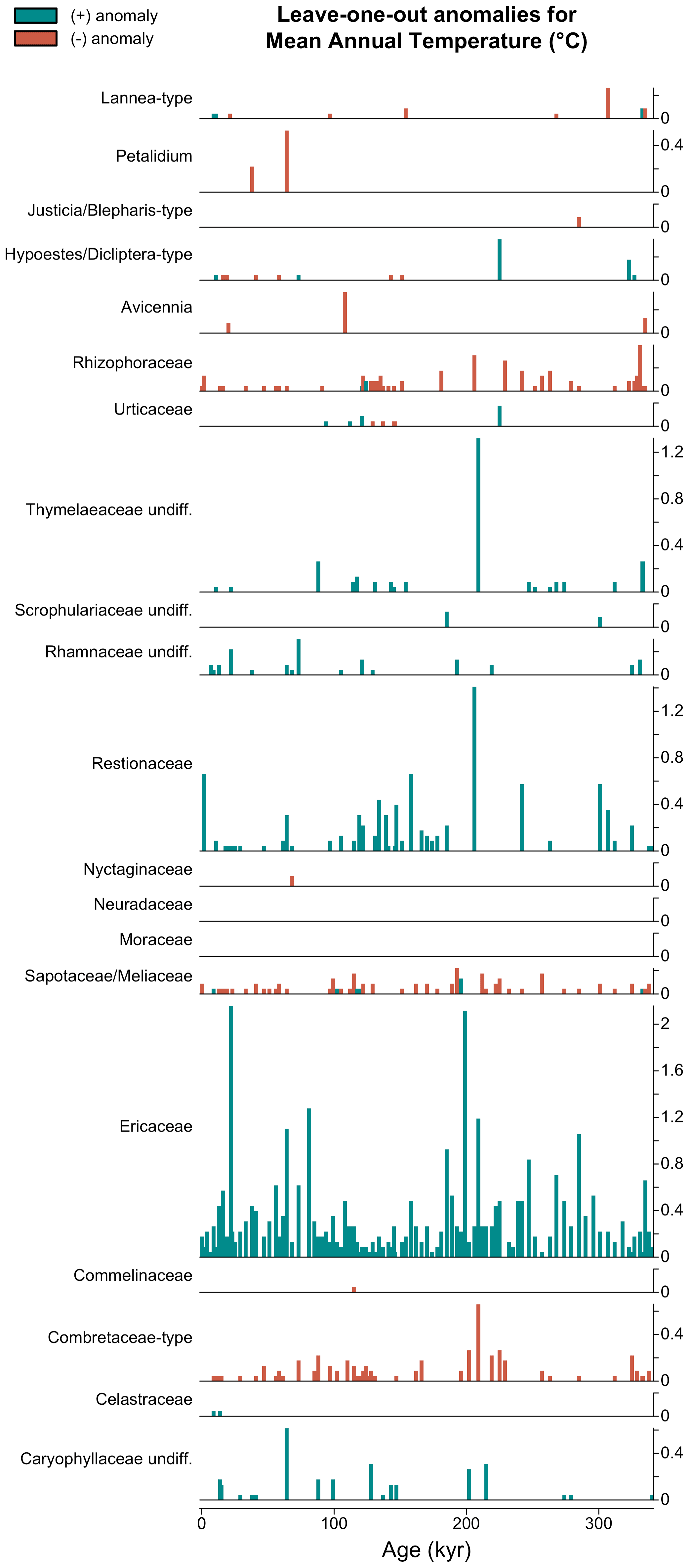
Figure 11Leave-one-out (LOO) graphical diagnostic tool to illustrate the influence of different taxa on the reconstructions. Here, the results are only shown for a subset of the taxa observed in marine core MD96-2048 (only 20 out of the 171 available taxa are represented). The height of each bar represents the absolute effect (in ∘C) of removing the taxon from the reconstruction, and the sign of this effect (increase or decrease of the reconstructed temperature) is colour-coded. Here, blue (cf. Ericaceae) and red (cf. Combretaceae-type) bars indicate that the taxon is a cold and warm indicator, respectively, in the sample.
5.8 A wrapper function
To simplify the use of the package, the three stages of the
reconstruction process – data acquisition
(crest.get_modern_data() or
crest.set_modern_data() if the gbif4crest dataset is
not used), calibration (crest.calibrate()) and reconstruction
(crest.reconstruct()) – can be called in one line of code
using the wrapper function crest(). This function takes the
same parameters described in this “step-by-step” guide with the same
default values and may be more practical when reconstructing several
records in one run.
5.9 Exporting the reconstructions
All the data stored in the crestObj can be easily exported from
the R environment as spreadsheets and RData files using either
export_pdfs() to save the climate responses of the studied
taxa or export() to save the reconstructions and many
associated data in a publishable format. The latter also saves the
crestObj as an RData file for easy reloading and sharing of the
data:
export(rcnstrctn,
  loc='path/to/folder',
  fullUncertainties = TRUE,
  loo = TRUE,
  weights = TRUE,
  pdfs = TRUE)
5.10 Citing building elements
Finally, all the reconstructions derived from crestr are built on
numerous independent research efforts, including data compilations,
modelling projects, statistical developments and software engineering.
To support the long-term growth and visibility of all these building
elements, it is crucial always to acknowledge them, even if their
processing is invisible to the users. The list of references that must
be cited for each use of crestr is automatically included in the
summary tab of the spreadsheet generated by the export()
function. In addition, the citation information can also be directly
obtained from R:
cite_crest(rcnstrctn)
The function looks at the type of data used in the analysis (e.g. the subset of the GBIF data were used and the climate variables) and returns a corresponding list of references. For example, a simple way of crediting all the contributors for the MAT reconstruction from marine core MD96-2048 presented here could be the following: To create this MAT reconstruction from the pollen record from marine core MD96-2048 (Dupont et al., 2019), we employed the CREST method (Chevalier et al., 2014; Chevalier, 2019). The PDFs were estimated by combining the MAT field of Fick and Hijmans (2017) and plant occurrence data from GBIF (GBIF, 2020m, k, g). The numerical analyses were realised with the crestr R package v1.0.1 (this reference).
CREST is a probabilistic framework designed to model proxy–climate relationships from modern presence observations and to use these relationships to reconstruct past climate (Chevalier et al., 2014). The method's mathematics and assumptions enable an easy application everywhere, even in data-sparse regions. While developments to complexify the method are possible, the current version of the algorithm has proven to be reliable at producing high-quality reconstructions. The first version of the crestr R package is thus dedicated to implementing the original version of the algorithm. It also replaces the original point-and-click CREST software, which was challenging to maintain over time. A critical novelty of crestr is the inclusion of the CREST algorithm in a programmatic environment. The benefits of this transition are significant and include improved scriptability (i.e. the possibility of analysing many records automatically and sequentially), reproducibility (i.e. the capacity to reproduce an analysis) and better inter-operability (i.e. R packages are compatible with all computer systems). However, maintaining the highest level of accessibility remained at the core of the development process and is illustrated in the final product by the small number of functions necessary to run a complete analysis and the suite of detailed graphical diagnostic figures. In line with the objectives of the original software, the crestr package is aimed at all researchers interested in using CREST to reconstruct climate from palaeoecological datasets, including those with limited coding expertise.
In addition, its broad applicability will allow taking advantage of the recent growth of curated, open-access fossil datasets that offer unprecedented opportunities to reconstruct climate from a wide range of proxies, particularly in regions where quantified climate reconstructions are urgently needed. This package will thus also contribute to the current transition from single-site to multi-site studies, which is necessary to better understand past climate dynamics. However, it is essential to remember that running such techniques on several datasets should always be done carefully, as many factors can impact the reconstruction process. In practice, calibration datasets, variable selection and reconstructions should be assessed, ideally against independent evidence when they are available, even if there is no single way to validate a reconstruction (but see Chevalier et al., 2020b, for some discussions on the generic principles).
Over time, the crestr package will be enriched with new functionalities to facilitate reconstruction validation. The online documentation will also be updated with diverse examples and tutorials based on real applications and assessments (https://mchevalier2.github.io/crestr/, last access: February 2022). Future package updates will include Bayesian modules and propose more complex strategies to estimate proxy–climate relationships from data-dense regions. Finally, bug reports, feedback, and suggestions for newer functionalities and graphical diagnostic tools are encouraged and can be transmitted to the author directly or through GitHub's bug report portal (https://github.com/mchevalier2/crestr/issues, last access: February 2022).
The crestr package is currently accessible from CRAN (https://CRAN.R-project.org/package=crestr, last access: 13 April 2022, Chevalier, 2022b). The version used in this paper (v1.0.1) is available on Zenodo (https://doi.org/10.5281/zenodo.6458405, Chevalier, 2022a) and future development versions will be available on GitHub (https://github.com/mchevalier2/crestr, last access: February 2022), where I also welcome feedback and strongly encourage contributions via the issue tracker (https://github.com/mchevalier2/crestr/issues, last access: 13 April 2022). The source data used for the example application (pollen record from marine core MD96-2048 and associated temperature reconstructions) can be accessed from https://doi.org/10.1594/PANGAEA.915923 (Chevalier et al., 2020a). NOAA High-Resolution SST data were provided by the NOAA/OAR/ESRL PSL, Boulder, Colorado, USA, from their website at https://psl.noaa.gov/data/gridded/data.noaa.oisst.v2.highres.html (last access: September 2021, Reynolds et al., 2007).
The supplement related to this article is available online at: https://doi.org/10.5194/cp-18-821-2022-supplement.
The author has declared that there are no competing interests.
Publisher's note: Copernicus Publications remains neutral with regard to jurisdictional claims in published maps and institutional affiliations.
I thank Brian Chase, Yoshi Maezumi, Lynne Quick, Kale Sniderman and, last but not least, Mine Altinli for their invaluable feedback on early versions of the package and manuscript. And finally, I would also like to address a special thanks to the rticles contributors for their Climate of the Past R Markdown template!
This research has been supported by the Swiss National Science
Foundation (grant no. CRSK-2_195875), with additional support from the
University of Lausanne. Manuel Chevalier is also supported by the German Federal
Ministry of Education and Research (BMBF) as a Research for
Sustainability initiative (FONA; https://www.fona.de/en, last access: 15 December 2021) through the PalMod Phase II project (grant no. FKZ:
01LP1926D).
This open-access publication was funded by the University of Bonn.
This paper was edited by Denis-Didier Rousseau and reviewed by two anonymous referees.
Amante, C. and Eakins, B. W.: Etopo1 1 Arc-Minute Global Relief Model: Procedures, Data Sources and Analysis, NOAA Technical Memorandum NESDIS NGDC-24, National Geophysical Data Center, NOAA [data set], https://doi.org/10.7289/V5C8276M, 2009. a
Birks, H. J. B., Heiri, O., Seppä, H., and Bjune, A. E.: Strengths and weaknesses of quantitative climate reconstructions based on Late-Quaternary biological proxies, The Open Ecology Journal, 3, 68–110, https://doi.org/10.2174/1874213001003020068, 2010. a
Bivand, R. and Rundel, C.: rgeos: Interface to Geometry Engine – Open Source (“GEOS”), r package version 0.5-5, https://CRAN.R-project.org/package=rgeos (last access: February 2022), 2020. a
Bivand, R., Keitt, T., and Rowlingson, B.: rgdal: Bindings for the “Geospatial” Data Abstraction Library, r package version 1.5-23, https://CRAN.R-project.org/package=rgdal (last access: February 2022), 2021. a
Bivand, R. S., Pebesma, E., and Gomez-Rubio, V.: Applied spatial data analysis with R, 2nd edn., Springer, NY, ISBN: 978-1-4614-7617-7, https://asdar-book.org/ (last access: February 2022), 2013. a
Bray, P. J., Blockley, S. P., Coope, G. R., Dadswell, L. F., Elias, S. A., Lowe, J. J., and Pollard, A. M.: Refining mutual climatic range (MCR) quantitative estimates of palaeotemperature using ubiquity analysis, Quaternary Sci. Rev., 25, 1865–1876, https://doi.org/10.1016/j.quascirev.2006.01.023, 2006. a
Castañeda, I. S., Caley, T., Dupont, L. M., Kim, J.-H., Malaizé, B., and Schouten, S.: Middle to Late Pleistocene vegetation and climate change in subtropical southern East Africa, Earth Planet. Sc. Lett., 450, 306–316, https://doi.org/10.1016/j.epsl.2016.06.049, 2016. a
Chase, B. M., Boom, A., Carr, A. S., Carré, M., Chevalier, M., Meadows, M. E., Pedro, J. B., Stager, J. C., and Reimer, P. J.: Evolving southwest African response to abrupt deglacial North Atlantic climate change events, Quaternary Sci. Rev., 121, 132–136, https://doi.org/10.1016/j.quascirev.2015.05.023, 2015a. a
Chase, B. M., Lim, S., Chevalier, M., Boom, A., Carr, A. S., Meadows, M. E., and Reimer, P. J.: Influence of tropical easterlies in the southwestern Cape of Africa during the Holocene, Quaternary Sci. Rev., 107, 138–148, 2015b. a
Chevalier, M.: Enabling possibilities to quantify past climate from fossil assemblages at a global scale, Global Planet. Change, 175, 27–35, https://doi.org/10.1016/j.gloplacha.2019.01.016, 2019. a, b, c, d, e
Chevalier, M.: GBIF database for CREST, figshare, https://doi.org/10.6084/m9.figshare.6743207, 2020. a, b
Chevalier, M.: crestr: v1.0.1 (v1.0.1), Zenodo [code], https://doi.org/10.5281/zenodo.6458405, 2022a. a
Chevalier, M.: crestr: an R package to perform probabilistic climate reconstructions from palaeoecological datasets, R package version 1.0.1, https://CRAN.R-project.org/package=crestr (last access: 13 April 2022), 2022b. a
Chevalier, M. and Chase, B. M.: Southeast African records reveal a coherent shift from high- to low-latitude forcing mechanisms along the east African margin across last glacial–interglacial transition, Quaternary Sci. Rev., 125, 117–130, https://doi.org/10.1016/j.quascirev.2015.07.009, 2015. a, b, c, d
Chevalier, M. and Chase, B. M.: Determining the drivers of long-term aridity variability: a southern African case study, J. Quaternary Sci., 31, 143–151, https://doi.org/10.1002/jqs.2850, 2016. a
Chevalier, M., Cheddadi, R., and Chase, B. M.: CREST (Climate REconstruction SofTware): a probability density function (PDF)-based quantitative climate reconstruction method, Clim. Past, 10, 2081–2098, https://doi.org/10.5194/cp-10-2081-2014, 2014. a, b, c, d, e, f, g, h, i
Chevalier, M., Chase, B. M., Quick, L. J., Dupont, L. M., and Johnson, T. C.: Mean Annual Temperature changes reconstructions from marine core MD96-2048, PANGAEA [data set], https://doi.org/10.1594/PANGAEA.915923, 2020a. a, b
Chevalier, M., Davis, B. A. S., Heiri, O., Seppä, H., Chase, B. M., Gajewski, K., Lacourse, T., Telford, R. J., Finsinger, W., Guiot, J., Kühl, N., Maezumi, S. Y., Tipton, J. R., Carter, V. A., Brussel, T., Phelps, L. N., Dawson, A., Zanon, M., Vallé, F., Nolan, C., Mauri, A., de Vernal, A., Izumi, K., Holmström, L., Marsicek, J., Goring, S. J., Sommer, P. S., Chaput, M., and Kupriyanov, D.: Pollen-based climate reconstruction techniques for late Quaternary studies, Earth-Sci. Rev., 210, 103384, https://doi.org/10.1016/j.earscirev.2020.103384, 2020b. a, b, c, d, e, f, g, h, i
Chevalier, M., Chase, B. M., Quick, L. J., Dupont, L. M., and Johnson, T. C.: Temperature change in subtropical southeastern Africa during the past 790 000 yr, Geology, 49, 71–75, https://doi.org/10.1130/G47841.1, 2021a. a, b, c, d, e, f
Chevalier, M., Chase, B. M., Quick, L. J., and Scott, L.: An atlas of southern African pollen types and their climatic affinities, Palaeoecol. Afr., 35, 239–258, https://doi.org/10.1201/9781003162766-15, 2021b. a, b, c, d, e
Cordova, C. E., Scott, L., Chase, B. M., and Chevalier, M.: Late Pleistocene-Holocene vegetation and climate change in the Middle Kalahari, Lake Ngami, Botswana, Quaternary Sci. Rev., 171, 199–215, https://doi.org/10.1016/j.quascirev.2017.06.036, 2017. a
Costello, M. J., Tsai, P., Wong, P. S., Cheung, A. K. L., Basher, Z., and Chaudhary, C.: Marine biogeographic realms and species endemicity, Nat. Commun., 8, 1–9, https://doi.org/10.1038/s41467-017-01121-2, 2017. a
Dupont, L. M., Caley, T., Kim, J.-H., Castañeda, I., Malaizé, B., and Giraudeau, J.: Glacial-interglacial vegetation dynamics in South Eastern Africa coupled to sea surface temperature variations in the Western Indian Ocean, Clim. Past, 7, 1209–1224, https://doi.org/10.5194/cp-7-1209-2011, 2011. a
Dupont, L. M., Caley, T., and Castañeda, I. S.: Effects of atmospheric CO2 variability of the past 800 kyr on the biomes of southeast Africa, Clim. Past, 15, 1083–1097, https://doi.org/10.5194/cp-15-1083-2019, 2019. a, b
Fick, S. E. and Hijmans, R. J.: WorldClim 2: new 1 km spatial resolution climate surfaces for global land areas, Int. J. Climatol., 37, 4302–4315, https://doi.org/10.1002/joc.5086, 2017. a, b
Garcia, H. E., Weathers, K., Paver, C., Smolyar, I., Boyer, T., Locarnini, M., Zweng, M., Mishonov, A., Baranova, O., Seidov, D., and Reagan, J.: World Ocean Atlas 2018, Vol. 3: Dissolved Oxygen, Apparent Oxygen Utilization, and Dissolved Oxygen Saturation, NOAA Atlas NESDIS 83, 38 pp., https://archimer.ifremer.fr/doc/00651/76337/ (last access: September 2021), 2019a. a
Garcia, H. E., Weathers, K., Paver, C., Smolyar, I., Boyer, T., Locarnini, M., Zweng, M., Mishonov, A., Baranova, O., Seidov, D., and Reagan, J.: World Ocean Atlas 2018, Vol. 4: Dissolved Inorganic Nutrients (phosphate, nitrate and nitrate+nitrite, silicate), NOAA Atlas NESDIS 84, 35 pp., https://archimer.ifremer.fr/doc/00651/76336/ (last access: September 2021), 2019b. a
Garnier, S., Ross, N., Rudis, boB, Filipovic-Pierucci, A., Galili, T., timelyportfolio, Greenwell, B., Sievert, C., Harris, D. J., and Chen, J. J. : sjmgarnier/viridis: viridis 0.6.0, Version v0.6.0pre, Zenodo [code], https://doi.org/10.5281/zenodo.4679424, 2021. a
GBIF: GBIF: Global Biodiversity Information Facility, https://www.gbif.org (last access: August 2021), 2018. a
GBIF: Beetles occurrence data, downloaded on 24 September 2020, The Global Biodiversity Information Facility (GBIF) [data set], https://doi.org/10.15468/dl.nteruy, 2020a. a
GBIF: Chironomids occurrence data, downloaded on 24 September 2020, The Global Biodiversity Information Facility (GBIF) [data set], https://doi.org/10.15468/dl.jv3wsh, 2020b. a
GBIF: Diatoms occurrence data, downloaded on 24 September 2020, The Global Biodiversity Information Facility (GBIF) [data set], https://doi.org/10.15468/dl.vfr257, 2020c. a
GBIF: Foraminifera occurrence data, downloaded on 24 September 2020, The Global Biodiversity Information Facility (GBIF) [data set], https://doi.org/10.15468/dl.692yg6, 2020d. a
GBIF: Rodentia occurrence data, downloaded on 24 September 2020, The Global Biodiversity Information Facility (GBIF) [data set], https://doi.org/10.15468/dl.fscw6q, 2020e. a
GBIF: Cycadopsidae occurrence data, downloaded on 24 September 2020, The Global Biodiversity Information Facility (GBIF) [data set], https://doi.org/10.15468/dl.sfjzxu, 2020f. a
GBIF: Magnoliopsida occurrence data, downloaded on 24 September 2020, The Global Biodiversity Information Facility (GBIF) [data set], https://doi.org/10.15468/dl.ra49dt, 2020g. a, b
GBIF: Anthocerotopsida occurrence data, downloaded on 24 September 2020, The Global Biodiversity Information Facility (GBIF) [data set], https://doi.org/10.15468/dl.t9zenf, 2020h. a
GBIF: Gingkoopsidae occurrence data, downloaded on 24 September 2020, The Global Biodiversity Information Facility (GBIF) [data set], https://doi.org/10.15468/dl.da9wz8, 2020i. a
GBIF: Gnetopsidae occurrence data, downloaded on 24 September 2020, The Global Biodiversity Information Facility (GBIF) [data set], https://doi.org/10.15468/dl.h2kjnc, 2020j. a
GBIF: Liliopsida occurrence data, downloaded on 24 September 2020, The Global Biodiversity Information Facility (GBIF) [data set], https://doi.org/10.15468/dl.axv3yd, 2020k. a, b
GBIF: Lycopodiopsida occurrence data, downloaded on 24 September 2020, The Global Biodiversity Information Facility (GBIF) [data set], https://doi.org/10.15468/dl.ydhyhz, 2020l. a
GBIF: Pinopsidae occurrence data, downloaded on 24 September 2020, The Global Biodiversity Information Facility (GBIF) [data set], https://doi.org/10.15468/dl.x2r7pa, 2020m. a, b
GBIF: Polypodiopsida occurrence data, downloaded on 24 September 2020, The Global Biodiversity Information Facility (GBIF) [data set], https://doi.org/10.15468/dl.87tbp6, 2020n. a
GBIF: Bryophyta occurrence data, downloaded on 2 August 2021, The Global Biodiversity Information Facility (GBIF) [data set], https://doi.org/10.15468/DL.WD527G, 2021a. a
GBIF: Marchantiophyta occurrence data, downloaded on 2 August 2021, The Global Biodiversity Information Facility (GBIF) [data set], https://doi.org/10.15468/DL.M2SSE4, 2021b. a
Gibson, M. E., McCoy, J., O'Keefe, J. M. K., Nuñez Otaño, N. B., Warny, S., and Pound, M. J.: Reconstructing terrestrial paleoclimates: a comparison of the Co-existence Approach, Bayesian and probability reconstruction techniques using the UK Neogene, Paleoceanography and Paleoclimatology, 37, e2021PA004358, https://doi.org/10.1029/2021PA004358, 2022. a
Hijmans, R. J.: raster: Geographic Data Analysis and Modeling, r package version 3.4-13, https://CRAN.R-project.org/package=raster (last access: February 2022), 2021. a
Hui, Z., Zhou, X., Chevalier, M., Wei, X., Pan, Y., and Chen, Y.: Miocene East Asia summer monsoon precipitation variability and its possible driving forces, Palaeogeogr. Palaeocl., 581, 110609, https://doi.org/10.1016/j.palaeo.2021.110609, 2021. a
Hutson, W. H.: Application of transfer functions to Indian Ocean planktonic Foraminifera, Quaternary Res., 9, 87–112, https://doi.org/10.1016/0033-5894(78)90084-4, 1978. a
Juggins, S.: Quantitative reconstructions in palaeolimnology: new paradigm or sick science?, Quaternary Sci. Rev., 64, 20–32, https://doi.org/10.1016/j.quascirev.2012.12.014, 2013. a
Kühl, N., Gebhardt, C., Litt, T., and Hense, A.: Probability Density Functions as Botanical-Climatological Transfer Functions for Climate Reconstruction, Quaternary Res., 58, 381–392, https://doi.org/10.1006/qres.2002.2380, 2002. a, b
Lim, S., Chase, B. M., Chevalier, M., and Reimer, P. J.: 50 000 years of climate in the Namib Desert, Pella, South Africa, Palaeogeogr. Palaeocl., 451, 197–209, https://doi.org/10.1016/j.palaeo.2016.03.001, 2016. a
Lincoln, M.: clipr: Read and Write from the System Clipboard, r package version 0.7.1, https://CRAN.R-project.org/package=clipr (last access: February 2022), 2020. a
Locarnini, R., Mishonov, A., Baranova, O., Boyer, T., Zweng, M., Garcia, H. E., Reagan, J., Seidov, D., Weathers, K., Paver, C., and Smolyar, I.: World ocean atlas 2018, Vol. 1: Temperature, NOAA Atlas NESDIS 81, 52pp., https://archimer.ifremer.fr/doc/00651/76338/ (last access: September 2021), 2019. a
Myers, N., Mittermeier, R. A., Mittermeier, C. G., da Fonseca, G. A. B., and Kent, J.: Biodiversity hotspots for conservation priorities, Nature, 403, 853–858, https://doi.org/10.1038/35002501, 2000. a
Olson, D. M., Dinerstein, E., Wikramanayake, E. D., Burgess, N. D., Powell, G. V. N., Underwood, E. C., D'amico, J. A., Itoua, I., Strand, H. E., Morrison, J. C., Loucks, C. J., Allnutt, T. F., Ricketts, T. H., Kura, Y., Lamoreux, J. F., Wettengel, W. W., Hedao, P., and Kassem, K. R.: Terrestrial Ecoregions of the World: A New Map of Life on Earth: A new global map of terrestrial ecoregions provides an innovative tool for conserving biodiversity, BioScience, 51, 933, https://doi.org/10.1641/0006-3568(2001)051[0933:TEOTWA]2.0.CO;2, 2001. a
Overpeck, J. T., Webb III, T., and Prentice, I. C.: Quantitative interpretation of fossil pollen spectra: Dissimilarity coefficients and the method of modern analogs, Quaternary Res., 23, 87–108, https://doi.org/10.1016/0033-5894(85)90074-2, 1985. a
Pebesma, E. J. and Bivand, R. S.: Classes and methods for spatial data in R, R News, 5, 9–13, https://CRAN.R-project.org/doc/Rnews/ (last access: February 2022), 2005. a
Quick, L. J., Chase, B. M., Carr, A. S., Chevalier, M., Grobler, B. A., and Meadows, M. E.: A 25 000 year record of climate and vegetation change from the southwestern Cape coast, South Africa, Quaternary Res., 105, 1–18, https://doi.org/10.1017/qua.2021.31, 2021. a, b, c
R Core Team: R: A Language and Environment for Statistical Computing, R Foundation for Statistical Computing, Vienna, Austria, https://www.R-project.org/ (last access: February 2022), 2020. a
R Special Interest Group on Databases (R-SIG-DB), Wickham, H., and Müller, K.: DBI: R Database Interface, r package version 1.1.1, https://CRAN.R-project.org/package=DBI (last access: February 2022), 2021. a
Reynolds, R. W., Smith, T. M., Liu, C., Chelton, D. B., Casey, K. S., and Schlax, M. G.: Daily high-resolution-blended analyses for sea surface temperature, J. Climate, 20, 5473–5496, https://doi.org/10.1175/2007JCLI1824.1, 2007 (data available at: https://psl.noaa.gov/data/gridded/data.noaa.oisst.v2.highres.html, last access: September 2021). a, b
Schauberger, P. and Walker, A.: openxlsx: Read, Write and Edit xlsx Files, r package version 4.2.3, https://CRAN.R-project.org/package=openxlsx (last access: ), 2020. a
Soetaert, K.: plot3D: Plotting Multi-Dimensional Data, r package version 1.4, https://CRAN.R-project.org/package=plot3D (last access: February 2022), 2021. a
ter Braak, C. J. F. and van Dame, H.: Inferring pH from diatoms: a comparison of old and new calibration methods, Hydrobiologia, 178, 209–223, https://doi.org/10.1007/BF00006028, 1989. a
ter Braak, C. J. F. and Juggins, S.: Weighted averaging partial least squares regression (WA-PLS): an improved method for reconstructing environmental variables from species assemblages, Hydrobiologia, 269, 485–502, https://doi.org/10.1007/BF00028046, 1993. a
Valavi, R., Guillera-Arroita, G., Lahoz-Monfort, J. J., and Elith, J.: Predictive performance of presence-only species distribution models: a benchmark study with reproducible code, Ecol. Monogr., 92, e01486, https://doi.org/10.1002/ecm.1486, 2021. a
Wickham, H.: The Split-Apply-Combine Strategy for Data Analysis, J. Stat. Softw., 40, 1–29, http://www.jstatsoft.org/v40/i01/ (last access: February 2022), 2011. a
Wickham, H.: stringr: Simple, Consistent Wrappers for Common String Operations, r package version 1.4.0, https://CRAN.R-project.org/package=stringr (last access: February 2022), 2019. a
Wickham, H. and Hesselberth, J.: pkgdown: Make Static HTML Documentation for a Package, r package version 1.6.1, https://CRAN.R-project.org/package=pkgdown (last access: February 2022), 2020. a
Wickham, H. and Seidel, D.: scales: Scale Functions for Visualization, r package version 1.1.1, https://CRAN.R-project.org/package=scales (last access: February 2022), 2020. a
Wickham, H., Hester, J., and Chang, W.: devtools: Tools to Make Developing R Packages Easier, r package version 2.3.2, https://CRAN.R-project.org/package=devtools (last access: February 2022), 2020. a
Wickham, H., Ooms, J., and Müller, K.: RPostgres: “Rcpp” Interface to “PostgreSQL”, r package version 1.3.3, https://CRAN.R-project.org/package=RPostgres (last access: February 2022), 2021. a
Wright, K.: pals: Color Palettes, Colormaps, and Tools to Evaluate Them, r package version 1.7, https://CRAN.R-project.org/package=pals (last access: February 2022), 2021. a
Yi, S., Jun, C. P., Jo, K.-n., Lee, H., Kim, M. S., Lee, S. D., Cao, X., and Lim, J.: Asynchronous multi-decadal time-scale series of biotic and abiotic responses to precipitation during the last 1300 years, Sci. Rep., 10, 1–10, https://doi.org/10.1038/s41598-020-74994-x, 2020. a
Zomer, R. J., Trabucco, A., Bossio, D. A., and Verchot, L. V.: Climate change mitigation: A spatial analysis of global land suitability for clean development mechanism afforestation and reforestation, Agr. Ecosyst. Environ., 126, 67–80, https://doi.org/10.1016/j.agee.2008.01.014, 2008. a
Zweng, M., Seidov, D., Boyer, T., Locarnini, R., Garcia, H. E., Mishonov, A., Baranova, O., Weathers, K., Paver, C., and Smolyar, I.: World Ocean Atlas 2018, Vol. 2: Salinity, NOAA Atlas NESDIS 82, 50 pp., https://archimer.ifremer.fr/doc/00651/76339/ (last access: September 2021), 2018. a