Dynamic boreal summer atmospheric circulation response as negative feedback to Greenland melt during the MIS-11 interglacial

The unique alignment of orbital precession and obliquity during the Marine Isotope Stage 11 (MIS-11) interglacial produced perhaps the longest period of planetary warmth above preindustrial conditions in the past 800 kyr. Reconstructions point to a significantly reduced Greenland ice sheet volume during this period as a result, although the remaining extent and volume of the ice sheet are poorly constrained. A series of time slice simulations across MIS-11 using a coupled climate model indicates that boreal summer was particularly warm around Greenland and the high latitudes of the Atlantic sector for a period of at least 20 kyr. This state of reduced atmospheric baroclinicity, coupled with an enhanced and poleward-shifted intertropical convergence zone and North African monsoon, favored weakened high-latitude winds and the emergence of a single, unified midlatitude jet stream across the North Atlantic sector during boreal summer. Consequent reductions in the lower-tropospheric meridional eddy heat flux over the North Atlantic therefore emerge as negative feedback to additional warming over Greenland. The relationship between Greenland precipitation and the state of the North Atlantic jet is less apparent, but slight changes in summer precipitation appear to be dominated by increases during the remainder of the year. Such a dynamic state is surprising, as it bears stronger resemblance to the unified-jet state postulated as typical for glacial states than to the modern-day interglacial state.

1 Introduction

The Marine Isotope Stage 11c interglacial (approximately 424 to 395 ka; hereafter MIS-11) is likely the longest and one of the warmest interglacials of the past million years (e.g., Lisiecki and Raymo, 2005; Raymo and Mitrovica, 2012). Its climatological significance lies in the extent to which sea levels rose during this period, estimated at around 6–13 m above that of the present day (Dutton et al., 2015). A substantial percentage of this rise is attributed to the melt of the Greenland ice sheet (GrIS), which may have contributed as much as 4 to 7 m of its estimated 7.4 m of present-day sea-level equivalent water content (Morlighem et al., 2017; Robinson et al., 2017). Antarctica has recently been estimated to have contributed another 6.7–8.2 m (Mas e Braga et al., 2021). The prolonged warmth of this period therefore is of direct relevance to understanding the processes that cause GrIS melt, a highly pertinent question as planetary warming is likely to continue in the near future.

As suggested by the wide range in sea-level rise estimates, considerable uncertainty exists with regards to both the degree of melt of the GrIS and the global and regional temperature anomalies during MIS-11. Pollen records indicate the development of some boreal coniferous forests around the margins of southern Greenland at some point during MIS-11 (de Vernal and Hillaire-Marcel, 2008; Willerslev et al., 2007), indicating both the prevalence of ice-free ground and sufficient summer warmth to support tree growth. Peak temperatures during this time remain poorly constrained, however. While some ice-core data (e.g., Masson-Delmotte et al., 2010) and sea surface temperature (SST) reconstructions (Dickson et al., 2009) suggest global temperatures 1–2 ^∘C warmer than preindustrial, with Arctic anomalies potentially several degrees higher (Melles et al., 2012), orbital parameters and greenhouse-gas (GHG) measurements are broadly similar to those of the Holocene (Berger and Loutre, 2003). As such, climate models have historically struggled to replicate the temperature anomalies implied by both the limited paleo-temperature records and the implied degree of GrIS melt (e.g., Robinson et al., 2017; Reyes et al., 2014).

A mechanism invoked as potential means for achieving and sustaining higher temperatures during MIS-11, particularly in the Arctic during boreal summer, is a strengthened Atlantic meridional overturning circulation (AMOC; Rachmayani et al., 2017). The authors of that study ascribed this strengthening primarily to salinity increases in the North Atlantic, in turn a product of favorable alterations of the surface wind and pressure fields inducing stronger ocean surface currents. The extent to which factors related to atmospheric transport of heat and moisture are involved was left as a question for future research, and one that we attempt to address further in our analysis.

Multiple modeling approaches have been utilized to attempt to refine understanding of the MIS-11 interglacial climate. Computing resources are a major limitation to simulating multi-millennial timescales with modern complex climate models. Researchers typically choose between using simplified or low-resolution models such as Earth system models of intermediate complexity (EMICs; e.g., Yin and Berger, 2012; Ganopolski and Calov, 2011) or simulating shorter “snapshots” of the climate state at representative key periods (e.g., Herold et al., 2012; Stone et al., 2013; Milker et al., 2013; Rachmayani et al., 2016, 2017). The latter approach is often referred to as the “time slice” method, and is frequently adopted when utilizing complex coupled atmosphere–ocean global climate models (AOGCMs). A complex AOGCM such as the Community Earth System Model (CESM; Hurrell et al., 2013; Gent et al., 2011) would require many months of computation time to complete a transient simulation of the MIS-11 interglacial even on a high-performance computer; thus the time slice approach is more practical for capturing the evolution of the climate over such a long period.

Still others have utilized a combined approach, running both an EMIC and an AOGCM over several time slices to compare them with each other and with reconstructions. Kleinen et al. (2014) produced broadly similar estimates of the climate state in MIS-11 with both CLIMBER2 (an EMIC) and CCSM3 (an AOGCM), though the increased resolution of CCSM3 enabled much better identification of regional climate features, such as the enhanced African summer monsoon during the 410 and 416 ka periods of MIS-11. Verifying such climatic signals is difficult due to the limited spatial and temporal resolution of proxy records during MIS-11 (e.g., Milker et al., 2013), but are important to identify to the extent possible. Robust regional climatic changes, especially in the tropics, are known to contribute to remote changes in mid- and high-latitude climate via teleconnection mechanisms (e.g., Yuan et al., 2018).

A key aspect of replicating the regional distribution of temperature changes under different climate forcing regimes is adequately capturing feedback mechanisms internal to the climate system. Orbital forcing in particular has widespread consequences, as different distributions and intensities of surface heating cause the atmospheric and oceanic circulations to respond in different ways (e.g., Merz et al., 2015; Fischer and Jungclaus, 2010). Despite relatively modest changes in the magnitude of seasonal insolation values throughout most of MIS-11, the latitudinal distribution of insolation is still notably different relative to the preindustrial period. The high Northern Hemisphere summer insolation during a long interval of MIS-11 was responsible for both enhancing the African monsoon and weakening the mean hemispheric lower-tropospheric baroclinicity (Rachmayani et al., 2016; Mohtadi et al., 2016; Wu and Tsai, 2021). Both weakened midlatitude baroclinicity in the atmosphere and enhanced tropical forcing have been identified as mechanisms for shifting the preferred state of the North Atlantic upper-tropospheric jet stream from a split regime (separate subtropical and polar front jets) to a unified hybrid jet regime (Lee and Kim, 2003; Son and Lee, 2005; Andres and Tarasov, 2019). Altered jet regimes in turn have consequences for the development and propagation of atmospheric eddies, thus affecting a major source of atmospheric heat at high latitudes (e.g., Nakamura and Oort, 1988; Overland and Turet, 1994; Serreze et al., 2007).

Internal climate system mechanics contributing to the pronounced melt of the GrIS during MIS-11 remain largely unidentified. In the present study, we utilize some of the highest-resolution climate simulations performed to date under MIS-11 conditions in order to parse these mechanisms further. In particular, our interest lies in identifying the atmospheric changes across the North Atlantic sector that were most consequential for mass balance changes in the Greenland ice sheet. We therefore explore the extent to which insolation-induced changes in the jet stream may have led to feedback affecting the poleward transport of atmospheric heat and moisture.

2 Methods

2.1 Model configuration

The climate model chosen for this study is the CESM v1.2.2, a fully coupled atmosphere–ocean general circulation model with sea ice, land, and runoff components. The CESM and Community Climate System Model (CCSM) family has been widely utilized in paleoclimate studies. Our particular configuration utilizes the Community Atmosphere Model version 5 (CAM5). The land and atmosphere models have an approximate resolution of 1.9^∘ latitude by 2.5^∘ longitude with 30 hybrid coordinate vertical layers in the atmosphere. The ocean and sea-ice grids are comprised of an orthogonal curvilinear grid at nominally 1^∘ resolution with the North Pole displaced over Greenland to avoid singularities in flux calculations in the Arctic Ocean.

Fixed present-day ice sheet topography was assumed for all MIS-11 time slice experiments, and therefore the land ice model component was disabled. This is perhaps the largest assumption of these simulations, but enables isolation of the effects of changing orbital and GHG forcings on the simulated climate. Options for applying different ice sheet configurations were also severely limited by the sparse Greenland ice-core data extending back through MIS-11, and only a small number of modeling studies have produced transient reconstructions (e.g., Robinson et al., 2017). CESM version 1 and CAM5 have a well-documented high-latitude cold bias due to a combination of anomalously strong high-latitude circulation features and radiative effects (e.g., Wang et al., 2019); however, our simulations are internally consistent, as the same core model configuration is merely compared with different parameters.

A control run was conducted which adheres to the standards set forth by the Paleoclimate Modelling Intercomparison Project 4 (PMIP4) for a preindustrial baseline (Otto-Bliesner et al., 2017). This simulation was integrated for 2500 years to enable full equilibration of the surface climate and quasi-equilibration of deep-ocean temperatures. The experimental MIS-11 runs were branched from year 1500 of the control integration, with only orbital and GHG parameters altered as described below.

2.2 Experimental design and parameters

The time slice technique (see e.g., Stone et al., 2013; Rachmayani et al., 2017) was utilized in this study, as transient simulations of 20 kyr duration or more remain prohibitively expensive in a relatively high-resolution AOGCM. Each selected slice is integrated for 1000 years at constant forcing conditions, enabling effective equilibrium of the surface climate (entire atmosphere and upper portion of the oceans) at conditions representative of the selected time. This timescale is insufficient for complete equilibration of the deep oceans. However, as the Greenland ice sheet does not have large ice shelves grounded at or below sea level, this is judged unimportant for our study (cf. Varma et al., 2016). Temperature trends in the deep ocean are also modest in our simulations, with typical drift being on the order of 0.05 ^∘C per century below 1000 m depth. The 1000 years of each experiment consist of 900 years of spin-up time, then the final century is treated as the equilibrated period. All results presented are therefore 100-year time series or averages from the end of each simulation. The time slices were chosen to align approximately with minima and maxima in precession (which has a powerful modulating effect on the seasonal distribution of insolation) during the warm interglacial period of MIS-11. Intermediate 5 kyr steps were also selected to ensure fuller coverage of the period of interest. The characteristic parameters of each time slice and the preindustrial control run are detailed in Table 1.

Table 1 Orbital parameters and GHG values used as fixed inputs into each simulation.

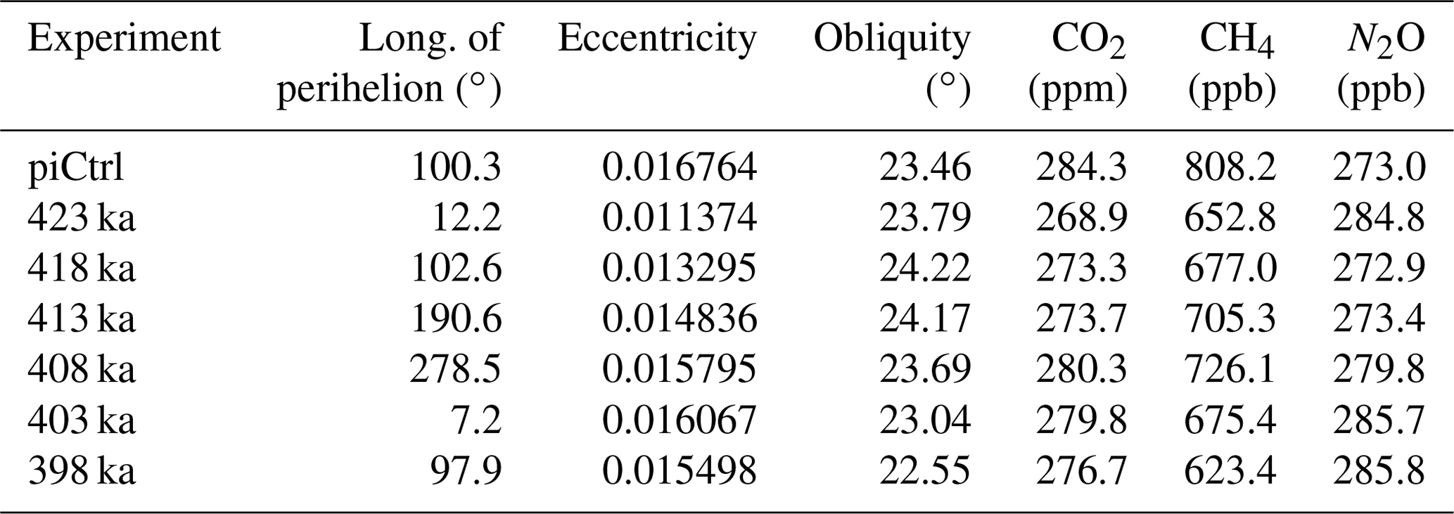
For each experimental simulation, orbital parameters were calculated following Laskar et al. (2004) at the representative time period. Greenhouse-gas concentrations were obtained from the European Project for Ice Coring in Antarctica (EPICA) record, primarily consisting of data from Dome C (Siegenthaler et al., 2005; Lüthi et al., 2008). Following the experimental setup detailed in Otto-Bliesner et al. (2017), a nominal +23 ppb adjustment was applied to Antarctic CH₄ values, accounting for the fact that methane persistently exists in higher concentrations in the Northern Hemisphere during interglacials. GHG values represent means of a 5 kyr window around the representative time (i.e., 423 ka GHG values are given by a mean of all values between 425.5 and 420.5 ka), which accounts for the inherent uncertainty in GHG values due to short-term variability (centennial and millennial scale) and the analysis techniques.

A sensitivity experiment was also conducted to ensure that the results of the time slice experiments were not dependent upon initialization. To this end, additional simulations for 418 ka were conducted, branching from year 500 of the preindustrial control run and from year 500 of the 423 ka run. A comparison of the equilibrated periods (final 100 years of each integration) showed that no statistically significant differences existed between them.

2.3 Statistical techniques

A number of correlation plots are presented in the results section. These present Pearson's r values, 95 % confidence intervals of the r values, and p values. Pearson's r is calculated with respect to the mean values of given quantities for each particular time slice. On interannual timescales, regional temperatures, eddy heat fluxes, etc. are noisy and influenced by a number of different factors. The most prudent comparison is therefore between the long-term mean patterns in each time slice simulation. When correlating 2 m air temperature and precipitation for all MIS-11 experiments, for example, the values correlated consist only of the six mean seasonal precipitation values from the time slices and the six mean seasonal temperature values from the time slices. The n for these correlations is therefore only six, and the degrees of freedom just four. In reality, 600 total seasonal values likely have a much greater number of degrees of freedom, although each time slice's 100 years of data is best classified as a red-noise time series and therefore does not have a full 100 degrees of freedom (Thomson, 1982). The significance of the correlations presented are therefore conservative.

Student's t tests are also employed to determine whether climatological changes between the time slice simulations and the preindustrial simulation are significant. For all variables tested, the seasonal values at each grid point and in each time slice are treated as an independent time series (n=100). This necessarily assumes spatial independence of each grid point. Critical values and p values are then obtained based on the effective degrees of freedom of each time series, reduced from 100 based on the lag-1 autocorrelation. The inherent assumption of normally distributed, spatially independent variables is not fully applicable for spatially coherent, non-normal variables like wind, eddy heat flux, and precipitation, but degrees of freedom are sufficiently large in all cases to ensure that t testing retains some explanatory power (Decremer et al., 2014). The 95 % confidence threshold presented in all figures here should not be considered as absolute, but an approximate representation of where anomalies are noteworthy.

3 Results

3.1 Surface temperature response

The surface temperature response is the most obvious effect of the varying orbital and GHG conditions throughout MIS-11 (Fig. 1). Global-mean 2 m air temperatures were at or modestly above preindustrial levels for each of the 423–408 ka simulations (dark blue). As expected, the temperature pattern is considerably amplified over Greenland, with positive anomalies reaching 2–3 ^∘C above preindustrial during the warmest period (413 ka). This result generally aligns well with the temperature anomalies over Greenland from two other recent studies utilizing EMICs for transient simulations of MIS-11. First, an ensemble of coupled REMBO-SICOPOLIS simulations with transient ice sheets was performed by Robinson et al. (2017), depicted in the gray line and shading in Fig. 1. Their simulations in turn rely on temperature anomalies derived from a transient climate simulation from the CLIMBER2 EMIC (Ganopolski and Calov, 2011). Our simulations deviate significantly from the these at the first time slice (423 ka), and to a lesser extent at 418 ka. This is most likely a result of our simulations assuming a fixed ice modern-day Greenland ice sheet, whereas the transient simulations still had greater Greenland and North American ice coverage from the previous glaciation. This is affirmed by further comparing our simulations to those of Yin et al. (2021), who utilized LOVECLIM1.3 with transient orbital and GHG forcing, but fixed present-day ice sheets. Near-surface air temperatures from their simulations (light red in Fig. 1) averaged around Greenland match our results very closely, including at 423 ka. Except for the discrepancies at 423 ka, differences between the fixed ice and fully transient simulations are otherwise minimal during MIS-11.

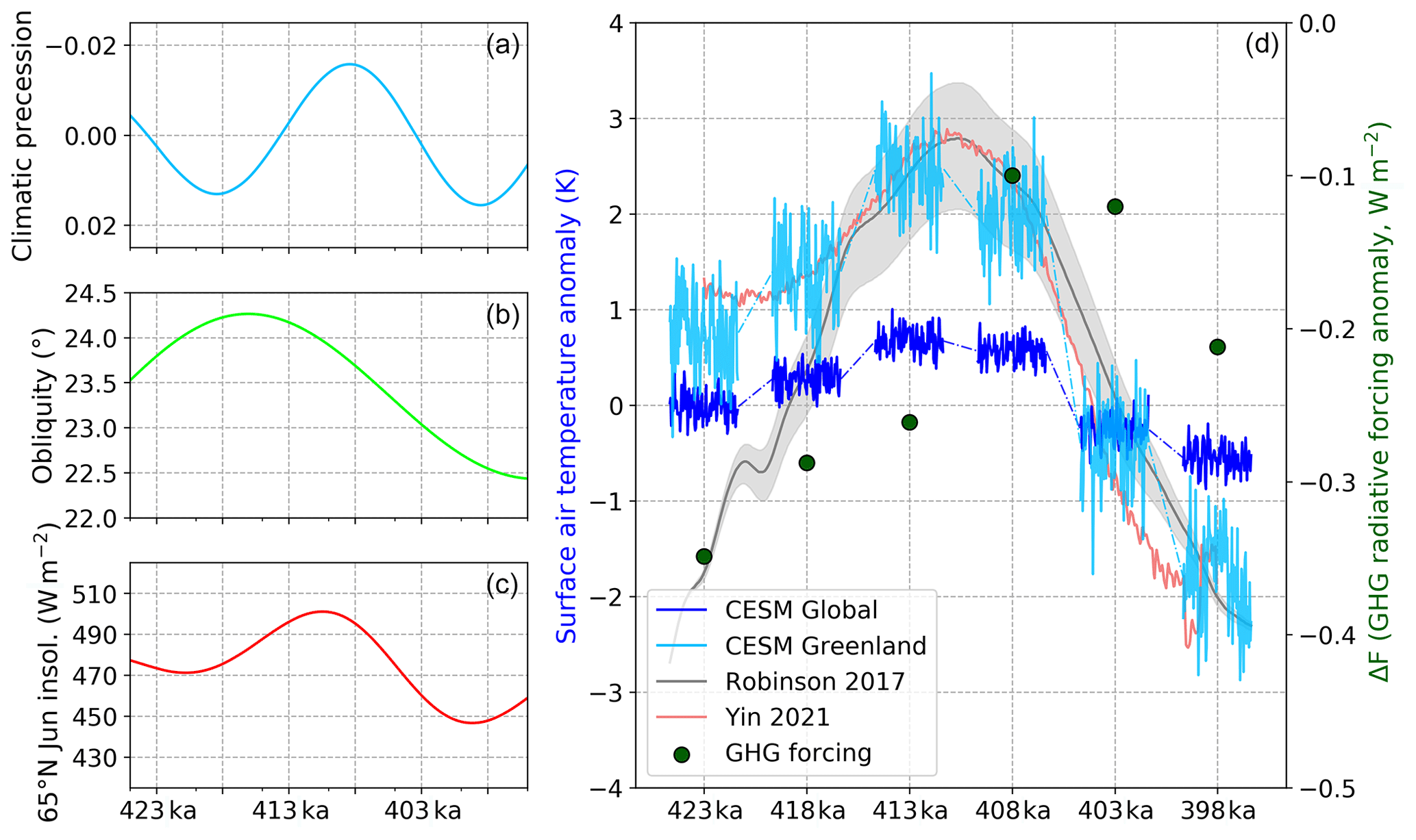
Figure 1 (a–c) Orbital parameters and high-latitude summer insolation during the MIS-11 interglacial. (d) Mean boreal summer global and area-weighted mean Greenland (55–85^∘ N, 280–350^∘ E) 2 m air temperature anomaly “pseudo-time series” relative to the preindustrial control simulation are given by the dark blue (global) and light blue (Greenland) curves. The pseudo-time series depict seasonal-mean boreal summer (June–July–August; JJA) values from the final 100 years of each simulation; the time x axis is therefore not to scale for these curves and the discontinuities are larger than depicted. The gray curve is the time series of JJA mean temperatures over Greenland from Robinson et al. (2017), which is based on an ensemble of transient, coupled REMBO-SICOPOLIS simulations; the surrounding gray shading represents the 95 % confidence interval for temperatures based on this ensemble, while the solid line represents the likeliest estimate. The light red curve is the temperature time series for the Greenland region from the fixed ice LOVECLIM simulation of Yin et al. (2021). The green dots in the right panel indicate the radiative forcing anomaly based on the combined effects of CO₂, CH₄, and N₂O, after IPCC (2001).

Figure 2 Mean JJA 2 m temperature anomalies for the final 100 years of each CESM simulation corresponding to the listed time slices. Regions with stippling pass Student's t test at the 95 % significance level. The green box in the 423 ka panel indicates the averaging region for the mean temperature values used in Fig. 1 and in the correlation plots (Figs. 4 and 7), 55–85^∘ N and 280–350^∘ E. The mean anomaly value listed beneath each panel is a cosine-weighted mean value of the complete shaded area (0–87^∘ N, 270–40^∘ E).

The spatial distribution and magnitude of boreal summer temperature anomalies across the North Atlantic sector also varied notably throughout the analysis period (Fig. 2). Anomalies as high as 4–5 ^∘C above preindustrial are evident around northern Greenland and the Canadian Arctic during the peak warmth of 413–408 ka due to the combined effects of high insolation and regional feedback, including reduced sea-ice cover (not shown). More modest and relatively uniform warming is present across much of the rest of the Atlantic basin, with the exception being areas immediately surrounding the Mediterranean Sea. A narrow but stark band of 1–2 ^∘C cool anomalies stands out in sub-Saharan Africa during the 423 and 413–408 ka simulations, the result of increased cloud cover and surface cooling induced by evaporation associated with enhanced monsoonal and intertropical convergence zone (ITCZ) convection. Also evident is the abrupt return of surface air temperatures to near-preindustrial conditions by 403 ka and substantial cool anomalies by 398 ka, consistent with conditions potentially favorable for renewed glaciation.

Inevitably, these results contain some bias introduced by using a fixed modern-day Greenland ice sheet in the simulations. In addition to the aforementioned warmth at 423 ka, temperature anomalies are likely somewhat underestimated over Greenland itself for later analysis periods, as the lowering and partial removal of ice surfaces would have enabled even warmer conditions. Additionally, changes in Greenland topography may also induce further warming on local to regional scales due to katabatic winds (Merz et al., 2014). These potential biases are particularly relevant for the 413–398 ka time slices, when the ice sheet was likely smaller than the present day.

Regardless of the exact magnitude of summer warming during MIS-11, the signal for large, statistically significant warming at high latitudes is robust. One clear consequence of strong warming at high latitudes, especially when paired with tropical surface cooling over Africa, is the reduction of the mean Equator-to-pole surface temperature gradient, and thus the contribution of the thermal wind balance to the geostrophic flow. A dynamic adjustment of baroclinic processes is therefore to be expected, including attendant changes in jet stream and baroclinic eddy behavior.

3.2 Atmospheric eddy response

Particularly robust changes are present in the lower-tropospheric meridional eddy heat flux (EHF) anomalies across the North Atlantic sector. Note that future references to baroclinicity, meridional temperature gradients, or eddy heat fluxes in this text are concerning only lower-tropospheric quantities, and EHF in general refers to the meridional flux of heat by atmospheric eddies. Figure 3 illustrates the mean patterns of total (transient plus stationary) boreal (sensible) summer eddy heat flux anomalies relative to the preindustrial control simulation. Stationary eddy heat fluxes are defined as $\stackrel{\mathrm{‾}}{v^{\ast }}\stackrel{\mathrm{‾}}{T^{\ast }}$, where v^∗ and T^∗ are the zonally anomalous meridional wind and temperature, respectively, with anomalies calculated at daily intervals and at the 700 hPa atmospheric pressure level before being averaged to seasonal values. Transient eddy heat fluxes are likewise defined as $\stackrel{\mathrm{‾}}{v^{\prime }{T}^{\prime }}$, or the product of the time-anomalous meridional wind and temperature. The total EHF is simply the sum of the transient and stationary meridional eddy heat fluxes and is, in effect, representative of the heat-advecting effects in the lower-to-middle troposphere of the atmospheric waves captured in the model. Over the large majority of the analysis domain, total meridional EHF anomalies are dominated by the transient eddy component (not shown). The values represented in the figure are averages of all the June–July–August (JJA) days in the 100-year period, relative to the preindustrial simulation.

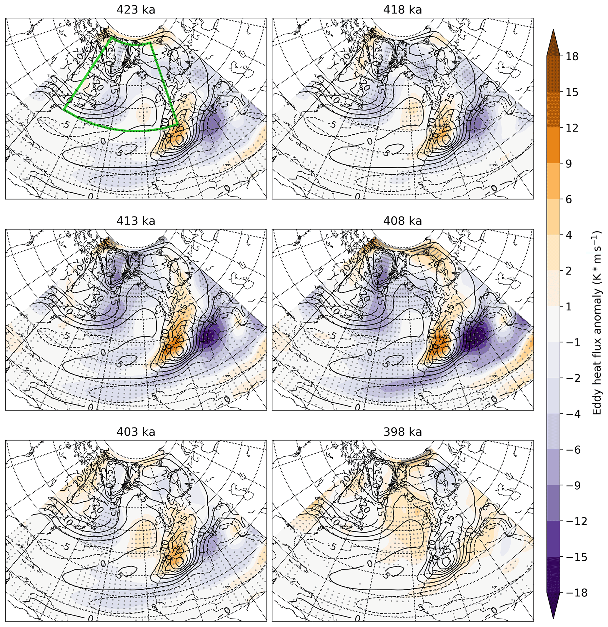
Figure 3 Mean lower-tropospheric (700 hPa) total eddy heat flux anomalies over the North Atlantic. Black contour values indicate the mean JJA total eddy heat flux from the final century of the piCtrl run (baseline climatology). Shaded values shown are boreal summer mean anomalies over the final 100 years of each designated simulation, stippled where the difference is statistically significant at the 95 % level. The green box in the 423 ka panel shows the area (40–80^∘ N, 290–0^∘ E) over which area-mean values are computed for correlations in Figs. 4 and 8.

Two features in the total meridional EHF anomaly fields stand out. First, the couplet of positive and negative anomalies over southwestern Europe and the central Mediterranean during 423–408 ka is indicative of a robust shift in the favored storm track. Positive EHF anomalies are indicative of either an increased and anomalous meridional temperature gradient or frequent large southerly wind anomalies (transient or stationary), or more likely, some combination thereof. Given that the mean temperature gradient appears unchanged or even slightly weaker (Fig. 2), the likely source of this anomaly is increased frequency and/or intensity of wave activity and meridional transport in this region. Conversely, reductions exist over the central Mediterranean, consistent with a shift in baroclinic wave activity away from this region. Considered together, the strong anomaly couplet (for all periods except 398 ka) over Europe and the Mediterranean represents a northwestward shift in the mean storm track over the eastern Atlantic.

A second region of widespread and statistically significant reduction in total eddy heat fluxes is present over much of Greenland and the open North Atlantic. The magnitude is overall smaller than the anomalies over Europe and the Mediterranean, but rather than marking a simple shift or intensification of the preindustrial pattern, it appears to resemble an entirely different wave pattern. Meridional heat flux from eddies is clearly reduced in the MIS-11 simulations (except 398 ka) in a broad area extending from the Canadian Maritime Provinces up through much of Greenland, a region that experiences relatively large meridional EHF in the preindustrial mean (black contours in Fig. 3). As will be discussed in Sect. 3.3, this is a clear indication of an altered storm track across the North Atlantic.

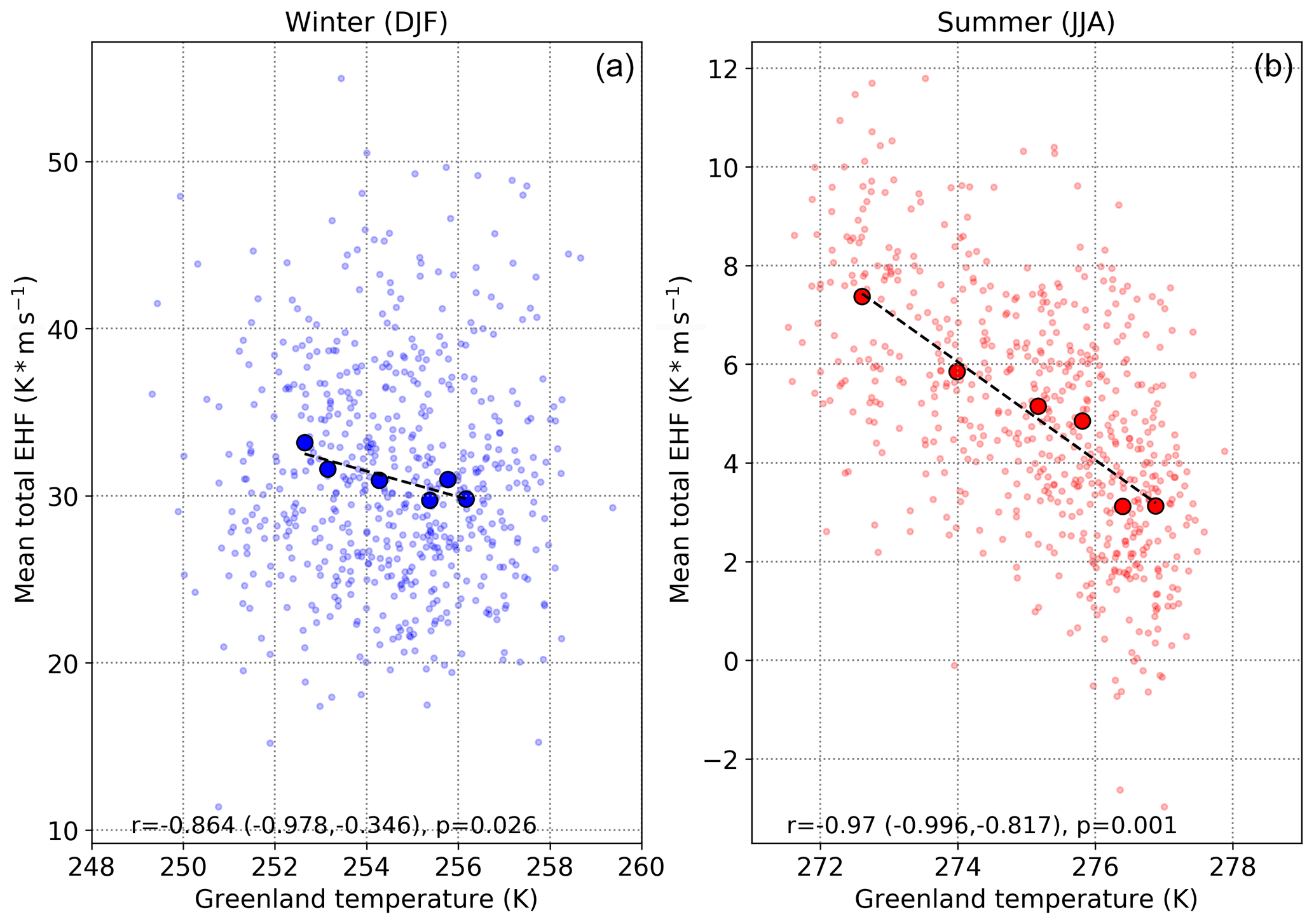
Figure 4 Correlations between the mean surface air temperature around Greenland (55–85^∘ N, 280–350^∘ E) and the seasonal-mean total (stationary + transient) eddy heat flux over the North Atlantic (40–80^∘ N, 290–0^∘ E). Correlations, p values, and trend lines are calculated using mean values of temperature and EHF anomalies for each of the six time slices. Individual years are lightly colored small dots, and the mean of each of the six time slice simulations are given by large, outlined dots.

As implied by comparing the eddy heat flux and surface temperature maps, a strong negative correlation exists between the temperature averaged over Greenland and its immediate surroundings (the region enclosed by the green box in the top-left panel of Fig. 2) and the mean eddy heat flux over the North Atlantic region (the larger region enclosed by the green box in Fig. 3). The strength of this relationship is also strongly dependent on the season (Fig. 4). While both boreal winter-mean and summer-mean EHF–temperature relationships exceed the 95 % confidence threshold, the correlation is much stronger and has a much narrower confidence interval in boreal summer. This can be partly explained by the much larger magnitude and variability of seasonal-mean North Atlantic eddy heat fluxes in winter, but is also indicative of a more robust dynamic response in the summer season.

3.3 Jet stream response

While reduced meridional temperature gradients play a role in reducing eddy heat fluxes, changes in eddy activity are the dominant cause. Eddy activity in the midlatitudes has a symbiotic relationship with the jet stream, which both drives and is driven by wave activity. An attendant change is therefore expected in jet behavior, which is apparent in the daily jet frequency matrices (Fig. 5). A clear shift in the favored latitude and strength of the boreal summer North Atlantic jet is evident, with weaker and lower-latitude daily maximum 300 hPa winds clearly favored in the 418, 413, and 408 ka experiments. These three warm periods also show a slight reduction in the frequency of low-latitude jet maxima, denoted by the slight negative frequency anomalies on the lower flank of the robust couplet. This is consistent with a decreasing tendency towards wind maxima in the typical (modern) latitude of the subtropical jet, an observation which is further supported by the presence of negative mean 300 hPa wind anomalies (Fig. 6).

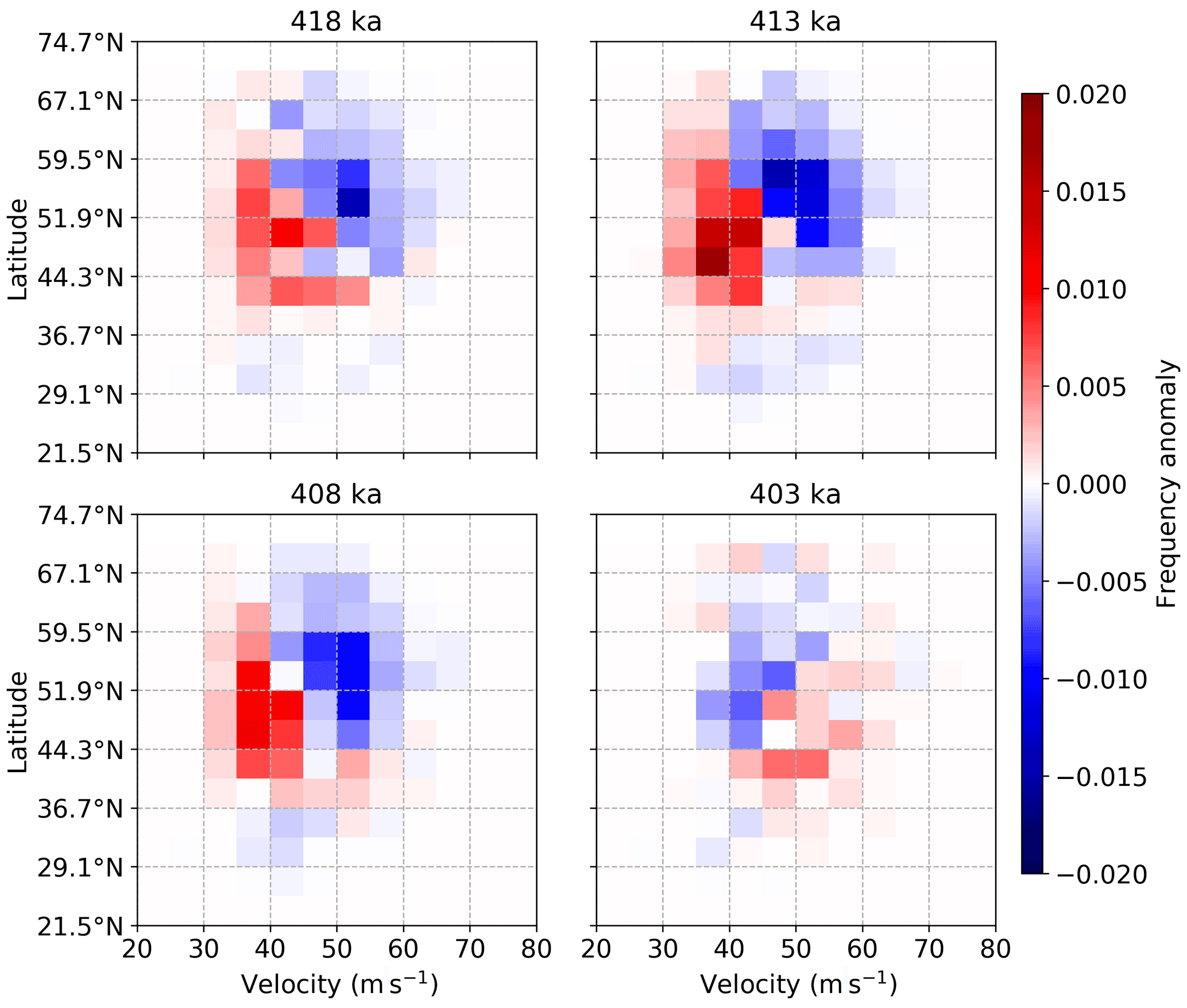
Figure 5 Changes in the frequency of the latitude and peak velocity of JJA daily maximum 300 hPa winds over the North Atlantic for the core MIS-11 interglacial period of 418–403 ka. Latitude bins are approximately 3.8^∘, containing two model grid cells each. Velocity bins are at intervals of 5 m s⁻¹. Frequency matrices are computed relative to the preindustrial control simulation, and the velocity maxima reflect the maximum single value at any grid point in the analysis domain.

Figure 6 Mean JJA wind anomalies at 300 hPa across the MIS-11 simulations (colors) and climatological 300 hPa wind velocities from the piCtrl simulation (black contours). Anomalies significant at the 95 % level via t testing are stippled. Evident reductions in mean winds across both the typical subtropical jet location (∼ 25–35^∘ N) and the typical polar jet location (∼ 50–70^∘ N) are present in most time slices, along with increases in mean winds across the eastern midlatitude North Atlantic and western Europe.

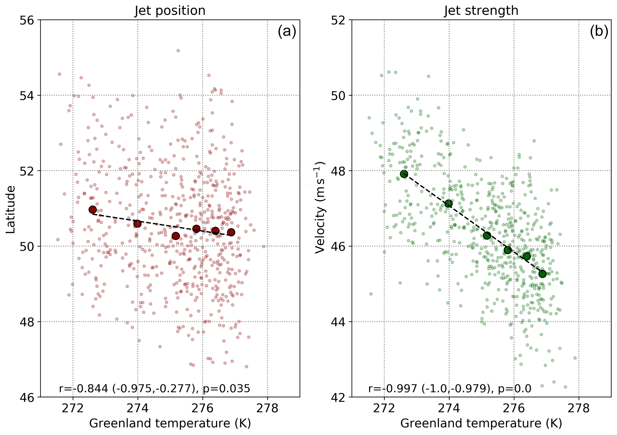
Figure 7 The relationships between the JJA-mean Greenland (55–85^∘ N, 280–350^∘ E) 2 m air temperature and the latitude (a) and magnitude (b) of maximum 300 hPa winds across the North Atlantic. As in Fig. 4, correlations, best-fit lines, and p values are calculated with respect to the overall means of each time slice (indicated by large, outlined dots). The smaller dots represent the seasonal-mean values for each of the 100 years of each time slice.

Thus, both purely eddy-driven high-latitude jet maxima and purely subtropical jet maxima are reduced (the southern flank subtropical wind weakening is even more clearly visible in the u component of the wind field; not shown), with the dominant state instead emerging as a broad hybrid eddy–thermal jet in the midlatitudes. Son and Lee (2005) used an idealized aquaplanet model simulation to demonstrate that either weakened midlatitude baroclinicity or stronger tropical ascent could cause the jet to transition to a unified state. Interestingly, both mechanisms are present during MIS-11 boreal summers in our considerably more realistic simulations. As discussed in Sect. 3.1, baroclinicity changes are clear in the temperature anomaly patterns (Fig. 2) and additionally implied by the robust negative correlation between jet strength and mean 2 m air temperature over the North Atlantic (Fig. 7). As will be discussed further in Sect. 3.5, the band of tropical cooling over Africa is a result of increased convection, cloud cover, and evaporative surface cooling, thus indicating enhanced tropical ascent.

3.4 Eddy–jet relationship

Notably, the region with the large couplet in EHF anomalies over western Europe and the Mediterranean (Fig. 3) corresponds approximately with the largest changes in jet stream wind strength (Fig. 6). Since the changes in EHF are dominated by the transient component, it is clear that the emergence of these anomalies is associated with a significantly altered North Atlantic storm track. A more baroclinically active JJA storm track across this region appears to be the consequence of the merged jet state, which is also consistent with the trapping of atmospheric waves equatorward of a merged jet (e.g., Nakamura and Sampe, 2002). Reduced baroclinic eddy activity on the poleward flank of the merged jet explains the existence of the opposite state (reduced EHF) across much of the open North Atlantic. The contrast is made clear by examining the 300 hPa wind (Fig. 6) and total eddy heat flux maps (Fig. 3). During 423–403 ka, large reductions in EHF are present across the central and North Atlantic in association with the weakened polar jet to varying degrees; in cooler-than-preindustrial 398 ka, these have been replaced by small positive anomalies in association with the return to a split-jet state.

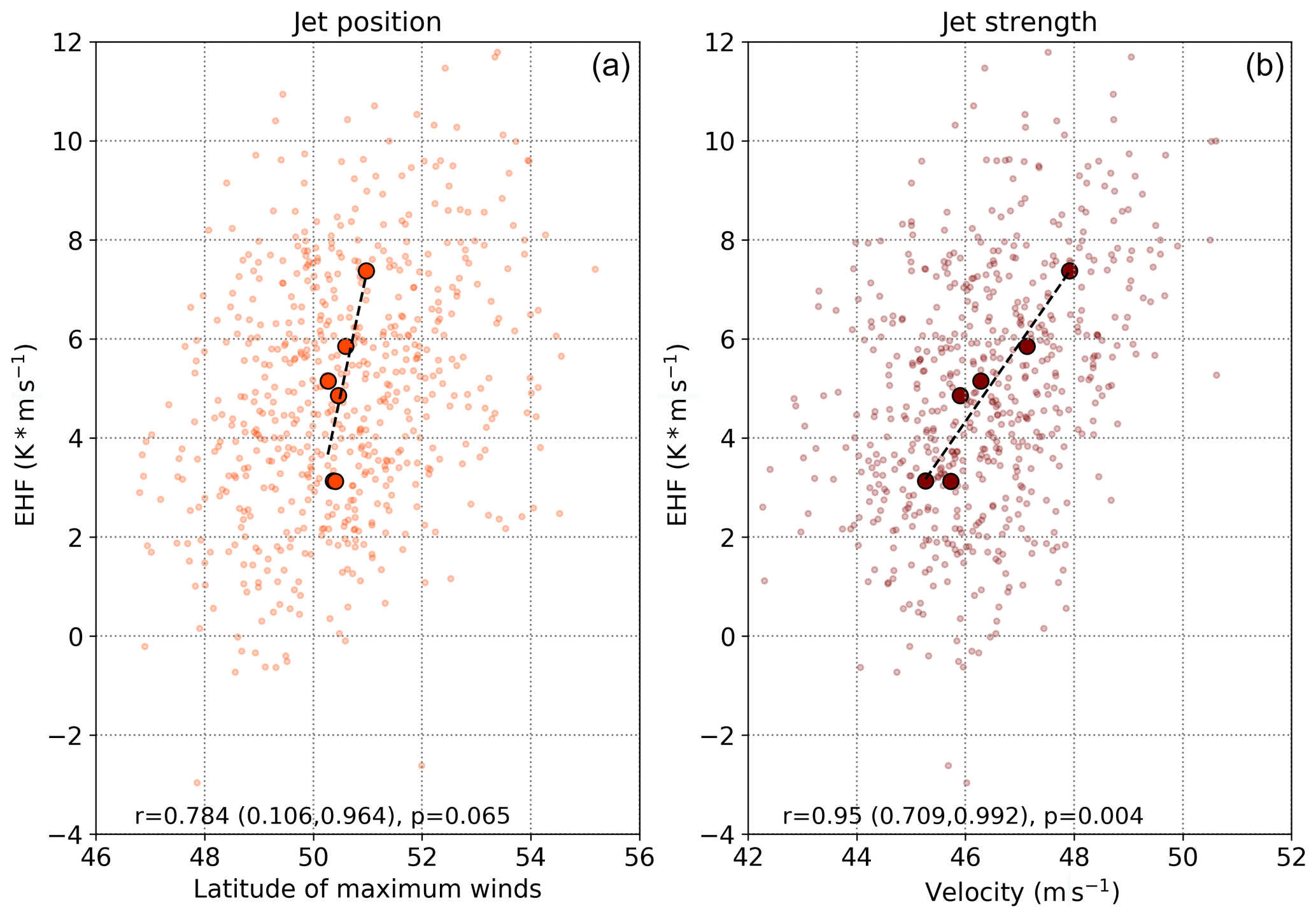
Figure 8 Correlations between summer mean seasonal values of the latitude of maximum 300 hPa winds (a), the magnitude of jet maximum winds (b), and total eddy heat flux over the North Atlantic (40–80^∘ N, 290–0^∘ E). Correlation does not reach 95 % significance for jet position, but the correlation with jet strength is robust.

Interestingly, correlations between EHF anomalies and jet characteristics fail to paint quite so clear a picture. While hints of a relationship between jet latitude and North Atlantic-mean EHF (mean over a box spanning 40–80^∘ N and 70^∘ W–0^∘ E) exist, the correlation does not reach significance at the 95 % confidence level (Fig. 8). However, EHF exhibits a strong positive correlation with boreal summer jet strength in the North Atlantic. Our simulations indicate that split-jet states are associated with higher absolute maximum jet strengths. Therefore, the strong positive correlation between higher maximum jet velocities and North Atlantic meridional EHF implies greater EHF during split-jet regimes, and reduced EHF during the prevailing merged-jet regime of MIS-11 boreal summers.

3.5 Precipitation and the storm track

Precipitation across the Greenland ice sheet is highly seasonal, predominantly driven by extratropical cyclones, and strongly enhanced along major orographic features, particularly in the southeast (Chen et al., 1997). With such a pronounced change in eddy behavior (extratropical cyclones) as a result of the shifted jet, a logical consequence would seem to be a positive correlation between jet strength and precipitation over Greenland. However, exactly the opposite appears to be the case (Fig. 9), with a significant but small negative trend in precipitation associated with higher North Atlantic wind maxima based on time slice means. A considerable amount of noise exists among the individual annual values, however, so this result should be treated with some caution. As is the case with the EHF correlations (Fig. 8), only the relationship between maximum jet velocity and precipitation obtains 95 % significance.

Figure 9 Relationships between JJA-mean latitude of maximum 300 hPa winds (a), the magnitude of the maximum jet wind (b), and seasonal-mean precipitation over Greenland (land-only). As with eddy heat fluxes, the correlation is only significant for jet strength.

Competing effects appear to be influencing precipitation over Greenland in these simulations: intuitively, increases in eddy heat flux should correspond to increases in eddy moisture flux (EMF). However, comparing the jet state to total EMF over the North Atlantic directly results only in a statistically insignificant correlation (not shown). On the other hand, we have demonstrated that warmer North Atlantic temperatures are associated with weaker jets, and lower-tropospheric air temperature places a strong cap on atmospheric moisture. The apparent negative correlation between maximum jet winds and precipitation over Greenland (Fig. 9) therefore appears to be overwhelmingly driven by the inverse relationship between temperatures over Greenland and jet strength. Behavioral changes in the jet and eddies exhibit only a secondary influence.

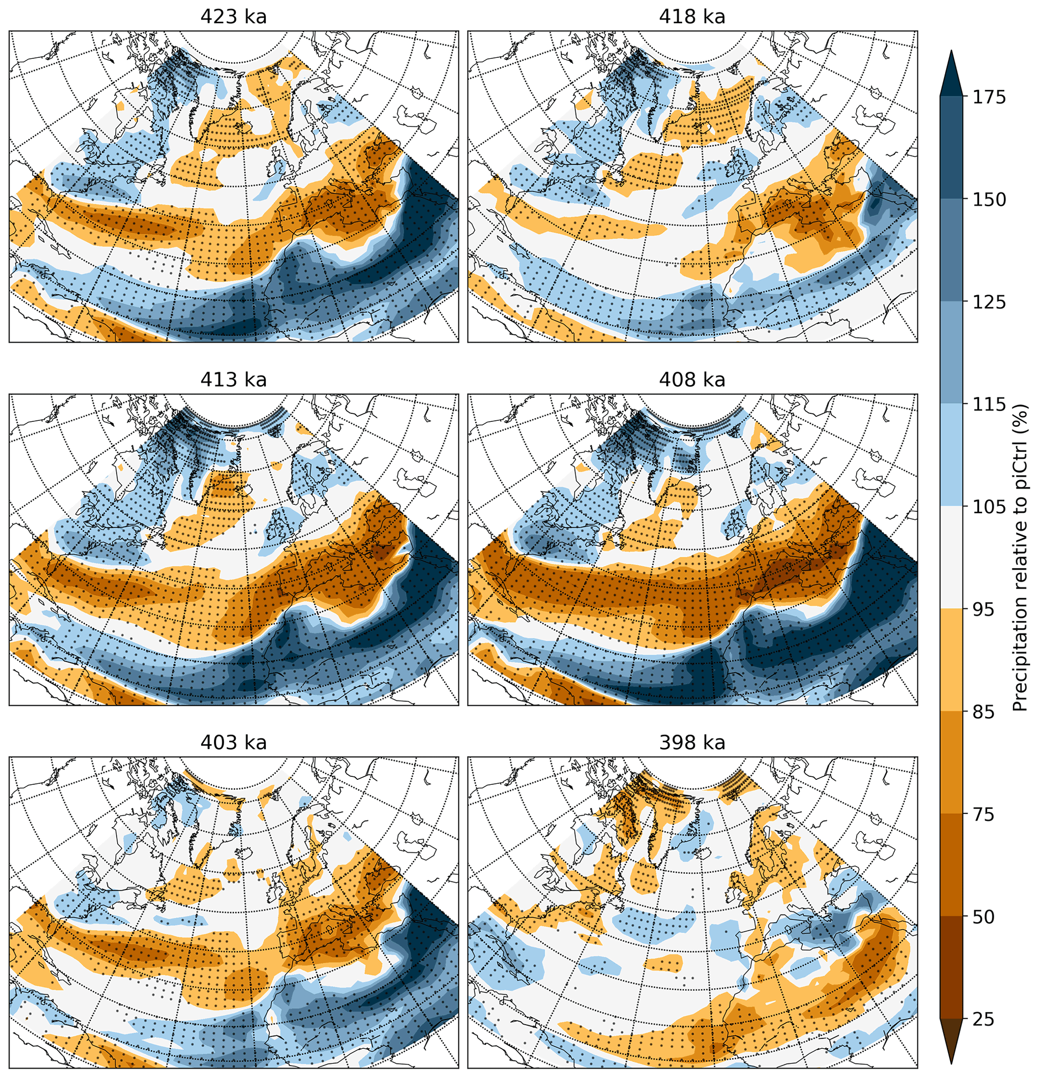
Figure 10 Time slice mean summer precipitation anomalies across the North Atlantic throughout MIS-11, indicating slight increases in precipitation on the western slope of Greenland with corresponding decreases in the southeast from 423 to 408 ka. Stippled regions correspond to grid points significantly different from the preindustrial control simulation at the 95 % confidence level.

Spatially, the largest boreal summer precipitation changes across the analysis domain appear to be related to the strength of the African monsoon (Fig. 10). Specifically, a drying is noted across much of the midlatitude Atlantic and much of central and southern Europe, consistent with the general shift of the preferred storm track and suggestive of increased subsidence from the poleward flank of the Hadley cell. The magnitude of subtropical drying appears to be roughly proportional to the increase in precipitation over sub-Saharan Africa, strongly suggesting the influence of tropical convection on the altered jet state. Precipitation increases across west/central Africa associated with the increased monsoon are evident through the 423–403 ka periods, peaking at over 175 % of preindustrial under 408 ka conditions. Attendant decreases of around 5 %–25 % over Europe, 25 %–50 % for most of the Mediterranean, and 5 %–25 % across the Caribbean and western subtropical Atlantic are also evident during 413 and 408 ka. The largest monsoon precipitation increases appear to occur at 418 and 408 ka, roughly corresponding with the periods of most negative precession (perihelion occurring near/during boreal summer).

Figure 11 As in Fig. 10, but for the annual mean period.

Over Greenland, boreal summer precipitation changes during the warm 423–408 ka period resemble that of orographic precipitation during dominant westerly/northwesterly wind regimes: positive precipitation anomalies along the western slopes and negative anomalies along and just off the southeastern coast. In absolute terms, these anomalies are relatively small, on the order of 0.1–0.3 mm d⁻¹, but constitute statistically significant 5 %–25 % increases. In the annual mean, however, a near-opposite pattern emerges in precipitation anomalies for southeastern Greenland (Fig. 11). Simulated annual average precipitation rates increase there by 5 %–15 % for the 418–408 ka period. Since the bulk of the southeastern Greenland precipitation increase occurs in the cool season, it occurs overwhelmingly as snow (not shown but confirmed by model precipitation-type output), and therefore contributes to an increase in the mass balance of the ice sheet across southeastern regions.

4 Discussion

Our results compare favorably with the limited previous modeling studies conducted to assess MIS-11 climate. The same pronounced high-latitude warming and narrow region of tropical cooling identified in our study with CESM was also found by Kleinen et al. (2014) in both an EMIC (CLIMBER2) and an AOGCM (CCSM3), suggesting a signal robust to various climate models. Likewise, they identified the enhancement of the African monsoon and the migration and strengthening of tropical convection over the eastern Atlantic, albeit with a more limited spatial extent of increased precipitation than in our simulations. Further analysis of the same two CCSM3 time slices in Rachmayani et al. (2016) confirmed these temperature and precipitation relationships.

The consensus among recent climate modeling studies therefore indicates a robustly strengthened African monsoon during MIS-11 in boreal summer. Despite severe limitations in the availability and spatial coverage of reliable proxy records from this time period, the data that exist appear to support this. Decreased deposition of terrigenous iron in the deep ocean off the coast of northwestern Africa during the period 420–396 ka indicates a substantially less dusty (i.e., wetter) northwest African climate during this time (Helmke et al., 2008). Also coincident with this development was the occurrence of increased deposition of organic matter in the eastern Mediterranean (sapropel 11), approximately dated to 407 ka and likely the result of increased freshwater input from the Nile River as eastern African rainfall increased (Kroon et al., 1998; Lourens, 2004). Timing the African wet period to a resolution greater than a few thousand years or determining precisely the magnitude of the rainfall changes is still beyond the precision afforded by these records; however, they do offer some general verification of the signal produced by the model consensus.

Primary responsibility for the changes in both the African monsoon and the midlatitude baroclinicity naturally lies with the insolation changes. Both inter-hemispheric and intra-hemispheric changes to the insolation gradient have roles to play, with the relatively high obliquity conditions of the early–middle MIS-11 interglacial (ca. 423–408 ka) a chief contributor to the lower-tropospheric low-baroclinicity conditions in boreal summer. High obliquity conditions are responsible for increased high-latitude insolation in the summer hemisphere, thus driving the reduction in the meridional surface temperature gradient seen in our simulations (Mantsis et al., 2014). Furthermore, high obliquity enhances the inter-hemispheric temperature gradient, sustaining a stronger Hadley circulation and causing a poleward shift in the Hadley cell in the summer hemisphere (Mantsis et al., 2014). Climatic precession is known to have the dominant effect on the state of the north African monsoon (e.g., Bosmans et al., 2015), which is illustrated in our simulations by the emergence of the strongest monsoon conditions during 408 ka (and, conversely, the weakest monsoon precipitation anomalies nearest precession maxima at 418 and 398 ka). The favorable alignment of moderate–low precession and moderate–high obliquity throughout much of MIS-11 thus produces sustained Northern Hemisphere boreal summer warmth as well as monsoon and jet responses over an anomalously long period.

As others have noted, the changes in baroclinicity seen during MIS-11 will likely be mirrored to some extent by present and future GHG-induced global warming, suggesting the possibility of a strengthened African monsoon and northward-shifted Atlantic ITCZ in the not-so-distant future (Mohtadi et al., 2016, and references therein). In the present climate, it has been demonstrated that an improved understanding of western African convection can significantly improve weather forecast skill across Europe and the North Atlantic due to teleconnection patterns (e.g., Pante and Knippertz, 2019). Long-term and large-scale mean circulation anomalies in the west African monsoon region thus have far-reaching implications for regional or global weather and climate patterns, including over Greenland. Improved understanding of the two-way dynamic linkages between patterns of tropical convection during boreal summer and changes in the North Atlantic circulation are necessary in order to optimize predictions of future Greenland ice sheet behavior.

It also remains to be determined to what extent the jet–eddy response identified here is robust to all models, given the variable degree to which the North Atlantic storm track tends to be southward-biased in Climate Model Intercomparison Project (CMIP) models (Harvey et al., 2020). Numerical models can also struggle to replicate the magnitude and latitudinal extent of the west African monsoon circulation, which, given the sensitivity of the midlatitude jet to tropical forcing in our simulations, suggests another potential bias of concern (e.g., Brierley et al., 2020). Our study also does not test the sensitivity of the jet–eddy response to varying levels of GHGs under identical orbital forcings, which are subject to some uncertainty for paleo-periods like MIS-11 given millennial-scale fluctuations and the relatively low temporal resolution of GHG records (variable between a few hundred and approximately 1000 years). Natural limitations on the availability of quality reconstructions will almost certainly continue to prevent true “validation” of modeling results as well.

The use of a fixed modern-day Greenland ice sheet in our climate simulations represents probably our most significant assumption, although the effects of this are less important in the summer than in the winter (Merz et al., 2014). Elevation reductions on the order of several hundred meters across the GrIS would result in 2 m air temperature increases of several degrees Celsius, further enhanced by albedo reductions due to the melting of the ice sheet and emergence of bare rock, soil, and vegetation across marginal regions. In fact, modeling sensitivity studies examining future scenarios have identified these factors as contributing to notably larger GrIS ablation areas and sea-level rise from Greenland melt when accounted for in a two-way coupled simulation (Le clec'h et al., 2019). Failure to account for the increased freshwater discharge from the ice sheet in periods of substantial melt may also affect local ocean circulations and sea-ice formation, which can in turn feed back into Greenland air temperatures and local atmospheric circulation (e.g., Merz et al., 2016). It is also possible that these feedback mechanisms may result in further reduced baroclinicity across the North Atlantic sector, possibly further reinforcing the unified-jet state and leading to additional reductions in eddy heat fluxes.

Competing effects on precipitation are also possible: increased atmospheric moisture content is expected over a warmer, lower-elevation Greenland surface; however, the diminished topography in large sections of Greenland would be expected to reduce the production of orographically induced precipitation. We plan to investigate the dynamic atmospheric response to a greatly reduced GrIS under MIS-11 climate conditions in a future sensitivity study, and thus hope to better assess the appropriateness of the fixed ice sheet assumption.

5 Conclusions

Using CESM time slice simulations of only insolation and GHG forcing conditions corresponding to the MIS-11 interglacial, we have uncovered a robust dynamic atmospheric response that includes negative feedback to further melting of the Greenland ice sheet. Increased high-latitude insolation due to a favorable alignment of high obliquity and relatively low-amplitude climatic precession variations across a time interval of around 20 kyr drives pronounced, sustained boreal summer surface warming across Greenland and the surrounding high-latitude oceanic regions. It remains a future task to determine if this insolation-driven surface warming alone is sufficient to produce GrIS melt of the magnitude proposed by previous studies (e.g., Alley et al., 2010; Reyes et al., 2014; Robinson et al., 2017). Resolving this question is complicated by the two negative feedback mechanisms we have identified in the atmospheric response to MIS-11 interglacial forcing: (i) a transition in preferred jet stream behavior leading to reductions in poleward eddy heat flux over the Greenland sector, and (ii) increased annual-mean precipitation over the ice sheet. The mass balance implications of these feedback mechanisms will be explored in a planned future ice sheet modeling study.

The preferred boreal summer jet response to MIS-11 forcing identified here, driven by the combined effects of weakened midlatitude baroclinicity and enhanced tropical ascent over the Atlantic sector, is more consistent with the merged-jet state considered to be characteristic of glacials rather than interglacials (e.g., Andres and Tarasov, 2019; Merz et al., 2015). Further study, and comparison with other interglacial climate simulations, may clarify whether this is a unique feature of MIS-11 or typical of strong interglacials. Earlier studies utilizing medium-resolution CCSM3 simulations (Herold et al., 2012; Rachmayani et al., 2016) suggest that an enhanced African monsoon and warmer high-latitude temperatures are typical features of late-Quaternary interglacial states, indicating that at least the primary mechanisms behind the jet changes tend to be present. However, spatial patterns of warming and the degree and duration of monsoon enhancement appear to vary considerably between interglacials, and it therefore remains to be seen whether the dynamic conditions present in other interglacials favor the same northern summer jet configuration.