the Creative Commons Attribution 4.0 License.
the Creative Commons Attribution 4.0 License.
 | 04 Mar 2022
Climate variability and grain production in Scania, 1702–1911
Martin Karl Skoglund
Scania (Skåne in Swedish), southern Sweden, offers a particularly interesting case for studying the historical relationship between climate variability and grain production, given the favorable natural conditions in terms of climate and soils for grain production, as well as the low share of temperature-sensitive wheat varieties in its production composition. In this article, a contextual understanding of historical grain production in Scania, including historical, phenological, and natural geographic aspects, is combined with a quantitative analysis of available empirical sources to estimate the relationship between climate variability and grain production between the years 1702 and 1911. The main result of this study is that grain production in Scania was primarily sensitive to climate variability during the high summer months of June and July, preferring cool and humid conditions, and to some extent precipitation during the winter months, preferring dry conditions. Diversity within and between historical grain varieties contributed to making this risk manageable.
Furthermore, no evidence is found for grain production being particularly sensitive to climate variability during the spring, autumn, and harvest seasons. At the end of the study period, these relationships were shifting as the so-called early improved cultivars were being imported from other parts of Europe. Finally, new light is shed on the climate history of the region, especially for the late 18th century, previously argued to be a particularly cold period, through homogenization of the early instrumental temperature series from Lund (1753–1870).
- Article
(6640 KB) - Full-text XML
- BibTeX
- EndNote


In recent years, numerous studies have explored the relationship between grain yields, prices, and climatic change in medieval and early modern Europe. The fundamental assumption underlying these studies is that grain production to a substantial degree was affected by variability in temperature and precipitation (Edvinsson et al., 2009; Holopainen et al., 2012; Camenisch, 2015; Esper et al., 2017; Pribyl, 2017; Ljungqvist et al., 2021a, b). Most of these studies have either focused on particularly temperature-sensitive grain types like wheat or temperature-sensitive agricultural regions, like Finland or the Scottish Highlands (Parry and Carter, 1985; Brunt, 2015; Huhtamaa and Helama, 2017a). In these historical contexts, cold conditions become the “grim reaper” (Holopainen and Helama, 2009). However, in the long term, grain farming even in the northern border regions of European agriculture has shown considerable adaptability and resilience (Solantie, 1992; Huhtamaa and Helama, 2017b; Degroot, 2021). Diversified grain production has been identified as an important aspect of this resilience (Michaelowa, 2001). In this article, I argue that an understanding of the impact of climatic variability and change on agriculture as well as explanations of resilience in terms of grain diversity need to be grounded in an understanding of the phenology of historical grain varieties.
Attempts to account for the resilience, or the ability of early modern farmers and farming systems to cope with climate variability in intensive grain farming areas of Europe north of the Alps like northern France and England, have remained mainly hypothetical (Michaelowa, 2001; Tello et al., 2017). Early modern Scania offers an especially interesting case in this regard. The climate of Scania is mild, hosting a continental climate stabilized by the proximity to the Baltic Sea. From an agronomic viewpoint, it is often stressed that Scania has the longest vegetative period of present-day Sweden (Osvald, 1959; Persson, 2015). Moreover, the southwestern half of Scania, roughly the extent of the historical county of Malmöhus, contains large areas of soils of exceptionally high quality (Lantbruksstyrelsen, 1971). For most of the historical period, Scania was an important surplus producer of grains in the Kingdom of Denmark and from 1658 in the Kingdom of Sweden (Åmark, 1915; Bohman, 2010). At the same time, since at least the 17th century up until the end of the 19th century, Scanian farmers relied on Scandinavian grain varieties adapted to cooler and humid climates with short growing seasons, i.e., conditions often prevalent at the northern limits of arable agriculture (Lundström et al., 2018; Larsson et al., 2019).
The aim of this article is to study the relationship between climate variability and grain production in Scania during the period 1702–1911. The study period is divided into the early study period (1702–1865) and the late study period (1865–1911). Given that the role of climate cannot be conceptualized in a simplistic or deterministic manner, it has to be contextualized in the specific agrarian and ecological context (Haldon et al., 2018; van Bavel et al., 2019; Degroot, 2021). Accordingly, this article starts out by contextualizing the study and setting the historical background, particularly detailing historical grain production in Scania during the study period. Following this is a conceptual and theoretical discussion of the relationship between crop production and climate as well as the concept of resilience. Subsequently, I present and discuss the climate and agricultural production data and the employed methods. Finally, results are discussed in relation to the historical context as well as to previous research.
1.1 Background
Scania is situated at the southernmost tip of the Scandinavian Peninsula in the borderlands between Sweden and Denmark. The farming districts on the plains of Scania have, and continue to be, some of the most productive arable farming regions in Scandinavia, owing mostly to its mild climate and rich soils. In the Danish and Swedish historiography, Scania is commonly referred to as a kornbod (roughly translated as “breadbasket”). Adam of Bremen in his Gesta Hammaburgensis ecclesiae pontificum from ca. 1075 CE describes Scania as the most prosperous of the provinces in the Danish kingdom (Bremensis, 2002). However, the natural geography of Scania is and was not uniform (Svensson, 2016). Besides the arable plains, Scania was constituted by a diverse landscape of forests, disparate but mostly hospitable coastal areas, lakes, and hills with different soils and natural conditions (Lidmar-Bergström et al., 1991). Farming was to some extent adapted to this variability in natural conditions, especially in the period prior to the late 19th century (Dahl, 1989; Gadd, 2000; Bohman, 2010). During the years ca. 1750–1850, Scania underwent what has been called the agrarian revolution, implicating a general transformation of agriculture as well as dramatic and sustained increases in production (Olsson and Svensson, 2010). Subsequently, Scanian agriculture has continued to sustain its growth trajectory, intermittently interrupted by various agrarian and economic crises (Myrdal and Morell, 2013). Scanian farmers also faced challenges. Situated between two rivalling kingdoms, Denmark and Sweden, the fertile plains of Scania have been fought over and acted as a battleground in numerous wars. After 1711, there were fewer conflicts compared to the preceding centuries (Frost, 2000).
Like in other parts of Europe, colder climatic conditions prevailed in Sweden and Scania for most of the second half of the 16th century and throughout most of the 17th century. The period ca. 1560–1630 was particularly cold and experienced overall increased climatic variability (see Fig. 1). In the 1690s, there was also a recurrent span of cold years with late springs in the Baltic area, culminating in the disastrous years of 1695–1697 and leading to mass mortality throughout the region, especially in northern Sweden, Estonia, and Finland (Dribe et al., 2015; Lilja, 2008). Reconstructions of winter ice severity from the western Baltic indicate that the period experienced greater volumes and persistence of winter ice compared to preceding and subsequent periods, and the sound between Scania and Zealand was covered with ice for most of the years 1694–1698 (Speerschneider, 1915; Koslowski and Glaser, 1999).
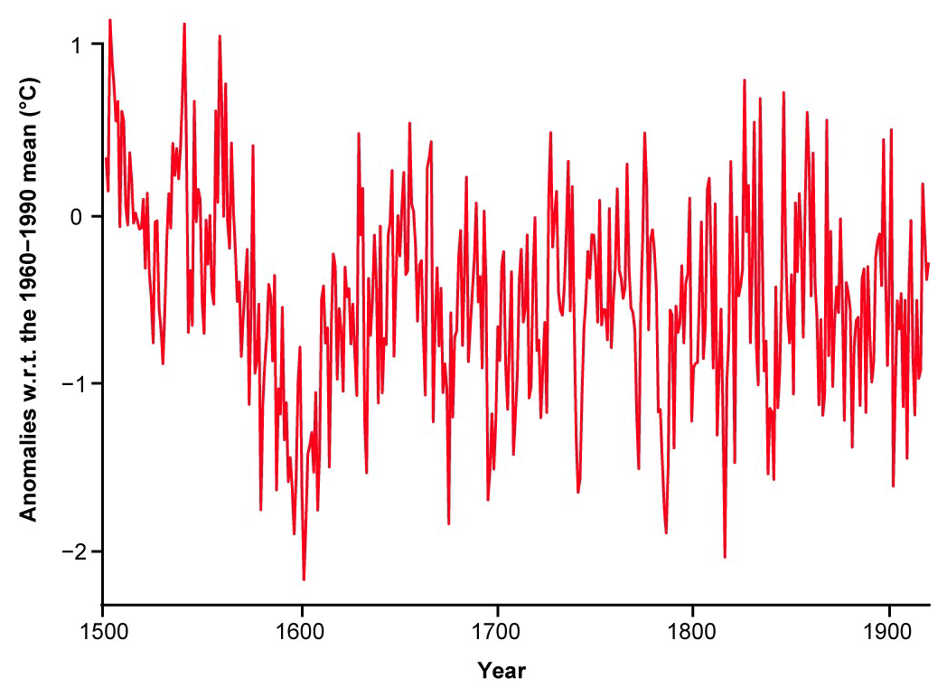
Figure 1The 1500–1920 summer (JJA) temperature reconstruction from Ljungqvist et al. (2019) based on a grid cell at 12.5∘ E and 57.5∘ N, roughly corresponding to Mark Municipality in southern Västra Götaland. Source: Ljungqvist et al. (2019).
During portions of the 18th century, there was a “return” to milder temperatures, albeit with some notable exceptions with especially cold periods in the early 1740s and 1780s. The most notable challenge in terms of natural conditions pointed out in previous research is the increasing degree of sand drift and soil erosion in Scania during the later parts of the 18th century and early 19th century (Mattsson, 1987). As Bohman (2017a, b) has shown, these agro-ecological crises were mostly local and temporary, counteracted by land management policies at the local and regional level. The main causes behind the increasing soil erosion and sand drift have been framed as anthropogenic through deforestation and intensified land use practices. Mattsson (1987), relying on instrumental and observational meteorological records from Lund, argued that another underlying factor behind these agro-ecological issues was climatic variation in the form of the generally colder conditions during the Little Ice Age (LIA) and increased heavy winds and storms, particularly easterlies, during the latter half of the 18th century.
In the following century, the 1810s and the 1840s stand out for being cold (Tidblom, 1876; Cappelen et al., 2019). In general, the 19th century was one of great transformation and expansion for agriculture in Scania, making it difficult to identify any prolonged climatic periods that were beneficial or detrimental for agriculture. Nonetheless, there certainly were years that experienced particularly bad agrometeorological conditions like summer droughts, for example in 1811, 1822, 1826, 1837, 1868, 1870, and 1899 (Tidblom, 1876; SMHI, 2021). The 1868 summer drought was particularly bad since it followed a year of severe crop failures in northern Sweden that had already depleted much of the grain stocks available for aid (Dribe et al., 2015; Västerbro, 2018). According to Utterström (1957) and Edvinsson et al. (2009), lack of precipitation and drought during the summer were the main agrometeorological risks in southern Sweden in the 18th and 19th centuries.
1.2 Farming in Scania
Descriptions of agriculture in Scania during and subsequent to the study period have relied on the ethnographic and geographical categorizations made by Campbell (1928), who outlined three different types of farming districts: the plain, the intermediate (or “brushwood”, sw. risbygd), and the forest districts (Dahl, 1989; Svensson, 2013). Villages in the plain districts generally practiced a three-field farming system and were characterized by their specialization in grain production (Campbell, 1928). In the intermediate districts, villages had a higher share of livestock production and often practiced a one-field farming system (Bohman, 2010). Finally, the forest districts had the most diversified economy with handicrafts and forest-related industries complementing grain and livestock production (Svensson, 2016). Bohman (2010) estimated that during the 18th century and the first half of the 19th century, crop production constituted roughly 90 % of the total production value in the plains district and somewhere around 80 % in the intermediate and forest districts. Controlling for price changes, crop production increased its share of overall production value at least until the 1860s.
Despite the fact that the types of farming districts varied in their respective specializations, practically all farming in Scania was performed in a mixed farming system, wherein livestock husbandry and grain production were integrated and mutually dependent (Bohman, 2010; Myrdal and Morell, 2013). Until the 19th century, most farms in Scania belonged to a village where farming operated under an open-field system (sw. tegskifte) with a mixture of private and communal management. Limited enclosure reforms, storskifte, were introduced starting in 1757, followed by radical enclosure reforms in 1803 (enskifte) and 1827 (laga skifte). These latter reforms involved the breakout of the individual farms from the communal management, effectively privatizing land ownership and management. Implementation of these reforms was gradual and intermittent (Gadd, 2011, 2018). Hence, for large parts of the study period, decision-making regarding grain production was largely mediated through the institutions of the village.
1.3 Grain crops
Rye, barley, and oats dominated the composition of grain production during the study period and had done so since the Viking Age, albeit with much internal variation over time. For example, oats production saw a large increase in its share of overall grain production during an export boom in the 19th century (Welinder, 1998; Bohman, 2010). In the late 19th century and early 20th century, the new so-called improved cultivars (mainly in the form of autumn rye and autumn wheat) increasingly took the place of the most dominant grain crops (Leino, 2017). Given their dominance in a historical perspective, this study will mainly be limited to analyzing the production of barley, rye, and oat varieties. Wheat varieties will also be included in the later study period (1865–1911).
In previous research, the type of farming district and soil types have been seen as the primary factors determining differences in crop composition (Dahl, 1942, 1989). Wheat and barley were more dominant in the arable plain districts. The share of oats was lowest in the forest districts, and the share of rye was roughly the same in the different types of districts. Regarding soil types, Bohman (2010) found that barley and oats (and wheat) were more dominant on high-quality soils and rye was more common on poorer soils and that in relation to animal production. He also argued that vegetable production increased its share throughout the 18th and the first half of the 19th century as a supply-side response to increasing prices. The share of the total value of agricultural production constituted by vegetable products ranged between 61 % and 97 % through the 18th and 19th centuries depending on decade and parish (Bohman, 2010).
1.4 Rye varieties
Leino (2017) has studied some of the historical grain varieties in Sweden. Examples of rye varieties prevalent in Scania were late rye (sw. senråg), St. Laurentius Day rye (sw. larsmässoråg), sand rye (sw. sandråg), and spring rye (sw. vårråg). Swidden rye (svedjeråg) was most likely also grown, especially in the forest districts. Scanian farmers preferred to grow their rye on sandy soils or other well-drained soils (Dahl, 1989; Gustafsson, 2006). Leino (2017) notes that in historical sources, late rye is often characterized as allowing very late sowing, all through December in Scania (in some extreme cases this nominally autumn crop was apparently sown in early spring). According to Leino (2017), this type of late sowing of late rye offered the possibility to incorporate autumn rye into a two- or three-field system without the need for a full year of fallow after the preceding harvest. This somewhat blurred line between spring and autumn rye is consistent with genomic studies of Scandinavian rye landraces (Hagenblad et al., 2012). More detailed sources on sowing dates are difficult to find. By all accounts sowing dates varied locally. In parish descriptions from Malmöhus county in the early 19th century, sowing dates for autumn rye vary from the middle of August until early October, although the most commonly noted sowing period was the latter part of September (Bringéus, 2013). Spring rye appears to have been sown after barley sometime in May, depending on the village. Autumn rye is noted to have been harvested earlier than other crops, although all harvesting of rye is reported in either late July or August.
In a broader context of European rye landraces in the pre-1900 period, Fennoscandian landraces have been found in genomic studies to belong to a particular and separate meta-population of rye landraces, distinct from landraces in continental Europe. Furthermore, even southern Scandinavian rye landraces have been found to have more in common genetically with landraces from northeastern Europe than those from maritime western Europe (Larsson et al., 2019).
1.5 Barley varieties
Southern six-row barley (sw. sydsvenskt sexradskorn) was common in Scania, especially in the forest districts, even in the late 19th century. It was sown late, often well into June, due to its sensitivity to frost and its rapid growth, allowing ripening despite late sowing. Two-row varieties like Scanian two-row barley (sw. skånskt tvåradskorn) were also grown, at least during the 19th century but probably earlier as well. Two-row varieties required more intensive agricultural practices, longer growth periods, and richer soils but offered better resistance to frost and often gave larger yields compared to six-row varieties. In the previously mentioned parish descriptions from the early 19th century, sowing dates for barley range from late April to early June, while harvesting is mostly described as taking place sometime in August (Bringéus, 2013).
Similar to rye, genomic evidence for barley landraces from Scandinavia and southern Scandinavia in particular indicates spatial and temporal consistency from the 17th century up until the late 19th century (Lundström et al., 2018). A distinctive feature of these Scandinavian barley landraces in terms of genetic markers is the prevalence of the nonresponsive ppd-h1 allele, which prolongs the flowering during periods of increasing daylight, prolonging the vegetative state and potentially increasing yields in cooler and wetter conditions (Jones et al., 2012; Aslan et al., 2015). An allele is one of several possible expressions of a given gene. The ppd-h1 allele is the nonresponse expression of the ppd-H1 (Photoperiod-H1) gene (Turner et al., 2005). It has been suggested that selection and maintenance of barley seed with this particular allele were part of a long-term adaptation process by early farmers (Cockram et al., 2007).
1.6 Oat varieties
Historical oat varieties can be grouped into two broad categories: white oats and black oats. Generally, white oat varieties were grown on poorer, and especially wet, soils. According to Campbell (1950), they were better suited for making bread compared to the fodder-oriented varieties that became increasingly more common during the course of the 19th century. Black oat varieties were more resistant to droughts and were preferably grown on richer, manured soils. Campbell (1950) argued that Nordic white oats (sw. nordisk vithavre) were the most common variant in Scania. It is more uncertain whether black oat varieties were grown, although they were grown in all neighboring provinces (Halland, Blekinge, and Småland), which suggests, together with the fact that there was a widespread trade in seed grains, that black oats were at least grown locally and intermittently (Campbell, 1950; Leino, 2017). Oats appear to have been sown about 1–3 weeks prior to barley and spring rye and harvested at about the same time as, or shortly before, barley (Bringéus, 2013).
According to Dahl (1942), oat farming in Scania was not an adaptation to local climate like in parts of northwestern Europe. Rather, it was other natural conditions, primarily the type of moraine soil common in some areas around the Baltic like Denmark, Scania, and northern Germany (sw. baltisk morän), as well as local hydrological conditions, namely on soils that were poorly drained, that were decisive for oat cultivation. It is important to note that Dahl (1942) conceptualized natural conditions and climate as something static and that the only secular changes that occurred in natural conditions were due to human intervention, for example by not investing in drainage or through over-cropping. However, given that the climate actually varied over time, one would expect climate effects interacting with factors like soil and the type of cultivated crop. For example, periods of a wetter climate should have had more negative impacts on crops grown on poorly drained soils, whereas crops cultivated on well-drained soils should have been more exposed to drought periods (Osvald, 1959; Weil and Brady, 2017).
This brief overview of the diversity of grain varieties to be found in early modern Scania suggests a flexible farming system in terms of sowing and harvest dates as well as the ability to produce grains under differing agrometeorological conditions. It is important to note in this context the inherent capacity of crop varieties to adapt to local environmental conditions (including local farming practices) that over time should have led to much greater variety, and indeed resilience, than this brief overview suggests (Leino, 2017; Aslan et al., 2015). In the context of historical grain production, I define resilience as the ability of a production system to maintain itself over a longer period through a combination of biological and institutional flexibility and durability in the face of a variable environment. When discussing adaptation I refer to how a given crop or farming practice performs in a given set of environmental circumstances. I subsume the concept of exaptation (passive or accidental adaptation) under adaptation, given the difficulty in disentangling the two. For example, a particular crop may perform better during colder periods, increasing the production of the crop, which could be due to farmers actively adapting to changeable circumstances or the crop being more adapted (passively) relative to the other crops being cultivated. Moreover, even if farmers are actively increasing the production of a given crop, it can still be very difficult to establish whether it is due to adaptation to environmental change, a response to shifting market demands, technological innovation, or cultural trends.
Previous research has stressed that, at least in relation to climate “extremes”, diversified crop production including both spring and autumn crops of different varieties was more resilient in areas of Europe north of the Alps (Michaelowa, 2001; Ljungqvist et al., 2021a). Michaelowa (2001) partly blamed the excess specialization towards autumn wheat for the relatively poor performance of French agriculture compared to English agriculture during the 18th century; the latter was more diversified, cultivating autumn wheat, autumn rye, and spring barley and oats.
Utterström (1955) and Michaelowa (2001) argued that colder periods in the early modern period, specifically in the late 17th and 18th centuries, led to reductions in livestock production in France, England, and Sweden, and in response grain production usually increased with the intention to fill in the nutritive gap. If such adaptations took place, they must have been difficult to implement in the short term and were probably also insufficient given that grain production was also vulnerable to spats of cold weather. Pfister (2005) showed how cold and wet conditions during the different seasons of the year were detrimental to livestock production in the Swiss Alps as well as the difficulties of the local communities to adapt given that the cultivated grains and vines were also vulnerable to cold and wet conditions. Grain shortages, sometimes resulting in famines, were common in many parts of Europe up until at least the 19th century (Appleby, 1980; Dribe et al., 2015; Esper et al., 2017).
There have been attempts to detail the relationship between grain production and climate variability in northern Europe during the early modern period in more detail. Brunt (2004) found that English wheat yields during the 1770s were mainly sensitive to temperature and to a lesser extent precipitation, depending on local soil conditions. Especially important were summer temperatures. Cooler summer temperatures through the month of July benefited wheat yields, supposedly by prolonging the grain-filling period. A warm and dry August was then beneficial by allowing the crops to dry for the coming harvest. Ideally, rainfall would be spread out over many days during the early summer months. Concentrated rainfall during a short time span risked ruining the crop, with the harvest month of August being especially vulnerable (Brunt, 2004). In a later study, Brunt (2015) found that wheat yields were significantly affected by weather shocks throughout the ca. 1690–1850 period (to the extent that they obfuscated subsequent estimations of long-term productivity trends), with the 19th century largely conforming to the 1770s as to the effects from temperature and precipitation during summers.
Pei et al. (2016) studied the relationship between yield ratios and temperature at a continental scale and proposed that European farmers during the period ca. 1500–1800 used crop management as a mechanism for climate adaptation. Specifically, farming systems drifted towards increased rye production during colder periods, which the authors argue was a more cold-resistant crop. In an earlier study, Pei et al. (2015) asserted that extensification of land use was the most prominent strategy in mitigating climatic stress during the same period. However, given differences in soil, climate, available grain varieties, and other factors, it seems more reasonable to expect more heterogeneous and contextually dependent adaptation practices at the local and regional level (van Bavel et al., 2019; Ljungqvist et al., 2021a). While rye was almost certainly more cold-resistant than wheat, in relation to oats the same seems to be true only when we exclude wetter climatic areas (e.g., western Sweden or parts of Scotland). In relation to barley there is limited evidence indicating that rye was the more cold-resistant grain overall. For example, in northernmost Sweden and Finland grain production was limited almost exclusively to barley. An important caveat in making these types of comparisons is the fact that rye was mostly grown as an autumn crop, whereas barley and oats were exclusively grown as spring crops and that in many agricultural areas of northern Europe they were more often supplementary than rival crops (Huhtamaa and Helama, 2017b).
Considering Sweden, and southern Sweden in particular, one finds a composition of grain production that was diversified and comparable to that of England in the 18th century described by Michaelowa (2001), with the important exception of wheat, which in Sweden was only a marginal crop. Utterström (1957) argued that for grain production in northern Sweden, temperature was the most important climatic variable, whereas it was precipitation for southern Sweden. Using more up-to-date climate and grain harvest data, Edvinsson et al. (2009) largely confirmed the stipulations made by Utterström (1957), at least from 1724 up until the late 19th century, finding a negative association between subjective harvest assessments and June and July temperatures and a positive association with precipitation in the same months and November and December temperatures. After ca. 1870, Edvinsson et al. (2009) found a shift in the relationship. Precipitation in the summer, including the month of May, was still positively correlated with the harvest assessments. However, summer temperatures were no longer statistically significant, whereas the first 4 months of the year (JFMA) showed positive associations with harvests assessments. A short digression is in order here. Compared to summer and spring temperatures, relationships with winter temperatures are more difficult to explain, given that they are indirect, occurring before the growing season for spring crops. Temperature and precipitation during the winter months do affect the overwintering autumn crops by facilitating or inhibiting the survival of the grains themselves, as well as fungi, soil bacteria, and other various grain pests (Holopainen and Helama, 2009; Osvald, 1959). In addition, the nutritive balance of the soil is affected (Ađalsteinsson and Jensén, 1990). Again, it is quite difficult to establish, both empirically and theoretically, the mechanisms and links between these relationships and the subsequent grain harvest. It should be noted that these “indirect” effects are also at play during the other seasons. For example, de Vries et al. (2018) found that summer droughts have different effects on soil bacteria and fungus and that these effects have long-term consequences for vegetation growing on the soil.
Returning to the discussion of the results from Edvinsson et al. (2009), they argued that the overall relationship between climate variability and grain harvests was weak, partly explained by the lack of detail in climate data. Furthermore, they found that the magnitude of the relationships increased in the period 1871–1955 compared to the previous roughly 150 years, which they primarily explained in terms of the increasing shift towards higher-yielding and more temperature-sensitive wheat production. More controversially, they also hypothesized that climate variability itself was less important to harvest in pre-industrial agriculture due to chronic seed shortages and more risk-averse behavior on the part of farmers.
With respect to the differences between different grains, Edvinsson et al. (2009) employed aggregate official statistics at a national level for the period 1803–1955 (with a gap between the years 1821 and 1859). They found that wheat and rye harvests were positively correlated with October through April temperatures, that barley harvests were positively correlated with temperatures in April, May, and August–September, and finally that oat harvests were negatively correlated with June–July temperatures. Harvests of all the mentioned grains were positively associated with increased precipitation in May through July. Wheat and rye harvests were negatively associated with increased precipitation in March, whereas the same was true for barley and oat harvests in relation to precipitation in September. These results are possibly skewed towards the late 19th century and especially the first half of the 20th century considering the gap between 1821 and 1859 as well as the dramatic shifts in the types of cultivated grain varieties that Sweden underwent in the late 19th century (Leino, 2017). Beside the study from Edvinsson et al. (2009), Palm (1997) tried to estimate the relationship between the yields of various grains at a farm in Halland between ca. 1750 and 1870, with limited results.
The division of Sweden into a southern and northern half in regards to the main agrometeorological constraints for agriculture and grain production made by Utterström (1957) and later affirmed by Edvinsson et al. (2009) arguably needs to be complemented. As discussed by Huhtamaa and Ljungqvist (2021), the relationships between climate and agriculture in Scandinavia vary from region to region. From an agronomic perspective, southern Sweden is a diverse place in terms of natural geography. Northwestern Scania and the provinces further north on the west coast (Bohuslän, Halland, Västra Götaland) are wetter and colder than most of Scania, whereas most of the east coast of southern Sweden is drier (especially during spring and autumn) and experiences on average a few hundred extra hours of sun each year (Persson et al., 2012). As mentioned previously, Scania stands out relative to the rest of southern Sweden in terms of the duration of the growing season (Osvald, 1959). Huhtamaa and Ljungqvist (2021) propose that in neighboring Denmark hosting similar conditions for grain production, the shortening of the growing season during wetter and/or colder years might not have led to major issues related to frost. Important additions to these considerations of natural geography include the question of what types of grain varieties were cultivated and in what type of farming system.
In the following sections, I attempt to estimate the relationship between climate variability and grain production in Scania during the period 1702–1911, divided into an early study period (1702–1865) and a later study period (1865–1911). First, I describe and discuss the sources and methods employed, followed by a presentation and a discussion of the results. Finally, I conclude the article by interpreting and contextualizing the obtained results.
3.1 Sources on agriculture and grain production
Scania stands out in the Swedish context regarding the availability and extent of specific historical source material, namely the priestly tithes (sw. prästetionde), which in many parts of Scania remained flexible and proportional to output throughout the 18th and 19th centuries (Olsson and Svensson, 2010). Using surviving tithe records from 36 parishes in Scania, Olsson and Svensson have produced a database, the Historical Database of Scanian Agriculture (HDSA), with roughly 85 000 unique farm-level observations covering the period 1702–1881, wherein one observation is one farm's production in 1 year (Olsson and Svensson, 2017b). The structure of the HDSA is that of an unbalanced panel and includes, besides production data on crops and animals, data on farm size and household characteristics, land tenure and other institutional factors, soil quality and land size, geographical factors, and relative crop and animal prices.
The soil data in the HDSA are based on modern soil grading. Previous historical studies have relied on modern soil grading, arguing that it better captures the “natural” fertility of agricultural landscapes compared to those found in historical sources. For instance, Brunt (2004) used national survey data from the 1950s and 1960s in his study of historical grain production in England. The English national soil survey was predominantly based on geological and climatological indicators (Gilg, 1975). Bohman (2010) used data from Göransson (1972), who performed a local study of soils in Scania based on the gradient system established by the Swedish national soil survey published in 1971, which was based on a mix of geological, yield, and price data as well as local expertise (Lantbruksstyrelsen, 1971). The data from Göransson (1972) have subsequently been incorporated into the HDSA. The soil grading system was based on 10 levels; 1 denotes the lowest and 10 the highest-quality soils. According to the national survey, Scania was the only region in Sweden with grade 10 soils (Lantbruksstyrelsen, 1971).
Constructing grain production series for the earlier period 1702–1865 from the HDSA involves attempting to solve some issues. Firstly, there is an issue related to how the tithe was collected, i.e., that it was collected before threshing, and the amount of seed that was obtained by threshing the same type of grain differed across parishes and farming districts. Therefore, all crop production series are adjusted to local threshing coefficients based on actual threshing accounts in different parishes, in line with Olsson and Svensson (2017a).
Secondly, there are issues of nonstationarity in grain production time series, particularly in the 18th century and beyond, requiring detrending methods in order to obtain reliable and linear estimations of relationships (Jörberg, 1972; Huhtamaa, 2015; Shumway and Stoffer, 2017). At the same time, detrending risks removing information related to the long-term effects of climate variability on grain production (see Esper et al., 2017, and Ljungqvist et al., 2021b, for a discussion of this in the context of historical grain prices). I estimate normalized production anomalies (NPAs) in line with Beillouin et al. (2020) by employing a locally weighted scatterplot smoothing (loess) for each grain as well as total grain production in the HDSA. Beillouin et al. (2020) used the term normalized yield anomalies, but given that this study mainly relies on production or harvest data, the term yield has been substituted with the term production to avoid confusion (since, for example, sowing intensity per area unit can vary, it is often important to distinguish the harvest from yield in general when discussing agricultural production). A common smoothing span of 0.25 is used for all series. The formula for the NPA is
where is the normalized production anomaly for a given grain in a cluster or aggregate region at each t year. Yt is the average of the observed annual production outcome for the specific grain. μt is the expected production outcome according to the loess fit.
Thirdly, there is the issue that the HDSA panel is unbalanced. Similar to, for example, tree-ring-based temperature reconstructions, with the number of tree rings available for the reconstruction usually declining further back in time (Esper et al., 2016), the number of farms in the HDSA is lower in the early decades of the 18th century (the number of farms also goes down in the final decades of the database coverage). This introduces an increased risk of sampling bias. This problem is partly counteracted by the loess detrending and partly by clustering the data into most similar clusters using hierarchical cluster analysis, as described in Sect. 2.2.
Grain production data are only available up until 1865 in the HDSA. After 1865 there are instead official statistics on grain production on the county and parish levels based on reports from the local rural societies (sw. Hushållningssällskapen) up until 1911, henceforth referred to as the BiSOS data (SCB, 2021). I rely on county-level data only. The 19th century Swedish official statistics have been subject to some important criticisms. The manner in which the data were collected varied to some extent locally as it was up to the local representatives in the rural societies to establish data collection procedures (Svensson, 1965). This is less of an issue considering that I do not compare different parishes with the BiSOS data. Moreover, it is commonly argued that total crop production and the amount of arable area are systematically underreported and underestimated in the official statistics. Again, this is not an issue to the extent that I am principally interested in the variations in output over time that are associated with climate variability. There are no obvious reasons to suspect that this part of the variation in output is related to the general underestimation in official statistics. BiSOS data are detrended by applying the same technique as for the HDSA, namely with estimations of NPA (see Eq. 1).
3.2 Clustering
Considering the institutional and geographical diversity of Scania, aggregating the data risks masking location- or type-specific relationships between agriculture and climate or, conversely, some localized trends distorting the overall picture. To homogenize data from the HDSA, obtain clearer signals, and reduce the risk of introducing a geographical or institutional bias by grouping the data by parish, type of farming district, or cadastral status, all villages in the sample are divided into three different clusters using a hierarchical cluster analysis (HCA).
HCA is an algorithmic-based method that clusters the data into “most similar” groups based on a chosen parameter in the data, in this case threshing-adjusted rye production over time on the village level (see Sect. 2.1). Rye was one of the two most important grains during the study period, and since it was mainly grown as an autumn crop it required some specific management practices at the village level and therefore serves as a more appropriate distinguisher than barley or oats. I use an agglomerative HCA, whereby each village initially forms a cluster by itself, pairing up with other villages as the hierarchy “moves up” (Day and Edelsbrunner, 1984). Distances between groups are estimated using the Ward's D method and Euclidean distances. Euclidean distance is the straight line between two points in classical metric space (Howard, 1994). In HCA the true or optimal number of clusters is not known and the number of clusters is therefore determined by some metric or criteria determined by the researcher. Multiple such criteria have been suggested in the literature, often relating to the largest visible or measurable distances between the branches in the cluster dendrogram. One of the most common such metrics is the gap statistic (Tibshirani et al., 2001). Specifically, I use the clusGap function in the factoextra package in R, setting the maximum number of potential clusters at 10 and running 100 bootstrap samples (Kassambra and Mundt, 2020).
Some descriptive and interpretative issues come with this approach. If a resulting cluster consists of several different types of farming districts and administrative units, e.g., parishes, separated into different clusters, then describing, interpreting, and contextualizing results become difficult. In order to reduce the descriptive and interpretative issues related to the HCA, the clustering results thus obtained are contextualized using the most common historical categorizations found in the historical literature when discussing regional specialization in agricultural production, namely the type of farming district (see Sect. 1.3). Clusters are also described in terms of cadastral status and soil characteristics using information available in the HDSA.
3.3 Grain production clusters
Figure 2 shows the cluster dendrogram obtained using the method described in Sect. 2.2, cut at three clusters. Describing these clusters in terms of historical and geographical categorizations, some distinguishing patterns emerge.
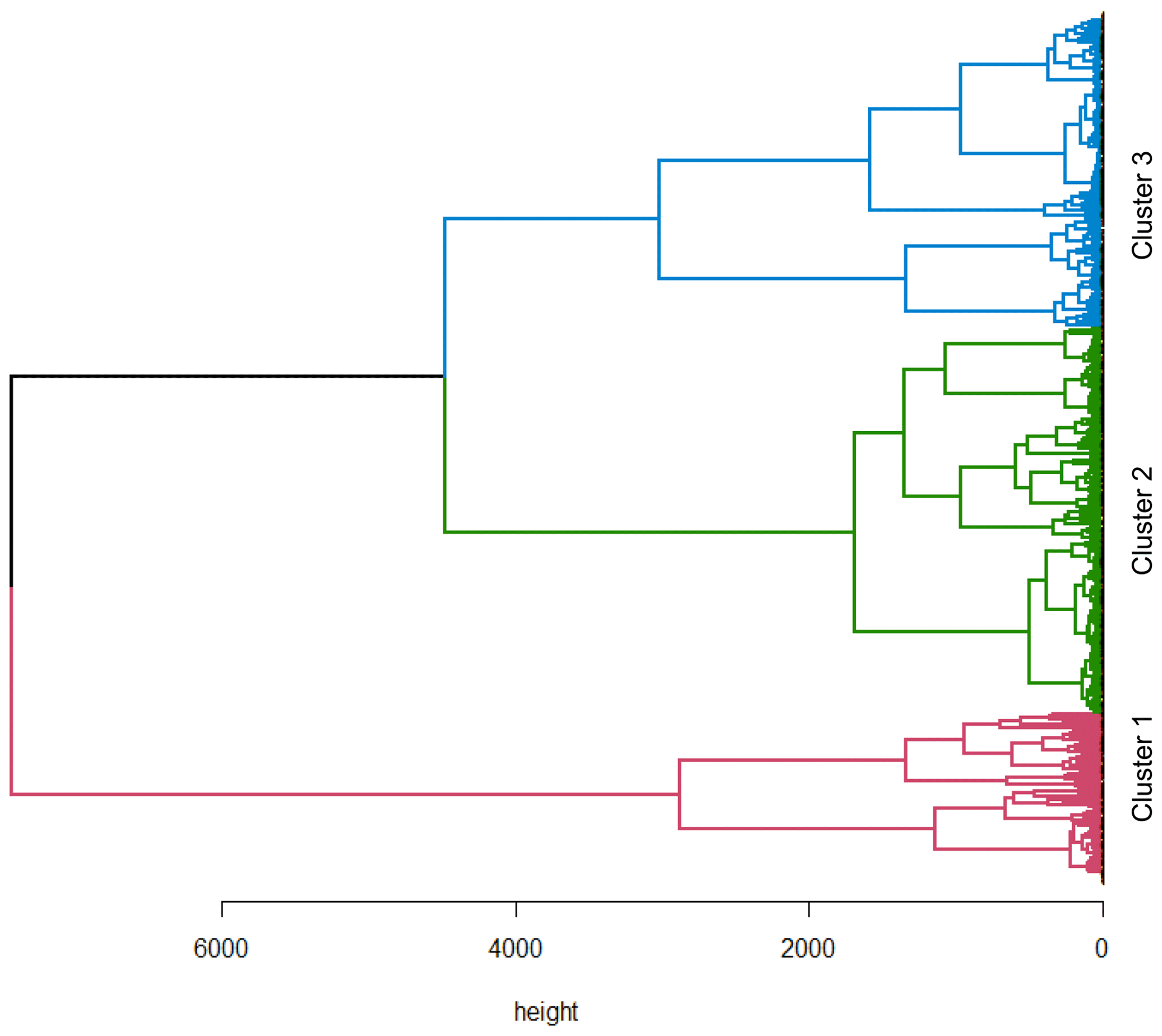
Figure 2Cluster dendrogram illustrating the sorting process leading to three most similar clusters. Source: HDSA.
Figure 3 reveals that all clusters are represented by villages in the northernmost parishes of Hjärnarp and Tostarp, the forest and mixed farming districts centered around Billinge and Kågeröd parishes, and the parishes located in the forest and mixed farming districts around lake Vomb in southern Scania. Cluster 1 is most heavily represented by the parishes in the proximity of Billinge and Kågeröd as well as around lake Vomb. Cluster 2 is the most geographically spread, covering all of the areas of the total sample, except the plain district parishes around Malmö and Lund. Finally, cluster 3 is mostly concentrated on the parishes around Malmö and Lund, with some villages in parishes around Röstånga and Kågeröd as well as around the southern edges of lake Vomb.
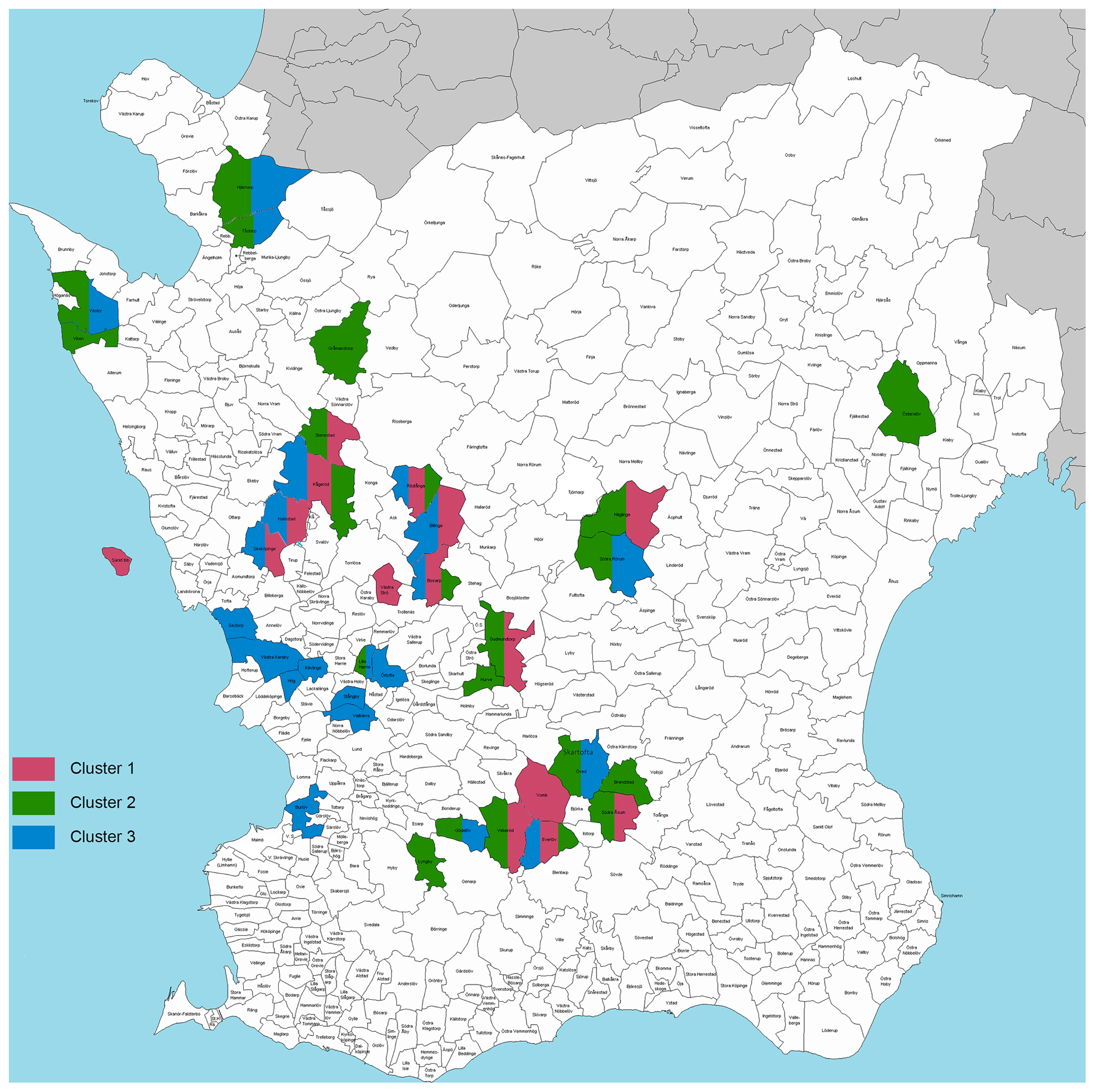
Figure 3Geographical and administrative (parish) representation of each cluster. Source: author's own edit of the parish map of Scania from Wikimedia Commons (Mrkommun, 2010).
Table 1 shows the outcome from the clustering in terms of proportion of arable land in each grade. Cluster 1 has the largest share of the low-quality soils (grade 1 to 4) of roughly 39 %, as well as the least amount of high and moderately high-quality soils (grade 7–8 and 9–10). Cluster 2 has the largest variance in terms of shares in different types of soils as well as the largest share of moderately high-quality soils of ca. 54 %. Finally, cluster 3 has the largest share of the highest-quality soils at 16 %, as well as the largest amount of moderate soils at 44 %.
Table 1Descriptive statistics for each cluster, including proportions of soils of different qualities.
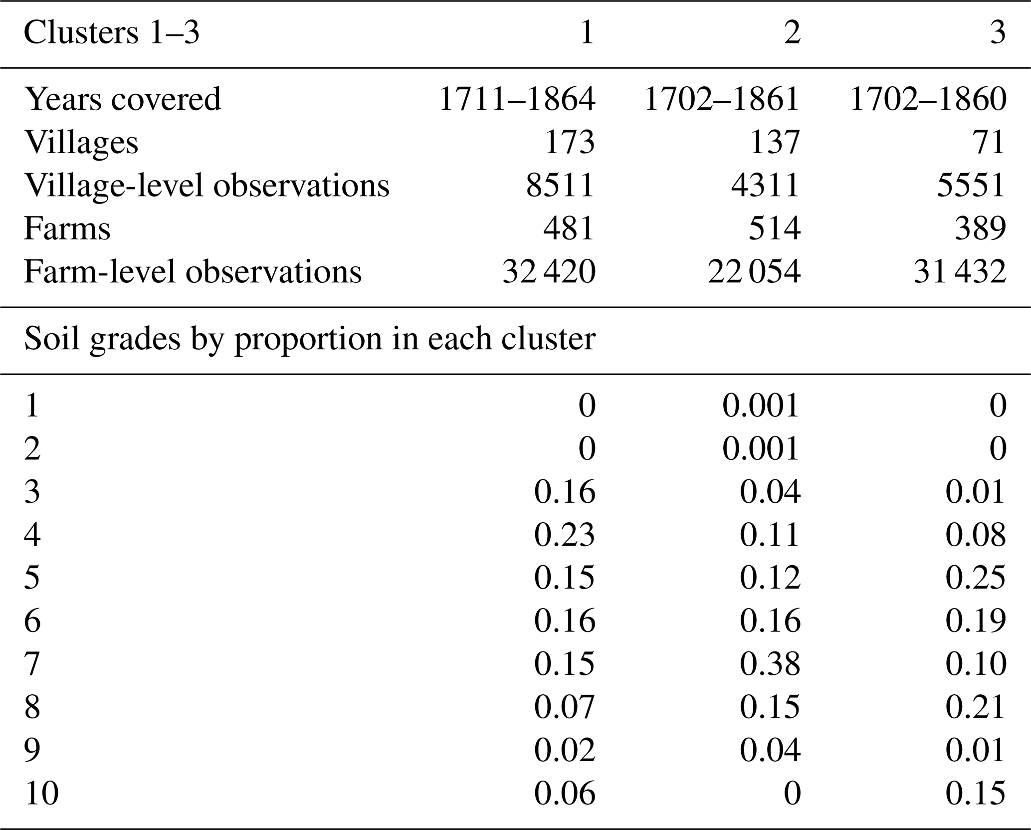
Note that there are no grade 1–2 soils in the sample, whereas the amount of the highest-grade (8–10) soils is quite large. Source: HDSA.
Figure 4 below shows the number of villages from each type of farming district in the three clusters as well as the institutional make-up in terms of property rights regimes of each cluster (i.e., freehold land owned and managed by peasant farmers, crown land owned by the state but managed by tenants, and manorial land owned by the nobility but managed by their tenants). Cluster 1 is more mixed, with farms in all three different types of farming districts, albeit with most farms in the intermediate and forest districts, with a moderate share of peasant-owned and managed farms. Cluster 2 has the largest number of manorial farms and almost all farms are located in the intermediate and forest districts. The largest number of plain district farms can be found in cluster 3, which also has the largest number of crown and peasant-owned farms. Furthermore, cluster 3 contains almost no intermediate district farms and a moderate number of farms in the forest districts.

Figure 4Institutional status of farms, including type of farming district. Each bar plot represents a cluster with each cluster denoted in the grey-marked area. 1 denotes plain districts, 2 mixed districts, and 3 forest districts. Source: HDSA.
In terms of grain production, cluster 3 has the largest average production of all grains over time as well as the largest share of rye and barley in its production, which is not surprising given that it has the largest share of plain district villages as well as the largest share of the highest-quality soils, as shown in Fig. 5. Cluster 2 has similar average production levels as cluster 3 in the first decades of the 18th century, followed by a slight stagnation for the rest of the century, then by large increases in production of all grains, in particular oats, during the first half of the 19th century. The cluster with the lowest-quality soils, cluster 1, also has the lowest average production levels, although it shows continual increases throughout the period 1702–1865.

Figure 5Average grain production (threshed hectoliters) in each cluster over time, including estimated loess. For cluster 1 the years 1743–1746 are covered by only one farm, heavily skewing the average for those years. Therefore, I have substituted the values for rye and barley for the years 1743–1746 with values obtained from a linear estimation of the relationship between the production of that farm and the average production in the cluster in the years 1727–1742. Source: HDSA.
To summarize, cluster 1 is institutionally mixed and has the lowest-quality soils; cluster 2 is more manorial, has the largest share of soil grades 6–10 of all the clusters, and is the most geographically spread cluster. Finally, cluster 3 is mostly peasant-owned or managed and has the largest share of the highest-quality soils (grade 8–10) and lands in the plain districts, notably in the plains around Lund. Average production levels increase in ascending order from cluster 1 (the lowest) to cluster 3 (the highest), although there is some variation over time.
3.4 Sources on the climate
Temperature is one of the most important agrometeorological indicators, especially during the growing season. Instrumental temperature measurement data are available from the city of Lund from the year 1753. The series contains gaps and has several noted inhomogeneities in the form of instrument relocations, instrument replacements, and changes in observers (Tidblom, 1876). For the purposes of this study, the temperature series was homogenized and gaps were filled using adapted Caussinus–Mestre algorithm (ACMANT) software relying on the target unhomogenized temperature series as well as a network of homogenized temperature series (Domonokos and Coll, 2017). The homogenization procedure is further detailed in Appendix A. Results of the homogenization procedure are also presented and discussed in Sect. 3.2 and 3.4. I use a homogenized monthly temperature time series centered on Lund from 1702–1865, including infilling of gaps between 1702–1752 and 1820–1833.
I also use precipitation data from Lund, available from 1748, as well as the number of rainy days per month (Tidblom, 1876). Hydroclimate is much less spatially coherent compared to temperature; hence, a similar homogenization approach in line with the temperature series is not suitable. Therefore, I supplement the instrumental precipitation data with regional hydroclimate reconstructions. I use three hydroclimate reconstructions. The first, from Cook et al. (2015), is a Palmer Drought Severity Index (henceforth, PDSI) reconstruction from the Old World Drought Atlas, covering the entire study period; I use the grid cell centered at 55.75∘ N, 13.75∘ E, roughly corresponding to east-central Scania. The second is a reconstructed standardized precipitation–evapotranspiration index (henceforth, SPEI) for southern Scandinavia compiled by Seftigen et al. (2017), which also covers the whole study period (see Fig. 6). These two reconstructions are independent and based on mutually exclusive data. The third and final hydroclimate reconstruction is a May through July precipitation reconstruction (henceforth, MJJpr) by Seftigen et al. (2020) based on the wood densitometric indicator referred to as blue intensity (BI), covering the period after 1798. The second and third reconstructions are not strictly independent given that they are based on the same tree-ring data, although they are extracted using different methods and the MJJpr is more oriented towards capturing high-frequency variability (Seftigen et al., 2020).
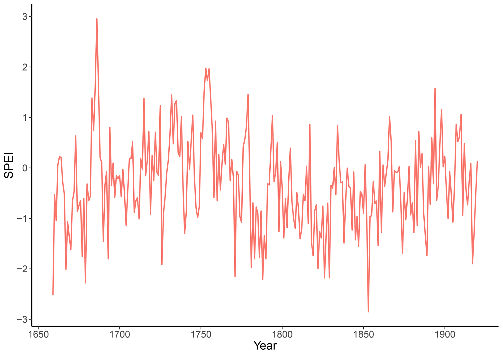
Figure 6Reconstruction of southern Scandinavian SPEI, 1659–1920. Source: Seftigen et al. (2017).
For the period after 1865, I use monthly average, minimum, and maximum temperatures and monthly accumulated precipitation instrumental data, also from Lund, available at the Swedish Meteorology and Hydrology Institute (SMHI, 2021), as well as the hydroclimate reconstructions mentioned above. I also use daily air temperature data from Lund during the period 1863–1911 to calculate the average occurrence of the first autumn frost and last spring frost. Given that ground temperature can vary from air temperature, I use a slightly conservative estimate; days with 1 ∘C or less in average temperature between January and May are considered days with spring frosts and between June and December are autumn frosts. These estimates are then compared to estimations made by SMHI for the period 1960–1990.
Some studies employ climate variables based on annual change, month-to-month changes, or anomalies from some long-term or moving trend when estimating the relationship between historical grain production and climate (Brunt, 2004; Edvinsson et al., 2019; Bekar, 2019). However, the evidence of any potential information added by increasing the complexity of the climate variable involved has been limited (E. Vogel et al., 2009; M. M. Vogel et al., 2019). Thus, I follow the example of Beillouin et al. (2020) and use “simple” climate variables.
3.5 Estimating the relationship between grain production and climate
The main analysis is based on cluster-wise Pearson correlation analysis of pairs of variables. I estimate correlation coefficients between annual normalized yield anomalies of rye, barley, oats, total grain production, and climatic variables on a monthly and seasonal basis using HDSA for the early study period 1702–1865 and the BiSOS data for the later period 1865–1911. Given that harvesting was usually completed in late August or during September, I have used lagged (i.e., the values from the previous year) climatic variables for the autumn and early winter months (OND). In addition, I estimate the same relationships during drier and wetter years, respectively. Wet and dry years for the HDSA are defined according to the 33rd (dry) and 67th (wet) percentiles of the SPEI during the period 1651–1951. For the HDSA period, this translates to 58 dry years and 55 wet years (see Tables B1 and B2 in Appendix B). Due to the low n in the latter period 1865–1911 (n=47), I split the data into two halves, each representing the lower (drier, n=23) and higher (wetter, n=24) halves of the SPEI during those years (see Tables B3 and B4 in Appendix B).
4.1 Estimations of past temperatures and frequencies of growing season frosts in Scania
In this section, I present the results from the estimations of two agrometeorological indicators, both specifically related to temperature. First, I present the main results from the monthly temperature series homogenization for the early study period. Second, I describe the results regarding the average occurrence of the first autumn frosts and last spring frosts during the late study period.
4.1.1 Monthly temperature series homogenization
After homogenization of the Lund monthly temperature series, the largest corrections occur during the summer (JJA) and autumn (SON) months, with temperatures adjusted upwards, especially during the late 18th century (see Figs. 7 and 8). There is a slight tendency for upwards adjustments for the spring (MAM) and winter (DJF) temperatures as well, although it is comparably small. Several breaks were detected in the temperature series, almost exclusively at points in time when there was a change in observer and change in observation location (see Appendix A). The largest breaks occurred in the late 18th century, and smaller inhomogeneities were detected throughout the early instrumental period, except for the 2 earliest decades, 1753–1774, when no significant breaks were detected. The homogenization process is discussed in more detail in Appendix A.
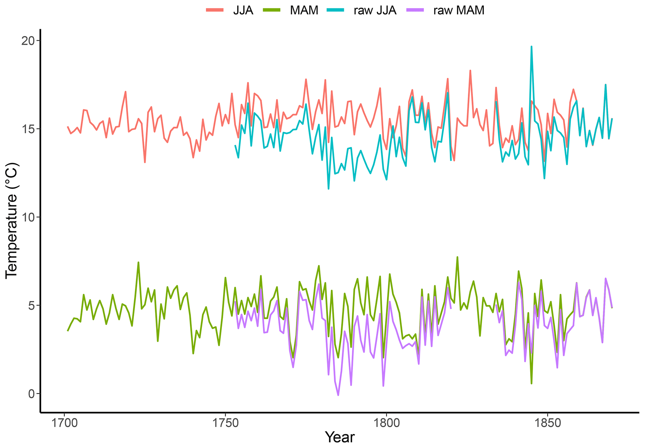
Figure 7Raw and homogenized seasonal JJA and MAM mean temperatures at Lund, 1701–1870. Sources: Copenhagen (Cappelen et al., 2019), Berlin–Dahlem (DWD, 2018), De Bilt (Durre et al., 2008; Lawrimore et al., 2011), Lund (Tidblom, 1876), Uppsala (Bergström and Moberg, 2002), and Stockholm (Moberg et al., 2002; Moberg, 2021). Note: see Appendix A for a further discussion of the homogenization process.
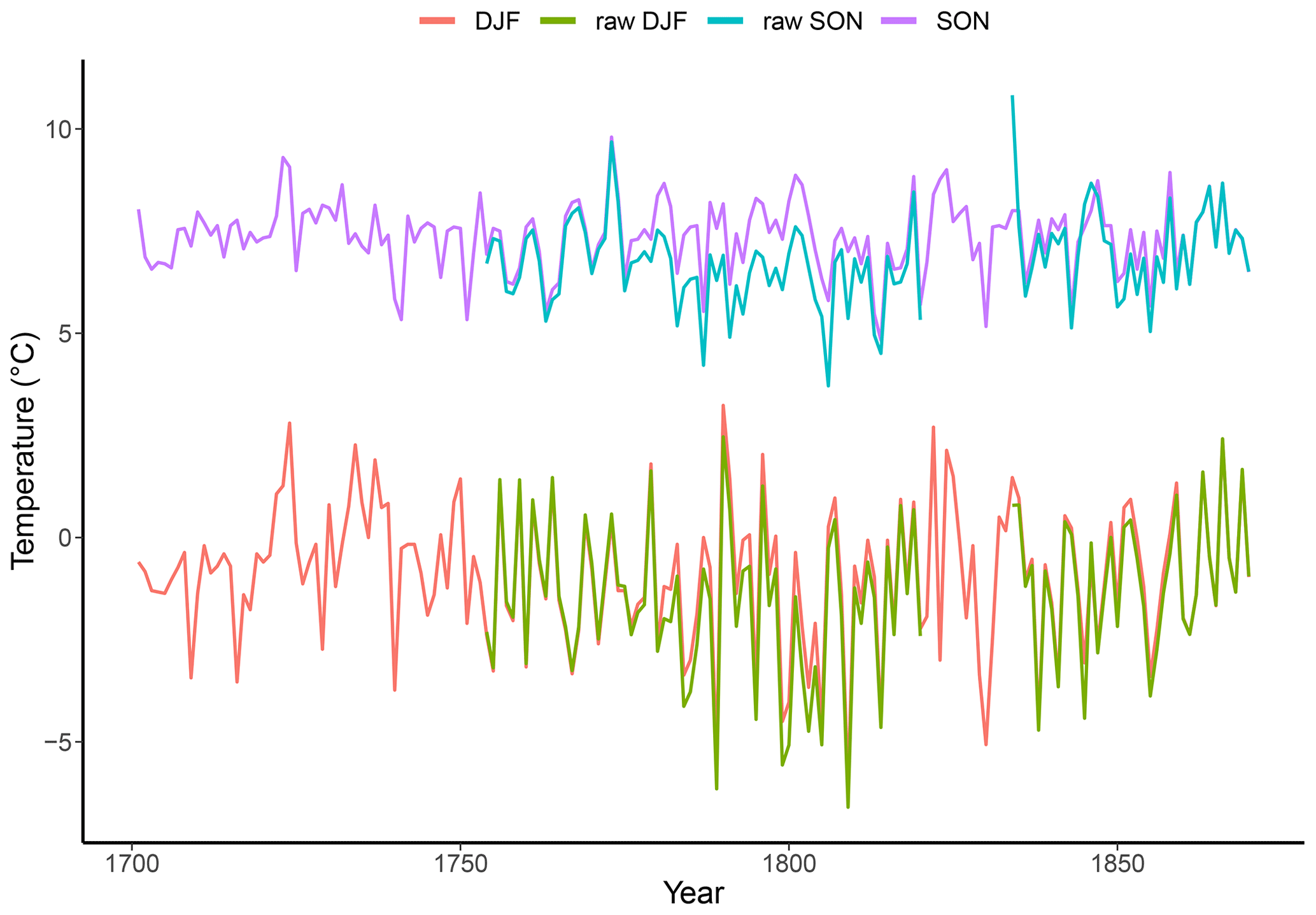
Figure 8Raw and homogenized seasonal DJF and SON mean temperatures at Lund, 1701–1870. Sources: Copenhagen (Cappelen et al., 2019), Berlin–Dahlem (DWD, 2018), De Bilt (Durre et al., 2008; Lawrimore et al., 2011), Lund (Tidblom, 1876), Uppsala (Bergström and Moberg, 2002), and Stockholm (Moberg et al., 2002; Moberg, 2021). Note: see Appendix A for a further discussion of the homogenization process.
4.1.2 Average occurrence of the first autumn frost and last spring frost, 1863–1911
The average date for the last spring frost during the 1863–1911 period was 15 April. In almost half (44 %) of these years, there were no occurrences of temperature measurements below 1 ∘C. Only 2 years experienced late spring frosts in May, namely the years 1864 and 1867, in which the latest estimated spring frost was 24 May in 1867, a year which is known for its exceptionally cold spring (Västerbro, 2018). The average date for the first autumn frost was 8 November. The earliest estimated autumn frost occurred on 16 October 1879. These dates are similar to those estimated by SMHI using data from the 1960–1990 period, for which the average date for the first spring frost was between 1 and 15 April in the western and southwestern edges of Scania, between 15 April and 1 May for the rest of western and southern Scania, and finally between 1 and 15 May in northern and northeastern Scania (SMHI, 2017a). The average date for the first occurrence of autumn frosts follow a similar geographical pattern, e.g., between 15 November and 1 December for the western edges of Scania to between 1 and 15 October for the northernmost forested areas bordering Småland (SMHI, 2017b).
4.2 Relationship between climate variability and grain production
In this section, I present the correlation results between climate and grain production indicators in the early and late study periods, respectively. Furthermore, I present correlation results of restricted samples with years including dry or wet summers analyzed separately.
4.2.1 Grain production and climate variability 1702–1865
During the bulk of the period of 1702–1865, there is a negative association between summer temperatures and grain production in all three clusters, with July and June producing the strongest signal, as shown in Fig. 9. May yields low negative correlation coefficients for rye in clusters 1 and 3, and August yields a low negative coefficient for barley in cluster 1. Overall, the signal obtained from the oats series is weak and mostly divergent from the other grains, except for its strong positive association with a higher SPEI, i.e., wetter summer conditions, which it has in common with the other grains. The seasonal temperature indicators largely correspond to monthly indicators, with JJA consistently showing strong negative associations with total grain production in all clusters. Except a low positive association between oat production and spring temperatures in cluster 3, monthly and seasonal temperature indicators for the spring and autumn give almost no statistically significant results.
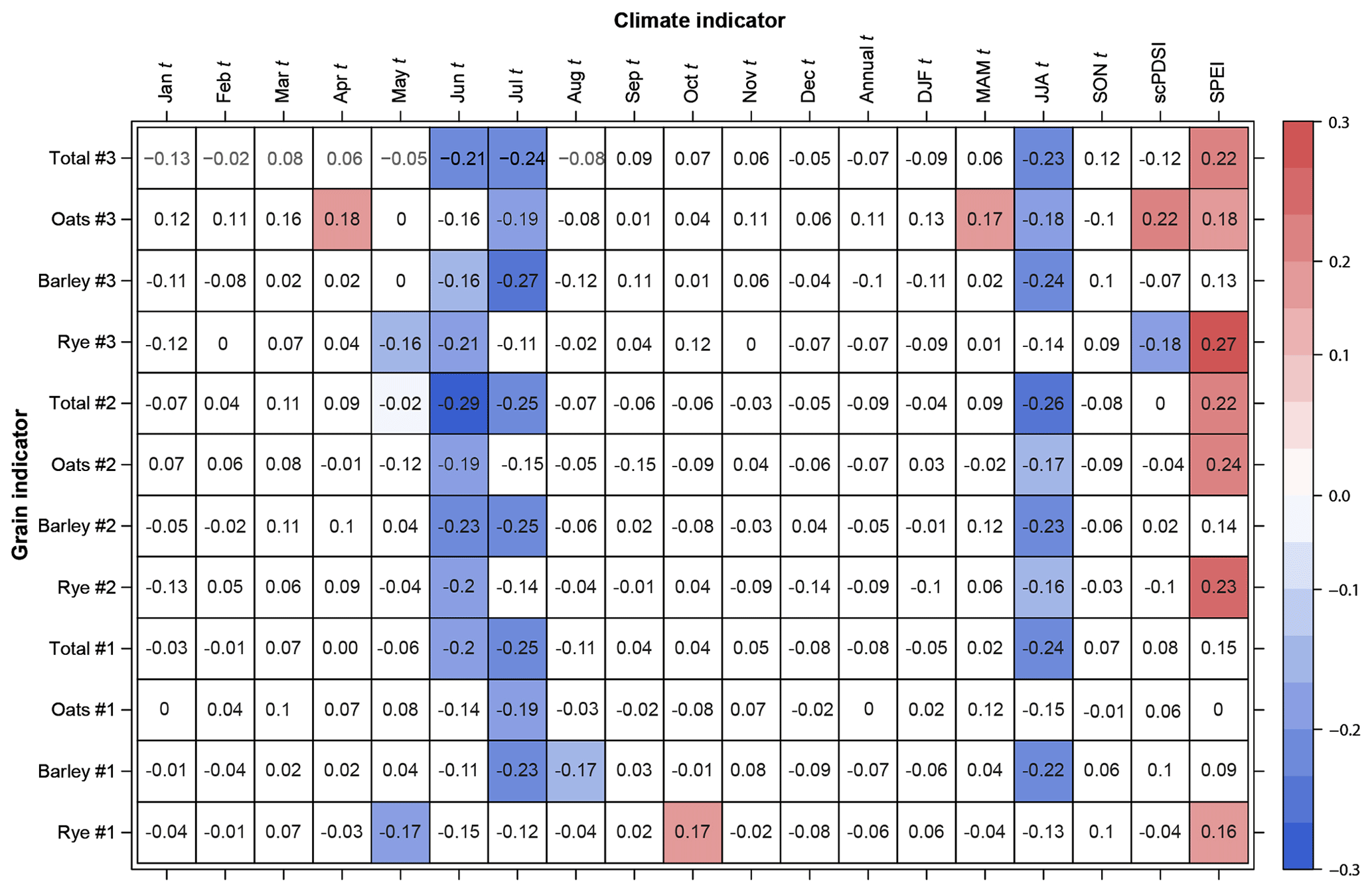
Figure 9Correlations of grain series vs. temperature and hydroclimate indicators, ca. 1702–1865. Note: only statistically significant (p≤0.05) correlations are colored. Clusters are signified by number. Sources: HDSA, Cook et al. (2015), Seftigen et al. (2017), and the homogenized monthly temperature series (Appendix A).
The results revealed by Fig. 10 for monthly summer precipitation show the inverse of those of temperature and hydroclimate: strong positive correlations with grain production. In addition, there are more differences between the various clusters and grains. There are no significant correlations between rye production and the instrumental summer precipitation variables, although in clusters 2 and 3 there is a positive correlation with reconstructed MJJ. On the other hand, there is a negative association between January (and February in cluster 1) precipitation and rye production in all clusters. Barley, oats, and total grain production all show large positive correlations with June and July precipitation and with reconstructed MJJ. The number of rainy days in June and July produce a strong positive signal in relation to almost all grain production, especially barley production, in clusters 2 and 3. There is also a positive, albeit weak, association between the number of rainy days in May and oat production in cluster 2 and rye production in cluster 3.
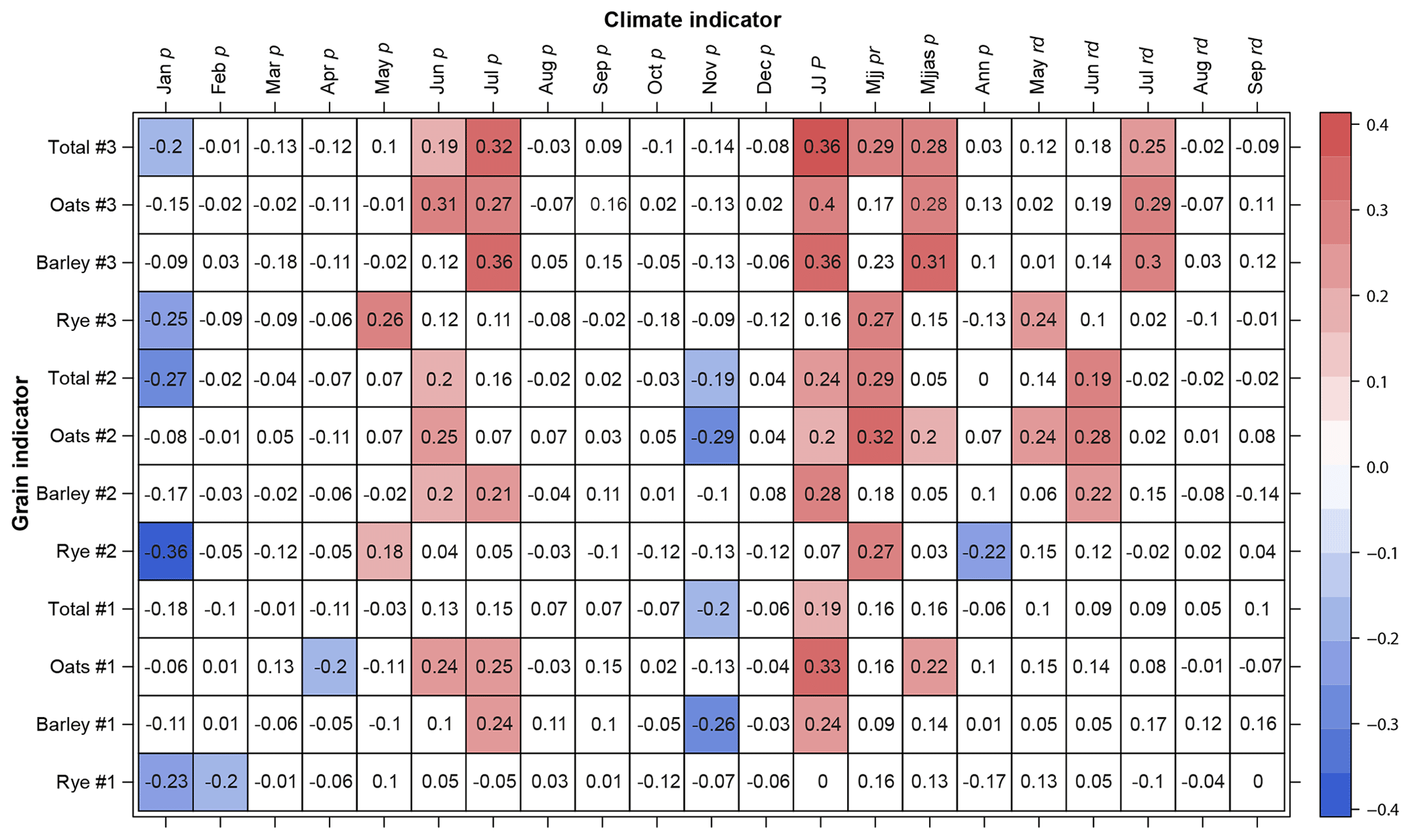
Figure 10Correlations of grain series vs. precipitation indicators, ca. 1748–1865. Note: only statistically significant (p≤0.05) correlations are colored. Clusters are signified by number. Sources: HDSA, Sefitgen et al. (2020), and Tidblom (1876).
Overall, the magnitude of the correlations are similar across grains and climate indicators, except correlations involving barley production that provide the strongest effects. Cluster 3 stands out in relation to the other clusters in producing a stronger signal between most grain production and precipitation.
4.2.2 Grain production and climate variability 1865–1911
The results from the later study period, depicted in Fig. 11, are for the most part consistent with those of the earlier period using the HDSA data, although only for the spring grains (excluding spring rye and spring wheat). Notably, the coefficients are much higher for the latter period compared to the earlier period: roughly double in magnitude. May and to a larger extent June and July temperatures are negatively associated with the series for oats, barley, and mixed grain. Furthermore, maximum and minimum June temperatures also yield negative coefficients. Similar to the 1702–1865 period, the SPEI is positively correlated with the spring grains. The related MJJpr yields positive coefficients which are strong (between r=0.46 for barley and r=0.57 for oats). June precipitation is positive for the three spring grains, whereas no statistically significant results are obtained for July, which is surprising considering the importance of July precipitation in the period 1702–1865. Autumn rye and autumn wheat only show one statistically significant relationship each, with November precipitation for autumn rye () and with MJJpr for autumn wheat (r=0.46).
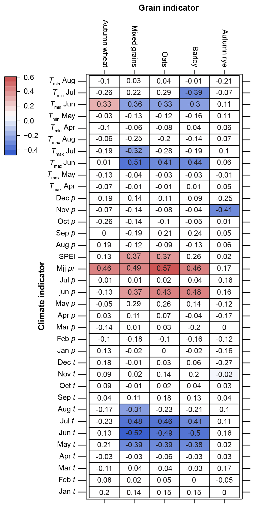
Figure 11Correlations of grain series vs. climate indicators 1865–1911. Note: Only statistically significant (p≤0.05) correlations are colored. Sources: SCB (2021), Seftigen et al. (2017, 2020), and SMHI (2021).
4.2.3 Grain production and climate variability during years with dry and wet summers
Repeating the analysis on restricted samples for which only the years with the driest and wettest summers are included, the direction of the relationships remains consistent. Figure 12 shows the results of the correlation analysis in the early period considering only dry years (as defined by the SPEI). The magnitude of the negative association between summer temperatures and all grain production except for oats increases, yielding correlation coefficients between −0.3 and −0.52.
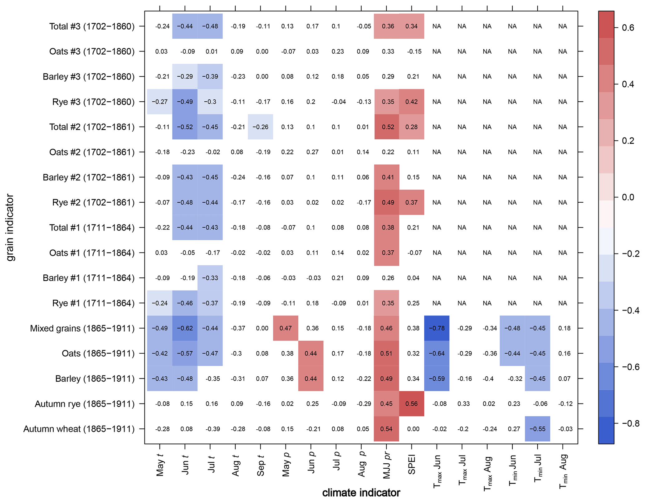
Figure 12Correlations of grain series vs. climate indicators ca. 1702–1865 and 1865–1911 during relatively dry years. Note: only statistically significant (p≤0.05) correlations are colored. Clusters are signified by number. Sources: HDSA, SCB (2021), Tidblom (1876), Seftigen et al. (2017, 2020), SMHI (2021), and the homogenized monthly temperature series (Appendix A).
There is no statistically significant effect from monthly summer precipitation except for the MJJpr, which shows a positive association with most grain production in all clusters except oats in clusters 2 and 3. Considering only wet years in the early period (Fig. 13), summer temperatures are still negatively associated with grain production in all clusters, especially cluster 1. Additionally, there is a positive association between rye production and September temperatures in clusters 2 and 3 in wet years. Notably, the highest correlation coefficients are obtained by the correlation between grain production and precipitation during June, and especially July, during wet years in the early 1702–1865 period (r between 0.31 and 0.78).
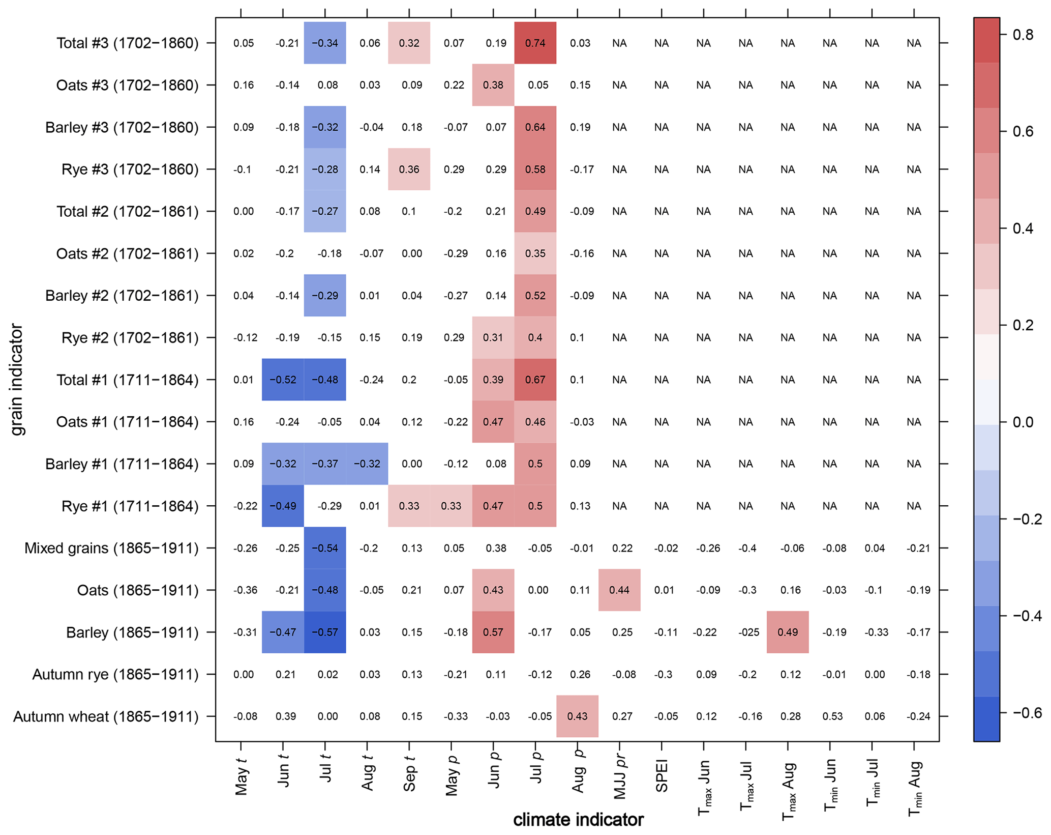
Figure 13Correlations of grain series vs. climate indicators ca. 1702–1865 and 1865–1911 during relatively wet years. Note: only statistically significant (p≤0.05) correlations are colored. Clusters are signified by number. Sources: HDSA, SCB (2021), Tidblom (1876), Seftigen et al. (2017, 2020), SMHI (2021), and the homogenized monthly temperature series (Appendix A).
The main result obtained in this study was the negative association between all grain production and summer temperatures as well as a corresponding positive association with summer precipitation, especially during the high summer months of June and July, in the early study period (1702–1865) and for spring crops in the late study period (1865–1911). Another important finding was the lack of signal for autumn grains in the late study period as well as the weak relationship between autumn and spring temperatures and grain production during the whole study period. Finally, during homogenization of the monthly temperature series from Lund a cold bias was identified in the late 18th century and multiple statistically identified breaks, almost all of which could be associated in time with changes in observers and/or instrument locations. In the following sections, all these results are discussed in more detail.
5.1 The relationship between temperature, precipitation and grain production across the seasons
For roughly 2 centuries, between the early 18th and early 20th centuries, the results of this study show that Scanian grain production had a reversed relationship to temperature compared to other parts of Scandinavia, as well as other parts of Europe (Esper et al., 2017; Pribyl, 2017; Brunt, 2015; Holopainen et al., 2012; Waldinger, 2012; Holopainen and Helama, 2009). This merits some further discussion.
Precipitation and drought during the growing season were pointed to by Utterstörm (1957) and later by Edvinsson et al. (2009) as the primary agrometeorological constraints for pre-industrial agriculture in southern Sweden. Much of the arable land in Scania, as elsewhere in southern Sweden, was situated on well-drained and elevated soils, whereas meadows were often on more low-lying and wet soils (Dahl, 1942; Gadd, 2001). These circumstantial factors, combined with the consistent findings of negative associations with June and July temperatures and positive associations with precipitation in June and July, indicate that summer drought was the greatest agrometeorological risk to grain production. Relative to the benefits of intensive grain production in the region, this was by all accounts a risk worth taking. Indeed, most of the land improvements that occupied farmers in the 19th century after enclosures were about transforming wetter lands to well-drained arable lands, primarily through ditching, rather than efforts to preserve soil moisture (Bohman, 2010).
Nonetheless, it is worth considering what farmers could do to mitigate the risk of drought: in regards to the grain cultivation on well-drained soils, probably very little. It was after all the very same characteristics in the soil that increased the risk of drought that also made a large production of grains possible. Grain production in the cluster with the best soils in this study, cluster 3, showed a relationship with climate variability that was of similar or greater magnitude than the other clusters. Cluster 3 also has the largest share of peasant-owned and crown-owned farms. Theoretically, it can be expected that with increased private ownership of farms, risk-taking will also increase in comparison with tenant farms. One concrete example of such risk-taking would be to make long-term land improvements in the form of drainage. A version of this argument is commonly made in reference to enclosure. Nyström (2018), for example, found that enclosed farms experienced more risk in agricultural production compared to non-enclosed farms in Scania during the period 1750–1850. The results obtained here support the notion that privately owned farms engaged in greater risk-taking. However, a more conclusive affirmation of this hypothesis in the Scanian context would require a more in-depth study of farms with similar soil characteristics but different property rights regimes.
The extensive land reclamation efforts that took place during the 18th and 19th century could have helped mitigate drought as an unintentional and temporary side effect by making new lands of variable qualities, not least in terms of drainage, available (Håkansson, 1997). A diversified composition of grain production also helped to some extent to make grain farming more resilient in Scania. The slight but important variation between the grains in terms of their relationship to summer temperatures and precipitation, with oats and rye more sensitive to variation in May and in particular June and barley more sensitive to variation in July, accordingly spread out risks. Diversity within each grain variety would also have been helpful in mitigating the risk to drought or other climate anomalies (Hagenblad et al., 2012, 2016; Leino, 2017; Lundström et al., 2018).
As noted in Sect. 1.4, Edvinsson et al. (2009) suggested that before the agrarian transformations in the 18th and 19th centuries, yields were in general so low as to lead to a chronic shortage of seeds, which they suggested overrode the effects from climate variability and hence the weak relationship between temperatures and grain yields. Theoretically, low yields leading to low seed quantities could obfuscate the effect of temperature, necessitating some kind of control for the previous year's weather. For example, Bekar (2019) found that English manorial harvests in the 13th and 14th centuries were persistent, i.e., subpar harvests, partly induced by “weather shocks”, persisted into the subsequent year for both wheat and other grain crops like barley and oats. Notwithstanding these results, the relevance of 14th century England for 18th century Scandinavia is arguably limited. In instances in which one might assume persistent harvests would be more apparent (although it is arguably an understudied phenomenon), like northern Finland, one still finds strong current-year temperature effects on grain yields and production during the early modern period (Huhtamaa and Helama, 2017b; Huhtamaa, 2015; Solantie, 1988). Having limited amounts of seed did not obfuscate or exclude the effects from weather. Rather, the evidence seems to suggest it made farmers more vulnerable and the effects more apparent. There are few reasons to suspect that chronic seed shortages were a major issue in 18th century Scania, given that it was mostly an exporter of grains and experienced more or less ongoing increases in production during the period (Olsson and Svensson, 2010).
In relation to this argument, I would highlight another important result of this study, namely the absence of a climate signal in the spring and autumn months, as well as the last summer month of August to some extent. In the neighboring lands of Denmark, Huhtamaa and Ljungqvist (2021) suggest that it is possible that frosts were not a major problem, even in the wetter and colder periods of the LIA. The results from Sect. 3.1.2 show that the average date for the first occurrence of autumn frost in Lund was 8 November and not earlier than October in the northernmost areas of Scania, well after the harvest month of August as well as the sowing of autumn rye. In many years there were no spring frosts later than March, whereas in those years when they occurred after March the average date was 15 April in Lund. In the highlands in the north, spring frosts on average occurred later. Nonetheless, spring frosts, when they occurred, generally did so just before or at the start of the growing season. Thus, the results in this study point to spring and autumn frosts not being a systematic threat to grain production, except in localized conditions. An implication of this is that the combination of the climate in Scania with the farming systems Scanian farmers adhered to offered good margins for the spring and autumn agricultural work seasons, for example by allowing for delays in sowing and harvesting.
Based on the findings in this study, I would revise the notion forwarded by Utterström (1957) and Edvinsson et al. (2009). It was not only precipitation but rather the combination of temperature and precipitation during the summer that constituted the main constraints for the production of spring grains during the whole study period and for all grains in the early study period. Furthermore, I would not only frame the relationship in the form of constraints and risks. Grain farming in Scania was adapted to, and benefitted by, cool and humid summer conditions. Even in years with wet summers there was a positive association between grain production and summer precipitation and a negative association between the former and summer temperatures. This would likely also be the case in other parts of southern Sweden where similar grain varieties were cultivated in the same type of farming systems on well-drained soils. In the later study period, both maximum and minimum June and July temperatures were negatively correlated with the production of spring grains, suggesting an optimal temperature range for these crops during these months and that the occurrence of extreme cold and heat had some detrimental effect.
5.2 The role of grain varieties
An account of the relationship between grain production and climate variability has to account for the type and varieties of grains being cultivated as well as the farming system more broadly. In Scania in the late 19th century, new autumn grain varieties, similar to those on the European continent, gradually replaced the old varieties that were more similar to those in other parts of Fennoscandia. I argue that this, rather than changes in the climate, was the most likely cause behind the diminished signal in the relationship between climate variability and autumn grains in the latter study period, given that the relationship with climate variability remained intact for most of the spring crops. Edvinsson et al. (2009) also argued that the shift towards new grain varieties changed the underlying relationship between grain production and climate variability from a negative to a positive association with temperatures, especially in the spring and early summer. The farming systems of Scania likewise underwent changes whereby arable lands were expanded and intensified with new crop rotations, land improvements, increased drainage, external sources of fertilizer, and burgeoning mechanization. All these changes created conditions that were more favorable for the new grain varieties.
Nonetheless, it is possible that climate changes over a longer timescale were an active driver in the relationship between climate variability and grain production, considering that the historical grain varieties were changeable and adapted to changing circumstances, not least climate variability at different timescales (Leino, 2017). It can be argued that farming in Scania during the 17th up until the late 19th century had adapted over time to a more cool and humid summer climate, having experienced multiple cold years and extended periods with reduced average temperatures during the LIA in the 16th and 17th centuries, possibly earlier as well. Current evidence suggests that the grain varieties cultivated during these centuries were similar to or of the same group of varieties grown in more northerly and cold latitudes. For example, in regards to rye, Larsson et al. (2019) found through genetic analysis of preserved Fennoscandian rye seeds that they all belonged to the same meta-population of rye landraces that had been stable for at least the last 350 years. Similarly, Aslan et al. (2015) found that barley landraces from Fennoscandia form a homogenous group of barley landraces, distinct from other parts of Europe. This particular group of northern European barley varieties carries the nonresponsive ppd-H1 allele that prolongs flowering when exposed to periods with increasing daylight hours. Presumably, this would be beneficial during cooler and wetter periods by taking full advantage of the extended growing season. Studies of modern Finnish barley cultivars have shown that yields for most varieties are negatively correlated with excess rain or drought around the sowing season and positive in the subsequent stages of crop development, whereas they are negatively correlated with temperature at most stages of crop development, especially before heading (Hakala et al., 2012). The homogeneity of barley landraces over time in southern Sweden was confirmed by Lundström et al. (2018), who traced it back to at least the late 17th century. While Lundström et al. (2018) argued that such homogeneity was maintained despite repeated crop failures in southern Sweden between the 1700s and the 1900s, I would argue, at least when considering Scania, that such homogeneity was probably maintained because of the lack of repeated crop failures.
The discussion of the results on the relationship between specific grains and climate variability should also be put in a broader perspective. In terms of crop composition and the type of field system (a Swedish variant of the open-field systems called tegskifte), the farming systems of Scania remained more or less the same until the 19th century, when enclosure and new crop rotation systems started to be introduced, starting in the plains districts. All the same, even after the introduction of new crop rotations, which normally meant increasing shares of fodder crops, in Scania grain production continued to retain its primacy, at least in the plains districts (Bohman, 2010). This motivates the argument that the farming systems of Scania overall were resilient to colder conditions, at least until the late 19th century, given the importance of grain production. However, the relationship between livestock production, total agricultural production, and climate variability would require a study of its own.
5.3 Implications of the late 18th century cold bias and ACMANT detected breaks
Previous research that identified increasing soil erosion and sand drift in Scania during the 18th century partly blamed the coldness of the last 4 decades of the 18th century as indicated by the instrumental temperature measurements taken in Lund (Mattsson, 1987). After homogenization of the Lund temperature series 1753–1870, the largest corrections due were for upwards adjustments for summer temperatures in the same period, i.e., the late 18th century. In other words, the results suggest that the ca. 1770–1800 period was not as cold as suggested by Mattsson (1987) or the unhomogenized Lund temperature series. While these findings speak against a regional climate-driven ecological crisis, they do align with the results of Bohman (2017a, b), who downplayed the spatial scale of the ecological crisis, emphasizing its local and conditional character, as well as the counteracting efforts by local communities and authorities.
The breaks detected through the ACMANT procedure could almost all be associated with changes in observers and/or instrument location. While there is uncertainty in the number of times the instruments were replaced, those known could not be associated in time with the detected breaks. This suggests that the human factor, i.e., the degree of consistency in training, skills, and interest in observers, was the primary determinant in measurement quality and homogeneity. Faulty instruments or station location biases could in the end only be perceived, understood, and subsequently corrected or adjusted for by the human observer. The first decades, 1753–1774, can be considered a period of more competent (meteorological) observers, followed by the period after ca. 1850 when training and methodologies in meteorological observations had improved. Nonetheless, for most of the homogenization period there were issues of inhomogeneity requiring corrections.
5.4 Hydroclimate and historical grain production
Three different hydroclimate reconstructions were employed for this study. In the early period (1702–1865) very few and mostly inconsistent results were obtained using the scPDSI from the OWDA (Old World Drought Atlas), and no statistically significant results were found for the late period (1865–1911). The SPEI from Seftigen et al. (2017) was found to be positively associated with most grain production except barley, consistent over different samples and periods as well as with results from instrumental precipitation. The results of the MJJpr and SPEI could be interpreted as more important for estimating hydroclimatic conditions relevant for grain production in the early summer (May and June, in particular). This is supported by the lack of statistically significant effects found between May and June climate variables and barley production as well as the fact that the most important month for barley seems to have been July, at least in the early period. This also offers an explanation as to why sorting dry and wet periods with the SPEI indicator led to much larger associations between precipitation and temperature in June and July with grain production. If conditions were wet or dry in the early summer, the effects from subsequent temperature and precipitation later in June and especially July would theoretically have been amplified. A similar argument was made by Brunt (2004), who showed that it was more beneficial to have precipitation spread out during the growing season. An important caveat to these interpretations is that a large degree of uncertainty remains as to what specific hydroclimate effects are captured by or represented in these reconstructions, beyond MJJ or JJA averages. Nonetheless, there does seem to be a relationship between the conditions for tree growth in southern Sweden as represented in these reconstructions and grain production in Scania during the study period. Seftigen et al. (2015) asserted that even though most high-resolution climate proxies in northern-latitude regions are temperature-based, there is also a need for precipitation-based proxies due to the importance of precipitation patterns for economic sectors such as agriculture. The results obtained here confirm both the importance of precipitation patterns for agriculture and the relevance of the proxy reconstructions in studying that relationship.
This article demonstrates the possibilities of estimating the relationship between climate variability and grain production in Scania during the pre-industrial period using available grain production data, climate reconstructions, and the network of early instrumental records. Grain production in Scania did not show any systematic relationship or vulnerability to climate variability in the spring and autumn seasons, whereas a more clear signal could be detected between grain production and climate variability during the summer season, especially in the months of June and July. Until the introduction of new varieties of autumn crops in the late 19th century, grain production was benefitted by cool and wet conditions throughout the summer, although there was a slight but important differentiation between rye and oats, which were more sensitive to conditions in May and June, and barley, which was mostly sensitive to conditions in July. The most apparent agrometeorological risk was summer drought. However, severe droughts like the one in the summer of 2018 were rare in Scania and the diversification within and between historical grain varieties cultivated meant that, by and large, this risk was manageable, especially when compared to the benefits of intensive grain production in the region. Scania largely conforms to the previous, albeit sparse, picture in the Swedish historiography of the relationship between historical grain production and climate in southern Sweden. At the same time it stands out compared to studies of other parts of Scandinavia and continental Europe wherein positive associations between grain production and summer temperatures have been identified.
The results obtained here should be further developed by integrating them into a broader model of the impacts of climate variability on agriculture, with other factors, e.g., market prices and access as well as institutional and other geographical factors like soil conditions, formally accounted for. This need is not least implied by the fact that even in the confined geographical area of Scania there was differentiation among sets of villages in regards to the relationship between their grain production and climate.
Daily meteorological observations began in Lund in 1740, spearheaded by the professor of mathematics Daniel Menlös. Systematic instrumental meteorological observations began in 1747 for precipitation and late 1752 for temperature and air pressure under the responsibility of a formally appointed observer. Naturally, these observers changed over time. Instruments were also replaced or upgraded on a few occasions. More problematic from a perspective of consistency and reliability, the location of the instruments also changed multiple times. There is also a gap in (quality) temperature measurements between the years 1821 and 1833 as well as some other minor gaps over the period 1753–1870 (see Fig. A1). Issues relating to the nonhomogeneity of these meteorological series, not least the temperature series, were already partly identified and discussed in the 19th century by Tidblom (1876). Schalén et al. (1968) and Bärring et al. (1999) also discussed inhomogeneities in the series relating to the station history.
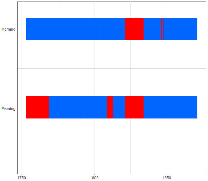
Figure A1Gaps in the Lund temperature series, 1753–1870. Source: Tidblom (1876). Note: blue signifies available data and red signifies a gap. Measurement units are in the form of pentad (5 d) averages.
Tidblom (1876) published the Lund temperature series in the form of pentad averages. He removed the daytime measurements and used only the morning and evening measurements, arguing that these were less affected by the location of the thermometer. He also did some minor manual corrections for September through December in 1834 and individual days in June in 1842 and 1843. Overall, the adjustments made by Tidblom (1876) should be considered minor and it seems probable that inhomogeneities remain in the series. Nonetheless, the temperature series have subsequently been employed in at least a few historical studies. For example Palm (1997) used the series to estimate the impact of temperature variations on grain yields on a farm in Halland, southwestern Sweden, during the years 1758–1865. To fill in the gaps Palm bridged the Lund series with data from Copenhagen using average differences. Mattsson (1986) observed the trends in the Lund series and argued that a reduction in temperatures in the last 3 decades of the 18th century, combined with changes in wind patterns, contributed to widespread soil erosion in Scania during the 18th and early 19th centuries. Using inhomogeneous data sets carries many important drawbacks, not least the risks of spurious and unreliable results (Aguilar et al., 2003). Hence, it is necessary for the purposes of this study to homogenize the temperature series.
Given that the exact location and relocations of the measurements for the period up until 1780 are unknown, it is difficult to identify periods of measurement error and estimate correction coefficients manually. The most tested approaches for homogenization of temperature series involve using interpolation techniques relying on homogenized data from nearby stations or networks of stations (Venema et al., 2012). It is generally advisable to use more than one station for interpolation since it reduces the probability of a single station bias as well as the general reliability of the interpolation (Conrad and Pollak, 1950). Again, applying interpolation manually is problematic since it risks introducing new biases for the less detailed parts of the Lund measurement station history. There are also computational difficulties in manually interpolating from a network of stations. Therefore, I employ the adapted Caussinus–Mestre algorithm for homogenizing Networks of Temperature Series (ACMANT) software. ACMANT relies on a homogenized network of stations and a computationally efficient algorithm for homogenizing climate data and data infilling.
I use a network of homogenized monthly temperature series located in the northwestern part of Europe for the homogenization process, namely Berlin–Dahlem (from 1719 with a gap between 1722–1727), central England (from 1659), Copenhagen (from 1768 with gaps between 1777–1781 and 1789–1797), De Bilt (from 1706), Stockholm (from 1756), and Uppsala (from 1722) (DWD, 2018; Bergström and Moberg, 2002; Cappellen et al., 2019; Moberg et al., 2002; van Engelen et al., 2001; Labrijn, 1945; Parker et al., 1992; van Engelen, 1995; Manley, 1973). Given that spatial correlations in temperatures on a daily or weekly basis are lower across the network region compared with monthly or seasonal averages and that daily temperature series are not available at all network stations, I employ monthly averages for homogenization. The ACMANT homogenization procedure requires spatial correlation coefficients of at least 0.4 with network stations and a minimum of four network time series. Spatial correlation coefficients are calculated from the increments in the time series after monthly climatic means have been removed (Domonokos and Coll, 2017). Table A1 shows the descriptive statistics of the network stations, including monthly correlations and spatial correlations.
Table A1Correlations between monthly temperatures in Lund and other network series.
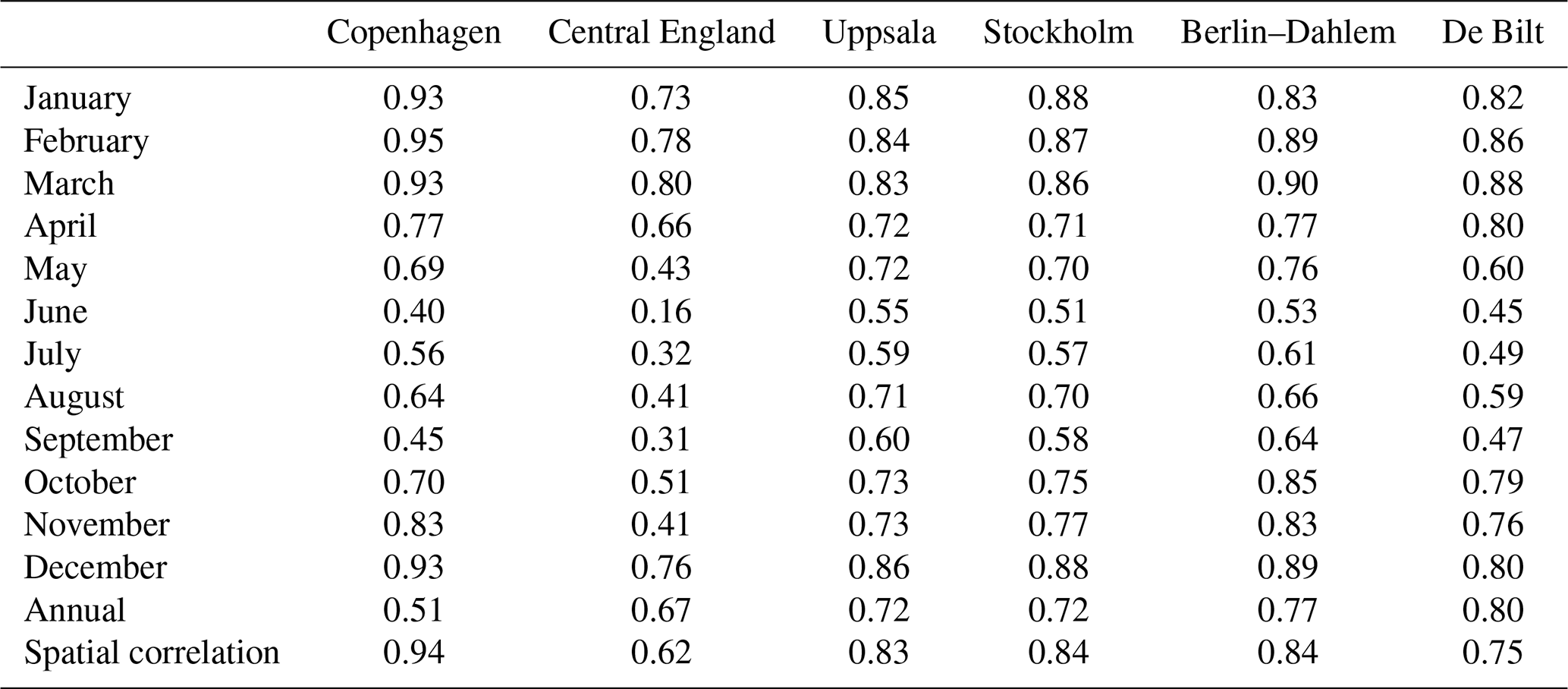
Sources are as follows: Central England (Manley, 1973, Parker et al., 1992), Copenhagen (Cappelen et al., 2019), Berlin–Dahlem (DWD, 2018), De Bilt (Durre et al., 2008; Lawrimore et al., 2011), Lund (Tidblom, 1876), Uppsala (Bergström and Moberg, 2002), and Stockholm (Moberg et al., 2002; Moberg, 2021). Note that spatial correlation coefficients are obtained by ACMANT, with increment series correlated after monthly climatic means have been removed (Domonokos and Coll, 2017).
A1 Detected breaks and station history
The ACMANT homogenization procedure detects eight breaks in the Lund temperature series. These breaks can be interpreted in light of what is known about the station history. Figure A2 shows known or suspected relocations and changes in observers between 1753 and 1870 as well as the detected breaks (Nenzelius, 1775; Tidblom 1876; Schalén et al., 1968; Bärring et al., 1999).
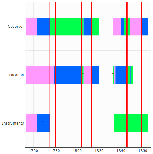
Figure A2Station history and ACMANT-detected breaks, 1753–1870. Sources: Tidblom (1876), Schalén et al. (1968), and Bärring et al. (1999). Note: each colored area represents a distinct period location, observer, or set of instruments. denotes multiple changes during the indicated period. Detected breaks are shown by the vertical red lines. Gaps in white signify missing data.
For the first 22 years, no breaks are detected, even though there is one change in observer (1763) and several replacements of instruments. The location of the instruments appears to have been constant. Furthermore, in 1770 there was a Royal Ordinance that the results from all monthly meteorological observations were to be sent in to the Swedish Royal Academy of Sciences. The first 2 decades of measurements were published by the Swedish Royal Academy of Sciences (Nenzelius, 1775). It is possible that the attention and interest given to meteorological observations as a preeminent scientific venture at this particular moment in time led the first two observers, Nils Schenmark and Olof Nenzelius, to make serious efforts to make sure the series was consistent or as correct as possible. Tidblom (1876) argued that were was no reason to suspect that the instruments or observers were lacking in quality or skill, at least during Schenmark's time (1753–1763). In the 1770s, there are some intermittent notes from this period of corrections to faulty instruments, something that is much sparser in the subsequent period (Tidblom, 1876).
The first detected break occurs in 1775, the same year in which Anders Lidtgren and his assistant Pehr Tegman took over observation responsibilities. It is possible that the thermometer also changed location at this time. Another break occurs in 1780, approximately coinciding with the change in location for the instruments in late 1779 to the upper story of Kungshuset. In 1798, 1804, and 1813 there are further breaks detected in the series. Nothing formally appears in the station history that could explain the 1798 break. However, the responsible observers, A. Lidtgren and P. Tegman, were both increasingly occupied with other duties, suggesting that actual meteorological observations were undertaken by some other unknown assistant. P. Tegman became a professor of mathematics in 1787, was awarded membership in the Royal Swedish Academy of Sciences in 1795, and was awarded membership in the board of mathematics in 1798. Furthermore, he was appointed dean of Lund University in 1795 and became responsible for a church deanery in 1797. A. Lidtgren was also awarded membership in the board of mathematics in the Royal Swedish Academy of Sciences in 1798 (Ståhl, 1834; Dahlgren, 1915). A. Lidtgren was recognized for his work in astronomy and astronomical observations, whereas much less is known about his work with meteorological observations (Dahl, 1948). Unlike their predecessors, neither P. Tegman nor A. Lidtgren made any publications regarding meteorological observations.
Both the 1804 and 1813 breaks occur during times of more apparent and known changes in the station history. In 1804 the instruments changed location several times, and in 1813 there was a change in observer to Adolph Frederic Knieberg, who supposedly also relocated the instruments to his living residence (Tidblom, 1876). Finally, there are detected breaks in 1845, 1846, and 1859. Between the 1820s and mid-1830s the instruments changed location on a number of occasions (leading to the gap in the temperature series between 1821 and 1833 due to the low quality of the temperature data in that period). The location of the instruments is then not mentioned in the records until 1846 when they again appear to have changed location. In 1858, there was a change in observers, but there are no changes in location close in time to the 1859 break.
Thus, almost all detected breaks occur in the same year as or the subsequent year to a change in observer or station location. Furthermore, almost all known changes in station location and observers are detected as breaks, at least in the 18th century. The largest exception is the break in 1845 that occurs more than a year after the latest known change in the station history, which is when there was a change in observer in 1843. However, in 1846 there is both a station relocation and a detected break. The latest detected break occur in 1859, shortly after a change in observers in 1858.
Overall, the change in instruments appears to have been a less important factor in causing inhomogeneities in the series compared with changes in observer and instrument location. Not one of the known changes in thermometers occurred at a point in time proximate to a detected break. Presumably, if an instrument was faulty the more skilled observers, as is noted on several occasions in the station records, could correct for this. Similarly, an unskilled or careless observer would have been less likely to identify faulty instruments, accurately read and note down observations, and appreciate the consequences of moving the instruments to a particular location (see Pfister et al., 2019, who discuss issues related to the maintenance of reliable and consistent observers).
Table A2Average time of day for morning and evening measurements, 1753–1870.
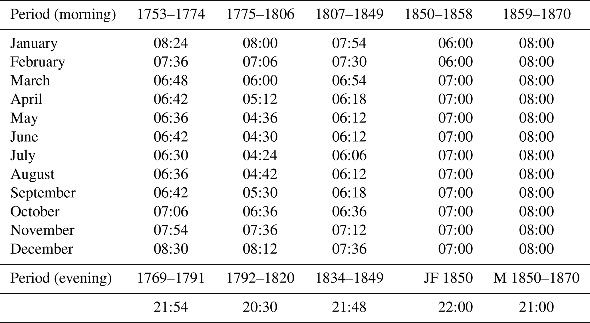
Source: Tidblom (1876). Note: single letters in the “Period” row denote months; e.g., JF denotes January–February.
A2 The late 18th century cold bias
As shown in Figs. 7 and 8, the largest corrections in the homogenization procedure occurred during the summer months and to a lesser extent spring months of the last decades of the 18th century, signified by the two detected breaks in 1775 and 1780 (Fig. A2). Other studies attempting to homogenize early instrumental temperature series have also found summers to be a larger source of measurement bias compared with the other seasons. For example, when performing manual testing during homogenization of the Stockholm instrumental temperature series (beginning in 1756) Moberg et al. (2002) noted, in line with Modén (1963), that the largest discrepancies due to station location were to be observed during the summer months. Dobrovolný et al. (2010) also found a similar seasonal pattern in their study of early instrumental temperature series in central Europe. They argued that thermometers, which during the late 18th and early 18th century were mostly placed in a north-facing direction and without proper sheltering, were subject to a systematic summer season warm bias. They also conceded that this bias differed for different stations, depending on latitude, altitude, and other station-specific conditions.
In the Lund early instrumental period, particularly in the late 18th century, it appears conditions were reversed from those in central Europe; namely, there is a cold bias during the summer season as well as the during the growing season (AMJJAS) as a whole. Across the entire homogenization period, there is a slight correction upwards for spring and summer temperatures, which can be explained by the use of morning and evening observations, excluding daytime observations. To explain the much larger corrections made from 1775 until 1804 one has to consider the specifics of the station history during that period. During the years 1775–1806, the average time of the morning observations occurred up to 2 h earlier during the months of MJJA compared to the previous period 1753–1774. For the other months of the year the differences were much smaller; see Table A2. Furthermore, in late 1779 the thermometer was moved to the upper room of the Kungshuset, located at an altitude of 61m. Bärring et al. (1999) argue that these facilities probably were unheated until the 1830s. Given these conditions, it is feasible that the thermometer location between 1779 and 1804 was colder than the preceding and succeeding locations.
Thus, a consideration of the specifics of the station history, notably the change in observers, observation practices, and station relocation, in combination with the homogenization results, suggests that the Lund temperature series exhibits a cold bias in the last decades of the 18th century. This result has bearing on historical climate reconstructions generally, but also for the agrarian and climate history of Scania and southwestern Sweden, specifically, as discussed in Sect. 4.3 (Mattsson, 1986; Palm, 1997; Bohman, 2017a, b).
Table B1Years at or below the 33th percentile of SPEI (drier conditions) during the years 1702–1865.
Source: Seftigen et al. (2017).
Table B2Years at or above the 67th percentile of SPEI (wetter conditions) during the years 1702–1865.
Source: Seftigen et al. (2017).
Table B3Years below the median of SPEI (drier conditions) during the years 1865–1911.
Source: Seftigen et al. (2017).
Table B4Years above or at the median of SPEI (wetter conditions) during the years 1865–1911.
Source: Seftigen et al. (2017).
The original data used for this article can all be obtained through publicly available repositories, except for the historical temperature data from Copenhagen, which since 2019 is only available upon request; see below. The homogenized monthly mean temperature series compiled as part of this paper is available through request to the author.
HDSA data and related files can be obtained from the repository website of the Department of Economic History at Lund University; see https://www.lusem.lu.se/economic-history/databases/economic-history-data/historical-database-of-scanian-agriculture (last access: 26 January 2022). See also as Olsson and Svensson (2017a; https://lup.lub.lu.se/record/94f24113-f810-4c1d-bd34-22405e41185b, last access: 23 April 2021) for a detailed description of the data.
Lund temperature and precipitation data are available in published format in Tidblom (1876) and are also available in digitized format upon request to the author. Furthermore, monthly precipitation data for Lund are available at the SMHI open data repository, https://www.smhi.se/data/meteorologi/ladda-ner-meteorologiska-observationer#param=precipitationMonthlySum,stations=all,stationid=53430 (last access: 26 January 2022, SMHI, 2021).
De Bilt monthly mean temperature data can be obtained from the Global Historical Climatology Network monthly (GHCNm v3), https://www.ncei.noaa.gov/pub/data/ghcn/v3/, last access: 26 January 2022. See Lawrimore et al. (2011, https://doi.org/10.1029/2011JD016187) for a description of the data.
Central England monthly mean temperature data can be obtained from the Met Office Hadley Centre data repository for observation datasets, https://www.metoffice.gov.uk/hadobs/hadcet/ (last access: 26 January 2022). See Parker et al. (1992, https://doi.org/10.1002/joc.3370120402) and Manley (1974, https://doi.org/10.1002/qj.49710042511) for a description of the data.
Historical monthly mean temperature data from Copenhagen data can be obtained by contacting the customer service of the Danish Meteorological Institute (DMI), see http://research.dmi.dk/data/ (last access: 26 January 2022). For a description of the data, see Cappelen et al. (2019).
Berlin–Dahlem temperature data can be obtained from the open data repository of the Deutscher Wetterdienst (DWD), available at https://opendata.dwd.de/climate_environment/CDC/observations_germany/climate/monthly/kl/historical/ (last access: 2 February 2022). See also DWD (2018).
The contact author has declared that there are no competing interests.
Publisher's note: Copernicus Publications remains neutral with regard to jurisdictional claims in published maps and institutional affiliations.
This article is part of the special issue “International methods and comparisons in climate reconstruction and impacts from archives of societies”. It is not associated with a conference.
I would like to thank the anonymous referees and the editor for their valuable comments.
This paper was edited by Chantal Camenisch and reviewed by three anonymous referees.
Ađalsteinsson, S. and Jensén, P.: Influence of temperature on root development and phosphate influx in winter wheat grown at different P levels, Physiol. Plantarum, 80, 69–74, https://doi.org/10.1111/j.1399-3054.1990.tb04376.x, 1990.
Aguilar, E., Auer, I., Brunet, M., Peterson, T. C., and Wieringa, J.: Guidelines on climate metadata and homogenization, WMO-TD No. 1186, 2003.
Åmark, K.: Spannmålshandel och spannmålspolitik i Sverige 1719–1830, Stockholm, 1915 (in Swedish).
Appleby, A.: Epidemics and Famine in the Little Ice Age, J. Interdiscipl. Hist., 10, 643–663, https://doi.org/10.1515/9781400854103.63, 1980.
Aslan, S., Forsberg, N. E. G., Hagenblad, J., and Leino, W. M.: Molecular Genotyping of Historical Barley Landraces Reveals Novel Candidate Regions for Local Adaption, Crop Sci., 55, 2766–2776, https://doi.org/10.2135/cropsci2015.02.0119, 2015.
Bärring, L., Jönsson, P., Achberger, C., Ekström, M., and Alexandersson, H.: The Lund Instrumental Record of Meteorological Observations: Reconstructions of Monthly Sea-level Pressure 1780–1997, Int. J. Climatol., 19, 1427–1443, https://doi.org/10.1002/(SICI)1097-0088(19991115)19:13<1427::AID-JOC429>3.0.CO;2-H, 1999.
Beillouin, D., Schauberger, B., Bastos, A., Ciais, P., and Makowski, D.: Impact of extreme weather conditions on European crop production in 2018, Philos. T. Roy. Soc. B, 375, 20190510, https://doi.org/10.1098/rstb.2019.0510, 2020.
Bekar, C. T.: The Persistence of Harvest Shocks in Medieval England, J. Econ. Hist., 79, 954–988, https://doi.org/10.1017/S0022050719000524, 2019.
Bergström, H. and Moberg, A.: Daily air temperature and pressure series for Uppsala 1722–1998, Clim. Change, 53, 213–252, https://doi.org/10.1023/A:1014983229213, 2002 (data available at: https://www.smhi.se/data/meteorologi/temperatur/uppsalas-temperaturserie-1.2855, last access: 29 April 2021).
Bohman, M.: Bonden, bygden och bördigheten: Produktionsmönster och utvecklingsvägar under jordbruksomvandlingen i 60 Skåne ca 1700–1870, dissertation, Lund University, Lund, ISBN: 9789174730142, 2010 (in Swedish).
Bohman, M.: Tionde och vad mera dem med rätta tillkommer.: Prästtiondelängder som källmaterial för studier av bondejordbrukets djurhållning under 1700- och 1800-talets agrara revolution, Hist. Tidsskr., 132, 448–482, 2012 (in Swedish).
Bohman, M.: Conditional Crisis? Ecological challenges and conditions of growth during the agricultural revolution in southern Sweden, c. 1700-1900. Econ. Hist. Rev., 70, 171–186, https://doi.org/10.1111/ehr.12335, 2017a.
Bohman, M.: Deal with it!: The emergence and reversal of an agro-ecological crisis, Southern Sweden in the eighteenth and nineteenth centuries, Scandinavian Economic History Review, 65, 206–220, https://doi.org/10.1080/03585522.2017.1286257, 2017b.
Bremensis, A.: History of the Archbishops of Hamburg-Bremen: Columbia University Press, 2002.
Bringéus, N. A.: Sockenbeskrivningar från Malmöhus Län 1828. Arcus Förlag, 2013 (in Swedish).
Brunt, L.: Nature or Nurture? Explaining English Wheat Yields in the Industrial Revolution, c.1770, J. Econ. Hist., 64, 193–225, https://doi.org/10.1017/S0022050704002657, 2004.
Brunt, L.: Weather shocks and English wheat yields, 1690–1871, Explor. Econ. Hist., 57, 50–58, https://doi.org/10.1016/j.eeh.2014.12.001, 2015.
Camenisch, C.: Endlose Kälte – Witterungsverlauf und Getreidepreise in den Burgundischen Niederlanden im 15. Jahrhundert, in: Wirtschafts-, Sozial- und Umweltgeschichte (WSU), 5, 530 pp., https://doi.org/10.24894/978-3-7965-3474-4, 2015 (in German).
Campbell, Å.: Skånska bygder under förra hälften av 1700-talet: etnografisk studie över den skånska allmogens äldre odlingar, hägnader och byggnader, Lundequistiska bokhandeln, Uppsala, 1928 (in Swedish).
Campbell, Å.: Det svenska brödet: en jämförande etnologisk-historisk undersökning, Svensk bageritidsskrift, Stockholm, 1950 (in Swedish).
Cappelen, J., Kern-Hansen, C., Laursen, V. E., Jørgensen, V. P., and Jørgensen, V. B.: Denmark – DMI Historical Climate Data Collection 1768–2018, DMI Report 19-02, Danish Meteorological Institute, ISSN: 2445-9127, 2019 (data available at: http://research.dmi.dk/data/, last access: 26 January 2022).
Cockram, J., Jones, H., Leigh, F. J., O'Sullivan, D., Powell., W., Laurie, A. D., and Greenland, A. J.: Control of flowering time in temperate cereals: genes, domestication, and sustainable productivity, J. Exp. Bot., 58, 1231–1244, https://doi.org/10.1093/jxb/erm042, 2007.
Conrad, V. and Pollak, C.: Methods in climatology, Harvard University Press, Cambridge, MA, 459 pp., ISBN 9780674187856, 1950.
Cook, E. R., Seager, R., Kushnir, Y., Briffa, K.R., Buntgen, U., Frank, D., Krusic, P. J., Tegel, W., van der Schrier, G., Andreu-Hayles, L., Baillie, M., Baittinger, C., Bleicher, N., Bonde, N., Brown, D., Carrer, M., Cooper, R., Cufar, K., Dittmar, C., Esper, J., Griggs, C., Gunnarson, B., Gunther, B., Gutierrez, E., Haneca, K., Helama, S., Herzig, F., Heussner, K.-U., Hofmann, J., Janda, P., Kontic, R., Kose, N., Kyncl, T., Levanic, T., Linderholm, H., Manning, S., Melvin, T.M., Miles, D., Neuwirth, B., Nicolussi, K., Nola, P., Panayotov, M., Popa, I., Rothe, A., Seftigen, K., Seim, A., Svarva, H., Svoboda, M., Thun, T., Timonen, M., Touchan, R., Trotsiuk, V., Trouet, V., Walder, F., Wazny, T., Wilson, R., and Zang, C.: Old World megadroughts and pluvials during the Common Era, Science Advances, 1, e1500561, https://doi.org/10.1126/sciadv.1500561, 2015.
Dahl, S.: Torna och Bara. Studier i Skånes bebyggelse-och näringsgeografi före 1860, Carl Bloms boktryckeri, 1942 (in Swedish).
Dahl, S.: Studier i äldre skånska odlingssystem, Meddelanden från Kulturgeografiska institutionen vid Stockholms universitet, 0585-3508;B 6969, Stockholm, 1989 (in Swedish).
Dahl, T.: Svenska män och kvinnor: biografisk uppslagsbok, Vol. 4, I – Lindner, Bonnier, Stockholm, 1948 (in Swedish).
Dahlgren, E. W.: Kungl. Svenska Vetenskapsakademien: Personförteckningar 1739–1915, Almquist & Wiksells boktryckeri, Stockholm, 1915 (in Swedish).
Day, H. E. W. and Edelsbrunner, H.: Efficient algorithms for agglomerative hierarchical clustering methods, J. Classif., 1, 7–24, https://doi.org/10.1007/BF01890115, 1984.
Degroot, D.: Towards a rigorous understanding of societal responses to climate change, Nature, 591, 539–550, https://doi.org/10.1038/s41586-021-03190-2, 2021.
de Vries, F. T., Griffiths, R. I., Bailey, M., Craig, H., Girlanda, M., Gweon, H. S., Hallin, S., Kaisermann, A., Keith, A. M., Kretzschmar, M., Lemanceau, P., Lumini, E., Mason, K. E., Oliver, A., Ostle, N., Prosser, J. I., Thion, C., Thomson, B., and Bardgett, R. D.: Soil bacterial networks are less stable under drought than fungal networks, Nat. Commun., 9, 3033, https://doi.org/10.1038/s41467-018-05516-7, 2018.
Domonokos, P. and Coll, J.: Homogenisation of temperature and precipitation time series with ACMANT3: Method description and efficiency tests, Int. J. Climatol., 37, 1910–1921, https://doi.org/10.1002/joc.4822, 2017.
Dobrovolný, P., Moberg, A., Brázdil, R., Pfister, C., Glaser, R., Wilson, R., van Engelen, A., Limanówka, D., Kiss, A., Halíčková, M., Macková, J., Riemann, D., Luterbacher, J., and Böhm, R.: Monthly, seasonal and annual temperature reconstructions for Central Europe derived from documentary evidence and instrumental records since AD 1500, Clim. Change, 101, 69–107, https://doi.org/10.1007/s10584-009-9724-x, 2010.
Dribe, M., Olsson, M., and Svensson, P.: Famines in the Nordic countries, AD 536–1875, Lund Papers in Economic History, General Issues, No. 138, Department of Economic History, Lund University, Lund, 2015.
Durre, I., Menne, M. J., and Vose, R. S.: Strategies for evaluating quality assurance procedures, J. Appl. Meteorol. Clim., 47, 1785–1791, 2008.
DWD Climate Data Center (CDC): Historical monthly station observations (temperature, pressure, precipitation, sunshine duration, etc.) for Germany, version v007, DWD CDC [data set], https://opendata.dwd.de/climate_environment/CDC/observations_germany/climate/monthly/kl/historical/ (last access: 2 February 2022), 2018.
Edvinsson, R., Leijonhufvud, L., and Söderberg, J.: Väder, skördar och priser i Sverige, in: Agrarhistoria på många sätt, edited by: Liljewall, B., Flygare, I., Lange, U., Ljunggren, L., and Söderberg, J., Kungl. skogs- och lantbruksakademien, Stockholm, 28 studier om människan och jorden, 115–136, 2009 (in Swedish).
Esper, J., Krusic, P.J., Ljungqvist, F.C., Luterbacher, J., Carrer, M., Cook, E.R., Davi, N., Hartl-Meier, C., Kirdyanov, A., Konter, O., Myglan, V., Timonen, M., Treydte, K., Trouet, V., Villalba, R., Yang, B. and Büntgen, U.: Ranking of tree-ring based temperature reconstructions of the past millennium, Quaternary Sci. Rev., 145, 134–151, https://doi.org/10.1016/j.quascirev.2016.05.009, 2016.
Esper, J., Buntgen, U., and Denzer, S.: Environmental drivers of historical grain price variations in Europe, Clim. Res., 72, 39–52, https://doi.org/10.3354/cr01449, 2017.
Frost, R.: The Northern Wars, War, State and Society in Northeastern Europe, Longman, ISBN: 0582064309, 2000.
Gadd, C.-J.: Den agrara revolutionen – 1700-1870, Det svenska jordbrukets historia, band 3, Natur och Kultur/LTs förlag, Stockholm, ISBN: 9789127352223, 2000 (in Swedish).
Gadd, C.-J.: The agricultural revolution in Sweden, in: Agrarian History of Sweden – From 4000 BC to AD 2000, edited by: Myrdal, J. and Morell, M., Nordic Academic Press, ISBN: 9789185509560, 2011.
Gadd, C.-J.: Open fields in Scandinavia, c. 900-c. 1850, in: Peasants and their fields: the rationale of open-field agriculture, c. 700-1800, edited by: Dyer, C., Thoen, E., and Williamson, T., Brepol Publishers, Turnhout, Belgium, 49–75, ISBN 978-2-503-57600-8, 2018.
Gilg, A. W.: Agricultural Land Classification in Britain: A Review of the Ministry of Agriculture's New Map Series, Biol. Conserv., 7, 73–77, https://doi.org/10.1016/0006-3207(75)90031-2, 1975.
Göransson, G.: Gradering av åkerjorden runt tätorterna i sydvästra Skåne, Meddelanden om samhällsplanering i Malmöhus län nr 3., 1972.
Gustafsson, M.: Bondesamhällets omvandling i nordvästskåne – Bjärehalvöns agrara utveckling under 1700- och 1800-talet, Skogs- och lantbrukshistoriska meddelanden, 37, Kungl. Skogs- och lantbruksakademien, ISBN: 9185205273, 2006 (in Swedish).
Hagenblad, J., Zie, J., and Leino, W. M.: Exploring the population genetics of genebank and historical landrace varieties, Genet. Resour. Crop Ev., 59, 1185–1199, https://doi.org/10.1007/s10722-011-9754-x, 2012.
Hagenblad, J., Oliveria, H. R., Forsberg, N. E. G., and Leino, W. M.: Geographical distribution of genetic diversity in Secale landrace and wild accessions, BMC Plant Biol., 16, 23, https://doi.org/10.1186/s12870-016-0710-y, 2016.
Hakala, K., Jauhainen, L., Himanen, S. J., Rötter, S., Salo, T., and Kahiluoto, H.:. Sensitivity of barley varieties to weather in Finland. The J. Agr. Sci., 150, 145–160, https://doi.org/10.1017/S0021859611000694, 2012.
Håkansson, A.: Dränering, sjösänkning och ängsvattning, in: Agrarhistoria, edited by: Larsson, B., Morell, M., and Myrdal, J., Borås, ISBN: 9136033391, 1997.
Haldon, J., Mordechai, L., Newfield, T. P., Chase, A. F., Izdebski, A., Guzowski, P., Labuhn, I., and Roberts, N.: History meets palaeoscience: Consilience and collaboration in studying past societal responses to environmental change, P. Natl. Acad. Sci. USA, 115, 3210–3218, https://doi.org/10.1073/pnas.1716912115, 2018.
Holopainen, J. and Helama, S.: Little Ice Age Farming in Finland: Preindustrial Agriculture on the Edge of the Grim Reaper's Scythe, Human Ecology, 37, 213–225, https://doi.org/10.1007/s10745-009-9225-6, 2009.
Holopainen, J., Rickard, J. I., and Helama, S.: Climatic signatures in crops and grain prices in 19th century Sweden, The Holocene, 22, 939–945, https://doi.org/10.1177/0959683611434220, 2012.
Howard, A.: Elementary Linear Algebra, John Wiley & Sons, 7th edn., ISBN: 9780471587415 1994.
Huhtamaa, H.: Crop yield responses to temperature fluctuations in 19th century Finland: provincial variation in relation to climate and tree-rings, Boreal Environ. Res., 20, 707–723, https://doi.org/10.7892/boris.70535, 2015.
Huhtamaa, H. and Helama, S.: Distant impact: tropical volcanic eruptions and climate-driven agricultural crises in seventeenth-century Ostrobothnia, Finland, Journal of Historical Geography, 57, 40–51, https://doi.org/10.1016/j.jhg.2017.05.011, 2017a.
Huhtamaa, H. and Helama, S.: Reconstructing crop yield variability in Finland: Long-term perspective of the cultivation history on the agricultural periphery since AD 760, The Holocene, 27, 3–11, https://doi.org/10.1177/0959683616646188, 2017b.
Huhtamaa, H. and Ljungqvist, F. C., Climate in Nordic historical research – a research review and future perspectives, Scand. J. Hist., 46, 665–695, https://doi.org/10.1080/03468755.2021.1929455, 2021.
Jones, G., Jones, H., Charles, M. P., Jones, M. K., Colledge, S., Leigh, F. J., Lister, D. A., Smith, L. M. J., Powell, W., and Brown, T. A.: Phylogeographic analysis of barley DNA as evidence for the spread of Neolithic agriculture through Europe, J. Archaeol. Sci., 39, 3230–3238, https://doi.org/10.1016/j.jas.2012.05.014, 2012.
Jörberg, L.: A History of Prices in Sweden 1732–1914, Gleerups förlag, Lund, 1972.
Kassambara, A. and Mundt, F.: Factoextra: Extract and Visualize the Results of Multivariate Data Analyses, R Package Version 1.0.7, https://cran.r-project.org/web/packages/factoextra/index.html (last access: 2 February 2022), 2020.
Koslowski, G. and Glaser, R.: Variations in reconstructed icewinter severity in the Western Baltic from 1501 to 1995, and their implications for the North Atlantic Oscillation, Clim. Change, 41, 175–191, https://doi.org/10.1023/A:1005466226797, 1999.
Labrijn, A.: Het klimaat van Nederland gedurende de laatste twee en een halve eeuw, KNMI, M & V 49, 114 pp., 1945 (in Dutch).
Lantbruksstyrelsen, K.: Översiktlig gradering av åkermarken i Sverige, Planeringsenheten, 1971 (in Swedish).
Larsson, P., Oliveria, H. R., Lundstrom, M., and Hagenblad, J.: Population genetic structure in Fennoscandian landrace rye (Secale cereale L.) spanning 350 years, Genet. Resour. Crop Ev., 66, 1059–1071, https://doi.org/10.1007/s10722-019-00770-0, 2019.
Lawrimore, J. J., Menne, M. J., Gleason, B. E., Williams, C. N., Wuertz, D. B., Vose, R. S., and Rennie, J.: An overview of the Global Historical Climatology Network monthly mean temperature data set, version 3, J. Geophys. Res., 116, D19121, https://doi.org/10.1029/2011JD016187, 2011 (data available at: https://www.ncei.noaa.gov/pub/data/ghcn/v3/, last access: 26 January 2022).
Leino, W. M.: Spannmål – Svenska Lantsorter, Nordiska Museets Förlag, Stockholm, ISBN: 9789171085948, 2017 (in Swedish).
Lidmar-Bergström, K., Elvhage, C., and Ringberg, B.: Landforms in Skåne, South Sweden, Geogr. Ann. A, 73, 61–91, https://doi.org/10.1080/04353676.1991.11880333, 1991.
Lilja, S. (Ed.): Klimatet, döden och makten: 1690-talets klimatkris, in: Leva vid Östersjöns kust: en antologi om naturförutsättningar och resursutnyttjande på båda sidor av Östersjön ca 800–1800, rapport 2, från projektet Förmoderna kustmiljöer, naturresurser, klimat, och samhälle vid östersjökusten före 1800 – ett miljöhistoriskt projekt, Södertörns högskola, Huddinge, ISBN: 978-91-89315-95-2, 2008 (in Swedish).
Lin, B. B.: Resilience in Agriculture through Crop Diversification: Adaptive Management for Environmental Change, BioScience, 61, 183–193, https://doi.org/10.1525/bio.2011.61.3.4, 2011.
Ljungqvist, F. C., Seim, A., Krusic, P. J., González-Rouco, J. F., Werner, J. P., Cook, E. R., Zorita, E., Luterbacher, J., Xoplaki, E., Destouni, G., García-Bustamante, E., Andrés Melo Aguilar, C., Seftigen, K., Wang, J., Gagen, M. H., Esper, J., Solomina, O., Fleitmann, D., and Büntgen, U.: European warm-season temperature and hydroclimate since 850 CE, Environ. Res. Lett., 14 084015. https://doi.org/10.1088/1748-9326/ab2c7e, 2019.
Ljungqvist, F. C., Seim, A., and Huhtamaa, H.: Climate and society in European history, WIREs Clim. Change, 12, e691, https://doi.org/10.1002/wcc.691, 2021a.
Ljungqvist, F. C., Thejll, P., Christiansen, B., Seim, A., Hartl, C., and Esper, J.: The significance of climate variability on early modern European grain prices, Cliometrica, 16, 29–77, https://doi.org/10.1007/s11698-021-00224-7, 2021b.
Lundström, M., Forsberg, N. E. G., Heimdal, J., Hagenblad, J., and Leino, W. M.: Genetic analyses of Scandinavian desiccated, charred and waterlogged remains of barley (Hordeum vulgare L.), J. Archaeol. Sci., 22, 11–20, https://doi.org/10.1016/j.jasrep.2018.09.006, 2018.
Manley, G.: Central England temperatures: Monthly means 1659 to 1973, Q. J. Roy. Meteor. Soc., 100, 389–405, https://doi.org/10.1002/qj.49710042511, 1974 (data available at: https://www.metoffice.gov.uk/hadobs/hadcet/, last access: 26 January 2022).
Mattsson, J. O.: Vinderosion och klimatändringar: Kommentarer till 1700-talets ekologiska kris i Skåne, Svensk Geografisk Årsbok, 63, 94–108, 1987 (in Swedish).
Michaelowa, A.: The Impact of Short-Term Climate Change on British and French Agriculture and Population in the First Half of the 18th century, in: History and Climate, edited by: Jones, P. D., Ogilvie, A., Davies, T. D., and Briffa, K. R., Springer, Boston, MA, https://doi.org/10.1007/978-1-4757-3365-5_10, 2001.
Moberg, A.: Stockholm Historical Weather Observations – Monthly mean air temperatures since 1756, version 3.0, Bolin Centre Database [data set], https://doi.org/10.17043/stockholm-historical-temps-monthly-3, 2021.
Moberg, A., Bergström, H., Ruiz Krigsman, J., and Svanered, O.: Daily air temperature and pressure series for Stockholm (1756–1998), Clim. Change, 53, 171–212, https://doi.org/10.1023/A:1014966724670, 2002.
Modén, H.: Jämförelse mellan olika instrumentuställningar vid gamla observatoriet i Stockholm. Notiser och preliminära rapporter, Meteorologi nr. 3, SMHI, Stockholm, 1963 (in Swedish).
Mrkommun: Sockenkarta Skåne, Wikimedia Commons, https://sv.wikipedia.org/wiki/Fil:Sockenkarta_Skåne.png (last access: 26 April 2021), 2010.
Myrdal, J. and Morell, M.: The agrarian history of Sweden: from 4000 BC to AD 2000, Nordic Academic Press, Lund, https://doi.org/10.3098/ah.2012.86.3.130, 2013.
Nenzelius, O.: Utdrag af 21 års Observationer på Thermometern, gjorde i Lund. Kungl, Svenska vetenskapsakademiens handlingar, 36, 156–168, 1775 (in Swedish).
Olsson, M. and Svensson, P.: Agricultural growth and institutions: Sweden 1700–1860, Eur. Rev. Econ. Hist., 14, 275–304, https://doi.org/10.1017/S1361491610000067, 2010.
Olsson, M. and Svensson, P.: Estimating agricultural production in Scania, 1702–1881: User guide for the Historical Database of Scanian Agriculture and overall results, Department of Economic History, Lund University, https://lup.lub.lu.se/record/94f24113-f810-4c1d-bd34-22405e41185b (last access: 23 April 2021), 2017a (data available at: https://www.lusem.lu.se/economic-history/databases/economic-history-data/historical-database-of-scanian-agriculture, last access: 26 January 2022).
Olsson, M. and Svensson, P.: Historical Database of Scanian Agriculture, version 3.0, Department of Economic History, Lund, https://www.lunduniversity.lu.se/lup/publication/c4f17533-4360-4851-b1b1-d2bafe3afc3b (last access: 23 April 2021), 2017b.
Osvald, H.: Åkerns nyttoväxter, Svensk Litteratur, 1959 (in Swedish).
Palm, A. L.: Gud bevare utsädet! Produktionen på en västsvensk ensädesgård: Djäknebol i Hallands skogsbygd 1760–1865, Kungl. Skogs- och lantbruksakad, Stockholm, ISBN: 9188780309, 1997 (in Swedish).
Parker, D. E., Legg, T. P., and Folland, C. K.: A new daily Central England Temperature Series, 1772–1991, Int. J. Climatol., 12, 317–342, https://doi.org/10.1002/joc.3370120402, 1992 (data available at: https://www.metoffice.gov.uk/hadobs/hadcet/, last access: 26 January 2022).
Parry, M. L. and Carter, T. R.: The effect of climatic variations on agricultural risk, Clim. Change, 7, 95–110, https://doi.org/10.1007/BF00139443, 1985.
Pei, Q., Zhang, D. D., and Lee, H. F.: Evaluating the effectiveness of agricultural adaptation to climate change in preindustrial society, Asian Geographer, 32, 85–92, https://doi.org/10.1080/10225706.2015.1034735, 2015.
Pei, Q., Zhang, D. D., Lee, H. F., and Guodong, L.: Crop Management as an Agricultural Adaptation to Climate Change in Early Modern Era: A Comparative Study of Eastern and Western Europe, Agriculture, 6, 29, https://doi.org/10.3390/agriculture6030029, 2016.
Persson, G.: Sveriges klimat 1860–2014 – Underlag till Dricksvattenutredningen, KLIMATOLOGI, nr. 13, SMHI, ISSN: 1654-2258, 2015 (in Swedish).
Persson, G., Sjöqvist, E., Åström, S., Eklund, D., Andreasson, J., Johnell, A., Asp, M., Olsson, J., and Nerheim, S.: Klimatanalys för Skåne län, SMHI rapport Nr 2011-52, 88 pp., 2012 (in Swedish).
Pfister, C.: Weeping in the Snow, in: Cultural Consequences of the ”Little Ice Age, edited by: Behringer, W., Lehmann, H., and Pfister, C., Max-Planck-Instituts für Geschichte 212, ISBN: 3525358644, 2005.
Pfister, L., Hupfer, F., Brugnara, Y., Munz, L., Villiger, L., Meyer, L., Schwander, M., Isotta, F. A., Rohr, C., and Brönnimann, S.: Early instrumental meteorological measurements in Switzerland, Clim. Past, 15, 1345–1361, https://doi.org/10.5194/cp-15-1345-2019, 2019.
Pribyl, K.: Farming, Famine and Plague: The Impact of Climate in Late Medieval England, Springer, Cham, https://doi.org/10.1007/978-3-319-55953-7, 2017.
SCB: Bidrag till Sveriges Officiella Statistik, Jordbruk och boskapsskötsel, 1865–1911 (BiSOS N), Hushållningssällskapens berättelser, https://www.scb.se/hitta-statistik/aldre-statistik/innehall/bidrag-till-sveriges-officiella-statistik/jordbruk-och-boskapsskotsel-1865-1911-bisos-p/, last access: 19 April 2021 (in Swedish).
Schalén, C., Hansson, N., and Leide, A.: Astronomiska observatoriet vid Lunds universitet, Acta Universitatis Lundensis, Sectio I. Theologica Juridica Humaniora Nr. 7, 1968 (in Swedish).
Seftigen, K., Björklund, J., Cook, E. R., and Linderholm, H. W.: A tree-ring field reconstruction of Fennoscandian summer hydroclimate variability for the last millennium, Clim. Dynam., 44, 3141–3154, https://doi.org/10.1007/s00382-014-2191-8, 2015.
Seftigen, K., Goosse, H., Klein, F., and Chen, D.: Hydroclimate variability in Scandinavia over the last millennium – insights from a climate model–proxy data comparison, Clim. Past, 13, 1831–1850, https://doi.org/10.5194/cp-13-1831-2017, 2017.
Seftigen, K., Fuentes, M., Ljungqvist, F. C., and Björklund, J.: Using Blue Intensity from drought-sensitive Pinus sylvestris in Fennoscandia to improve reconstruction of past hydroclimate variability, Clim. Dynam., 55, 579–594, https://doi.org/10.1007/s00382-020-05287-2, 2020.
Shumway, R. H. and Stoffer, D. S.: Time Series Analysis and its Alications: With R Examples, 4th edn., Springer, ISBN: 144197864X, 2017.
SMHI (Swedish Meteorological and Hydrological Institute): Genomsnittliga datum för den sista vårfrosten, SMHI, https://www.smhi.se/data/meteorologi/temperatur/genomsnittliga-datum-for-den-sista-varfrosten-1.4072 (last access: 31 August 2021), 2017a (in Swedish).
SMHI (Swedish Meteorological and Hydrological Institute): Genomsnittliga datum för den första höstfrosten, SMHI, https://www.smhi.se/data/meteorologi/temperatur/genomsnittliga-datum-for-den-forsta-hostfrosten-1.4074 (last access: 31 August 2021), 2017b (in Swedish).
SMHI (Swedish Meteorological and Hydrological Institute): Öppna Data, SMHI [data set], https://www.smhi.se/data/meteorologi/ladda-ner-meteorologiska-observationer#param=precipitationMonthlySum,stations=all,stationid=53430 (last access: 26 January 2022), 2021.
Solantie, R.: Climatic conditions for the cultivation of rye with reference to the history of settlement of Finland, Fennoscandia archaelogica, V, 3–20, 1988.
Solantie, R.: Klimatperioder och Finlands kolonisering, Historisk Tidsskrift för Finland, 77, 86–96, https://journal.fi/htf/article/view/66059 (last access: 23 April 2021), 1992 (in Swedish).
Speerschneider, C. J. H.: Om isforholdene i danske farvande i ældre og nyere tid, Publikationer fra det Danske meteorologiske institut, Meddelelser, Charlottenlund, 1915 (in Danish).
Ståhl, M. L.: Biographiske underrättelser om professorer vid Kongl. universitetet i Lund, ifrån dess inrättning till närvarande tid, Schmidt & Co, Christianstad, 1834 (in Swedish).
Svensson, E.: Iscensättning av utmarksbruk – en innovationshistoria, in: Mellan slott och slag.: Vänbok till Anders Ödman, edited by: Gustin, I., Hansson, M., Roslund, M., and Wienberg, J., Lund Studies in Historical Archaeology, Lund University, Lund, ISBN: 9789189578654, 2016 (in Swedish).
Svensson, H.: Den agrara revolutionen i stadslandskapet, in: Renässansstaden i Vattenriket: Kristianstad 400 år, edited by: Ottoson, I., Kristianstads kommun, Kristianstad, ISBN: 9789163743788, 2013 (in Swedish).
Svensson, J.: Jordbruk och depression 1870–1900, dissertation, Lund University, Lund, 315 pp., 1965 (in Swedish).
Tibshirani, R., Guenther, W., and Hastie, T.: Estimating the number of clusters in a data set via the gap statistic. Journal of the Royal Statistical Society: Series B (Statistical Methodology), 63, 411–423, https://doi.org/10.1111/1467-9868.00293, 2001.
Tello, E., Martínez, J. L., Jover-Avellà, G., Olarieta, J. R., García-Ruiz, R., de Molina, M. G., Badia-Miró, M., Winiwarter, V., and Koepke, N.: The Onset of the English Agricultural Revolution: Climate Factors and Soil Nutrients, J. Interdiscipl. Hist., 47, 445–474, https://doi.org/10.1162/JINH_a_01050, 2017.
Tidblom, A. V.: Einige Resultate aus den meteorologischen Beobachtungen angestellt auf der Sternwarte zu Lund in den Jahren 1741–1870, Lund Universitets årsskrift 12, 77 pp., 1876 (in German).
Turner, A., Beales, J., Faure, S., Dunford, R. P., and Laurie, A. D.: The Pseudo-Response Regulator ppd-H1 Provides Adaptation to Photoperiod in Barley, Science, 310, 1031–1034, https://doi.org/10.1126/science.1117619, 2005.
Utterström, G.: Climatic fluctuations and population problems in early modern history, Scandinavian Economic History Review, 3, 3–47, https://doi.org/10.1080/03585522.1955.10411467, 1955.
Utterström, G.: Jordbrukets arbetare: levnadsvillkor och arbetsliv på landsbygden från frihetstiden till mitten av 1800-talet, dissertation, Stockholm University, Stockholm, 1957 (in Swedish).
van Bavel, J. P. B., Curtis, R. D., Hannaford, J. M., Moatsos, M., Roosen, J., and Soens, T.: Climate and society in long-term perspective: Oortunities and pitfalls in the use of historical datasets, WIREs Clim. Change, 10, e611, https://doi.org/10.1002/wcc.611, 2019.
van Engelen, A. F. V. and Nellestijn, J. W.: Monthly, seasonal and annual means of the air temperature in tenths of centigrades in De Bilt, Netherlands, 1706–1995, KNMI, Climatological Services Division, 1995.
van Engelen, A. F. V, Buisman, J., and Ijnsen, F.: A millenium of weather, winds and water in the low countries, in: History and Climate, edited by: Jones, P. D., Ogilvie, A., Davies, T. D., and Briffa, K. R., Springer, Boston, 101–124, https://doi.org/10.1007/978-1-4757-3365-5_6, 2001.
Västerbro, M.: Svälten: Hungeråren som formade Sverige, Albert Bonniers Förlag, ISBN: 9789100180430, 2018 (in Swedish).
Venema, V. K. C., Mestre, O., Aguilar, E., Auer, I., Guijarro, J. A., Domonkos, P., Vertacnik, G., Szentimrey, T., Stepanek, P., Zahradnicek, P., Viarre, J., Müller-Westermeier, G., Lakatos, M., Williams, C. N., Menne, M. J., Lindau, R., Rasol, D., Rustemeier, E., Kolokythas, K., Marinova, T., Andresen, L., Acquaotta, F., Fratianni, S., Cheval, S., Klancar, M., Brunetti, M., Gruber, C., Prohom Duran, M., Likso, T., Esteban, P., and Brandsma, T.: Benchmarking homogenization algorithms for monthly data, Clim. Past, 8, 89–115, https://doi.org/10.5194/cp-8-89-2012, 2012.
Vogel, E., Donat, M. G., Alexander, L.V., Meinshausen, M., Ray, D K., Karoly, D., Meinshausen, N., and Frieler, K.: The effect of climate extremes on global agricultural yields, Environ. Res. Lett., 14, 54010, https://doi.org/10.1088/1748-9326/ab154b, 2019a.
Vogel, M. M., Zscheischler, J., Wartenburger, R., Dee, D., and Seneviratne, S. I.: Concurrent 2018 hot extremes across Northern Hemisphere due to human-induced climate change, Earth's Future, 7, 692–703, https://doi.org/10.1029/2019EF001189, 2019b.
Waldinger, M.: The economic effects of long-term climate change: evidence from the Little Ice Age. Grantham Research Institute on Climate Change and the Environment Working Paper No. 214, Grantham Research Institute, 2015.
Weil, R. and Brady, N. C.: The Nature and Properties of Soils, 15th edn., Pearson, ISBN: 978-0133254488, 2017.
Welinder, S.: Jordbrukets första femtusen år (Det svenska jordbrukets historia, 1): Kungliga Skogs- och Lantbruksakademien, ISBN: 912734892X, 1998 (in Swedish).
- Abstract
- Introduction
- Crop diversity, resilience, and adaptation
- Sources and methods
- Results
- Discussion
- Conclusions
- Appendix A: Homogenization of the Lund temperature series
- Appendix B
- Data availability
- Competing interests
- Disclaimer
- Special issue statement
- Acknowledgements
- Review statement
- References