the Creative Commons Attribution 4.0 License.
the Creative Commons Attribution 4.0 License.
 | 23 Jun 2022
The warm winter paradox in the Pliocene northern high latitudes
Alan M. Haywood
Ulrich Salzmann
Aisling M. Dolan
Tamara Fletcher
Reconciling palaeodata with model simulations of the Pliocene climate is essential for understanding a world with atmospheric CO2 concentration near 400 ppmv (parts per million by volume). Both models and data indicate an amplified warming of the high latitudes during the Pliocene; however, terrestrial data suggest that Pliocene northern high-latitude temperatures were much higher than can be simulated by models.
We focus on the mid-Pliocene warm period (mPWP) and show that understanding the northern high-latitude terrestrial temperatures is particularly difficult for the coldest months. Here the temperatures obtained from models and different proxies can vary by more than 20 ∘C. We refer to this mismatch as the “warm winter paradox”.
Analysis suggests the warm winter paradox could be due to a number of factors including model structural uncertainty, proxy data not being strongly constrained by winter temperatures, uncertainties in data reconstruction methods, and the fact that the Pliocene northern high-latitude climate does not have a modern analogue. Refinements to model boundary conditions or proxy dating are unlikely to contribute significantly to the resolution of the warm winter paradox.
For the Pliocene high-latitude terrestrial summer temperatures, models and different proxies are in good agreement. Those factors which cause uncertainty in winter temperatures are shown to be much less important for the summer. Until some of the uncertainties in winter high-latitude Pliocene temperatures can be reduced, we suggest a data–model comparison should focus on the summer. This is expected to give more meaningful and accurate results than a data–model comparison which focuses on the annual mean.
Please read the corrigendum first before continuing.
-
Notice on corrigendum
The requested paper has a corresponding corrigendum published. Please read the corrigendum first before downloading the article.
-
Article
(5091 KB)
- Corrigendum
-
Supplement
(346 KB)
-
The requested paper has a corresponding corrigendum published. Please read the corrigendum first before downloading the article.
- Article
(5091 KB) - Full-text XML
- Corrigendum
-
Supplement
(346 KB) - BibTeX
- EndNote


Data–model comparison (DMC) is a powerful tool in palaeoclimatology. Where data and models agree on a signal of past climate it can provide confidence in both the signal and the accuracy of the models used for climate change research. When models and data are subject to large disagreements the opposite can occur. Unless there are well known errors or biases in the data or models, model–data disagreement can reduce confidence in our understanding of both past climates and model simulations. It can also make it difficult to understand why the signals seen in the proxy record are occurring (Haywood et al., 2016a; McClymont et al., 2020).
This paper will focus on a DMC for the Pliocene, focusing on the mid-Piacenzian warm period (mPWP, previously referred to as the mid-Pliocene warm period), which occurred between ca. 3.3 and 3.0 Ma (Dowsett et al., 2016). Most model simulations represent the KM5c time slice (∼ 3.205 Ma), although data will be less temporally constrained. The mPWP is the most recent example of a world which had CO2 levels similar to the present and was found by Burke et al. (2018) to be the most similar geological benchmark to global surface temperature predictions of 2030 CE. It is therefore a crucial period for model–data consensus.
The mPWP has been the subject of a coordinated international modelling intercomparison project, the Pliocene Model Intercomparison Project (PlioMIP: Haywood et al., 2010, 2016b). Model results from the first phase of PlioMIP (PlioMIP1) were compared with palaeodata over the ocean (Dowsett et al., 2012, 2013). It was found that the PlioMIP1 model ensemble was able to reproduce many of the spatial characteristics of sea surface temperature (SST) warming; however, the models could not simulate the magnitude of the warming at high latitudes.
Over land there was greater disagreement between PlioMIP1 models and data than over the oceans; however, uncertainties over land are also greater. Data sites considered by Salzmann et al. (2013) showed uncertainty between 0.5 and 5.8 ∘C due to bioclimatic range and dating uncertainty of up to 4 ∘C. A modelled range of values was also considered which accounted for variability within the modelled ensemble, CO2 uncertainty, and orbital uncertainty. Including all of these sources of uncertainty allowed models and data to overlap in many places; however, some of these uncertainties were large, meaning it would be difficult to determine the “true” temperature. Also, there were still locations where the model and data did not agree within the range of the uncertainties. At these locations Salzmann et al. (2013) noted that “the underlying reasons for these large and statistically significant DMC mismatches are unknown”.
Feng et al. (2017) compared northern high-latitude terrestrial mPWP temperature reconstructions to model simulations with the CCSM4 model. They found that the model was able to simulate the spatial patterns seen in the data, but underestimated the magnitude of the terrestrial warming by 10 ∘C. Sensitivity tests showed that this could be reduced by 1–2 ∘C by changing insolation, closing Arctic gateways, or increasing CO2, but models and data could not be fully reconciled.
Sensitivity studies based on PlioMIP1 boundary conditions have also been performed by Howell et al. (2016) and Hill (2015) in order to investigate whether changes in model forcing can improve model–data agreement. Hill (2015) found that even after including changes to river routing, ocean bathymetry, and additional land mass in the modern Barents Sea, the HadCM3 model did not show improved agreement with data at the Beaver Pond site (79∘ N, 82∘ W). However, he did point out that if the proxy were biased towards the summer months then model–data agreement could be possible. Howell et al. (2016) considered sensitivity to orbital forcing, atmospheric CO2, and a reduced albedo of sea ice. They also found that even with the most extreme forcing the annual mean temperatures reconstructed from the proxy data at high latitudes could not be reproduced.
For the second phase of PlioMIP (PlioMIP2) substantial effort has been made to improve DMC by reducing potential sources of uncertainty attributed to (a) model boundary conditions, (b) model structure, and (c) data. Model uncertainties were reduced by (a) utilizing an improved set of model boundary conditions (PRISM4; Dowsett et al., 2016) and (b) increasing the size and complexity of the PlioMIP2 ensemble relative to PlioMIP1. Although there are many sources of data uncertainty, Haywood et al. (2013) highlighted temporal uncertainty as a particular issue. PlioMIP1 focused on a >200 000-year time slab (3.264–3.025 Ma) within which there would be a range of climates that the data could represent, while the models would be representing a very short “time slice”. To improve this, PlioMIP2 model simulations represented the Marine Isotope Stage (MIS) KM5c time slice (3.205 Ma). Prescott et al. (2014) showed that the PlioMIP2 simulations could be accurately compared with data that were dated to within 20 000 years of KM5c.
Of all the changes made between PlioMIP1 and PlioMIP2, moving to the KM5c time slice was perhaps the most controversial. Although it is desirable scientifically, it is extremely challenging to obtain proxy data to within the required temporal limits. This meant that the 100 ocean sites that were included in a DMC for PlioMIP1 (Dowsett et al., 2013) had been reduced to 32 ocean sites for PlioMIP2 (McClymont et al., 2020). Over land, where the technical challenges of generating a robust age control are greater, there are inadequate data available for the KM5c time slice with which to confront the models. Over land, it therefore remains necessary to utilize data from the mPWP, although any DMC must consider uncertainties in the age of the data.
Figure 1 shows the initial DMC for PlioMIP2 over the land and the ocean. The background colours are annual mean, multi-model mean (MMM) results from PlioMIP2 (Haywood et al., 2020), while the coloured circles show the temperature anomalies obtained from proxy data at each site. Over the ocean (Fig. 1a), the MMM and the data are within 2 ∘C for 23 of the 37 sites, with the MMM agreeing with the data better than any of the individual PlioMIP2 models (Haywood et al., 2020). Over land (Fig. 1b) models and data agree well over the Mediterranean region and southeastern Australia. However, at northern high-latitude sites the data suggest much higher temperatures than the models. This has also been found in earlier studies (de Nooijer et al., 2020; Salzmann et al., 2013).
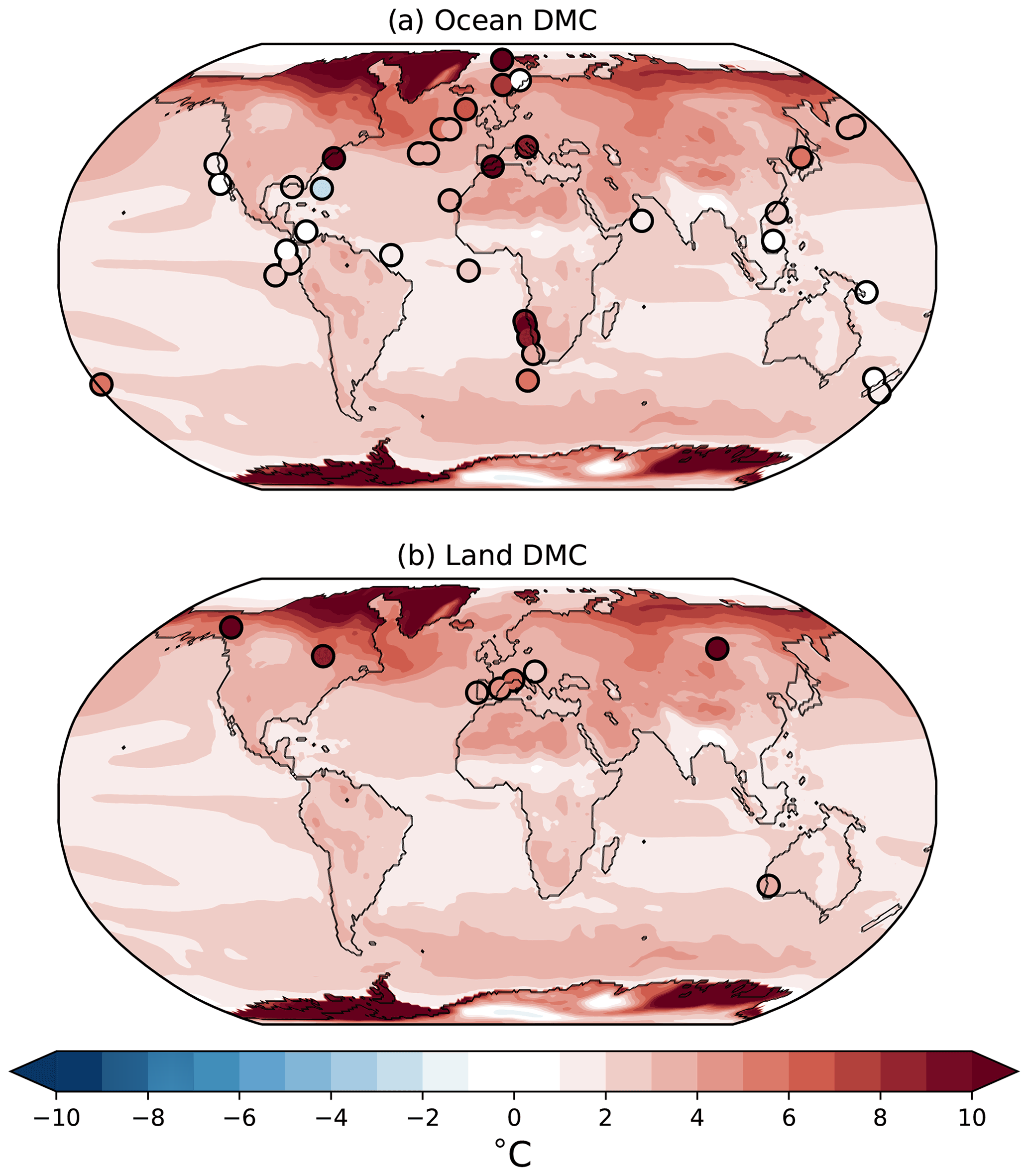
Figure 1The background colours are multi-model mean results from PlioMIP2 (Haywood et al., 2020). (a) The ocean site data SST anomaly is the difference between the McClymont et al. (2020) dataset and years 1870–1899 of the NOAA Extended Reconstructed Sea Surface Temperature (ERSST) version 5 dataset (Huang et al., 2017). (b) The terrestrial data SAT anomaly is the difference between the KM5c terrestrial dataset and the CRU reanalysis data (CRU TS v 4.04; Harris et al., 2020) averaged over the period 1901–1930.
Despite the limited data, Fig. 1b suggests that the models are unable to accurately simulate terrestrial polar amplification. If this is true it could be very concerning when simulating future climate change. It is therefore crucial to improve our understanding of why models and data do not agree at terrestrial high latitudes.
Although the ocean model–data discrepancy seen in PlioMIP1 has been reduced in PlioMIP2 (Haywood et al., 2020; McClymont et al., 2020), the terrestrial model–data discrepancy remains. In this paper we will analyse the terrestrial DMC in more detail. We will show that the model–data discrepancy is mostly confined to the high-latitude winter temperatures; temperatures from the data are greatly in excess of those from the models. This winter temperature discrepancy will be termed the “warm winter paradox”. We will consider several possible reasons for the warm winter paradox including: model boundary condition and structural uncertainty, proxy data not being strongly constrained by winter temperatures, uncertainties in data reconstruction methods, uncertainties in proxy dating, and the fact that in some parts of the world the Pliocene climate is outside the modern sample. We will also show that uncertainties in summer temperatures are very different from those in winter temperatures and that a summer DMC is likely to lead to more accurate results.
The layout of the paper is as follows. Section 2 will describe the modelling and methods used. Section 3 will present a DMC focusing on both the annual mean and seasonal temperatures. Section 4 will discuss possible reasons for the warm winter paradox. A discussion of the results and conclusions will be presented in Sect. 5.
2.1 Climate modelling
This paper makes use of two sets of modelling simulations to represent the mPWP. The first set is the model results from PlioMIP2, and the second is a set of simulations run with the HadCM3 climate model to assess uncertainties caused by orbital forcing. These are described below.
2.1.1 PlioMIP2 core experiments
The PlioMIP2 ensemble (Haywood et al., 2020) is the largest consistent set of mPWP model simulations to date. All modelling groups participating in PlioMIP2 were required to run a preindustrial experiment and a core mPWP experiment, which was intended to represent the KM5c time slice (3.205 Ma). Boundary conditions for the core mPWP experiment included CO2 of 400 ppmv (which is within the range obtained by de la Vega et al., 2020) and a modern orbit. The land–sea mask, topography, bathymetry, vegetation, soils, lakes, and land ice cover were obtained from the latest iteration of PRISM (PRISM4; Dowsett et al., 2016). It must be noted that the boundary conditions were not implemented identically in all of the PlioMIP2 models, although there is substantial commonality. See papers referenced in Table 1 for details of how each model implemented the boundary conditions.
Feng et al. (2020)Baatsen et al. (2021)Chandan and Peltier (2017)Feng et al. (2020)Feng et al. (2020)Stepanek et al. (2020)Zheng et al. (2019)Hunter et al. (2019)Williams et al. (2021)Tan et al. (2020)Tan et al. (2020)Chan and Abe-Ouchi (2020)Kamae et al. (2016)Li et al. (2020)Li et al. (2020)Table 1Models participating in PlioMIP2 used in this study.

NA: not available.
2.1.2 HadCM3 orbital sensitivity experiments
The KM5c time slice had an orbit very close to modern (Haywood et al., 2013), and hence all PlioMIP2 experiments were run with a modern orbit. Over land, it is difficult to obtain data with orbital temporal precision, and in order for a DMC to even be possible it is necessary to utilize data from outside the KM5c time slice and sometimes even outside the mPWP. It is reasonable to utilize such data, provided that one is aware that this will lead to errors in the DMC. Close to the KM5c time slice these errors are mainly due to orbital configuration, and hence we include orbital uncertainties in the modelled climate when comparing with terrestrial palaeodata. Data that are further away from KM5c, such as from the early Pliocene, can also be compared with the PlioMIP2 models, provided that one is aware of the low confidence in the results due to errors in other modelled boundary conditions (e.g. CO2, ice sheets) which are difficult to quantify.
The PlioMIP2 experimental design did not include orbital sensitivity experiments. We therefore assess orbital uncertainty by including a number of sensitivity experiments run with a single model, HadCM3 (Gordon et al., 2000). Table 2 shows the top-of-the-atmosphere (TOA) insolation for specified times within the period 2.9 to 3.3 Ma. The first block shows the most extreme TOA insolation for January and July at 65∘ N, and the second block shows the most extreme TOA insolation for January and July at 56∘ N. The third block shows the HadCM3 modelling sensitivity experiments that we used in this paper along with their time slice and TOA insolation. It is seen that the orbits we use here cover relatively extreme orbits for the latitudes of interest. The orbits representing G17 (2.950 Ma), K1 (3.060 Ma), and KM3 (3.155 Ma) have already been discussed by Prescott et al. (2014). They all show high July TOA insolation, and K1 also shows high January TOA insolation at 65∘ N. Here, we use an additional orbit, 3.037 Ma, which maximizes January TOA insolation at 56∘ N, and this orbit shows a smaller TOA insolation in July than the others used. We choose orbits which are designed to produce high TOA insolation, as these will produce warmer temperatures and would be expected to reduce the model–data disagreement seen in Fig. 1.
Table 2TOA insolation at various times in the mPWP. The TOA insolation for each orbit was obtained using Laskar et al. (2004). Values in bold highlight the maximum and minimum insolation in each column.

2.2 Vegetation modelling
We simulate mPWP vegetation by using the PlioMIP2 climate to drive the BIOME4 mechanistic global vegetation model (Kaplan, 2001). BIOME4 has been used in many previous studies of the mPWP (e.g. Salzmann et al., 2008; Pound et al., 2014; Prescott et al., 2018), and it predicts the distribution of 28 global biomes based on the monthly means of temperature, precipitation, cloudiness, and absolute minimum temperature.
There are two ways to run the BIOME4 model. These are (a) absolute mode or (b) anomaly mode. For the absolute mode, BIOME4 is driven by direct climate model outputs for the period of interest. The anomaly mode accounts for known climate model biases that occur in the model's modern simulation and are likely to propagate through to other time periods. In anomaly mode climate inputs to BIOME4 are obtained by calculating the modelled climate anomaly from the preindustrial and adding this onto modern observations as follows:
where x is one of the BIOME4 inputs (temperature, precipitation, cloudiness, absolute minimum temperature), input denotes a parameter input to BIOME4, model denotes a simulated value from the multi-model mean, and obs is a modern dataset, which was based on observations and created for BIOME4, as described by Kaplan et al. (2003).
In this paper we will use the anomaly mode because this gives a more detailed representation of possible biomes, particularly at small spatial scales. However, in the Supplement (Fig. S1) we will also show results from the absolute mode to highlight that, for the mPWP, large-scale features of biomes are not dependent on the methodology used.
3.1 mPWP mean annual temperature
There are eight palaeovegetation data sites that are compared with PlioMIP2 model results in Fig. 1b. Figure 2 shows the DMC for each of these sites with values reported in Table S1 in the Supplement.
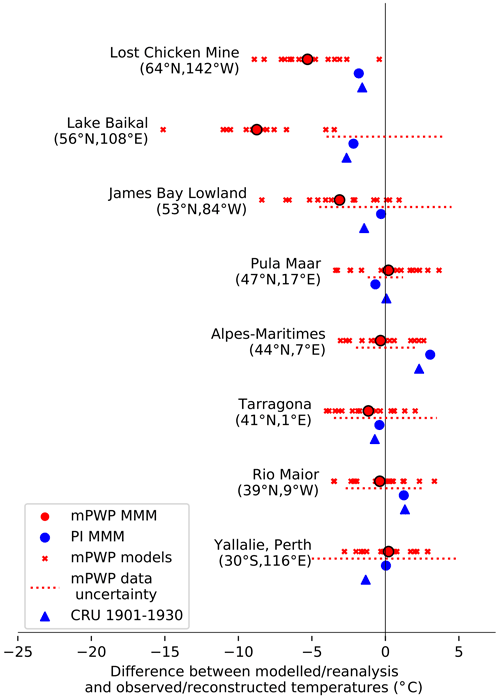
Figure 2Blue circles shows the difference between MMM preindustrial MAT and modern observations at the site. The blue triangle shows the difference between the CRU MAT for years 1901–1930 and the modern observations at the site, representing an estimate of the error caused by comparing a single modern data point to a preindustrial model grid box. The red circle shows the difference between MMM mPWP MAT and the MAT reconstructed from the proxy; red crosses show the anomalies for the individual models. The red dotted line shows the uncertainty in the data reconstruction (where available).
In Fig. 2 the blue circles show the difference between the multi-model mean (MMM) PI mean annual temperature (MAT) and the modern observed MAT at the data site. The blue triangle shows the anomaly between the modern observations and the CRU reanalysis data and is intended to represent the expected error bar due to comparing modern MAT at a site to a grid-box-sized area for the preindustrial. It is seen that the PI MMM MAT and the CRU reanalysis data have a similar anomaly from the point-based observations, suggesting that there is no inherent model bias at these locations.
Red symbols in Fig. 2 show the difference between the mPWP PlioMIP2 simulations and the MAT obtained from the palaeovegetation-based climate reconstruction. The red circle is the MMM and the small crosses show results from the 17 individual models. Error bars on the reconstructed temperatures due to the combined bioclimatic and temporal variability are shown by the red dotted lines (where available).
Figure 2 shows very good model–data agreement for the mPWP at the five sites between 47∘ N and 30∘ S. The higher-latitude sites (at 64, 56, and 53∘ N) do not show good model–data agreement. Instead the mPWP temperature suggested by the data is substantially higher than the MMM. Although no definitive conclusions can be drawn from such a small number of data points, it appears that the models have more difficulty in reproducing the data at higher latitudes than at lower latitudes. This was also shown by Salzmann et al. (2013).
3.2 Seasonal temperatures
We now consider whether the mPWP model–data disagreement seen at high latitudes is uniform throughout the year or whether it occurs preferentially in certain seasons. Figure 3 and Table S2 show the PlioMIP2 model results compared with Pliocene palaeovegetation-derived temperatures for the warmest and coldest months of the year. More details about the sites used for this comparison can be found in Table 3. Ideally this comparison would be for the KM5c time slice only; however, we incorporate additional Pliocene data because only two sites can be dated close to KM5c.
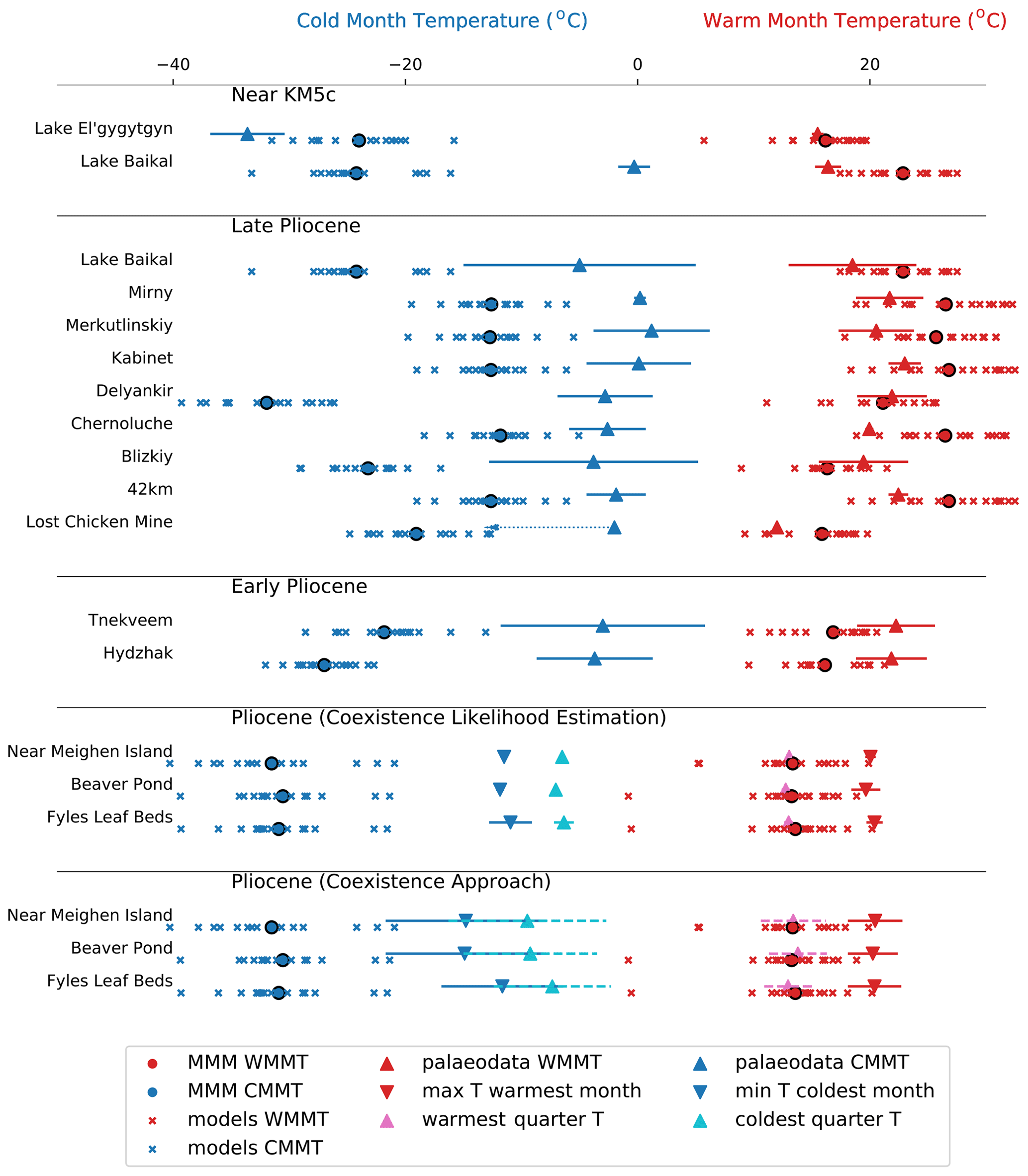
Figure 3Data–model comparison for the cold month mean temperature (CMMT; blue) and the warm month mean temperature (WMMT; red). Triangles show temperatures from proxy data with published uncertainties (where available). The Pliocene CMMT at Lost Chicken Mine was reported as “less than −2 ∘C but not nearly as cold as the modern”, and this is represented by the dotted line and arrow. The location of Meighen Island (80∘ N, 99∘ W) was an oceanic grid box in most models, and hence Meighen Island data have been compared to a nearby land grid box. Model data are WMMT or CMMT and are shown by circles (MMM) or small crosses (individual models). Additional metadata are in Table 3.
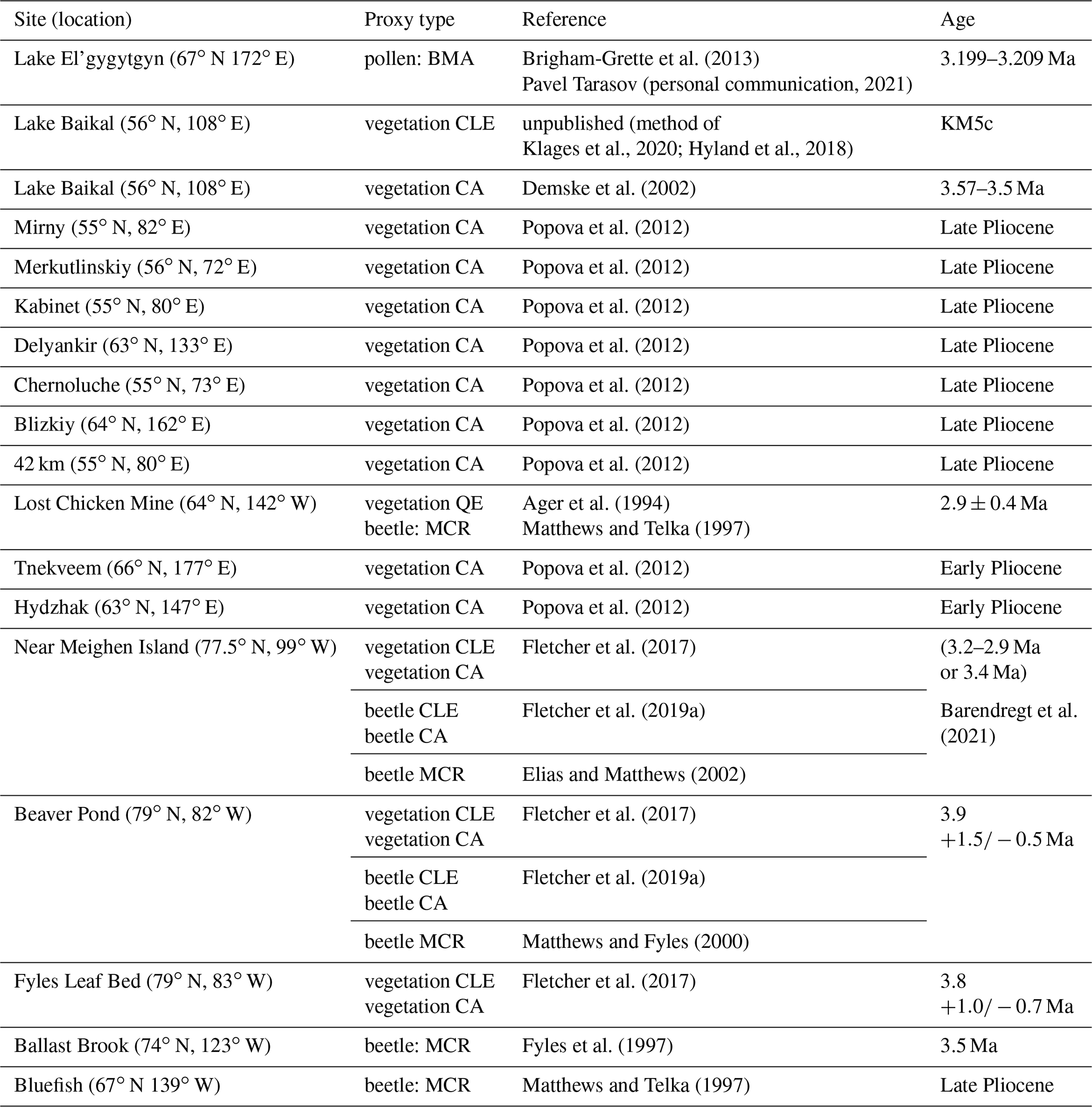
Table 3Metadata for the DMC in Figs. 3 and 4. BMA – best modern analogue (Overpeck et al., 1985), CA – coexistence approach based on Mosbrugger and Utescher (1997), CLE – coexistence likelihood estimation, QE – qualitative estimates using modern analogues, MCR – mutual climatic range.
For the KM5c DMC, the PlioMIP2 MMM agrees very well with the warm month temperature at Lake El'gygytgyn (data: 15–16 ∘C, MMM: 16.2 ∘C), although the warm month temperature MMM is ∼6 ∘C warmer than the data at Lake Baikal (data: 15.2–17.5 ∘C, MMM: 22.8 ∘C). For the cold month temperature, there is a larger discrepancy between the MMM and the data. The MMM cold month temperature is ∼6 ∘C warmer than that obtained from data at Lake El'gygytgyn and ∼23 ∘C colder than that obtained from data at Lake Baikal. At Lake Baikal even the warmest model (CESM2) simulated the cold month temperature ∼15 ∘C too cold. The data suggest that the KM5c cold month temperature at Lake El'gygytgyn was >30 ∘C cooler than at Lake Baikal; however, none of the models show this: all models suggest that the two sites differ in temperature by less than 6 ∘C.
The second block in Fig. 3 shows how the PlioMIP2 models compare with other late Pliocene data. This DMC has the caveat that the modelled data represent a different temporal slice to what has been reconstructed. Because of this temporal mismatch we would expect some model–data disagreement; however, we would highlight large model–data discrepancies as problematic. For example, at Lake Baikal we have two reconstructed temperatures: one near KM5c and the other dated as 3.57–3.5 Ma (Demske et al., 2002). Although the reconstructed temperatures at these two dates differ, this difference is relatively small compared to the large model–data discord that occurs at this site. This suggests that accounting for dating uncertainties would not be sufficient to explain the very large model–data mismatches for the cold month temperature for the late Pliocene Lake Baikal site.
Further late Pliocene climatic data from Russia were obtained by Popova et al. (2012) and are compared with model results in Fig. 3 (sites: Mirny, Merkutlinskiy, Kabinet, Delyankir, Chernoluche, Blizkiy, and 42 km). These sites show similar reconstructed temperatures as those at Lake Baikal and corroborate a strong model–data discord for the coldest month. Additional data for the early Pliocene (sites Tnekveem and Hydzhak) also show the same pattern; however, we do note that confidence in the DMC comparison is lower for the early Pliocene sites.
North American sites are also included in Fig. 3 at Lost Chicken Mine and the Canadian Arctic sites of Meighen Island, Beaver Pond, and Fyles Leaf Bed. The Canadian Arctic sites have temperatures reconstructed using two different methods: coexistence likelihood estimation (CRACLE; Harbert and Nixon, 2015) and an open-data method based on the coexistence approach (Fletcher et al., 2017; Mosbrugger and Utescher, 1997). Regardless of the exact dating, location, or reconstruction method, the DMC over North America follows the same pattern as that seen over northern Asia: the modelled temperatures are far too cold for the coldest month, and the model–data agreement is much better for the warmest month. Differences in location, proxy age, or reconstruction method can affect the temperature but are not large enough to affect the general conclusion of cold month model–data discord.
Other proxies which provide summer temperature at the Beaver Pond site agree with warm season temperatures derived from the palaeovegetation and are close to the warm month temperature from the models. These are (1) average mean summer temperatures of 15.4±0.8 ∘C derived from branched glycerol dialkyl glycerol tetraethers (Fletcher et al., 2019b), (2) average growing season temperature of (a) 14.2±1.3 ∘C derived from δ18O values of cellulose and aragonitic freshwater molluscs, and (b) 10.2±1.4 ∘C derived by applying carbonate “clumped isotope” thermometry to mollusc shells (Csank et al., 2011). For context, the median modelled summer (JJA) temperature at the Beaver Pond site is 10.2 ∘C with a 20th–80th percentile range of 7.8–14.0 ∘C.
Other proxies which provide annual mean temperature at the Beaver Pond site agree less well with the annual mean temperatures from the models. In addition to coexistence of palaeovegetation-derived temperatures ( ∘C), Ballantyne et al. (2010) derived annual mean temperatures using oxygen isotopes and annual tree ring width ( ∘C) as well as bacterial tetraether composition in paleosols ( ∘C). These temperatures are much warmer than suggested by the models (median temperature −11.4 ∘C).
In addition to the above proxies, the literature contains reconstructions of both warm month and cold month Pliocene temperatures from beetle assemblages over the high latitudes of North America. However, the cold season temperatures are less well constrained than warm month temperatures (e.g. Elias et al., 1996; Elias and Matthews, 2002; Huppert and Solow, 2004). This may mean that the cold season temperature derived from beetles might reflect the modern seasonal range of temperature in the calibration dataset rather than the Pliocene cold season (Fletcher et al., 2019a).
Figure 4 compares the PlioMIP2 models to the North American beetle assemblage data and shows good model–data agreement for the warm month temperature. Unlike the DMC for the palaeovegetation proxies, the MMM agrees reasonably well with the cold month temperature reconstructed from beetle data, particularly that derived using the mutual climate range method. However, this model–data agreement may be due to large error bars on both models and beetle data and may be due to neither of them being able to produce large enough anomalies from the modern climate (Fletcher et al., 2019a). It is unclear what causes this large disagreement on winter temperatures obtained from various sources, and we will refer to this contradiction as the warm winter paradox. Resolving this warm winter paradox is essential if we are to bring models into line with the data and understand the true nature of the Pliocene cold season climate.
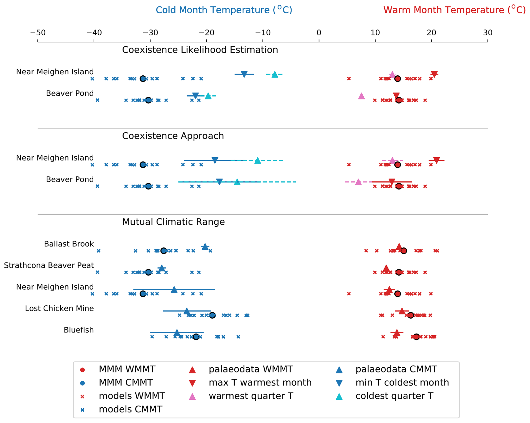
Figure 4Data–model comparison for the cold month mean temperature (CMMT: blue symbols) and the warm month mean temperature (WMMT: red symbols) for the Pliocene. Triangles show temperatures from beetle assemblage proxy data, which were obtained using various methods with published uncertainties (where available). Model data are shown by circles (MMM) or small crosses (individual models). The location of Meighen Island (80∘ N, 99∘ W) was an oceanic grid box in most models, and hence Meighen Island data have been compared to a nearby land grid box. Additional metadata for this figure are in Table 3.
3.3 Biomes
Figure 5a shows the mPWP high-northern-latitude biome reconstruction (Salzmann et al., 2008). This can be compared with Fig. 5c, which shows the biomes simulated at these locations using the MMM mPWP climate and BIOME4. The modelled biome agrees with the reconstructed biome at 14 of the 30 sites. Sites where the model suggests a different biome to that reconstructed are shown in Fig. 5d. For most of the sites where the modelled biome is different to the reconstruction (particularly over North America), the reconstructed biome can be modelled at a nearby location (see Fig. 5b), suggesting that some discrepancies are due to small spatial errors. Over Europe, the warm mixed forest in the model extends too far to the east and the MMM does not reproduce the extent of the cool mixed forests seen in the data. However, it is quite easy to simulate cool mixed forest in this region with only minor parameter changes to the BIOME4 model (not shown), suggesting that models and data are “close” in this region.
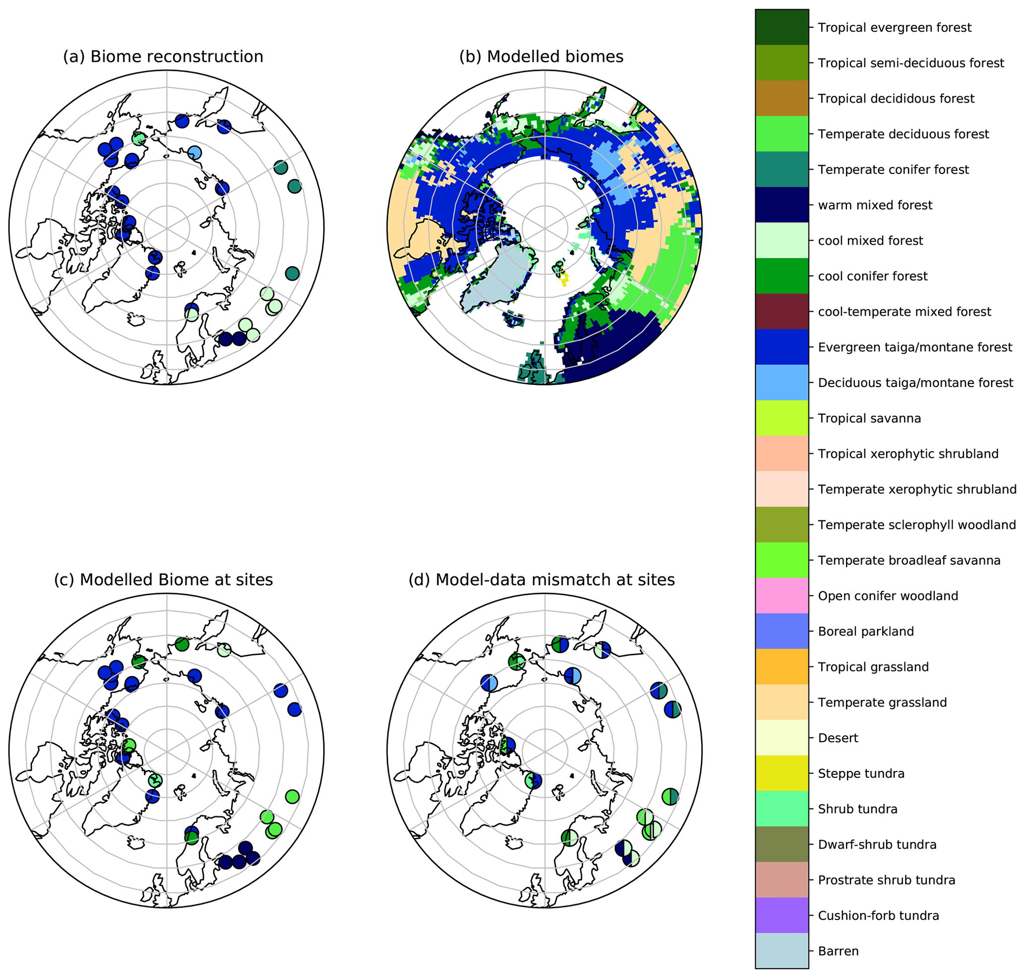
Figure 5(a) The reconstructed biomes from Salzmann et al. (2008). (b) The modelled biomes obtained by using the PlioMIP2 MMM to drive the BIOME4 model. (c) The modelled biomes in (b) at the locations where data are available. (d) Locations where the reconstructed biomes do not match the modelled biome. The modelled biome is the left of the semicircle, and the reconstructed biome is to the right of the semicircle.
A notable region of data–model mismatch is in central Asia. Here, the reconstructed biome is “temperate conifer forest” and the model simulates “evergreen taiga”. BIOME4 can only simulate temperate conifer forest when the cold month temperature is above −2 ∘C, a condition that is not provided by any of the PlioMIP2 models. The biome data–model mismatch in this region is not easily resolved and is due to the warm winter paradox (i.e. data suggesting warmer winters than can be modelled). However, in North America and Europe the warm winter paradox does not prevent BIOME4 from simulating the correct vegetation biome.
4.1 Could proxy dating uncertainties help resolve the warm winter paradox?
Haywood et al. (2013) suggested that the mismatch between models and data for PlioMIP1 might be caused by a comparison between model results representing a short time slice and data that represented the ∼300 000 years of the mPWP. Moving to the KM5c time slice for both models and data in PlioMIP2 has addressed this methodological error, and there is an improvement in model–data agreement for ocean proxies (Haywood et al., 2020; McClymont et al., 2020).
A terrestrial DMC for the KM5c time slice is problematic because there are very few terrestrial data with suitable temporal precision, and it was necessary to incorporate some data from outside the time slice. It is therefore important to check whether the warm winter paradox could be reduced (or even eliminated) by accounting for temporal model–data mismatches.
Proxy dating uncertainties have previously been explored with modelling sensitivity experiments using different orbital configurations. These were found to show better data–model agreement in the annual mean temperature at high latitudes (e.g. Feng et al., 2017; Hill, 2015; Howell et al., 2016). It is relatively easy to increase the annual mean temperature at high latitudes by changing the orbital configuration (e.g. Prescott et al., 2014), and it is tempting to use this as a partial solution as to why models and data do not agree. However, since the model–data mismatch occurs in the winter season, any orbital solution must increase the cold month temperature and have a smaller effect on the warm month temperature.
Here we use the HadCM3 model to assess how different orbital configurations in the mPWP would change the warm month and cold month temperatures. The orbital configurations we include are shown in Table 2. Although the list is not exhaustive, it includes enough of the extreme orbital configurations to allow an assessment of whether orbit is likely to prove important for resolving the warm winter paradox.
Figure 6a shows the difference between the model and data for the cold month temperature for sites dated as KM5c or late Pliocene. The HadCM3 simulation representing the KM5c time slice is shown by the orange square, while the triangles show the HadCM3 simulations for other time slices considered. For context, the red circles show the KM5c simulation for other PlioMIP2 models. As expected, the simulation which had the largest January insolation (3.053 Ma) produced the warmest cold month temperatures. However, the cold month temperature is more sensitive to which model is used than the exact orbital configuration. This suggests that structural model uncertainties are a more likely contributor to the warm winter paradox than uncertainties in the exact time slice that is to be compared with the data.
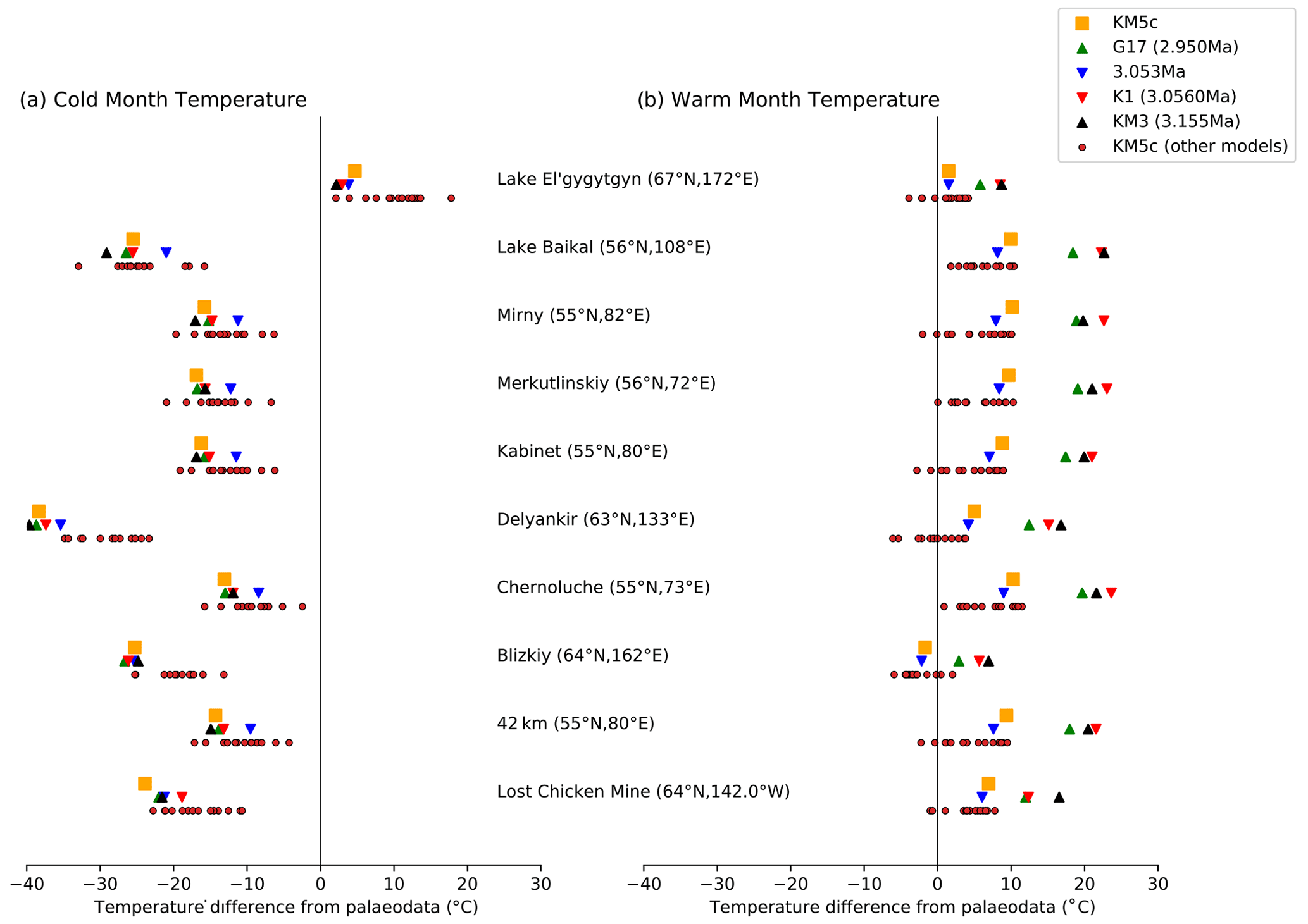
Figure 6The difference between the modelled temperature and the palaeodata. The palaeodata are dated to KM5c for Lake Baikal and Lake El'gygytgyn and are dated to the late Pliocene for other sites. HadCM3 simulations with a range of different orbital configurations are shown by the square and triangles. The KM5c simulation for other models is shown by the circles.
Figure 6b shows that the orbital configuration chosen can strongly affect the warm month temperature. This is unsurprising because the summer insolation is much more variable than the winter insolation (Table 2). If we had a “warm summer paradox”, then dating errors could be an important part of the solution. Figure 6 highlights the major shortcoming of using “warm” orbital configurations to improve model–data agreement for the annual mean temperature. In the annual mean (Fig. S2) both the K1 and KM3 simulations can predict higher temperatures than KM5c (e.g. at Lost Chicken Mine) and show the best agreement with the annual mean temperature reconstructions. However, neither K1 or KM3 produces a good representation of cold month or warm month temperatures. In addition, neither of these simulations is able to simulate realistic Pliocene biomes (Prescott et al., 2018). This highlights that a DMC for annual mean temperatures is insufficient for determining the extent of model–data agreement.
This subsection asked the following question: could proxy dating uncertainties help resolve the warm winter paradox? If we assume that dating uncertainties can be quantified by assessing the most extreme orbital configurations in the mPWP, then the answer is that proxy dating uncertainties are unimportant for the winter season. However, the orbital configuration is not the only model boundary condition that would change as we progress through all the time slices that make up the Pliocene. Other boundary conditions would include changes in trace gas, ice sheet extent, vegetation distribution, ocean gateways, and associated feedbacks. Sensitivity tests using different values of CO2 (not shown) suggest that changing CO2 would not lead to preferential warming in a particular season. It remains to be explored whether changing other modelled boundary conditions (e.g. ice sheets) could have a preferential effect on warming the winter season. However, the PlioMIP2 simulations only include a small ice sheet over Greenland, and hence there is limited scope for reducing ice sheets further in the Northern Hemisphere.
4.2 Could local climate effects help explain the warm winter paradox? (a case study of Lake Baikal)
Figure 3 shows very different results for the two sites dated near KM5c, with the PlioMIP2 models simulating the temperature better at Lake El'gygytgyn than at Lake Baikal. Here we consider the DMC at Lake Baikal in more detail to assess why this might be the case.
It is known that large bodies of water retain heat longer than the land; hence, the climate around Lake Baikal is much milder than the rest of southern Siberia. However, most models do not accurately simulate the climate-stabilizing effects of the lake and their prediction of climate at this location is more representative of the wider region than the local site.
Meteorological observations for three sites near Lake Baikal are shown in Table 4. Nizhneangarsk is on the northern edge of Lake Baikal, while Zhigalovo is 4∘ to the west and Kalakan is 7∘ to the east. Even though Nizhneangarsk lies between the other two sites, the large heat capacity of Lake Baikal means that it has warmer annual mean temperature, warmer January temperature, and colder July temperature. To quantitatively estimate how much the lake will stabilize the temperature we compare observations at Nizhneangarsk with the temperature interpolated onto the Nizhneangarsk location from observations at Zhigalovo and Kalakan (see Table 4). Comparing this interpolated temperature with that recorded suggests that the presence of the lake increases the annual mean temperature by 1.8 ∘C, increases the January temperature by 7.8 ∘C, and cools the July temperature by 2 ∘C. Assuming that Lake Baikal affected the mPWP climate in an analogous way, the model results can be corrected by this amount. This correction reduces the mPWP annual mean data–model discrepancy at this site from 8.5 to 6.9 ∘C, the warm month temperature data–model discrepancy from 6 to 4 ∘C, and the cold month data–model discrepancy from 23 to 15 ∘C. This correction is not sufficient to allow model–data agreement for the Pliocene winter. However, it does improve model–data agreement and will be one of a number of factors that need consideration in the Pliocene DMC.
Table 4Station temperature data near Lake Baikal averaged over 1950–1970.
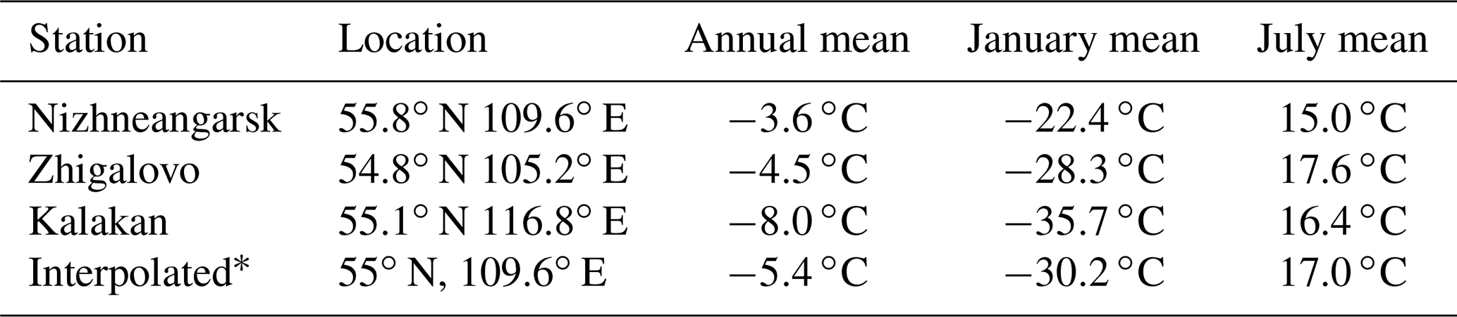
* Interpolated data are from Kalakan and Zhigalovo.
A small caveat to this approach is that some models already account for the climate-stabilizing effects of the lake. For example, CESM2 and GISS2.1G contain a lake component, and both include a realistic representation of lakes in their preindustrial and mPWP simulation. These models do not need correcting to account for the climate-stabilizing effects of the lake, and applying such a correction would reduce agreement with observations for the modern climate. Ultimately it is a choice for individual modelling groups as to whether their model output needs correcting to account for microclimate effects at a specific location. In our study we suggest that the MMM temperatures at Lake Baikal requires a “lake” correction because it is required for the majority of the PlioMIP2 models.
4.3 Can other uncertainties in reconstructed temperatures help explain the warm winter paradox?
4.3.1 Vegetation proxies may not be strongly related to the cold month temperature
The cold month temperatures from the PlioMIP2 models are lower than reconstructed from data. Over northern Asia this leads to a mismatch between reconstructed biomes and biomes simulated by BIOME4. However, both the cold month temperature reconstructions and the BIOME4 model assume that the cold month temperature is a strong constraint on the distribution of tree species and that the limits on the range of trees can be determined using correlations from the modern climate. In fact, these assumptions may not hold. A case study from Korner et al. (2016) found that for temperate tree species, low-temperature extremes in winter (when the species were dormant) have very little relationship to range limits and that tree species could tolerate much cooler winter temperatures than those that are currently experienced. Spring temperature was found to be far more important for determining whether a species can survive and reproduce, and growing season temperature is also important. This suggests that the uncertainties regarding winter temperatures may be much larger than is sometimes reported.
4.3.2 Possible errors in reconstruction methods
Palaeoclimate reconstruction methods can be used to reconstruct modern climate. These modern reconstructions can be compared to modern observations to provide error bars on the method. Following this approach, Harbert and Nixon (2015) found that the average error for the MAT reconstructed using the CRACLE method1 was 1.3–1.4 ∘C, which compared well with errors of 1.8 ∘C for CLAMP and 2 ∘C for leaf margin analysis. None of these errors are large enough to notably contribute to the data–model mismatch found for the Pliocene. However, these errors are global averages and do not appear uniformly over the globe. Harbert and Baryiames (2020, their Fig. 2) show that the error in reconstructing the minimum temperature of the coldest month appears larger at cold temperatures than the average error over the globe. For example, sites with minimum temperature below −20 ∘C appear to have a clear warm bias, which also occurs in the mean annual temperature. No clear bias is apparent when reconstructing the maximum temperature of the warmest month. If this warm bias in the minimum temperature is robust and also occurs in the Pliocene temperature reconstruction, it could contribute to the model–data discord seen in Figs. 2 and 3.
4.3.3 Different proxies suggest different cold month temperatures
We note from Figs. 3 and 4 that there are differences in the temperature reconstructions from different proxies. It is beyond the scope of this paper to compare and contrast proxy methods, and this subject is covered in other papers (e.g. Harbert and Nixon, 2015; Fletcher et al., 2019a). However, two things are of note. Firstly, the only two sites that are close to KM5c in Fig. 3, Lake Baikal and Lake El'gygytgyn, have similar warm month temperature reconstructions but suggest cold month temperatures that differ by over 30 ∘C, a feature that does not occur in any of the models or in modern observational data. Could some of this difference between the two sites be related to the different methodologies used for temperature reconstruction (Table 3)? Secondly, differences between proxy-reconstructed temperatures for the Pliocene are often larger than published error bars (or may result from some published ranges not including error bars). For example, the cold month mean temperature from the coexistence likelihood estimation provides a warmer temperature than the coexistence approach, which provides a warmer temperature than the mutual climatic range method for beetle assemblages (Figs. 3 and 4). For the warm month mean temperature all approaches yield similar temperatures. Note that here we are not suggesting that one reconstruction of the cold month mean temperature is better than another; instead we are pointing out that the cold month temperature from proxy data appears to be subject to greater uncertainty than the warm month temperatures.
4.4 Could modelling errors be responsible for the warm winter paradox?
Models are, by their nature, an imperfect representation of reality and all models have errors, even for the preindustrial for which boundary conditions are well known and for which some model parameters have been chosen based on their ability to produce a realistic climate. Pliocene simulations use the same model parameters that have been optimized for the modern climate and also have less well-constrained boundary conditions. Hence, the simulated Pliocene climate contains more uncertainties than the corresponding preindustrial simulations.
Figure 3 shows that across the PlioMIP2 ensemble there is large variation in the simulated cold month mean temperature (up to ∼20 ∘C). This large range is from a suite of models that have been run with very similar boundary conditions (orbit, CO2, ice sheets), so the model spread is likely due to inherent model structure. The PlioMIP2 models have equilibrium climate sensitivities2 between 2.3 and 5.2 ∘C, which covers the range suggested by IPCC, and hence the ensemble response to CO2 forcing is likely reasonable. However, the modelled response to the full Pliocene boundary condition changes (e.g. ice sheets and orography) is less constrained by other sources. There may also be some important forcings (e.g. methane; Hopcroft et al., 2020) that have not been included in the PlioMIP2 simulations and some important feedbacks, for example fire (Fletcher et al., 2019b) and chemistry (Unger and Yue, 2014), that are not included.
Clouds and convection feedbacks are subject to uncertainties and could lead to errors in Pliocene simulations. Abbot and Tziperman (2008) used a single column model to show that deep atmospheric convection might occur during winter in ice-free high-latitude oceans and could increase high-latitude winter temperatures by ∼50 ∘C. However, this feedback did not occur in any of the PlioMIP2 models despite January Arctic sea ice extent being reduced by up to 76 % (de Nooijer et al., 2020).
Another potential source of model error might be that the PlioMIP2 models do not have high enough resolution to fully resolve the processes occurring in the Pliocene. For example, Arnold et al. (2014) showed that modelling a high-CO2 world with a cloud-permitting model led to greater Arctic cloud cover and sea ice loss than if convection were parameterized. However, these changes had relatively minor effects on Arctic temperatures.
Pope et al. (2011) considered the uncertainty that could result from incorrect tuning of the model parameters in the HadCM3 model by running a Pliocene perturbed physics ensemble which varied uncertain model parameters (within reasonable bounds). They showed that the effect of using model parameters designed to produce a high-sensitivity climate could be substantial (approximately 2–5 ∘C of warming in the Pliocene over the high-latitude continents). However, they presented their results for the annual mean temperature only, so we currently do not know how this increase would manifest seasonally. They also noted that when this “high-sensitivity” climate was used to drive BIOME4 then the biome distribution did not agree with reconstructions or the biome distribution simulated from the control climate.
It is likely that as models develop there will be future refinements to the Pliocene model simulations, and this could provide part of the solution to the warm winter paradox. However, the current set of PlioMIP2 experiments provides good agreement with ocean data (McClymont et al., 2020; Haywood et al., 2020), so the potential for model refinements is subject to ocean data constraints and may not change as much as is needed to fully agree with the cold month terrestrial temperature data.
4.5 Could a geographical shift in biome boundaries explain the warm winter paradox?
Figure 7 shows that in the Pliocene the high-latitude forests were further poleward than they were in the preindustrial climate. This is logical because in a warmer climate vegetation would be able to inhabit regions that are too cold today. However, this does not mean that the climate experienced by a biome in the Pliocene will be exactly the same as the climate experienced by that biome today.
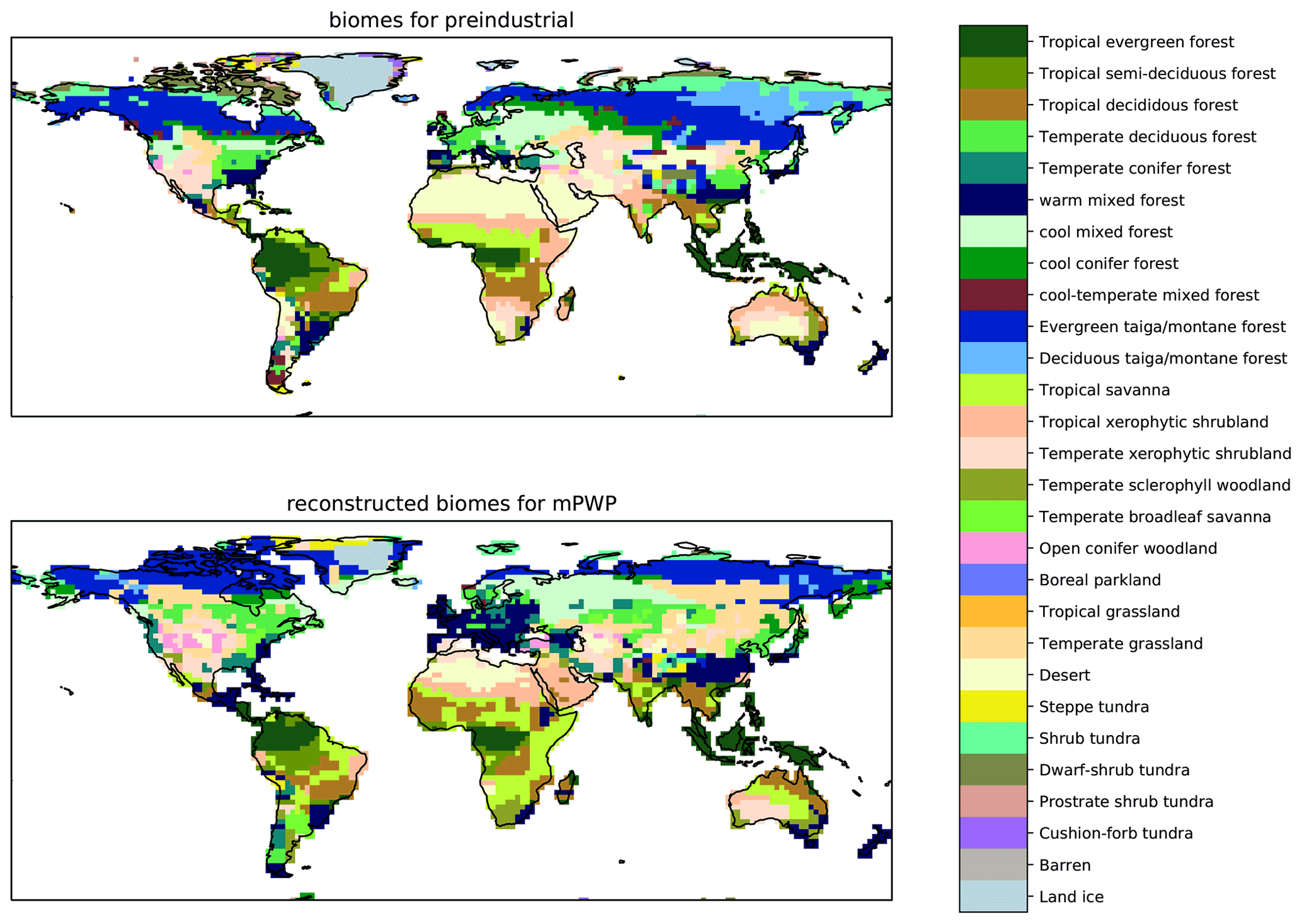
Figure 7A comparison of modern biomes with the reconstructed biomes for the mPWP (Salzmann et al., 2008).
Figure 8 shows the incoming solar insolation at the top of the atmosphere for each month and latitude. For clarity this has been normalized by the incoming solar radiation at 55∘ N. We see that in May–June–July the insolation at all latitudes shown is similar to the insolation at 55∘ N, while in other months (particularly the winter) the insolation (relative to that at 55∘ N) decreases dramatically as we move to higher latitudes. Because KM5c has a nearly modern orbit, Fig. 8 applies to both KM5c and the modern climate and is one of the most certain features of the KM5c world.
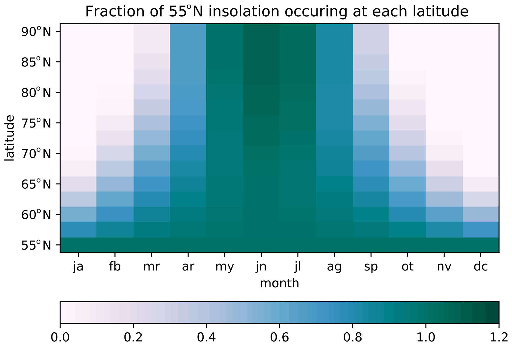
Figure 8TOA insolation by latitude and month. This has been normalized by dividing the insolation for a latitude and month by the insolation for that month at 55∘ N.
We can be confident that if a plant species occupied a higher-latitude niche at KM5c than it does today then the amount of incoming solar insolation it experienced would vary more throughout the year. As an example, Fletcher et al. (2019b) showed that the Pliocene floral assemblage at Beaver Pond (∼79∘ N) most closely resembles modern vegetation found in northern North America, particularly at the Eastern Margin, the Western Margin, and Fennoscandia. All of these locations are at latitudes <70∘ N, and some are at latitudes <50∘ N. It is seen in Fig. 8 that these lower-latitude analogues will have a much less extreme seasonal cycle of insolation than Beaver Pond. Of course, climate feedbacks at the Pliocene Beaver Pond site could counteract the seasonal cycle in insolation and allow the seasonal temperature cycle to become similar to the modern climate at a lower latitude. However, it is likely that this would not be the case for every location over the globe, and some middle- to high-latitude ecosystems in the mid-Pliocene could experience environmental conditions outside the modern sample. This would lead to uncertainties in climate reconstruction methods that utilize information from the modern distribution of plants to determine past climates. Any such uncertainties would increase error bars on winter temperatures because plant distributions are more strongly constrained by spring and summer temperatures (Korner et al., 2016). Furthermore, the error bars would likely be skewed towards colder temperatures because winter insolation becomes strongly reduced as we move to higher latitudes. We therefore highlight the geographical shift in biome boundaries and the potential for a non-analogue climate as another possible contributor to the warm winter paradox.
The latest iteration of the Pliocene Modelling Intercomparison Project (PlioMIP2) produces temperatures that agree very well with proxy data for oceans, the tropical land surface, and the high-latitude land surface warm month temperature. The high-latitude cold month mean temperature, however, shows large model–data disagreement. The proxy data suggest very high temperatures that the models are unable to replicate. We term this the “warm winter paradox”.
This cold month, high-latitude, terrestrial data–model discord is not unique to the Pliocene. For the Holocene, Mauri et al. (2015) noted that their “climate reconstruction suggests warming in Europe during the mid-Holocene was greater in winter than in summer, an apparent paradox that is not consistent with current climate model simulations and traditional interpretations of Milankovitch theory”. For the Last Glacial Maximum (LGM), Kageyama et al. (2021) showed that none of the models analysed could simulate the amplitude of the reconstructed winter cooling over western Europe. For older, greenhouse climates in the Mesozoic and early Cenozoic there has been a long-standing “equable climate problem” (e.g. Greenwood and Wing, 1995; Huber and Sloan, 2001), whereby models typically predict temperatures 20 ∘C colder than data over the continental interiors. Huber and Caballero (2011) showed that modelling the Eocene with very large CO2 values (16× preindustrial) was able to simulate cold month temperatures in reasonable agreement with the data. However, studies of the Eocene climate generally use much smaller CO2 forcing (1–9 times preindustrial; Lunt et al., 2021).
For the Pliocene we have investigated several possible contributors to the warm winter paradox. It is likely that the warm winter paradox cannot be solved by one single factor and instead that it is due to a multitude of factors. The relevant factors we have considered do lead to a potential warm bias on the data and a potential cold bias in the models, suggesting they could increase model–data agreement.
For the warm winter paradox, we find that structural model uncertainties are likely to be more important than uncertainties in the model boundary conditions. This is because the data–model discord does not seem to be largely dependent on the exact age of the proxy data or simulated orbital boundary conditions, yet the range of temperatures simulated by different models is relatively large. All models also share some aspects of structural uncertainty that could affect the simulated climate. For example, none are able to fully resolve convection or other high-resolution processes.
From a data perspective we have noted that different data sources provide very different reconstructions of winter temperatures. Although there are good reasons to suggest that some reconstructions are better than others, the very different reconstructed temperatures lend some uncertainty to these winter temperatures. Additional uncertainty arises because the proxies we have considered (vegetation and beetle assemblage) may not be particularly sensitive to cold month temperatures.
The methodology of obtaining temperatures may contribute errors to the DMC. For example, a modern-day test case showed that the CRACLE method had a warm bias in cold month temperature of 4.4 ∘C for very cold winter temperatures; this was more than 3 times that global average error. In the models, very local effects that the models do not resolve could bias results, as was evidenced by a modelled cold month temperature cold bias of 7.8 ∘C at the Lake Baikal site. Removing these two potential methodological errors would bring the model and data 12.2 ∘C closer together at Lake Baikal.
Finally, we considered the non-analogue nature of the Pliocene climate and how this might influence the DMC. If this were an issue it would affect temperatures reconstructed from data because temperature reconstruction methods rely on modern habitats of flora and fauna to determine range limits, which can then be used to determine Pliocene climate. However, there are likely to be Pliocene climates that are outside the modern range. At such places, the reconstructed temperatures will be subject to greater uncertainty. We have argued in this paper that the increase in uncertainty is likely to take the form of a warm (rather than a cold) bias and could provide a nudge towards greater model–data agreement.
Relative to the cold month temperature, there appear to be fewer uncertainties in the warm month temperature. Previous studies (e.g. Abbot and Tziperman, 2008) do not note as large a sensitivity in the warm month temperature to the changing climate. Proxies are more sensitive to the warm month temperature and can therefore be used to produce a more accurate reconstruction. In contrast to the cold month temperature, boundary conditions do appear to be important for simulating the warm month temperature, suggesting that modelling sensitivity experiments could be used to fine-tune warm month temperature and produce good model–data agreement. However, this potential to easily bring models and data into line for the warm month temperature is not needed. The PlioMIP2 models agree well with the warm month temperature from the data, and data from different sources concur.
The high-latitude mPWP cold month temperatures obtained from models and from data are so different that they cannot both be correct. Indeed, given the large uncertainties in both models and data, it is plausible that the mean value obtained from both methods are wrong, although it is not yet possible to state how large the errors in either models or data are likely to be. Until this uncertainty is reduced it might be advisable to discuss mPWP high-latitude climate in terms of more consistent parameters such as warm month temperature or vegetation biomes. This is not to say that winter temperatures should be ignored. However, we want to avoid suggestions that one may take from such comparisons: for example, that models cannot accurately simulate polar amplification. A more accurate conclusion would be that, for the Pliocene, models are very good at simulating polar amplification for the summer months, and the uncertainties from both models and data in winter temperatures are currently too large to be able to provide reliable conclusions.
PlioMIP2 model output can be downloaded from https://www.globus.org/ (last access: 13 June 2022). Please contact Julia Tindall (earjcti@leeds.ac.uk) for access.
The supplement related to this article is available online at: https://doi.org/10.5194/cp-18-1385-2022-supplement.
JCT analysed the PlioMIP2 model simulations to produce the DMC, with advice from all co-authors. US provided the KM5c data at Lake Baikal. JCT prepared the paper with contributions from all co-authors.
The contact author has declared that neither they nor their co-authors have any competing interests.
Publisher's note: Copernicus Publications remains neutral with regard to jurisdictional claims in published maps and institutional affiliations.
This article is part of the special issue “PlioMIP Phase 2: experimental design, implementation and scientific results”. It is not associated with a conference.
The orbital sensitivity experiments were undertaken on ARC4, part of the high-performance computing facilities at the University of Leeds, UK. Julia Tindall also acknowledges support from the Centre for Environmental Modelling and Computation (CEMAC), University of Leeds.
We would like to thank all the reviewers for helpful comments on an earlier version of the paper.
This work was supported by the FP7 Ideas programme of the European Research Council (PLIO-ESS (grant no. 278636)) and the Past Earth Network (EPSRC (grant no. EP/M008.363/1)).
This paper was edited by Wing-Le Chan and reviewed by two anonymous referees.
Abbot, D. S. and Tziperman, E.: Sea ice, high-latitude convection, and equable climates, Geophys. Res. Lett., 35, L03702, https://doi.org/10.1029/2007GL032286, 2008. a, b
Ager, T. A., Matthews, J. V., and Yeend, W.: Pliocene terrace gravels of the ancestral Yukon River near Circle, Alaska: Palynology, paleobotany, paleoenvironmental reconstruction and regional correlation, Quatern. Int., 22–23, 185–206, https://doi.org/10.1016/1040-6182(94)90012-4, 1994. a
Arnold, N. P., Branson, M., Burt, M. A., Abbot, D. S., Kuang, Z., Randall, D. A., and Tziperman, E.: Effects of explicit atmospheric convection at high CO2, P. Natl. Acad. Sci. USA, 111, 10943–10948, https://doi.org/10.1073/pnas.1407175111, 2014. a
Baatsen, M. L. J., von der Heydt, A. S., Kliphuis, M. A., Oldeman, A. M., and Weiffenbach, J. E.: Warm mid-Pliocene conditions without high climate sensitivity: the CCSM4-Utrecht (CESM 1.0.5) contribution to the PlioMIP2, Clim. Past, 18, 657–679, https://doi.org/10.5194/cp-18-657-2022, 2022. a
Ballantyne, A. P., Greenwood, D. R., Damste, J. S. S., Csank, A. Z., Eberle, J. J., and Rybczynski, N.: Significantly warmer Arctic surface temperatures during the Pliocene indicated by multiple independent proxies, Geology, 38, 603–606, https://doi.org/10.1130/G30815.1, 2010. a
Barendregt, R. W., Matthews Jr, J. V., Behan-Pelletier, V., Brigham-Grette, J., Fyles, J. G., Ovenden, L. E., McNeil, D. H., Brouwers, E., Marincovich, L., Rybczynski, N., and Fletcher, T. L. (Eds.): Biostratigraphy, Age, and Paleoenvironment of the Pliocene Beaufort Formation on Meighen Island, Canadian Arctic Archipelago, Geological Society of America, https://doi.org/10.1130/2021.2551(01), 2021. a, b
Brigham-Grette, J., Melles, M., Minyuk, P., Andreev, A., Tarasov, P., DeConto, R., Koenig, S., Nowaczyk, N., Wennrich, V., Rosen, P., Haltia, E., Cook, T., Gebhardt, C., Meyer-Jacob, C., Snyder, J., and Herzschuh, U.: Pliocene Warmth, Polar Amplification, and Stepped Pleistocene Cooling Recorded in NE Arctic Russia, Science, 340, 1421–1427, https://doi.org/10.1126/science.1233137, 2013. a
Burke, K. D., Williams, J. W., Chandler, M. A., Haywood, A. M., Lunt, D. J., and Otto-Bliesner, B. L.: Pliocene and Eocene provide best analogs for near-future climates, P. Natl. Acad. Sci. USA, 115, 13288–13293, https://doi.org/10.1073/pnas.1809600115, 2018. a
Chan, W.-L. and Abe-Ouchi, A.: Pliocene Model Intercomparison Project (PlioMIP2) simulations using the Model for Interdisciplinary Research on Climate (MIROC4m), Clim. Past, 16, 1523–1545, https://doi.org/10.5194/cp-16-1523-2020, 2020. a
Chandan, D. and Peltier, W. R.: Regional and global climate for the mid-Pliocene using the University of Toronto version of CCSM4 and PlioMIP2 boundary conditions, Clim. Past, 13, 919–942, https://doi.org/10.5194/cp-13-919-2017, 2017. a
Csank, A. Z., Tripati, A. K., Patterson, W. P., Eagle, R. A., Rybczynski, N., Ballantyne, A. P., and Eiler, J. M.: Estimates of Arctic land surface temperatures during the early Pliocene from two novel proxies, Earth Planet. Sc. Lett., 304, 291–299, https://doi.org/10.1016/j.epsl.2011.02.030, 2011. a
de la Vega, E., Chalk, T. B., Wilson, P. A., Bysani, R. P., and Foster, G. L.: Atmospheric CO2 during the Mid-Piacenzian Warm Period and the M2 glaciation, Scientific Reports, 10, 11002, https://doi.org/10.1038/s41598-020-67154-8, 2020. a
Demske, D., Mohr, B., and Oberhansli, H.: Late Pliocene vegetation and climate of the Lake Baikal region, southern East Siberia, reconstructed from palynological data, Palaeogeogr. Palaeocl., 184, 107–129, https://doi.org/10.1016/S0031-0182(02)00251-1, 2002. a, b
de Nooijer, W., Zhang, Q., Li, Q., Zhang, Q., Li, X., Zhang, Z., Guo, C., Nisancioglu, K. H., Haywood, A. M., Tindall, J. C., Hunter, S. J., Dowsett, H. J., Stepanek, C., Lohmann, G., Otto-Bliesner, B. L., Feng, R., Sohl, L. E., Chandler, M. A., Tan, N., Contoux, C., Ramstein, G., Baatsen, M. L. J., von der Heydt, A. S., Chandan, D., Peltier, W. R., Abe-Ouchi, A., Chan, W.-L., Kamae, Y., and Brierley, C. M.: Evaluation of Arctic warming in mid-Pliocene climate simulations, Clim. Past, 16, 2325–2341, https://doi.org/10.5194/cp-16-2325-2020, 2020. a, b
Dowsett, H., Dolan, A., Rowley, D., Moucha, R., Forte, A. M., Mitrovica, J. X., Pound, M., Salzmann, U., Robinson, M., Chandler, M., Foley, K., and Haywood, A.: The PRISM4 (mid-Piacenzian) paleoenvironmental reconstruction, Clim. Past, 12, 1519–1538, https://doi.org/10.5194/cp-12-1519-2016, 2016. a, b, c
Dowsett, H. J., Robinson, M. M., Haywood, A. M., Hill, D. J., Dolan, A. M., Stoll, D. K., Chan, W. L., Abe-Ouchi, A., Chandler, M. A., Rosenbloom, N. A., Otto-Bliesner, B. L., Bragg, F. J., Lunt, D. J., Foley, K. M., and Riesselman, C. R.: Assessing confidence in Pliocene sea surface temperatures to evaluate predictive models, Nat. Clim. Change, 2, 365–371, 2012. a
Dowsett, H. J., Foley, K. M., Stoll, D. K., Chandler, M. A., Sohl, L. E., Bentsen, M., Otto-Bliesner, B. L., Bragg, F. J., Chan, W.-L., Contoux, C., Dolan, A. M., Haywood, A. M., Jonas, J. A., Jost, A., Kamae, Y., Lohmann, G., Lunt, D. J., Nisancioglu, K. H., Abe-Ouchi, A., Ramstein, G., Riesselman, C. R., Robinson, M. M., Rosenbloom, N. A., Salzmann, U., Stepanek, C., Strother, S. L., Ueda, H., Yan, Q., and Zhang, Z.: Sea Surface Temperature of the mid-Piacenzian Ocean: A Data-Model Comparison, Scientific Reports, 3, 2013, https://doi.org/10.1038/srep02013, 2013. a, b
Elias, S. and Matthews, J.: Arctic North American seasonal temperatures from the latest Miocene to the Early Pleistocene, based on mutual climatic range analysis of fossil beetle assemblages, Can. J. Earth Sci., 39, 911–920, https://doi.org/10.1139/E01-096, 2002. a, b
Elias, S., Anderson, K., and Andrews, J.: Late Wisconsin climate in northeastern USA and southeastern Canada, reconstructed from fossil beetle assemblages, J. Quaternary Sci., 11, 417–421, 1996. a
Feng, R., Otto-Bliesner, B. L., Fletcher, T. L., Tabor, C. R., Ballantyne, A. P., and Brady, E. C.: Amplified Late Pliocene terrestrial warmth in northern high latitudes from greater radiative forcing and closed Arctic Ocean gateways, Earth. Planet. Sc. Lett., 466, 129–138, https://doi.org/10.1016/j.epsl.2017.03.006, 2017. a, b
Feng, R., Otto-Bliesner, B. L., Brady, E. C., and Rosenbloom, N.: Increased Climate Response and Earth System Sensitivity From CCSM4 to CESM2 in Mid-Pliocene Simulations, J. Adv. Model. Earth Sy., 12, e2019MS002033, https://doi.org/10.1029/2019MS002033, 2020. a, b, c
Fletcher, T., Feng, R., Telka, A. M., Matthews Jr., J. V., and Ballantyne, A.: Floral Dissimilarity and the Influence of Climate in the Pliocene High Arctic: Biotic and Abiotic Influences on Five Sites on the Canadian Arctic Archipelago, Frontiers in Ecology and Evolution, 5, 19, https://doi.org/10.3389/fevo.2017.00019, 2017. a, b, c, d
Fletcher, T. L., Csank, A. Z., and Ballantyne, A. P.: Identifying bias in cold season temperature reconstructions by beetle mutual climatic range methods in the Pliocene Canadian High Arctic, Palaeogeogr. Palaeocl., 514, 672–676, https://doi.org/10.1016/j.palaeo.2018.11.025, 2019a. a, b, c, d, e
Fletcher, T. L., Warden, L., Sinninghe Damsté, J. S., Brown, K. J., Rybczynski, N., Gosse, J. C., and Ballantyne, A. P.: Evidence for fire in the Pliocene Arctic in response to amplified temperature, Clim. Past, 15, 1063–1081, https://doi.org/10.5194/cp-15-1063-2019, 2019b. a, b, c
Fyles, J., Hills, L., Matthews Jr., J. V., Barendregt, R., Baker, J., Irving, E., and Jette, H.: Ballast Brook and Beaufort Formations (late Tertiary) on North Banks Island, Arctic Canada, Quatern. Int., 22–23, 141–171, https://doi.org/10.1016/1040-6182(94)90010-8, 1997. a
Gordon, C., Cooper, C., Senior, C., Banks, H., Gregory, J., Johns, T., Mitchell, J., and Wood, R.: The simulation of SST, sea ice extents and ocean heat transports in a version of the Hadley Centre coupled model without flux adjustments, Clim. Dynam., 16, 147–168, 2000. a
Greenwood, D. and Wing, S.: Eocene Continental Climates and Latitudinal Temperature-Gradients, Geology, 23, 1044–1048, https://doi.org/10.1130/0091-7613(1995)023<1044:ECCALT>2.3.CO;2, 1995. a
Harbert, R. S. and Baryiames, A. A.: cRacle: R tools for estimating climate from vegetation, Appl. Plant Sci., 8, e11322, https://doi.org/10.1002/aps3.11322, 2020. a
Harbert, R. S. and Nixon, K. C.: Climate reconstruction analysis using coexistence likelihood estimation (CRACLE): A method for the estimation of climate using vegetation, Am. J. Bot., 102, 1277–1289, https://doi.org/10.3732/ajb.1400500, 2015. a, b, c
Harris, I., Osborn, T. J., Jones, P., and Lister, D.: Version 4 of the CRU TS monthly high-resolution gridded multivariate climate dataset, Scientific Data, 7, 109, https://doi.org/10.1038/s41597-020-0453-3, 2020. a
Haywood, A. M., Dowsett, H. J., Otto-Bliesner, B., Chandler, M. A., Dolan, A. M., Hill, D. J., Lunt, D. J., Robinson, M. M., Rosenbloom, N., Salzmann, U., and Sohl, L. E.: Pliocene Model Intercomparison Project (PlioMIP): experimental design and boundary conditions (Experiment 1), Geosci. Model Dev., 3, 227–242, https://doi.org/10.5194/gmd-3-227-2010, 2010. a
Haywood, A. M., Dolan, A. M., Pickering, S. J., Dowsett, H. J., McClymont, E. L., Prescott, C. L., Salzmann, U., Hill, D. J., Hunter, S. J., Lunt, D. J., Pope, J. O., and Valdes, P. J.: On the identification of a Pliocene time slice for data-model comparison, Philos. T. Roy. Soc. A, 371, 20120515, https://doi.org/10.1098/rsta.2012.0515, 2013. a, b, c
Haywood, A. M., Dowsett, H. J., and Dolan, A. M.: Integrating geological archives and climate models for the mid-Pliocene warm period, Nat. Commun., 7, 10646, https://doi.org/10.1038/ncomms10646, 2016a. a
Haywood, A. M., Dowsett, H. J., Dolan, A. M., Rowley, D., Abe-Ouchi, A., Otto-Bliesner, B., Chandler, M. A., Hunter, S. J., Lunt, D. J., Pound, M., and Salzmann, U.: The Pliocene Model Intercomparison Project (PlioMIP) Phase 2: scientific objectives and experimental design, Clim. Past, 12, 663–675, https://doi.org/10.5194/cp-12-663-2016, 2016b. a
Haywood, A. M., Tindall, J. C., Dowsett, H. J., Dolan, A. M., Foley, K. M., Hunter, S. J., Hill, D. J., Chan, W.-L., Abe-Ouchi, A., Stepanek, C., Lohmann, G., Chandan, D., Peltier, W. R., Tan, N., Contoux, C., Ramstein, G., Li, X., Zhang, Z., Guo, C., Nisancioglu, K. H., Zhang, Q., Li, Q., Kamae, Y., Chandler, M. A., Sohl, L. E., Otto-Bliesner, B. L., Feng, R., Brady, E. C., von der Heydt, A. S., Baatsen, M. L. J., and Lunt, D. J.: The Pliocene Model Intercomparison Project Phase 2: large-scale climate features and climate sensitivity, Clim. Past, 16, 2095–2123, https://doi.org/10.5194/cp-16-2095-2020, 2020. a, b, c, d, e, f, g
Hill, D. J.: The non-analogue nature of Pliocene temperature gradients, Earth. Planet. Sc. Lett., 425, 232–241, https://doi.org/10.1016/j.epsl.2015.05.044, 2015. a, b, c
Hopcroft, P. O., Ramstein, G., Pugh, T. A. M., Hunter, S. J., Murguia-Flores, F., Quiquet, A., Sun, Y., Tan, N., and Valdes, P. J.: Polar amplification of Pliocene climate by elevated trace gas radiative forcing, P. Natl. Acad. Sci. USA, 117, 23401–23407, https://doi.org/10.1073/pnas.2002320117, 2020. a
Howell, F. W., Haywood, A. M., Dowsett, H. J., and Pickering, S. J.: Sensitivity of Pliocene Arctic climate to orbital forcing, atmospheric CO2 and sea ice albedo parameterisation, Earth. Planet. Sc. Lett., 441, 133–142, https://doi.org/10.1016/j.epsl.2016.02.036, 2016. a, b, c
Huang, B., Thorne, P. W., Banzon, V. F., Boyer, T., Chepurin, G., Lawrimore, J. H., Menne, M. J., Smith, T. M., Vose, R. S., and Zhang, H.-M.: Extended Reconstructed Sea Surface Temperature, Version 5 (ERSSTv5): Upgrades, Validations, and Intercomparisons, J. Climate, 30, 8179–8205, https://doi.org/10.1175/JCLI-D-16-0836.1, 2017. a
Huber, M. and Caballero, R.: The early Eocene equable climate problem revisited, Clim. Past, 7, 603–633, https://doi.org/10.5194/cp-7-603-2011, 2011. a
Huber, M. and Sloan, L.: Heat transport, deep waters, and thermal gradients: Coupled simulation of an Eocene Greenhouse Climate, Geophys. Res. Lett., 28, 3481–3484, https://doi.org/10.1029/2001GL012943, 2001. a
Hunter, S. J., Haywood, A. M., Dolan, A. M., and Tindall, J. C.: The HadCM3 contribution to PlioMIP phase 2, Clim. Past, 15, 1691–1713, https://doi.org/10.5194/cp-15-1691-2019, 2019. a
Huppert, A. and Solow, A.: A method for reconstructing climate from fossil beetle assemblages, P. Roy. Soc. B-Biol. Sci., 271, 1125–1128, https://doi.org/10.1098/rspb.2004.2706, 2004. a
Hyland, E. G., Huntington, K. W., Sheldon, N. D., and Reichgelt, T.: Temperature seasonality in the North American continental interior during the Early Eocene Climatic Optimum, Clim. Past, 14, 1391–1404, https://doi.org/10.5194/cp-14-1391-2018, 2018. a
Kageyama, M., Harrison, S. P., Kapsch, M.-L., Lofverstrom, M., Lora, J. M., Mikolajewicz, U., Sherriff-Tadano, S., Vadsaria, T., Abe-Ouchi, A., Bouttes, N., Chandan, D., Gregoire, L. J., Ivanovic, R. F., Izumi, K., LeGrande, A. N., Lhardy, F., Lohmann, G., Morozova, P. A., Ohgaito, R., Paul, A., Peltier, W. R., Poulsen, C. J., Quiquet, A., Roche, D. M., Shi, X., Tierney, J. E., Valdes, P. J., Volodin, E., and Zhu, J.: The PMIP4 Last Glacial Maximum experiments: preliminary results and comparison with the PMIP3 simulations, Clim. Past, 17, 1065–1089, https://doi.org/10.5194/cp-17-1065-2021, 2021. a
Kamae, Y., Yoshida, K., and Ueda, H.: Sensitivity of Pliocene climate simulations in MRI-CGCM2.3 to respective boundary conditions, Clim. Past, 12, 1619–1634, https://doi.org/10.5194/cp-12-1619-2016, 2016. a
Kaplan, J. O.: Geophysical Applications of Vegetation Modeling, PhD thesis, Lund University, Lund, ISBN 91-7874-089-4, 2001. a
Kaplan, J. O., Bigelow, N., Prentice, I., Harrison, S., Bartlein, P., Christensen, T., Cramer, W., Matveyeva, N., McGuire, A., Murray, D., Razzhivin, V., Smith, B., Walker, D., Anderson, P., Andreev, A., Brubaker, L., Edwards, M., and Lozhkin, A.: Climate change and Arctic ecosystems: 2. Modeling, paleodata-model comparisons, and future projections, J. Geophys. Res, 108, 8171, https://doi.org/10.1029/2002JD002559, 2003. a
Klages, J. P., Salzmann, U., Bickert, T., Hillenbrand, C.-D., Gohl, K., Kuhn, G., Bohaty, S. M., Titschack, J., Mueller, J., Frederichs, T., Bauersachs, T., Ehrmann, W., van de Flierdt, T., Pereira, P. S., Larter, R. D., Lohmann, G., Niezgodzki, I., Uenzelmann-Neben, G., Zundel, M., Spiegel, C., Mark, C., Chew, D., Francis, J. E., Nehrke, G., Schwarz, F., Smith, J. A., Freudenthal, T., Esper, O., Paelike, H., Ronge, T. A., Dziadek, R., and the Science Team of Expedition PS104: Temperate rainforests near the South Pole during peak Cretaceous warmth, Nature, 580, 81–86, https://doi.org/10.1038/s41586-020-2148-5, 2020. a, b
Korner, C., Basler, D., Hoch, G., Kollas, C., Lenz, A., Randin, C. F., Vitasse, Y., and Zimmermann, N. E.: Where, why and how? Explaining the low-temperature range limits of temperate tree species, J. Ecol., 104, 1076–1088, https://doi.org/10.1111/1365-2745.12574, 2016. a, b
Laskar, J., Robutel, P., Joutel, F., Gastineau, M., Correia, A., and Levrard, B.: A long-term numerical solution for the insolation quantities of the Earth, Astron. Astrophys., 428, 261–285, https://doi.org/10.1051/0004-6361:20041335, 2004. a
Li, X., Guo, C., Zhang, Z., Otterå, O. H., and Zhang, R.: PlioMIP2 simulations with NorESM-L and NorESM1-F, Clim. Past, 16, 183–197, https://doi.org/10.5194/cp-16-183-2020, 2020. a, b
Lunt, D. J., Bragg, F., Chan, W.-L., Hutchinson, D. K., Ladant, J.-B., Morozova, P., Niezgodzki, I., Steinig, S., Zhang, Z., Zhu, J., Abe-Ouchi, A., Anagnostou, E., de Boer, A. M., Coxall, H. K., Donnadieu, Y., Foster, G., Inglis, G. N., Knorr, G., Langebroek, P. M., Lear, C. H., Lohmann, G., Poulsen, C. J., Sepulchre, P., Tierney, J. E., Valdes, P. J., Volodin, E. M., Dunkley Jones, T., Hollis, C. J., Huber, M., and Otto-Bliesner, B. L.: DeepMIP: model intercomparison of early Eocene climatic optimum (EECO) large-scale climate features and comparison with proxy data, Clim. Past, 17, 203–227, https://doi.org/10.5194/cp-17-203-2021, 2021. a
Matthews Jr., J. V. and Fyles, J. G.: Late Tertiary plant and arthropod fossils from the high-terrace sediments on the Fosheim Peninsula, Ellesmere Island, Nunavut, in: Environmental Response to Climate Change in the Canadian High Arctic, Geological Survey of Canada, Bulletin 529, 295–317, https://doi.org/10.4095/211969, 2000. a
Matthews Jr., J. V. and Telka, A.: Insects of the Yukon, chap. 28: Insect fossils from the Yukon, Biological Survey of Canada (Terrestrial Arthropods), 911–962, 1997. a, b
Mauri, A., Davis, B. A. S., Collins, P. M., and Kaplan, J. O.: The climate of Europe during the Holocene: a gridded pollen-based reconstruction and its multi-proxy evaluation, Quaternary Sci. Rev., 112, 109–127, https://doi.org/10.1016/j.quascirev.2015.01.013, 2015. a
McClymont, E. L., Ford, H. L., Ho, S. L., Tindall, J. C., Haywood, A. M., Alonso-Garcia, M., Bailey, I., Berke, M. A., Littler, K., Patterson, M. O., Petrick, B., Peterse, F., Ravelo, A. C., Risebrobakken, B., De Schepper, S., Swann, G. E. A., Thirumalai, K., Tierney, J. E., van der Weijst, C., White, S., Abe-Ouchi, A., Baatsen, M. L. J., Brady, E. C., Chan, W.-L., Chandan, D., Feng, R., Guo, C., von der Heydt, A. S., Hunter, S., Li, X., Lohmann, G., Nisancioglu, K. H., Otto-Bliesner, B. L., Peltier, W. R., Stepanek, C., and Zhang, Z.: Lessons from a high-CO2 world: an ocean view from ∼3 million years ago, Clim. Past, 16, 1599–1615, https://doi.org/10.5194/cp-16-1599-2020, 2020. a, b, c, d, e, f
Mosbrugger, V. and Utescher, T.: The coexistence approach – a method for quantitative reconstructions of Tertiary terrestrial palaeoclimate data using plant fossils, Palaeogeogr. Palaeocl., 134, 61–86, https://doi.org/10.1016/S0031-0182(96)00154-X, 1997. a, b
Overpeck, J. T., Webb III, T., and Prentice, I. C.: Quantitative Interpretation of Fossil Pollen Spectra – Dissimilarity Coefficients and the Method of Modern Analogs, Quaternary Res., 23, 87–108, https://doi.org/10.1016/0033-5894(85)90074-2, 1985. a
Pope, J. O., Collins, M., Haywood, A. M., Dowsett, H. J., Hunter, S. J., Lunt, D. J., Pickering, S. J., and Pound, M. J.: Quantifying Uncertainty in Model Predictions for the Pliocene (Plio-QUMP): Initial results, Palaeogeogr. Palaeocl., 309, 128–140, https://doi.org/10.1016/j.palaeo.2011.05.004, 2011. a
Popova, S., Utescher, T., Gromyko, D., Bruch, A. A., and Mosbrugger, V.: Palaeoclimate Evolution in Siberia and the Russian Far East from the Oligocene to Pliocene – Evidence from Fruit and Seed Floras, Turk. J. Earth Sci., 21, 315–334, https://doi.org/10.3906/yer-1005-6, 2012. a, b, c, d, e, f, g, h, i, j
Pound, M. J., Tindall, J., Pickering, S. J., Haywood, A. M., Dowsett, H. J., and Salzmann, U.: Late Pliocene lakes and soils: a global data set for the analysis of climate feedbacks in a warmer world, Clim. Past, 10, 167–180, https://doi.org/10.5194/cp-10-167-2014, 2014. a
Prescott, C. L., Haywood, A. M., Dolan, A. M., Hunter, S. J., Pope, J. O., and Pickering, S. J.: Assessing orbitally-forced interglacial climate variability during the mid-Pliocene Warm Period, Earth Planet. Sc. Lett., 400, 261–271, 2014. a, b, c
Prescott, C. L., Dolan, A. M., Haywood, A. M., Hunter, S. J., and Tindall, J. C.: Regional climate and vegetation response to orbital forcing within the mid-Pliocene Warm Period: A study using HadCM3, Global Planet. Change, 161, 231–243, https://doi.org/10.1016/j.gloplacha.2017.12.015, 2018. a, b
Salzmann, U., Haywood, A. M., Lunt, D. J., Valdes, P. J., and Hill, D. J.: A new global biome reconstruction and data-model comparison for the Middle Pliocene, Global Ecol. Biogeogr., 17, 432–447, 2008. a, b, c, d
Salzmann, U., Dolan, A. M., Haywood, A. M., Chan, W. L., Voss, J., Hill, D. J., Abe-Ouchi, A., Otto-Bliesner, B., Bragg, F. J., Chandler, M. A., Contoux, C., Dowsett, H. J., Jost, A., Kamae, Y., Lohmann, G., Lunt, D. J., Pickering, S. J., Pound, M. J., Ramstein, G., Rosenbloom, N. A., Sohl, L., Stepanek, C., Ueda, H., and Zhang, Z. S.: Challenges in quantifying Pliocene terrestrial warming revealed by data-model discord, Nat. Clim. Change, 3, 969–974, 2013. a, b, c, d
Stepanek, C., Samakinwa, E., Knorr, G., and Lohmann, G.: Contribution of the coupled atmosphere–ocean–sea ice–vegetation model COSMOS to the PlioMIP2, Clim. Past, 16, 2275–2323, https://doi.org/10.5194/cp-16-2275-2020, 2020. a
Tan, N., Contoux, C., Ramstein, G., Sun, Y., Dumas, C., Sepulchre, P., and Guo, Z.: Modeling a modern-like pCO2 warm period (Marine Isotope Stage KM5c) with two versions of an Institut Pierre Simon Laplace atmosphere–ocean coupled general circulation model, Clim. Past, 16, 1–16, https://doi.org/10.5194/cp-16-1-2020, 2020. a, b
Unger, N. and Yue, X.: Strong chemistry-climate feedbacks in the Pliocene, Geophys. Res. Lett., 41, 527–533, https://doi.org/10.1002/2013GL058773, 2014. a
Williams, C. J. R., Sellar, A. A., Ren, X., Haywood, A. M., Hopcroft, P., Hunter, S. J., Roberts, W. H. G., Smith, R. S., Stone, E. J., Tindall, J. C., and Lunt, D. J.: Simulation of the mid-Pliocene Warm Period using HadGEM3: experimental design and results from model–model and model–data comparison, Clim. Past, 17, 2139–2163, https://doi.org/10.5194/cp-17-2139-2021, 2021. a
Zheng, J., Zhang, Q., Li, Q., Zhang, Q., and Cai, M.: Contribution of sea ice albedo and insulation effects to Arctic amplification in the EC-Earth Pliocene simulation, Clim. Past, 15, 291–305, https://doi.org/10.5194/cp-15-291-2019, 2019. a
This is labelled the “coexistence likelihood estimation” in Fig. 3, and a similar method (see Klages et al., 2020) was also used at Lake Baikal for KM5c.
Equilibrium climate sensitivity is defined as the global temperature response to a doubling of CO2 once the energy balance has reached equilibrium.
The requested paper has a corresponding corrigendum published. Please read the corrigendum first before downloading the article.
- Article
(5091 KB) - Full-text XML
- Corrigendum
-
Supplement
(346 KB) - BibTeX
- EndNote