Sclerochronological evidence of pronounced seasonality from the late Pliocene of the southern North Sea basin and its implications

Oxygen isotope (δ¹⁸O) sclerochronology of benthic marine molluscs provides a means of reconstructing the seasonal range in seafloor temperature, subject to use of an appropriate equation relating shell δ¹⁸O to temperature and water δ¹⁸O, a reasonably accurate estimation of water δ¹⁸O, and due consideration of growth-rate effects. Taking these factors into account, δ¹⁸O data from late Pliocene bivalves of the southern North Sea basin (Belgium and the Netherlands) indicate a seasonal seafloor range a little smaller than now in the area. Microgrowth-increment data from Aequipecten opercularis, together with the species composition of the bivalve assemblage and aspects of preservation, suggest a setting below the summer thermocline for all but the latest material investigated. This implies a higher summer temperature at the surface than on the seafloor and consequently a greater seasonal range. A reasonable (3 ^∘C) estimate of the difference between maximum seafloor and surface temperature under circumstances of summer stratification points to seasonal surface ranges in excess of the present value (12.4 ^∘C nearby). Using a model-derived estimate of water δ¹⁸O (0.0 ‰), summer surface temperature was initially in the cool temperate range (<20 ^∘C) and then (during the Mid-Piacenzian Warm Period; MPWP) increased into the warm temperate range (>20 ^∘C) before reverting to cool temperate values (in conjunction with shallowing and a loss of summer stratification). This pattern is in agreement with biotic-assemblage evidence. Winter temperature was firmly in the cool temperate range (<10 ^∘C) throughout, contrary to previous interpretations. Averaging of summer and winter surface temperatures for the MPWP provides a figure for annual sea surface temperature that is 2–3 ^∘C higher than the present value (10.9 ^∘C nearby) and in close agreement with a figure obtained by averaging alkenone and TEX₈₆ temperatures for the MPWP from the Netherlands. These proxies, however, respectively, underestimate summer temperature and overestimate winter temperature, giving an incomplete picture of seasonality. A higher annual temperature than now is consistent with the notion of global warmth in the MPWP, but a low winter temperature in the southern North Sea basin suggests regional reduction in oceanic heat supply, contrasting with other interpretations of North Atlantic oceanography during the interval. Carbonate clumped isotope (Δ₄₇) and biomineral unit thermometry offer means of checking the δ¹⁸O-based temperatures.

1 Introduction

The foraminiferal δ¹⁸O record from the deep sea indicates that the global volume of land ice was generally lower than now during the Pliocene epoch (Lisiecki and Raymo, 2005), and that global mean surface temperature (GMST) was therefore generally higher. The late Pliocene saw the last mainly warm interval before the change to the typically cooler-than-present conditions of the Pleistocene. During this interval, the Mid-Piacenzian Warm Period (MPWP; 3.28–3.03 Ma; Dowsett et al., 2019), “warm peak average” temperature was 2–3 ^∘C higher than now, similar to the GMST predicted for the end of the present century (Dowsett et al., 2013). As evident under current global warming, the mid-Piacenzian temperature anomaly was not uniform, being for instance greater than the global average figure at midlatitudes in the oceans according to results from both proxies and modelling (Lunt et al., 2010). Despite general agreement, strong discrepancies between proxy and model estimates of mean annual sea surface temperature (ASST) have been identified in some regions (Dowsett et al., 2011). Those formerly recognized in the northern North Atlantic Ocean have been reduced by limiting proxy estimates to one source – alkenone index – and adjusting model boundary conditions (Dowsett et al., 2019). It is, however, widely considered (e.g. Robinson, 2009; Bova et al., 2021) that alkenone index reflects temperature in the warmer part of the year, and the same has now been suggested to be the case for another commonly utilized geochemical proxy, the $\mathrm{Mg}/\mathrm{Ca}$ ratio of foraminiferal calcite (Bova et al., 2021). The species composition of assemblages of pelagic micro-organisms (particularly Foraminifera) has been extensively used to derive both summer and winter sea surface temperatures for the Pliocene (e.g. Dowsett et al., 2010). The methodology, employing information on the seasonal temperatures associated with modern representatives and relatives, assumes constancy of niche (“ecological uniformitarianism”; Vignols et al., 2019) and, furthermore, that both summer and winter temperatures exert an influence on modern occurrence. This is questionable for the many forms that “bloom” in summer and those (dinoflagellates) that survive winter as cysts (dinocysts).

It would be possible to obtain a more accurate estimate of regional mean ASST for comparison with model outputs by combining temperatures from a summer proxy with those from a winter proxy if such existed. Dearing Crampton-Flood et al. (2020) obtained TEX₈₆ estimates about 6 ^∘C lower than from alkenones for sea temperature during the MPWP in the Netherlands. They argued from several lines of evidence that the former data reflect surface conditions during winter, when the source organisms (archaea) of the lipids concerned may have bloomed. Given that alkenones (produced by haptophyte algae) seem to reflect summer surface conditions, we could take the midpoint between the TEX₈₆ and alkenone temperatures as an estimate of mean ASST. However, in the absence of information on the precise times during winter and summer that are represented we could not be sure of the accuracy of the mean ASST estimate, and we would also be unable to say whether the winter and summer figures give a full picture of seasonality. In this paper we use sclerochronology (investigation of the chemical and physical nature of accretionary mineralized skeletons) to obtain estimates of extreme summer and winter sea temperatures in individual years over a late Pliocene interval spanning the MPWP in Belgium and the Netherlands. The information substantially supplements initial sclerochronological estimates (Valentine et al., 2011) from these countries on the eastern side of the southern North Sea basin (SNSB), and complements a sizeable body of equivalent data relating to the early Pliocene (Zanclean) sequence of eastern England, on the western side of the SNSB (Johnson et al., 2009, 2021b; Vignols et al., 2019). The results serve to (1) test estimates of seasonality and annual (average) temperature obtained from other proxies; (2) expand and refine the proxy evidence of temperature available for testing models of Pliocene climate; (3) provide an insight into the controls on regional marine climate.

2 Sclerochronology and seasonality

The majority of sclerochronological studies of the environment have been conducted on accretionary calcium carbonate skeletons, principally those of corals and molluscs in the marine realm. Trace element ($\mathrm{Sr}/\mathrm{Ca}$) profiles from shallow-water corals have been found to mirror seasonal changes in surface temperature (e.g. DeLong et al., 2007, 2011), but no such close relationship exists in molluscs (e.g. Gillikin et al., 2005; Markulin et al., 2019). In view of the absence of corals (at least long-lived, colonial forms) from extra-tropical shallow-water environments and the general inutility of trace (and minor) element data from molluscs for reconstructing seasonal temperature variation, sclerochronological investigations of palaeoseasonality in temperate and polar settings have been largely based on the δ¹⁸O of molluscan carbonate. Pelagic belemnites supplement benthic molluscs as a provider of information on Jurassic and Cretaceous conditions (e.g. Mettam et al., 2014), but after the extinction of the former at the end of the Cretaceous the latter become the sole source of data (e.g. Bice et al., 1996; Williams et al., 2010; Surge and Barrett, 2012; Johnson et al., 2009, 2017, 2019; Vignols et al., 2019; de Winter et al., 2020a, b). There is no doubt that temperature exerts an influence on the δ¹⁸O of molluscan carbonate, but values are also affected by the δ¹⁸O of the fluid from which the material was precipitated (usually taken to be equivalent to that of ambient water) and by kinetic and more obscure “vital” effects (e.g. Owen et al., 2002a, b; Fenger et al., 2007; Garcia-March et al., 2011). At present it is possible only to constrain (not specify) the δ¹⁸O of ambient water in ancient settings, so, although precise, the temperatures from δ¹⁸O thermometry are not necessarily accurate – i.e. they are questionable as absolute temperatures. Nevertheless, assuming that kinetic and vital effects do not vary with season or age, an assumption which is certainly valid for some molluscs (e.g. Fenger et al., 2007; Garcia-March et al., 2011), and that water δ¹⁸O is constant, ontogenetic profiles are, at least in principle, a true reflection of relative temperature and hence (from the difference between summer and winter δ¹⁸O values) of seasonality.

Unfortunately, molluscan growth is often discontinuous, and interruptions are frequently associated with seasonal temperature extremes (Schöne, 2008), so in such cases the shell δ¹⁸O record does not fully reflect the range of temperatures experienced (e.g. Hickson et al., 2000; Peharda et al., 2019a). However, because of their typical manifestation as “growth lines”, interruptions can be recognized and instances of likely truncation of the δ¹⁸O record inferred (e.g. Johnson et al., 2017, 2019, 2021b). The increasing occurrence and/or duration of growth interruptions with age is part of the reason for the commonly observed reduction in amplitude of δ¹⁸O profiles through ontogeny, but general slowing of growth (and consequent greater time averaging within samples) is also contributory (Goodwin et al., 2003; Ivany et al., 2003). Increasing sample resolution can potentially offset this effect (Schöne, 2008), but the most accurate indication of seasonal temperature variation is likely to be obtained from early ontogenetic data (Goodwin et al., 2003; Ivany et al., 2003). An exception to this rule is provided by Magallana (formerly Crassostrea) gigas, which exhibits substantial oxygen isotope disequilibrium in early ontogeny (Huyghe et al., 2020, 2022).

A problem as important as growth cessation/reduction for the inference of seasonal temperature range is the choice of equation relating temperature to water and shell δ¹⁸O. Various equations exist for both aragonite and calcite, and for the same range in shell δ¹⁸O, these yield different temperature ranges. Thus for a water value of 0.0 ‰ and summer and winter shell values of 0.0 ‰ and +2.0 ‰, respectively, the widely employed aragonite equation of Grossman and Ku (1986) yields seasonal temperatures of 19.4 and 10.7 ^∘C – i.e. a seasonal range of 8.7 ^∘C. However, for the same δ¹⁸O values the Glycymeris glycymeris-specific aragonite equation of Royer et al. (2013) yields seasonal temperatures of 17.4 and 12.1 ^∘C – i.e. a seasonal range of only 5.3 ^∘C. Since both equations are linear, like the LL (low-light) calcite equation of Bemis et al. (1998), used by Johnson et al. (2021b), neither the absolute values specifying a summer–winter difference of 2.0 ‰ in shell δ¹⁸O nor the value of water δ¹⁸O affect the calculated seasonal temperature range. However, the non-linear calcite equations of O'Neil et al. (1969; as reformulated by Shackleton et al., 1974) and Kim and O'Neil (1997) not only yield different temperature ranges for a given range in shell δ¹⁸O, but the temperature range in each case varies with the absolute shell values concerned and with water δ¹⁸O. Thus for a water value of 0.0 ‰ and summer and winter shell values of 0.0 ‰ and +2.0 ‰, respectively, the calcite equation of O'Neil et al. (1969) yields a seasonal temperature range of 8.2 ^∘C (summer 15.7 ^∘C, winter 7.5 ^∘C) and that of Kim and O'Neil (1997) a seasonal temperature range of 8.9 ^∘C (summer 13.7 ^∘C, winter 4.8 ^∘C), but for a water value of +0.4 ‰ and summer and winter shell values of +1.5 ‰ and +3.5 ‰ (i.e. the same 2.0 ‰ range but at higher absolute values), the equation of O'Neil et al. (1969) yields a seasonal temperature range of 7.8 ^∘C (summer 11.1 ^∘C, winter 3.3 ^∘C) and that of Kim and O'Neil (1997) a seasonal temperature range of 8.6 ^∘C (summer 8.8 ^∘C, winter 0.2 ^∘C). The differences in seasonal temperature range due to different water δ¹⁸O and absolute shell δ¹⁸O values are not great, but the differences due to different equations are fairly significant for calcite (up to almost 1 ^∘C for the water and shell δ¹⁸O values specified above) and quite major for aragonite (over 3 ^∘C). Clearly, therefore, the choice of equation must be given careful consideration.

Modelling (e.g. Williams et al., 2009) and carbonate clumped isotope (Δ₄₇) analysis (e.g. Briard et al., 2020; Caldarescu et al., 2021) are techniques that have been used to constrain water δ¹⁸O. The studies cited in relation to the latter approach employ it to resolve seasonal fluctuations, and de Winter et al. (2021) discuss the best sampling strategy to achieve this end. In nearshore settings affected by major seasonal influxes of freshwater (normally isotopically light) and which exhibit concomitant reductions in salinity, variation in water δ¹⁸O may be quite high. Lloyd (1964) documented change of more than 1 ‰ over a few months in part of Florida Bay, and Ivany et al. (2004) inferred seasonal variation of 2.5 ‰ in an Eocene nearshore setting in the south-eastern USA. However, in more offshore settings the effects of freshwater influx are much less. Thus in the modern North Sea seasonal variation in salinity is in most places only 0.25 PSU (Howarth et al., 1993), which translates to a seasonal variation in water δ¹⁸O of just 0.07 ‰ using the salinity–water δ¹⁸O relationship for the North Sea of Harwood et al. (2008). Within a few tens of kilometres of the mouth of the Rhine seasonal variation in salinity rises to 0.75 PSU, and hence calculated variation in water δ¹⁸O rises to 0.21 ‰ . At 20–30 m depth in the eastern part of the central North Sea, Schöne and Fiebig (2009) identified variation in salinity of up to 2 PSU in certain years, which translates to a variation in water δ¹⁸O of 0.55 ‰. If minimum and maximum water δ¹⁸O values differing by this amount coincided, respectively, with the times of maximum and minimum water temperature, it would increase the temperature range calculated from shell δ¹⁸O assuming constant water δ¹⁸O by an amount in the order of 2.6 ^∘C (figure for calcite using the LL equation mentioned above). However, the data of Schöne and Fiebig (2009) provide no evidence of a negative correlation between salinity/water δ¹⁸O and temperature, and near the eastern shore of the central North Sea there is a very strong positive correlation between water δ¹⁸O and temperature over the seasonal cycle (Ullmann et al., 2010; de Winter et al., 2021). This presumably reflects relatively high evaporation in summer, combined with relatively low freshwater input, a common pattern in midlatitude settings and one suggesting that seasonal variation in shell δ¹⁸O of marine organisms at midlatitudes is more likely to be damped than enhanced by variation in water δ¹⁸O.

Even if there were a negative correlation between water δ¹⁸O and temperature, it would be confined to nearshore waters (more susceptible to freshwater influx); hence the effect on calculated temperature range could be mitigated by the use of offshore shells. This approach introduces the possibility of underestimation of the surface range as a result of life positions below the summer thermocline (typically at 25–30 m depth in shelf settings). However, shells from sub-thermocline settings may be recognized from the associated sediments and biota and, in the case of the scallop Aequipecten opercularis, from microgrowth-increment patterns (Johnson et al., 2009, 2021b; Fig. 1).

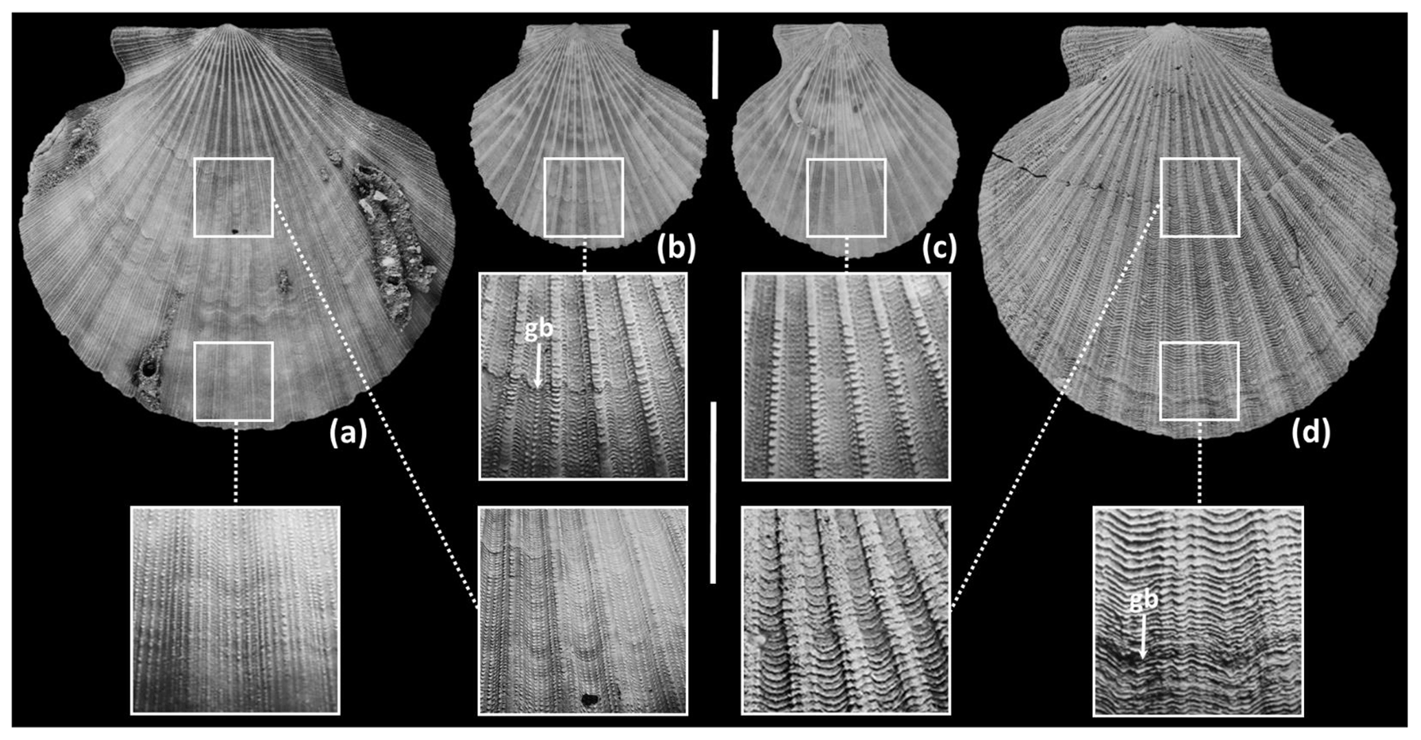
Figure 1 Pictorial demonstration of microgrowth-increment patterns in left valves of Aequipecten opercularis. (a) Typical supra-thermocline specimen (mesotidal setting, 23 m depth, La Coruña, Galicia, Spain) showing small increments early and late in ontogeny. (b, c) Typical sub-thermocline specimens (b microtidal setting, 50 m depth, Gulf of Tunis, Tunisia; c microtidal setting, 38 m depth, Adriatic Sea, Pula, Croatia) showing large increments early in ontogeny. (d) Inferred sub-thermocline specimen (Ramsholt Member, Coralline Crag Formation, Broom Pit, Suffolk, UK) showing large increments early in ontogeny and a transition from large to small increments late in ontogeny. Scale bars of 10 mm for whole-shell images (upper) and enlargements (lower). Major growth breaks (gb) identified in enlargements of (b, d). (a) University of Derby, Geological Collections (UD) 53424; (b) National Museum of Natural History, Paris, IM-2008-1542 (one of seven specimens in this lot); (c) UD 53423 (one of 48 specimens in this lot, coded S3A29); (d) UD 53425. See Johnson et al. (2009, 2021b) for numerical data and discussion of microgrowth-increment patterns in A. opercularis. Modern supra-thermocline specimens show a difference of <0.3 mm between the maximum and minimum values of smoothed increment-height profiles, while the majority of sub-thermocline specimens show a difference of >0.3 mm.

While δ¹⁸O sclerochronology is potentially informative about seasonality, it should be clear from the foregoing that results from the technique need to be interpreted carefully. The reliability of the information is of course also dependent on preservation of the original shell δ¹⁸O signature. Ivany and Judd (2022) provide a perspective on the issues considered above and in addition present a mathematical approach to reconstructing seasonality from the δ¹⁸O profiles of organisms whose growth rate is not uniform. This is, however, dependent on a strictly sinusoidal pattern of temperature variation over the year, which, as Ivany and Judd (2022) note, cannot be assumed in sub-thermocline situations (i.e. in the likely setting of some of the shells considered herein; see Sects. 3 and 5.3)

3 Setting and material

In the Pliocene the marine area of the SNSB was somewhat greater than now (Fig. 2), partly due to higher global sea level and partly to subsequent regional uplift (Westaway et al., 2002). Onshore marine deposits exist to the west in eastern England, and to the east in Belgium and the Netherlands, those in the last two countries passing eastwards into essentially fluvial non-marine deposits of the proto-Rhine–Meuse–Scheldt River system (Louwye et al., 2020; Munsterman et al., 2020). The Eridanos River system, draining the Baltic area, had its exit into the SNSB in the area of the present German Bight, some 400 km north-east of the proto-Rhine–Meuse–Scheldt exit (Gibbard and Lewin, 2016). While at certain times a link may have existed between the SNSB and the Channel Basin during the Pliocene (either at the present position or across southern England; Funnell, 1996; Westaway et al., 2002; van Vliet-Lanoë et al., 2002; Gibbard and Lewin, 2016), at others the basins were separated by the Weald–Artois land bridge, as shown in Fig. 2. Water depth in the southern North Sea is now less than 40 m in most places but seismic stratigraphy indicates that it was greater in the Pliocene, at least in areas of low sediment accumulation (Overeem et al., 2001).

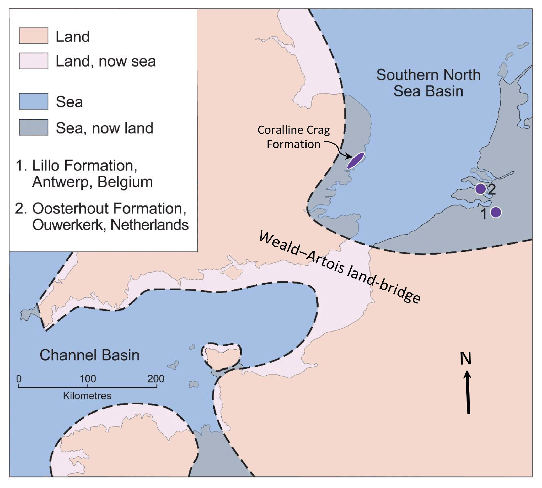
Figure 2 Pliocene palaeogeography in the vicinity of the SNSB, the location of sites in the Lillo (1) and Oosterhout (2) formations, from which shells were obtained, and the area of onshore outcrop of the Coralline Crag Formation in eastern England (the partly Pleistocene Red Crag Formation occurs over a larger area). Adapted from Valentine et al. (2011, Fig. 1), itself based on Murray (1992, map NG1).

In eastern England there is a large stratigraphic gap between the Zanclean Coralline Crag Formation and the late Piacenzian basal unit (“Walton Crag”) of the Red Crag Formation, but the Piacenzian is better recorded in northern Belgium by the Lillo Formation and in the south-west Netherlands by the Oosterhout Formation (Fig. 3). The last two formations essentially comprise marine sands, the Oosterhout Formation at Ouwerkerk (Zeeland) probably having been deposited in deeper water than the Lillo Formation at Antwerp from the evidence of fish otoliths (Gaemers and Schwarzhans, 1973) and a position farther from the inferred shoreline (Fig. 2). Nevertheless, Slupik et al. (2007) inferred a depth of deposition above storm wave base for most of the Oosterhout Formation at Schelphoek, 15 km north-west of Ouwerkerk. In the Antwerp area depth estimates based on the fauna have varied between authors according to the group studied, most of them hardly taking into account the marked variation in sediment and sedimentary structures within members of the Lillo Formation (see Deckers et al., 2020, Figs. 4–6). According to Gaemers (1975), the otolith assemblage indicates a depth of at least 10–20 m for the “Kallo Sands” (Lillo Formation, Oorderen Member; Marquet and Herman, 2009) but less than 10 m for the overlying Kruisschans Member. This indication of upward shallowing is supported by assemblage evidence from dinocysts (Louwye et al., 2004; De Schepper et al., 2009), Foraminifera (Laga, 1972), and bivalves (Marquet, 2004), but statistical data from the last group suggest greater absolute depths: 35–45 m for the Oorderen Member and 15–55 m for the Kruisschans Member by the common overlap in depth range of extant species; 40–50 m for the former and 20–50 m for the latter by the medial depth of extant species. The articulated preservation of the semi-infaunal bivalve Atrina fragilis, locally in life position, within the Oorderen Member (Marquet and Herman, 2009) is difficult to reconcile with the 10–20 m minimum depth estimate of Gaemers (1975), since specimens would have been subject to fair-weather processes after death. It is more likely that they lived at the depth suggested by Marquet (2004) and were killed by rapid burial (and permanently interred) in storms. A somewhat greater depth still was inferred from the bivalve assemblage of the underlying Luchtbal Member: 40–50 m by “common overlap”; 40–60 m by “medial depth”. The low diversity of the bivalve fauna of the Merksem Member (overlying the Kruisschans Member) precluded the same statistical treatment, but Marquet and Herman (2009) inferred from this impoverishment a depth of less than 15 m, an estimate consistent with the foraminiferal assemblage (Laga, 1972) and the high proportion of terrestrial palynomorphs (De Schepper et al., 2009).

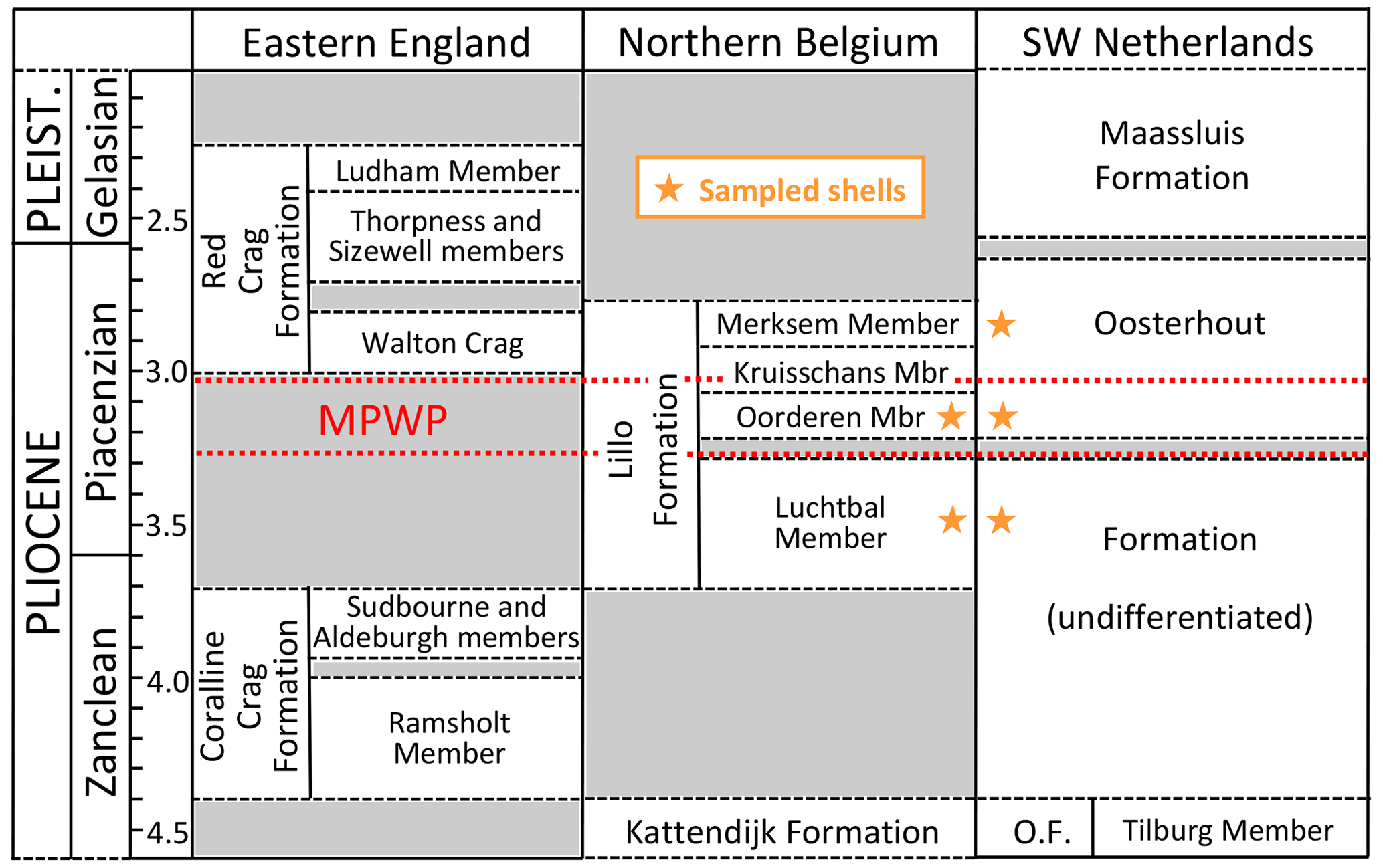
Figure 3 Stratigraphy and correlation of marine mid–late Pliocene and early Pleistocene units of the southern North Sea basin, with the general stratigraphic positions of shells sampled for the present study (specific positions in Table 1). Age (Ma) of the Red Crag Formation and constituent members (including the unofficial Walton Crag unit) according to Wood et al. (2009); of the Coralline Crag, Kattendijk and Lillo formations and constituent members according to De Schepper et al. (2009) and Louwye and De Schepper (2010); and of the Oosterhout (O.F.) and Maassluis formations according to Dearing Crampton-Flood et al. (2020) and Wesselingh et al. (2020). An additional small hiatus, of uncertain age, is present in the lower part of the Oosterhout Formation (Dearing Crampton-Flood et al., 2020). The Maassluis Formation includes a number of non-marine horizons (Slupik et al., 2007). Names of Lillo Formation members are in accordance with recent practice (Louwye et al., 2020; Wesselingh et al., 2020), omitting “Sand”/“Sands”, as included by previous authors. Wesselingh et al. (2020) found evidence of an additional layer (Broechem Unit) between the Kattendijk Formation and Luchtbal Member of the Lillo Formation. De Meuter and Laga (1976) designated an additional, uppermost division of the latter formation (Zandvliet Member), but this may be no more than the decalcified top of the Merksem Member (Louwye et al., 2020). Geographic provenance of shells and the location of the Coralline Crag Formation are shown in Fig. 2. MPWP: Mid-Piacenzian Warm Period.

Dinocyst assemblages indicate surface temperatures within the warm temperate range (but possibly only with respect to summer; Sect. 1) during the deposition of most of the Oorderen Member but punctuated by cool intervals and preceded by continuously cool conditions during the deposition of the Luchtbal Member (De Schepper et al., 2009). The dinocysts of the Kruisschans and Merksem members mainly indicate a continuation of the warm conditions of the Oorderen Member but provide a few hints of cooling (Louwye et al., 2004; De Schepper et al., 2009). Other evidence of this is provided by bivalves, fish, and pollen (Hacquaert, 1960; Vandenberghe et al., 2000; Marquet, 2005), and Wood et al. (1993) determined a 5–6 ^∘C decrease in summer surface temperature from the ostracods of a contemporaneous part of the Oosterhout Formation.

Previous sclerochronological investigation of late Pliocene temperatures in Belgium and the Netherlands focussed on the Oorderen Member and an equivalent horizon in the Oosterhout Formation and was restricted to δ¹⁸O data from two bivalve species: Aequipecten opercularis and Atrina fragilis (Valentine et al., 2011). Here we supplement the existing δ¹⁸O data from A. opercularis with microgrowth-increment data from the same specimens to gain an insight into their hydrographic setting (sub- or supra-thermocline), and we also supply δ¹⁸O data from two further bivalve species (Arctica islandica and Pygocardia rustica) from the Oorderen Member and another (Glycymeris radiolyrata) from the Luchtbal Member. In addition, we provide A. opercularis data from the Luchtbal Member and horizons equivalent to the Luchtbal and Merksem members in the Oosterhout Formation. Values for δ¹³C (obtained alongside δ¹⁸O) are reported for all species. Details of the provenance of the specimens are given in Table 1, together with alphanumeric codes (AO: A. opercularis; AI: A. islandica; PR: P. rustica; GR: G. radiolyrata) and sundry basic descriptive information. Note that the five specimens from the Oorderen Member sensu stricto come from the Atrina fragilis bed, a horizon with the warm temperate dinocyst assemblage found at most levels in the member. Illustrations of species other than A. opercularis (Fig. 1) are provided in Fig. 4. Most, if not all, of the material from the Lillo Formation was obtained from temporary exposures created during harbour works in the Antwerp area, while all the material from the Oosterhout Formation was obtained from a borehole (Rijkswaterstaat-Deltadienst, afdeling Waterhuishouding, 42H19-4/42H0039) at Ouwerkerk, Zeeland. Interpretation of positions (depths) within the Ouwerkerk borehole in terms of members within the Lillo Formation follows Gaemers and Schwarzhans (1973) except in the case of AO8, for which we have accepted the opinion of Frank Wesselingh (in Valentine et al., 2011) that the position is equivalent to the Oorderen Member. Gaemers and Schwarzans (1973) considered that strata of this age (Kallo Sands) were missing at Ouwerkerk, but they appear to be well represented at Schelphoek, only 15 km away (Slupik et al., 2007).

Table 1 Basic information for the investigated specimens (all single valves). Order stratigraphic within formations (by member, then by borehole depth or bed, with entries for the Oosterhout Formation inserted immediately above those, if any, for the equivalent member in the Lillo Formation). Entries in square brackets are interpretations (see footnotes). Latitudes and longitudes are for the location indicated in the adjacent column and do not necessarily specify the exact place of collection (see Fig. 2 for the positions of Ouwerkerk and Antwerp). UD: University of Derby, Geological Collections; IRSNB: Royal Belgian Institute of Natural Sciences, Brussels (MSNB was used for specimens discussed in Valentine et al., 2011).

^a No specific location indicated within Belgium but highly likely to be Antwerp. ^b Species indicated as “special” to the lower bed of the Luchtbal Member in the Deurganckdok (Marquet, 2002).

According to the latest chronostratigraphy (Fig. 3), the material investigated is largely or entirely Piacenzian (3.60–2.59 Ma) in age, the oldest (from the Luchtbal Member of the Lillo Formation) being possibly as old as 3.71 Ma (latest Zanclean) and the youngest (from horizons in the Oosterhout Formation equivalent to the Merksem Member of the Lillo Formation) being no younger than 2.76 Ma (De Schepper et al., 2009). The MPWP is probably represented by material from the Oorderen Member and the equivalent level in the Oosterhout Formation (Valentine et al., 2011). The Luchtbal and Oorderen members are separated by an unconformity interpreted by De Schepper et al. (2009) as a product of the sea-level fall associated with Marine Isotope Stage (MIS) M2 (ca. 3.3 Ma), which marks a glacial episode. The Luchtbal Member was therefore probably deposited before MIS M2 under interglacial conditions.

All the specimens come from stratigraphic intervals with a fully marine associated biota (e.g. Marquet, 2002, 2005; Gaemers and Schwarzhans, 1973), in conformity with modern occurrences in the case of the extant species A. opercularis and A. islandica (Tebble, 1976) and other fossil occurrences in the case of the extinct species P. rustica and G. radiolyrata (Norton, 1975; Buchardt and Simonarson, 2003; Marquet, 2002, 2005). Investigation of specimens of A. islandica, P. rustica, and G. radiolyrata added information from infaunal, slow-growing taxa to that derived from fast-growing, epifaunal A. opercularis, hence serving to mitigate any “ecological” bias in the results. We could not sample as many specimens of the infaunal, slow-growing species as of A. opercularis due to the limited availability of material (perforce from museums, in the lack of extant stratal exposures in the area of study). However, we sampled multiple years in the infaunal, slow-growing species, so the combined number of seasonal cycles investigated was similar to that in A. opercularis. We nevertheless expected some imbalance in the data because modern examples of Glycymeris species, from both cool- and warm-temperate settings, show winter cessation or slowing of growth and thus supply (or would supply) underestimates of the seasonal temperature range from δ¹⁸O sclerochronology (Peharda et al., 2012, 2019a, b; Royer et al., 2013; Reynolds et al., 2017; Featherstone et al., 2020; Alexandroff et al., 2021). Various equations have been used to express the precise relationship between δ¹⁸O and temperature in modern Glycymeris (Royer et al., 2013; Peharda et al., 2019a, b), but species of this genus certainly exhibit something at least close to equilibrium isotopic incorporation. The same is true of A. opercularis (Hickson et al., 1999; Johnson et al., 2021b) and A. islandica (Schöne, 2013; Mette et al., 2018; Trofimova et al., 2018). Because of the similarity of δ¹⁸O values from seemingly well-preserved P. rustica from the Pliocene of Iceland to those from co-occurring, similarly preserved A. islandica (Buchardt and Simonarson, 2003) it is reasonable to assume equilibrium fractionation in the former (extinct) species. The specimens analysed showed no physical signs of alteration, and they are unlikely to have been heated by more than 10 ^∘C through burial as the thickness of overlying sediments was probably never much more than 100 m (the depth below the present surface of the lowermost shell from the Ouwerkerk borehole). Examples of both calcitic A. opercularis (including AO7 herein) and aragonitic A. fragilis from the Lillo Formation were shown by Valentine et al. (2011) to exhibit the original shell microstructure. Similarly good preservation has been demonstrated in a variety of calcitic and aragonitic species from the slightly earlier Ramsholt Member of the Coralline Crag Formation in eastern England (Johnson et al., 2009; Vignols et al., 2019). We therefore considered it reasonable to proceed with isotopic analysis of our material (both calcitic and aragonitic; see Sect. 4 and Table 1) without detailed investigation of its preservation. Moon et al. (2021) have recently shown that good mineralogical and microstructural preservation does not necessarily guarantee good preservation of original shell δ¹⁸O. They heated shell material to 200 ^∘C and identified consistent negative shifts in δ¹⁸O (1.5 ‰ after 2 weeks at this temperature) over an annual cycle but no significant mineralogical or microstructural changes. As our specimens experienced only minimal heating through burial, similar alteration of shell δ¹⁸O is unlikely.

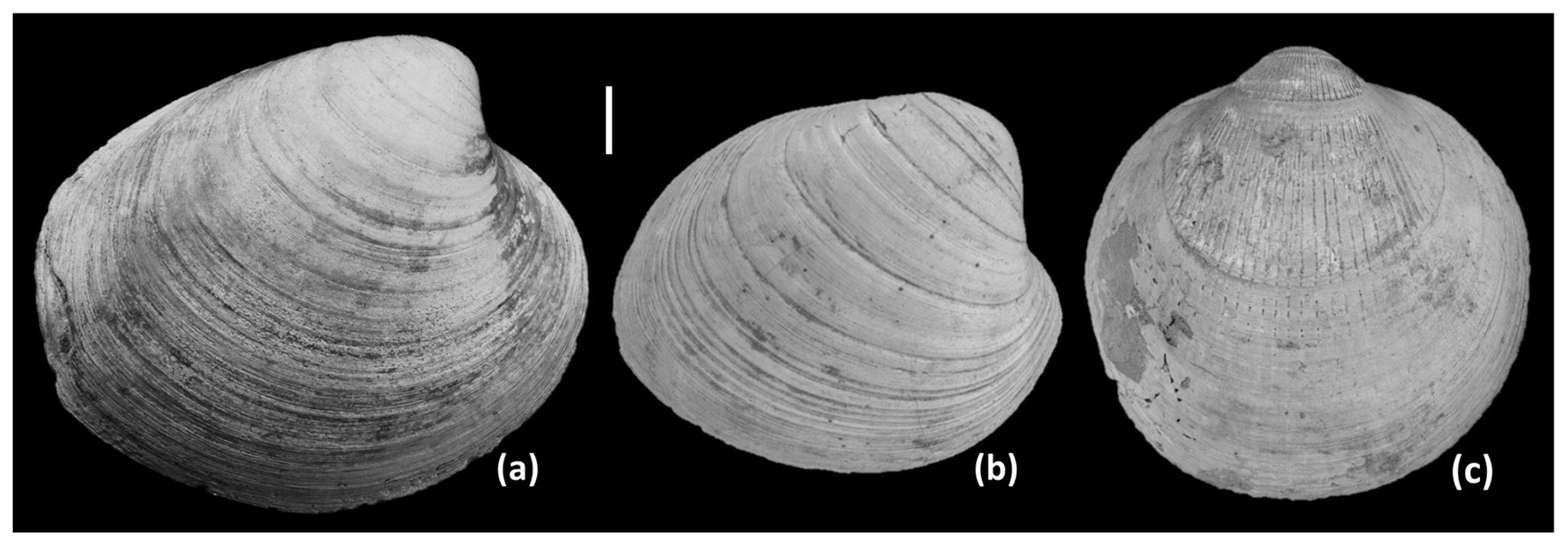
Figure 4 Right valves of (a) Arctica islandica, (b) Pygocardia rustica, and (c) Glycymeris radiolyrata from the Lillo Formation, Antwerp. (a) Probably Oorderen Member, Verrebroekdok (IRSNB 7699); (b) Oorderen Member, Verrebroekdok (IRSNB 7700); (c) Luchtbal Member, Deurganckdok (IRSNB 7701). Growth breaks are evident in all three specimens – e.g. ca. 10 major growth breaks in (b). Scale bar: 10 mm.

4 Methods

4.1 Laboratory procedures

The exterior of A. opercularis shells was coated with a sublimate of ammonium chloride and digitally photographed for the purpose of measuring microgrowth increments and the position of growth breaks. The coating was washed off with tap water and the shells then underwent the further cleaning procedure adopted by Valentine et al. (2011) for removal of any surficial organic matter, in preparation for isotopic sampling of the outer shell layer from the exterior, as in other such investigations of A. opercularis (e.g. Hickson et al., 1999, 2000; Johnson et al., 2009, 2021b; Vignols et al., 2019). The infaunal species were sampled in cross-section along the line of maximum growth, in accordance with universal practice for A. islandica (e.g. Schöne et al., 2005) and common practice for Glycymeris species (e.g. Royer et al., 2013). For this purpose shells were stabilized in resin before sectioning – by the partial-encasement method of Schöne et al. (2005) for A. islandica and P. rustica and the total-encasement method of Johnson et al. (2021a) for G. radiolyrata (fragments bonded beforehand). The use of vacuum impregnation in the latter method resulted in resin penetration into the outer part of the outer shell layer.

Extraction of isotope samples from A. opercularis shells was by drilling a dorsal to ventral series of shallow commarginal grooves (depth and width <1 mm; see Hickson et al., 1999, their Fig. 2; 2000, their Fig. 3) in the external surface, with the sample sites more closely spaced towards the ventral margin in an attempt to maintain temporal resolution in the face of declining growth rate with age. Details of the procedure are given in Johnson et al. (2019) with respect to another scallop species. Mean sample spacing for individuals – the average distance between the centres of grooves along the dorso-ventral (maximum-growth/shell-height) axis – was 0.93 (AO8)–1.35 (AO9) mm. Sampling of the infaunal species was by drilling a series of holes (depth and width <1 mm; Fig. 5) in the outer shell layer as seen in cross-section, the curved path being located about midway between the external surface and the boundary between the outer and inner shell layers in A. islandica and P. rustica but somewhat closer to the latter boundary in G. radiolyrata to avoid resin-contaminated material (Fig. 5). Sample spacing was more constant than for A. opercularis, although significantly reduced late in the long series from G. radiolyrata GR2, again to maintain temporal resolution. Mean sample spacing for individuals – the average distance between the centres of holes, measured in terms of the difference in straight-line distance from the origin of growth – was 0.69 mm for A. islandica, 0.57 mm for P. rustica, and 0.54 mm (GR2) and 0.57 mm (GR1) for G. radiolyrata. Note that in these relatively convex species the straight-line distance from the origin of growth is not a measurement of shell height as normally defined (a distance from the umbo, which protrudes dorsally of the origin of growth in these forms; e.g. Fig. 5) and that the plane in which it was measured (along the line of maximum growth) arguably does not include the shell-height axis in the prosogyrate species A. islandica and P. rustica (dependent on the point at the shell margin that is regarded as ventral). The lines of measurement and the values obtained are, however, regarded as “heights” for all four species considered herein, for the sake of simplicity. The A. opercularis shells were relatively small (Table 1) and were sampled from near the origin of growth (dorsal margin) to a point at or close to the ventral margin (maximum sample height 53.0 mm in AO10). The shells of the infaunal species were larger (Table 1) and not sampled to the end of ontogeny (maximum sample height 54.7 mm in GR2). Furthermore, the thinness of the outer layer close to the origin of growth meant that sampling had to start relatively far from this point (minimum sample height 15.4 mm in GR2).

Figure 5 Cross-section of Glycymeris radiolyrata specimen GR2 showing the origin of growth (og), position of sample holes (relatively far from the external surface in this species to avoid the darker, resin-contaminated material) and a major growth break (pale diagonal band in enlargement) at shell height 35.4 mm. Scale bars: 10 mm. Black spot in enlargement is a marker to assist sample numbering.

The cross-sections of the infaunal species were digitally photographed for the purpose of measuring the positions of sample holes and growth breaks, as seen on the shell exterior (Fig. 4) and projected or traced (Fig. 5) into the isotope sample path. Distances from the origin of growth were determined from the images using the bespoke measuring software Panopea (© 2004 Peinl and Schöne). Panopea was also used to measure the position of growth breaks and the height of microgrowth increments in the shell-exterior images of A. opercularis (see Fig. 1). As in the case of isotope sample positions, measurements were made along the dorso-ventral axis or (where this was impossible due to abrasion or encrustation) lateral to this line, the measurements then being mathematically adjusted as described by Johnson et al. (2019) to correspond to ones made along the dorso-ventral axis. All the microgrowth-increment measurements were made by the same person (Annemarie M. Valentine), thus assuring a reasonably uniform approach given the subjective element in increment identification (Johnson et al., 2021b). Growth breaks were classified as major (incorporating “moderate”) or minor in all species dependent on their external prominence (see Figs. 1, 4).

Samples (typically (50–100 µg) were analysed for their stable oxygen and carbon isotope composition (given as δ¹⁸O and δ¹³C) at the stable isotope facility, British Geological Survey, Keyworth, UK (A. opercularis, A. islandica, P. rustica), and the Institute of Geosciences, University of Mainz, Germany (G. radiolyrata). At Keyworth, samples were analysed using an Isoprime dual-inlet mass spectrometer coupled to a Multiprep system; powder samples were dissolved with concentrated phosphoric acid in borosilicate Wheaton vials at 90 ^∘C. At Mainz, samples were analysed using a Thermo Finnigan MAT 253 continuous-flow isotope ratio mass spectrometer coupled to a Gasbench II; powder samples were dissolved with water-free phosphoric acid in helium-flushed borosilicate exetainers at 72 ^∘C. Both laboratories calculated δ¹³C and δ¹⁸O against VPDB and calibrated data against NBS-19 (preferred values: +1.95 ‰ for δ¹³C, −2.20 ‰ for δ¹⁸O) and their own Carrara Marble standard (Keyworth: +2.00 ‰ for δ¹³C, −1.73 ‰ for δ¹⁸O; Mainz: +2.01 ‰ for δ¹³C, −1.91 ‰ for δ¹⁸O). Values were consistently within ±0.05 ‰ of the values for δ¹⁸O and δ¹³C in NBS-19. This confirms the comparability of results from each laboratory established in earlier work (Johnson et al., 2019). Note that δ¹⁸O of shell aragonite was not corrected for different acid-fractionation factors of aragonite and calcite (for further explanation, see Füllenbach et al., 2015).

4.2 Calculation of temperatures

In previous work on late Pliocene bivalves from Belgium and the Netherlands, minimum and maximum estimates of global average seawater δ¹⁸O (−0.5 ‰ and −0.2 ‰) and minimum and maximum modelled values for the early Pliocene in the western part of the SNSB (+0.1 ‰ and +0.5 ‰), all adjusted downwards by 0.1 ‰ to allow for the input of isotopically light freshwater into the eastern SNSB, were used to calculate sets of temperatures from shell δ¹⁸O (Valentine et al., 2011). It seems appropriate to apply the adjusted modelled values more widely to late Pliocene material from Belgium and the Netherlands. The adjusted global values are probably unreasonably low (they supply implausibly cold temperatures of 0.1 and 1.6 ^∘C, respectively, from AO6, a specimen from a horizon with a warm temperate dinocyst assemblage) and are not used here.

Valentine et al. (2011) employed the calcite equation of O'Neil et al. (1969) for the calculation of temperatures from A. opercularis, but there are grounds for thinking that this provides slightly inaccurate figures (Hickson et al., 1999; Vignols et al., 2019). The LL calcite equation of Bemis et al. (1998) seems to provide more accurate figures (i.e. for modern shells, a better fit with directly measured temperatures) and certainly yields a larger estimate for seasonal range (Johnson et al., 2021b). Both equations have therefore been employed herein to generate “minimum” and “maximum” seasonal ranges from A. opercularis. Note that the calcite equation of Kim and O'Neil (1997) yields an intermediate estimate, but the absolute temperatures obtained from modern A. opercularis are too low (Johnson et al., 2021b).

Just as there is some uncertainty as to the best equation for the calculation of temperatures from A. opercularis calcite, so different equations have been favoured for use with aragonitic Glycymeris glycymeris. Royer at al. (2013) advocated the use of a species-specific equation developed by them, while Reynolds et al. (2017) provide grounds for using the general aragonite equation of Grossman and Ku (1986). The former yields a smaller estimate of seasonal range than the latter so again both have been employed herein in relation to G. radiolyrata. The equation of Grossman and Ku (1986) is generally used in relation to aragonitic A. islandica and supplies similar temperatures from co-occurring (also aragonitic) P. rustica specimens (Buchardt and Simonarson, 2003). This, and no other equation, has therefore been used herein in relation to these species. In calculating temperatures appropriate adjustments were made to allow for the different scales used in measurement of water (VSMOW) and shell (VPDB) δ¹⁸O values (Coplen et al., 1983; Vignols et al., 2019).

5 Basic results and analysis

The isotopic, microgrowth-increment, and growth-break data are shown in Figs. 6 (Luchtbal Member and equivalent) and 7 (Oorderen Member and equivalent; Merksem Member equivalent). Read top to bottom, left to right (i.e. in the alphabetical order of parts), the sequence in each figure is as in Table 1, read top to bottom. The raw data are available online (Johnson et al., 2021c).

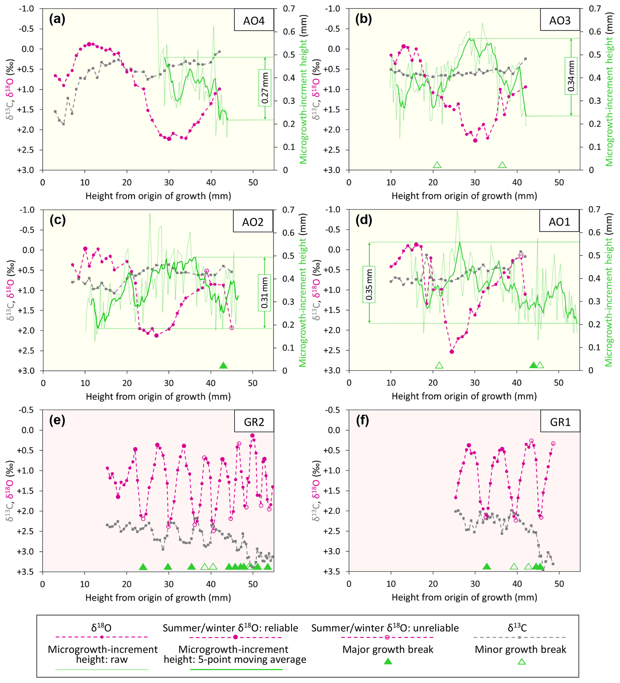
Figure 6 Ontogenetic profiles of δ¹⁸O, δ¹³C, and microgrowth-increment height from Luchtbal Member (and equivalent) A. opercularis (a–d) and G. radiolyrata (e, f). Note that the isotopic axis has been reversed in each part such that lower values of δ¹⁸O (corresponding to higher temperatures) plot towards the top. While the axis range is 4 ‰ throughout, the minimum and maximum values for A. opercularis (calcitic; pale yellow background) have been set 0.5 ‰ lower than for G. radiolyrata (aragonitic; pale pink background) to facilitate comparison, given the different fractionation factors applying for δ¹⁸O (Kim et al., 2007). The criteria for recognition of reliable and unreliable summer and winter δ¹⁸O values are given in Sect. 6.1.1. The fairly large single-point δ¹⁸O excursion at height 18.5 mm in (d) is matched by a negative one in δ¹³C and probably reflects contamination. Smaller interruptions of the large-scale cyclical pattern of δ¹⁸O variation in this and other profiles represent “noise” (unexplained variability).

5.1 δ¹⁸O values and growth breaks

Apart from departures representing probable contamination or “noise” (see Fig. 6d and caption), all profiles show cyclical patterns of δ¹⁸O variation, from less than half a cycle in A. opercularis profiles starting near the origin of growth and terminating at a height of about 30 mm (AO8, AO5 – Fig. 7c, f, respectively) to between two and three in a profile terminating at 53 mm (AO10 – Fig. 7a) but from between two and three cycles to substantially more over smaller height intervals in G. radiolyrata (between three and four from 25-49 mm in GR1 – Fig. 6f; between eight and nine from 15–55 mm in GR2 – Fig. 6e) and in P. rustica and A. islandica (between two and three from 27–48 mm in each case – Fig. 7g, h, respectively). In A. opercularis profiles extending beyond one δ¹⁸O cycle, the amplitude commonly shows a clear ontogenetic decrease. This pattern is less pervasive and pronounced amongst the other species, and the A. islandica specimen shows an ontogenetic increase in amplitude. However, the lack of early ontogenetic data for comparison from these species should be noted. The maximum amplitudes from G. radiolyrata specimens are less than from most A. opercularis specimens, but those from P. rustica and A. islandica are similar to A. opercularis. Growth breaks, albeit sometimes only minor, are associated with (<1 mm from the sample sites of) nearly all δ¹⁸O maxima and a few δ¹⁸O minima from G. radiolyrata but with none of the maxima or minima from A. opercularis. Growth breaks are associated with two of the three maxima and two of the three minima from the A. islandica specimen and with two of the three minima from the P. rustica specimen.

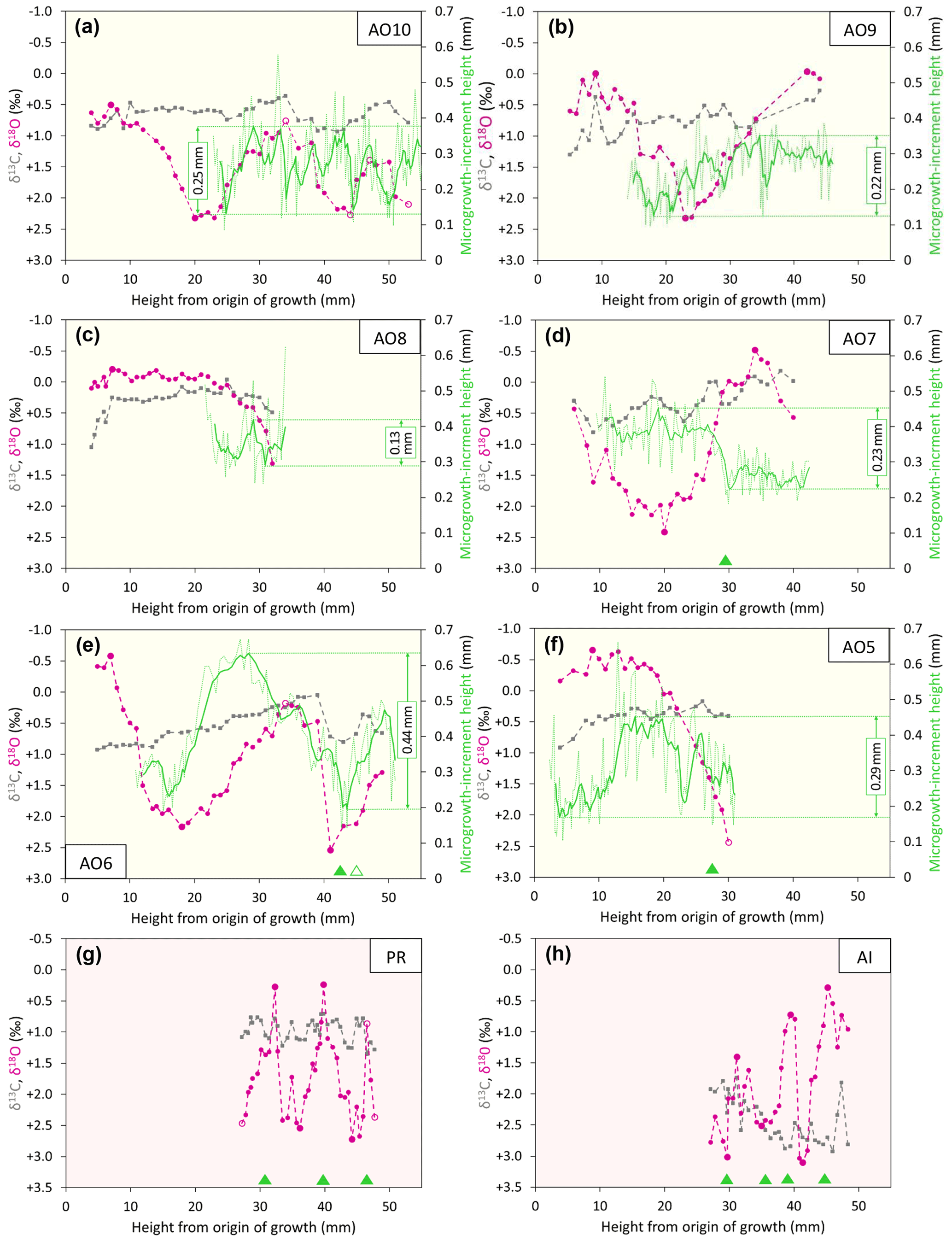
Figure 7 Isotopic, microgrowth-increment, and growth-break data from Merksem-equivalent A. opercularis (a, b) and Oorderen Member (and equivalent) A. opercularis (c–f), P. rustica (g), and A. islandica (h). Format and symbols as in Fig. 6.

Taking the δ¹⁸O cycles to reflect seasonal temperature variation and hence intervals of 1 year, the much smaller number over a given height interval from A. opercularis confirms that this species grew a great deal faster than the others (more than twice as fast as A. islandica and P. rustica and 3 to 5 times faster than G. radiolyrata). In A. opercularis profiles spanning 2 or more years (AO10, AO6 – Fig. 7a, e, respectively), there is an ontogenetic decrease in wavelength as well as amplitude – i.e. growth was fastest in early ontogeny. Ontogenetic decline in growth rate has been widely documented in A. opercularis from both δ¹⁸O and other evidence (e.g. Johnson et al., 2021b), and in the present instances (in which δ¹⁸O maxima and minima are not associated with growth breaks) the ontogenetic decrease in amplitude of δ¹⁸O cycles is probably a consequence of the general slowing of growth with age, leading to time averaging in samples. Whatever the explanation, seasonal temperature variation is likely to be most faithfully reflected by the first δ¹⁸O cycle in A. opercularis profiles. The profiles from G. radiolyrata, P. rustica, and A. islandica undoubtedly omit several early ontogenetic cycles and given the short wavelength of the later cycles represented, it may be that the amplitude of these is reduced by time averaging, as inferred in A. opercularis. Even if the closer spacing of samples from G. radiolyrata, P. rustica, and A. islandica may have been sufficient in principle for the resolution of seasonal δ¹⁸O extremes, the association of growth breaks with maxima, minima, or both suggests that some recorded extremes are not representative of the most extreme temperatures experienced by the organism in the season concerned – i.e. δ¹⁸O variation may not fully reflect seasonal temperature variation.

5.2 δ¹³C values

Compared to δ¹⁸O values from the same specimen, δ¹³C values generally show much less variation, particularly within the span of δ¹⁸O cycles. Nevertheless, in some specimens there are intervals exhibiting covariation between δ¹³C and δ¹⁸O: moderate–strong positive covariation in AO10 (Fig. 7a), AO6 (Fig. 7e), and PR (Fig. 7g) between shell heights 25 and 53 mm (r²=0.61), 18 and 46 mm (r²=0.84), and 31 and 46 mm (r²=0.34), respectively; moderate–strong negative covariation in GR2 (Fig. 6e) and GR1 (Fig. 6f) between shell heights 25 and 43 mm (r²=0.68) and 26 and 42 mm (r²=0.40), respectively. However, the general picture is of fluctuations (if any) in δ¹³C that are independent of δ¹⁸O. The A. opercularis specimens show a marginal to clear overall decrease in δ¹³C through ontogeny, while the P. rustica specimen shows little change and the A. islandica and G. radiolyrata specimens show clear overall increases. The mean values from the A. opercularis specimens are very similar – from $+\mathrm{0.31}\pm \mathrm{0.22}$ ‰ (±1σ) in AO8 to $+\mathrm{0.77}\pm \mathrm{0.24}$ ‰ in AO9 – and comparable to the mean from the P. rustica specimen ($+\mathrm{0.98}\pm \mathrm{0.18}$ ‰) but much lower than the means from the A. islandica ($+\mathrm{2.44}\pm \mathrm{0.35}$ ‰) and G. radiolyrata (GR1, $+\mathrm{2.42}\pm \mathrm{0.40}$ ‰; GR2, $+\mathrm{2.69}\pm \mathrm{0.32}$ ‰) specimens. The data from A. opercularis and A. islandica compare closely with those from early Pliocene examples of these species from eastern England (Johnson et al., 2009; Vignols et al., 2019). The difference between the means from early Pliocene A. opercularis (calcitic) and A. islandica (aragonitic) was ascribed principally to the mineralogical difference (Vignols et al., 2019). This interpretation is supported by the mean values from the present G. radiolyrata (aragonitic) specimens, which are similar to those from A. islandica, but not by the P. rustica (also aragonitic) mean value, which is only a little outside the range of mean values from A. opercularis. The different pattern of overall ontogenetic change in G. radiolyrata and A. islandica (increase, unlike in A. opercularis and P. rustica) also remains to be explained, as does the unusual negative covariation between δ¹³C and δ¹⁸O in G. radiolyrata.

5.3 Microgrowth-increment patterns (A. opercularis)

Even in smoothed (five-point moving average) profiles of microgrowth-increment size from A. opercularis, substantial high-frequency variation is present in nearly all cases. However, amongst those profiles long enough to show a low-frequency pattern, in a number of cases a fairly clear and complete major cycle proceeding from small to large to small increments is discernible over about the first 40 mm of shell height. Such a cycle is evident in three of the four Luchtbal Member (and equivalent) profiles, in each case with an amplitude (difference between the maximum and minimum of the smoothed profile) of more than 0.30 mm. The exception (AO4 – Fig. 5a) is a profile too short to show this pattern. Only one (AO6 – Fig. 6g) of the four Oorderen Member (and equivalent) profiles has an amplitude greater than 0.30 mm, but a second (AO5 – Fig. 6f) has an amplitude only fractionally less and a third (AO8 – Fig. 6c) is too short to show equivalent (“high-amplitude”) variation. Despite their considerable length the Merksem-equivalent profiles exhibit an amplitude well below 0.30 mm (“low amplitude”). The prevalent high-amplitude pattern from Luchtbal Member (and equivalent) shells corresponds to that in modern sub-thermocline shells, and the occurrence of the pattern in an Oorderen Member shell is at least inconsistent with a supra-thermocline setting (Johnson et al., 2009, 2021b). The low-amplitude pattern in the two Merksem-equivalent shells is consistent with a supra-thermocline setting; however, given the occasional occurrence of such a pattern in sub-thermocline shells, it is not inconsistent with the latter setting.

6 Interpretation

6.1 Temperatures

6.1.1 Derivation, comparison, and evaluation of seasonal seafloor values

The equations and water δ¹⁸O values that were employed to calculate summer and winter temperatures from shell δ¹⁸O are explained in Sect. 4.2. Following the reasoning of Johnson et al. (2017), the shell δ¹⁸O values used were the extreme ones at inflection points in profiles, supplemented in the present case by those profile-end values possibly corresponding to inflection points on the evidence of similar (true) inflection-point values from the same and other co-occurring shells of the species concerned. The profile-end values probably provide slight underestimates of summer temperature and slight overestimates of winter temperature in some cases – i.e. had the profiles extended farther, slightly lower or higher δ¹⁸O values, respectively, might have been identified. As well as errors from this source, others of the same type no doubt exist in the case of data from locations close to growth breaks (as a result of an incomplete record) and, for at least A. opercularis, in the case of late ontogenetic data (as a result of time averaging), although no significant error is likely where the temperatures concerned are higher (for summers) or lower (for winters) than a reliable estimate from another time in ontogeny. Alongside the profile-end and near-growth-break (unreliable) winter δ¹⁸O data from G. radiolyrata is one inflection-point value (the first, unaccompanied by a growth break, at a height of 17.9 mm in GR2; Fig. 6e) which appears acceptable as a source of reliable temperature information. The δ¹⁸O value is, however, lower than any from this taxon regarded as an unreliable source of winter temperatures. Hence, it too must be regarded as suspect, possibly recording a downward temperature fluctuation in spring rather than true winter conditions.

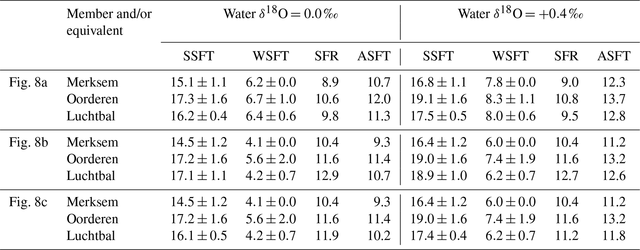
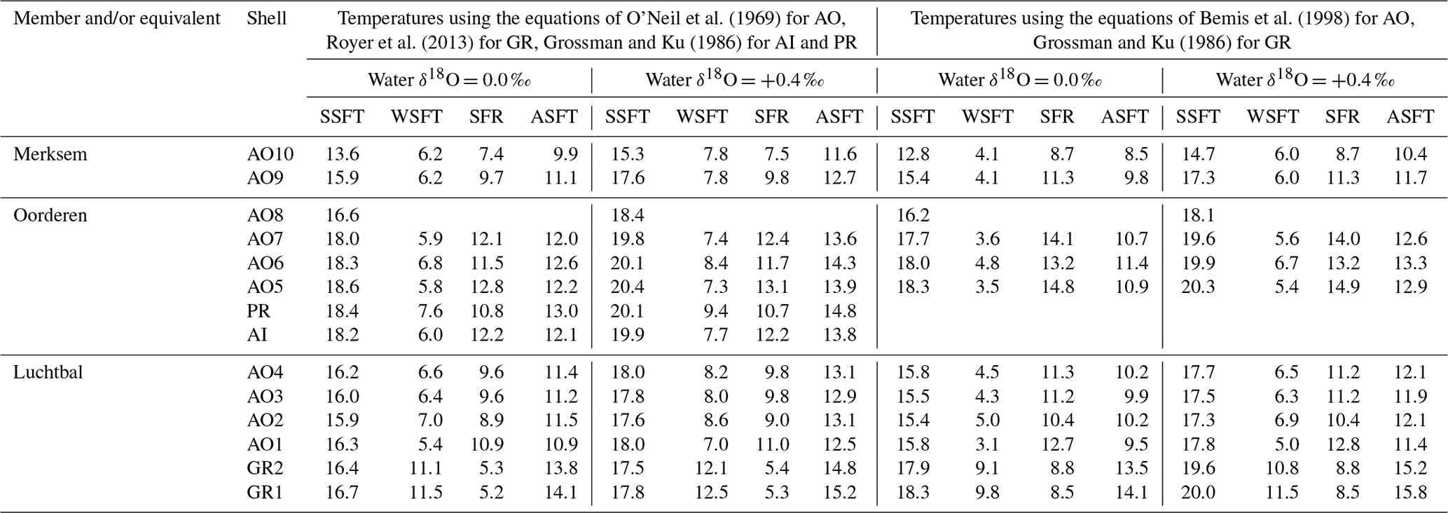
All the calculated temperatures are represented in Fig. 8, those based on equations providing minimum seasonal ranges for G. radiolyrata and A. opercularis combined in Fig. 8a, those providing maximum seasonal ranges for these species combined in Fig. 8b, and those providing a minimum seasonal range for G. radiolyrata and a maximum for A. opercularis (a “hybrid” set) combined in Fig. 8c. Unreliable values (probable underestimates for summers and overestimates for winters) are identified by the use of an open symbol, whereby we have applied the above reasoning uniformly except to G. radiolyrata, A. islandica, and P. rustica: in the absence of early ontogenetic data for comparison in these species, we have assumed that the late ontogenetic data represented are free from time-averaging effects.

Figure 8 Winter and summer seafloor temperatures, calculated from the seasonal extreme δ¹⁸O values indicated in Figs. 6 and 7, using water δ¹⁸O values of 0.0 ‰ and +0.4 ‰ and various equations. (a) Equation of Royer et al. (2013) for GR, of O'Neil et al. (1969) for AO and of Grossman and Ku (1986) for AI and PR; (b) equation of Grossman and Ku (1986) for GR, AI, and PR and of Bemis et al. (1998) for AO; (c) equation of Royer et al. (2013) for GR, of Bemis et al. (1998) for AO, and of Grossman and Ku (1986) for AI and PR. Interval means are for reliable seasonal temperatures (see Sect. 6.1.1) from the Luchtbal Member and equivalent, Oorderen Member and equivalent, and Merksem-equivalent strata. The indicated present-day seasonal seafloor temperature range (4.7–16.9 ^∘C) is for 25 m depth at 53^∘ N, 03^∘ E.

Figure 8 shows a general similarity in seasonal temperatures within and between stratigraphic members, with the exception of winter values supplied by G. radiolyrata from the Luchtbal Member, which are markedly higher than those from Luchtbal Member A. opercularis. Since the specimens of each species come from different (although immediately adjacent) beds, it is conceivable that the data reflect environmental change. However, given the fact that the summer temperatures supplied by the species are close or identical (dependent on the method of calculation) and that all of the 12 sets of winter temperatures from G. radiolyrata are probable overestimates, it seems much more likely that the change is apparent rather than real. If this is accepted then it is sensible to view those Luchtbal Member (and equivalent) summer temperatures represented in Fig. 8a and c (very similar from G. radiolyrata and A. opercularis for the same water δ¹⁸O value) as more accurate than those in Fig. 8b (somewhat lower from A. opercularis than from G. radiolyrata for the same water δ¹⁸O value). The Oorderen Member winter temperatures from A. islandica and P. rustica are closer to those from Oorderen Member A. opercularis (from the same bed) in Fig. 8a than those in Fig. 8c (and Fig. 8b), suggesting that the data in Fig. 8a are the most accurate overall. However, if it is untrue that the winter data from A. islandica and P. rustica are free from time-averaging effects (i.e. if the data are unreliable), there is no reason for favouring the remaining data in Fig. 8a over those in Fig. 8c.

Table 2 gives the interval mean values for seasonal temperatures based on reliable data, as depicted in Fig. 8. Unlike other changes, the Luchtbal to Oorderen increases and the Oorderen to Merksem decreases in mean summer temperature evident in Fig. 8a and c are statistically significant for both water δ¹⁸O values (one-tailed t tests; p<0.05). The fact that these changes correspond at least qualitatively to the changes in summer temperature inferred from dinocysts and ostracods (Sect. 3) cements the impression that the data in Fig. 8a and c provide a more accurate picture of seasonal temperatures, and hence of seasonal range, than the data in Fig. 8b, in which only the Oorderen to Merksem decrease in summer temperature (again statistically significant) is evident.

Table 2 Mean summer (SSFT) and winter (WSFT) seafloor temperatures (^∘C; ±1σ), seasonal range (SFR: SSFT minus WSFT), and annual average temperature (ASFT: midpoint between SSFT and WSFT) for “members”, based on the reliable data indicated in Fig. 8.

In conclusion, the data in Fig. 8a are probably the most accurate, but the data in Fig. 8c should not be excluded from consideration, especially as evidence from modern A. opercularis (Johnson et al., 2021b) suggests that the equation of Bemis et al. (1998), used for the calculation of temperatures from this species in Fig. 8c, provides more accurate temperatures than the equation of O'Neil et al. (1969), used in Fig. 8a.

6.1.2 Seasonal seafloor ranges

With the exception of the Luchtbal values resulting from the questionable combination of data employed in Fig. 8b, all the seasonal ranges for members (irrespective of how data have been combined and temperatures calculated; Table 2) are lower than the current seafloor range at offshore locations in the southern North Sea – e.g. at 53^∘ N, 03^∘ E, where the difference between mean maximum and minimum temperatures is 12.2 ^∘C (Johnson et al., 2021b, their Fig. 1a). However, they are only slightly lower (compare the separations of the dotted/dashed lines in Fig. 8 with the width of the grey bar showing the current range at 53^∘ N, 03^∘ E), and not all individual specimens indicate a lower range (Table 3): the A. islandica specimen (Oorderen Member) shows the same range as currently at 53^∘ N, 03^∘ E, and even a water δ¹⁸O value of 0.0 ‰ used with the equation of O'Neil et al. (1969) yields a range (12.8 ^∘C) from the Oorderen A. opercularis specimen AO5 that is higher than at present. The latter case is based on a winter temperature that is not reliable in the sense of Sect. 6.1.1, but the true (most extreme) winter temperature can only have been less and the seasonal range hence greater. Using a water δ¹⁸O value of +0.4 ‰ with the equation of O'Neil et al. (1969) yields a range of 12.4 ^∘C from the Oorderen specimen AO7, and using the equation of Bemis et al. (1998) yields a range of 13.2 ^∘C from the Oorderen specimen AO6 and 12.8 ^∘C from the Luchtbal specimen AO1 (independent of water δ¹⁸O) as well as higher ranges than with the equation of O'Neil et al. (1969) from the Oorderen specimens AO5 (14.9 ^∘C) and AO7 (14.0 ^∘C). It can therefore be said that at times during the period of deposition of the Oorderen Member, and possibly of the Luchtbal Member, the seasonal range in seafloor temperature was higher than the current typical range. One should, however, bear in mind the variation of about 2 ^∘C either side of the mean maximum and minimum temperatures in the North Sea at present (Lane and Prandle, 1996), so the “high” individual Oorderen and Luchtbal ranges do not necessarily manifest significantly greater seasonality than now. Individual specimens from the equivalent of the Merksem Member provide some evidence of a lower seafloor range than now (maximum range 11.3 ^∘C from AO9, calculated with the equation of Bemis et al., 1998), but the small sample size (two) should be noted.

Table 3 Summer (SSFT) and winter (WSFT) seafloor temperatures (^∘C) for the year showing the greatest range (SFR; SSFT minus WSFT) from each shell, together with the annual average seafloor temperature (ASFT; midpoint between SSFT and WSFT). Unreliable as well as reliable seasonal temperatures used (Fig. 8). AO8 (no winter data) has been included to supplement the summer data.

The calculations leading to the above figures for seasonal range assume constant water δ¹⁸O during the intervals of ontogeny concerned. If at the times of maximum temperature the actual water δ¹⁸O value was lower than assumed the calculated temperatures would be overestimates; similarly, if at the times of minimum temperature the actual water δ¹⁸O value was higher than assumed the calculated temperatures would be underestimates. Each of these situations, or the two together, would yield an overestimate of seasonal range. While these circumstances are possible, they are improbable. As noted in Sect. 2, water δ¹⁸O is relatively high (not low) during summer and relatively low (not high) during winter in coastal waters of the North Sea at present. The calculated seasonal ranges are thus more likely to be underestimates.

6.1.3 Seasonal surface ranges

The water depths indicated by the bivalve mollusc assemblages of the Luchtbal and Oorderen members (respective minimum depths 40 and 35 m; Sect. 3) are greater than the typical depth of the summer thermocline in shelf settings (25–30 m). Microgrowth-increment evidence from A. opercularis (Sect. 5.3) is consistent with a sub-thermocline setting for both members, and the higher frequency of such evidence from the Luchtbal Member is consistent with the indication from assemblage analysis that this was deposited at a greater depth than the Oorderen Member. Microgrowth-increment evidence of a supra-thermocline setting from Merksem-equivalent shells in the Oosterhout Formation at Ouwerkerk is similarly consistent with the shallow depth of deposition (maximum 15 m) indicated by the biota of the Merksem Member itself at Antwerp (note that supra-thermocline settings exist now in the southern North Sea at a distance from the shore well beyond that of Ouwerkerk from the Pliocene shoreline; Fig. 2). Given a sub-thermocline setting for the Luchtbal and Oorderen members we must add a “stratification factor” to summer seafloor temperatures to derive estimates of summer surface temperature and hence seasonal surface range (winter surface temperature is likely to have been the same as on the seafloor; Johnson et al., 2021b). There is a difference of 2.6 ^∘C between the mean annual seafloor and surface temperature maxima at a seasonally stratified location (depth 59 m) in the central North Sea some 600 km north of the sites of the Pliocene shells (Johnson et al., 2021b). At this location the mean maximum surface temperature is only 13.7 ^∘C, a figure substantially exceeded in the (unstratified) southern North Sea at present (e.g. 17.1 ^∘C at 53^∘ N, 03^∘ E; Johnson et al., 2021b, their Fig. 1a) and with little doubt at warm times during the deposition of the Oorderen Member (see Sect. 3). From the evidence of dinocysts (De Schepper et al., 2009) it is conceivable that at cool times, and during the deposition of the Luchtbal Member, summer surface temperature was not much higher than the present central North Sea figure. A stratification factor of 3 ^∘C is therefore a reasonable estimate for these cool intervals and a serviceable (conservative) one for warm intervals during the deposition of the Oorderen Member. Adding 3 ^∘C to the interval mean values for Luchtbal and Oorderen summer seafloor temperature yields stratification-adjusted figures for seasonal surface range (Table 4) that are in all cases higher than the present typical range in the southern North Sea (12.4 ^∘C at 53^∘ N, 03^∘ E; Johnson et al., 2021b). Adding the same to individual values also yields figures for seasonal surface range (Table 5) that are higher than the present typical range, except in the cases of Luchtbal specimens GR1, GR2, and AO2. A lower range is only obtained from the last when benthic temperature is calculated using the equation of O'Neil et al. (1969), and the lower ranges from GR1 and GR2 reflect the high winter seafloor temperatures recorded, all of which are unreliable. While the Luchtbal and Oorderen (and respective equivalent) shells provide clear evidence of a higher surface range than now (see Fig. 9, which depicts the interval mean and individual information from Tables 4 and 5), a lower range is indicated by the two Merksem-equivalent shells, assuming these have been correctly interpreted as from a supra-thermocline setting. It may of course be the case that they provide an unrepresentative picture for their time.

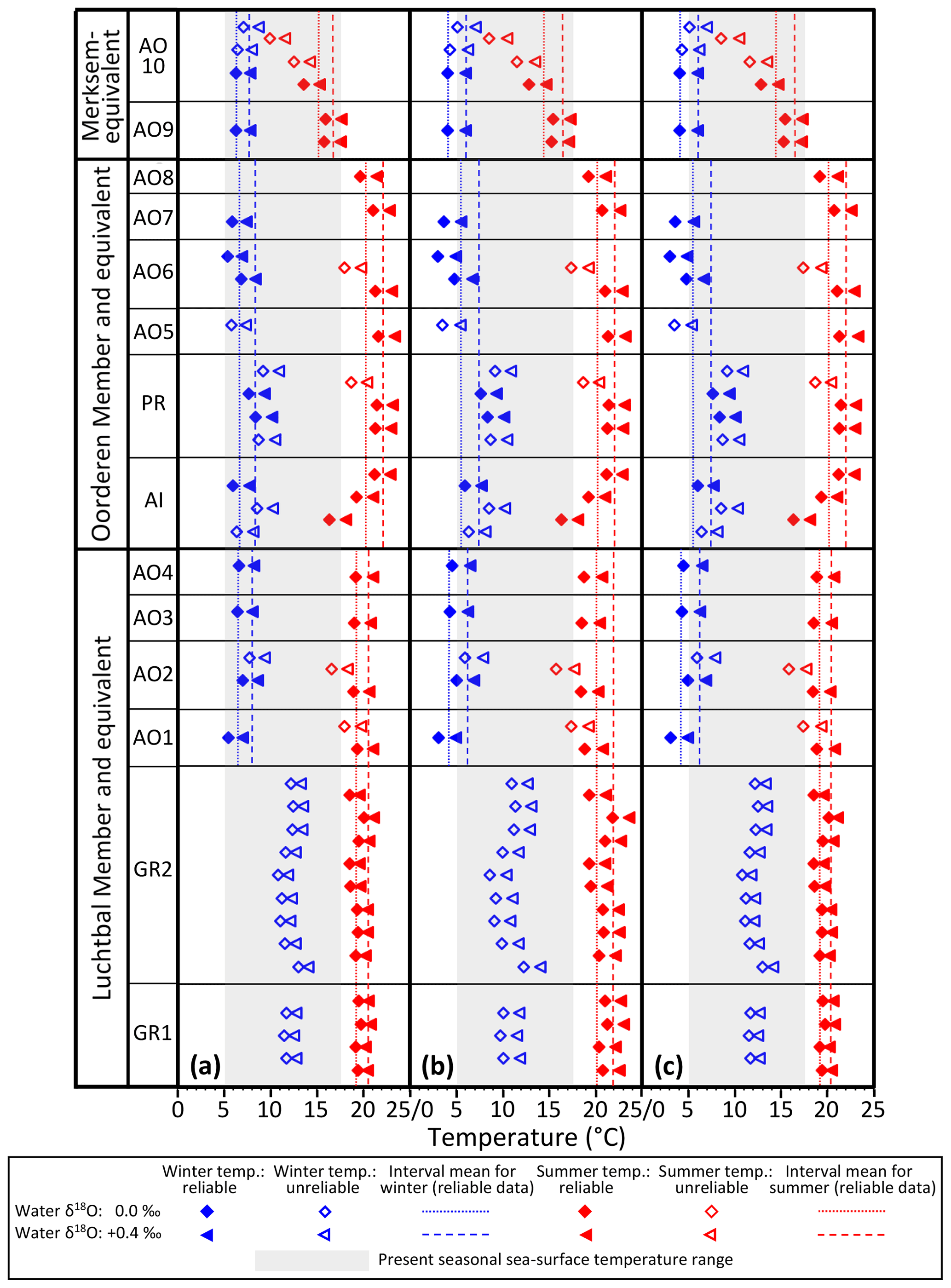
Figure 9 Winter and summer sea surface temperatures, calculated as in Fig. 8, using the same equations for (a), (b), and (c) but with a 3 ^∘C supplement to Luchtbal and Oorderen summer temperatures in recognition of thermal stratification (see text, Sect. 6.1.3, for explanation). Interval means calculated as in Fig. 8. The indicated present-day seasonal sea surface temperature range (4.7–17.1 ^∘C) is for 53^∘ N, 03^∘ E. Note that the Luchtbal and Oorderen ranges, as indicated by the separation of dotted or dashed lines for each interval, are larger than the present-day range (see text, Sect. 6.1.3, for more detailed discussion).

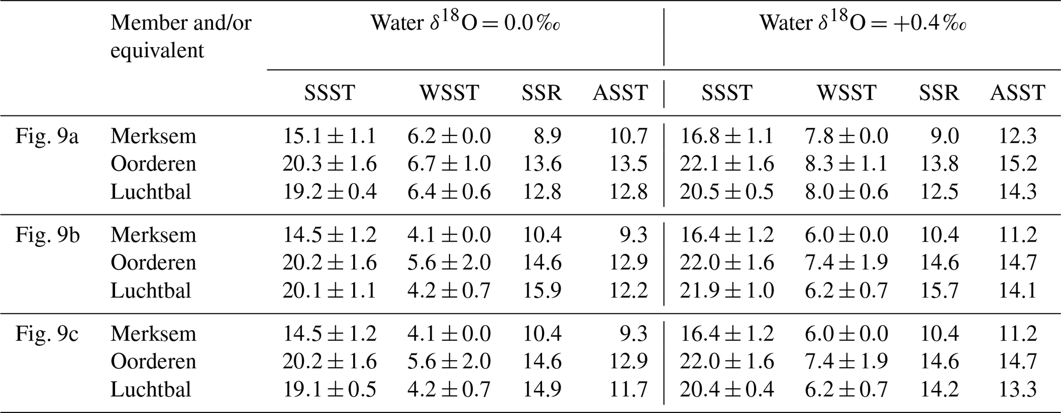
Table 4 Mean summer (SSST) and winter (WSST) sea surface temperatures (^∘C; ±1σ), seasonal range (SSR: SSST minus WSST), and annual average temperature (ASST: midpoint between SSST and WSST) for “members”, based on the reliable data indicated in Fig. 8, with a 3 ^∘C addition to Luchtbal and Oorderen summer seafloor temperatures in recognition of summer stratification (see text, Sect. 6.1.3, for explanation).

6.1.4 Absolute surface temperatures

As pointed out in Sect. 6.1.1, there is a Luchtbal–Oorderen increase and an Oorderen–Merksem decrease in mean summer seafloor temperature from reliable individual summer values calculated using the equation of Royer et al. (2013) for G. radiolyrata, the equation of Grossman and Ku (1986) for A. islandica and P. rustica, and the equations of both O'Neil et al. (1969) and Bemis et al. (1998) for A. opercularis. These changes are evident whether a water δ¹⁸O value of 0.0 ‰ or +0.4 ‰ is applied, are statistically significant, and correspond qualitatively to changes in summer temperature inferred from assemblages of ostracods and dinocysts. These proxies (and organic biomarkers – see below) provide estimates that are time-averaged to much the same extent as the interval-mean seasonal temperatures quoted herein, making comparison fair. The data from ostracods and probably from dinocysts relate to summer sea surface temperature (SSST), so quantitative comparison must involve the equivalent data, derived as indicated in Sect. 6.1.3. The relevant interval mean information is that for Fig. 9a and c in Table 4, showing Oorderen SSST above 20 ^∘C and Merksem SSST below 20 ^∘C, irrespective of the water δ¹⁸O value used in calculation, and Luchtbal SSST above 20 ^∘C with a water δ¹⁸O value of +0.4 ‰ and below 20 ^∘C with a water δ¹⁸O value of 0.0 ‰. All the Oorderen SSST estimates are consistent with dinocyst evidence (Sect. 3) specifying mainly warm temperate conditions (SSST >20 ^∘C; Johnson et al., 2021b), and the Luchtbal SSST estimates with a water value of 0.0 ‰ are consistent with dinocyst evidence specifying cool temperate conditions (SSST <20 ^∘C; Johnson et al., 2021b). This suggests that temperatures calculated with a water δ¹⁸O value of 0.0 ‰ may be the most accurate for all intervals. The Merksem interval mean SSST calculated with this value is 14.5 or 15.1 ^∘C dependent on the equation used (Table 4), both figures being consistent with the Oorderen–Merksem SSST decrease of 5–6 ^∘C indicated by ostracod assemblage data (Sect. 3). The statements made in respect of interval means also apply in general to individual SSST values calculated with the same equations (Table 5). The only exceptions are the temperatures derived using a water δ¹⁸O value of 0.0 ‰ from Oorderen specimen AO8, which are slightly below the warm temperate range for summer. Such temperatures are entirely to be expected from some individuals in a regime with a mean SSST only a few degrees above the cool temperate range (see Sect. 6.1.2).

The similarity of δ¹⁸O-derived estimates of summer sea surface temperature, particularly those using a water δ¹⁸O value of 0.0 ‰, to assemblage-based estimates lends credence to the equivalent winter sea surface temperatures (WSSTs). With the exception only of unreliable individual data from G. radiolyrata, all WSST estimates (Tables 4, 5) are firmly in the cool temperate range (<10 ^∘C; Johnson et al., 2021b). We can take the midpoint between interval mean SSST and WSST estimates as a figure for annual (“average”) sea surface temperature (ASST) and compare this with ASST estimates based on other information. Robinson et al. (2018) derived an ASST of 13.6 ^∘C for the mid-Piacenzian North Sea using bivalve δ¹⁸O data from the Coralline Crag Formation (UK). It is, however, questionable whether the Coralline Crag is of this age (see Fig. 3). Dearing Crampton-Flood et al. (2020) obtained an SSST of about 16 ^∘C (cool temperate) from alkenone index and a WSST of about 10 ^∘C (boundary cool–warm temperate) from TEX₈₆ for part of the Oosterhout Formation in the Netherlands (Noord-Brabant) representing the MPWP. These figures specify an ASST of 13 ^∘C. This is very similar to the δ¹⁸O-derived ASST estimates (Table 4) of 12.9 and 13.5 ^∘C obtained using a water δ¹⁸O value of 0.0 ‰ from Oorderen and equivalent shells, which represent the same interval. Such figures for ASST (2–3 ^∘C higher than the modern ASST of 10.9 ^∘C specified by an SSST of 17.1 ^∘C and WSST of 4.7 ^∘C at 53^∘ N, 03^∘ E; Johnson et al., 2021b, their Fig. 1a) are entirely consistent with general expectations for the MPWP, but the δ¹⁸O-derived data reveal that they result from substantially warmer summer conditions than at present and winter conditions much the same as now, opposite to the picture provided by alkenone and TEX₈₆ data. The interval mean Luchtbal figures for SSST obtained using a water δ¹⁸O value of 0.0 ‰ are likewise above the present SSST, although less markedly so, and in combination with WSST figures similar to the present also specify a higher ASST than now (Table 4). By contrast, the equivalent Merksem figures for SSST are below the present value and in combination with WSST figures similar to the present specify a lower ASST than now.

6.2 Meaning of δ¹³C data

The ontogenetic decline in δ¹³C shown by A. opercularis is as seen in modern examples of the species from diverse settings (Johnson et al., 2021b) and probably reflects increasing output of isotopically light respiratory carbon with increasing body size alongside slower shell secretion – i.e. reduced “demand” for carbon (Lorrain et al., 2004). Short-term fluctuations paralleling changes in δ¹⁸O might similarly reflect variation in respiratory output determined by seasonal variation in the availability of food (Chauvaud et al., 2011). The opposite ontogenetic trend shown by G. radiolyrata and A. islandica can hardly be explained by a reduction in respiratory output, and the opposite short-term pattern shown by G. radiolyrata is unlikely to reflect a reversal in the timing of maximum food availability from summer to winter. These changes might reflect variation in the δ¹³C of dissolved inorganic carbon (DIC), the main source of carbon in shells (Marchais et al., 2015). Preferential uptake of ¹²C by photosynthesizers is a major influence on the δ¹³C of DIC, but high photosynthetic fixation of carbon in summer is a doubtful cause of the high summer δ¹³C values in G. radiolyrata because it would require (see Arthur et al., 1983) that the shells lived above the thermocline, which other evidence argues against. The anomalously low δ¹³C values from P. rustica (for the aragonite mineralogy) cannot be explained as a consequence of the incorporation of isotopically light carbon from porewaters (cf. Krantz et al., 1987) because the other infaunal species, G. radiolyrata and A. islandica, exhibit high values. Conceivably, the P. rustica values reflect a food source with a particularly low value (Marchais et al., 2015).

In view of the multiple potential “local” controls on shell δ¹³C it is questionable whether the relatively low values from late Pliocene A. opercularis, compared to pre-industrial Holocene examples (Hickson et al., 2000), are a reflection of relatively high atmospheric CO₂, as was previously suggested to explain the similarly low values from early Pliocene forms (Johnson et al., 2009; Vignols et al., 2019).

7 Implications of temperature data

We have shown that by adopting certain equations relating shell δ¹⁸O to temperature, selecting a particular modelled value for water δ¹⁸O, and making a reasonable allowance for summer stratification (where indicated by independent evidence), it is possible to generate summer surface temperatures from shell δ¹⁸O data that are consistent with assemblage-derived estimates (cool or warm temperate according to interval) for the late Pliocene of Belgium and the Netherlands. The corresponding winter surface temperatures are cool temperate in each of the three (Luchtbal, Oorderen, and Merksem) intervals studied and in conjunction with the summer temperatures demonstrate a higher seasonal surface range than at present in the area during the Luchtbal and Oorderen intervals. Age and independent environmental information (Sect. 3) preclude interpretation of the Luchtbal and Oorderen data as a reflection of glacial episodes, when seasonality appears to be enhanced (Hennissen et al., 2015; Crippa et al., 2016) – i.e. the different seasonality from now was under equivalent overall conditions (interglacial).

The approach used herein has also revealed high seasonal surface ranges in the early Pliocene of the SNSB and the early and late Pliocene of the eastern seaboard of the USA (Johnson et al., 2017, 2019, 2021b; Vignols et al. 2019). Southward-flowing cool currents, as exist now (north of Cape Hatteras), were probably influential in the latter area, but no such current exists at present in the North Sea or is likely to have done during the Pliocene. Presently, winter temperature is raised somewhat in the North Sea by offshoots of the warm North Atlantic Current, principally entering from the north (Winther and Johannessen, 2006). Reduction in this oceanic heat supply, in conjunction with global (atmospheric) warmth, might perhaps have led to the seasonal surface temperatures of the Luchtbal and Oorderen intervals (similar to now in winter, warmer than now in summer) that account for the enhanced seasonal ranges. Raffi et al. (1985) made essentially the same suggestion to explain evidence of high Pliocene seasonality in the southern North Sea from the bivalve assemblage. Fluctuations in the strength and position of the North Atlantic Current during the Pliocene are certainly recognized from proxy evidence, and episodes of reduced oceanic heat supply could correspond to the Luchtbal and Oorderen intervals (e.g. Bachem et al., 2017; Panitz et al., 2018). For the latter (i.e. the MPWP) most models indicate an increase in ocean heat transport in the North Atlantic compared to now, but some indicate a decrease (Zhang et al., 2021). However, even if the times of high seasonality in the SNSB correspond to periods of reduced oceanic heat supply (relative to the Pliocene norm or to the present) it is not yet clear that this is a sufficient explanation for the low winter temperatures contributing to pronounced seasonality. The Merksem decline in summer temperature (post-dating the MPWP) can be more certainly attributed to the global cooling which presaged the onset of Northern Hemisphere glaciation. The lack of a decline in winter temperature is consistent with $\mathrm{Mg}/\mathrm{Ca}$ evidence from North Atlantic Globigerina bulloides (Foraminifera) suggesting that minimum temperatures did not start falling until the very end of the Pliocene, after the time of the deposition of the Lillo Formation (Hennissen et al., 2015, 2017).

The similarity of the alkenone/TEX₈₆-based estimate of ASST for the MPWP in the eastern SNSB to the sclerochronologically derived estimates both corroborates the latter and suggests that alkenone temperatures for other areas could be usefully supplemented by information from TEX₈₆, even if this would be unlikely to specify the full seasonal range. Combined (average) figures would probably be lower than alkenone-only estimates, and the relatively close alignment of proxy with model temperatures recently achieved for the northern North Atlantic (Sect. 1) might be lost, with implications for model adequacy. Alkenone temperatures for the MPWP in the US Middle Atlantic Coastal Plain are, like those for this interval in the eastern SNSB, similar to summer surface figures based on sclerochronology (Dowsett et al., 2021) and very much higher than winter temperatures derived by this means (Johnson et al., 2017, 2019). The need for “moderation” by winter proxy data in order to facilitate meaningful proxy–model comparison is therefore underlined.

The summer seafloor temperatures recorded from a late Pliocene A. islandica specimen herein (18.2 and 19.9 ^∘C using water δ¹⁸O values of 0.0 and +0.4 ‰, respectively) corroborate evidence supplied by an early Pleistocene example from Italy (20.3 ^∘C from specimen ACG254-1 using a water δ¹⁸O value of +0.5 ‰; Crippa et al., 2016, their Table 1) of a thermal range greater in the past than at present (upper limit 16 ^∘C; Witbaard and Bergman, 2003). This indication of change in realized thermal niche supplements evidence of the same in several other bivalve taxa from the early Pliocene of the UK, although in most of these cases it is manifested by tolerance then of winter conditions cooler than are experienced by modern representatives or relatives, which are restricted to Mediterranean locations (Vignols et al., 2019). This information raises some doubts about the use of assemblage evidence to interpret past environments by means of ecological uniformitarianism, the very widely applied approach which assumes that ancient examples of taxa occupied the same niche as modern ones. Certainly the accuracy of this methodology for times beyond the recent past deserves reconsideration.

Table 5 Summer (SSST) and winter (WSST) sea surface temperatures (^∘C) for the year showing the greatest range (SSR; SSST minus WSST) from each shell, together with the annual average sea surface temperature (ASST; midpoint between SSST and WSST). SSST: same as SSFT for Merksem-equivalent shells; SSFT +3 ^∘C for Luchtbal and Oorderen (and equivalent) shells (see text, Sect. 6.1.3, for explanation). Unreliable as well as reliable seasonal temperatures used (Fig. 9). AO8 (no winter data) has been included to supplement the summer data.

8 Further work

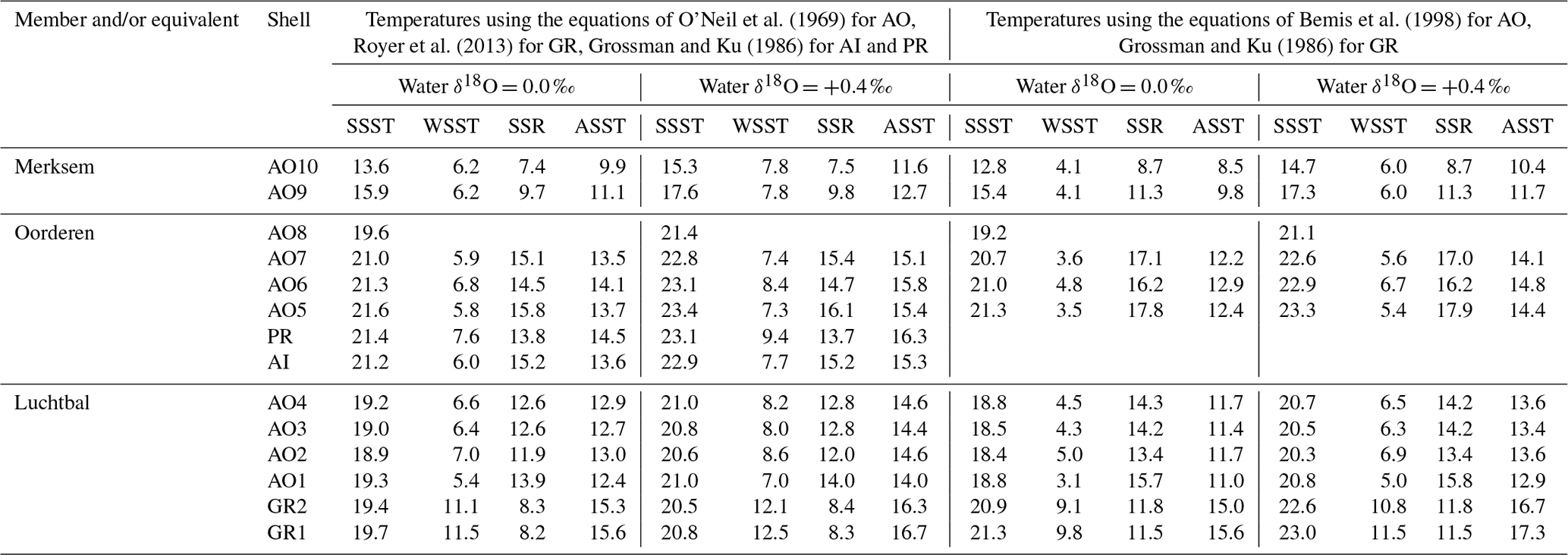
Even if the analysed shells of Luchtbal and Oorderen age were to be from supra- rather than sub-thermocline settings, the δ¹⁸O data from them would specify a seasonal surface temperature range much higher than previously inferred – for example, the majority of shells of Oorderen age indicate a range more than double the 6 ^∘C suggested by organic proxies (see Sect. 6.1.4 and the SFR data in Table 3). We argued in Sect. 2 and Sect. 6.1.2 that seasonal variation in shell δ¹⁸O is unlikely to have been enhanced by variation in water δ¹⁸O, and it can be added here that fluvial input (the means by which variation in water δ¹⁸O might have been brought about) may have been less in the Pliocene than now due to a smaller catchment area of the Rhine–Meuse–Scheldt system (Dearing Crampton-Flood et al., 2020), making enhancement of shell δ¹⁸O variation by water δ¹⁸O variation even more improbable. Notwithstanding these arguments, actual evidence of water δ¹⁸O would be very welcome, both as a check on the stability of values through the year and as a means of deriving accurate absolute temperatures. At present, substitution of independently derived temperatures (e.g. from carbonate clumped isotope or biomineral unit thermometry; Briard et al., 2020; Höche et al., 2020, 2021; Caldarescu et al., 2021; de Winter et al., 2021) into equations relating shell δ¹⁸O to temperature and water δ¹⁸O seems the best approach to determining the last parameter. However, the existence of fluid inclusions in bivalve shell carbonate (Nooitgedacht et al., 2021) raises the possibility that these might serve as a source of direct insight into the isotopic composition of ambient water during life.

It would, of course, also be useful to have additional shell δ¹⁸O (and increment) data, more to confirm the declines in SSST, ASST, and SSR indicated by the limited information from Merksem-age shells than to expand the already substantial evidence of high values for these parameters from shells of Luchtbal and Oorderen age. Notwithstanding some doubts about the reliability of the approach (Johnson et al., 2017), it would also be worth obtaining independent evidence of seasonality from variation in the size of zooids within bryozoan colonies. Using this technique, Knowles et al. (2009, their Table 3) obtained locality-specific seasonality estimates of 8.08±1.38 and 8.15±1.30 ^∘C for the early Pliocene Ramsholt Member of eastern England, figures comparing closely with the estimate of 7.77±1.12 ^∘C obtained through isotope sclerochronology of A. opercularis from this unit (mean difference between the winter and summer seafloor temperatures in Johnson et al., 2021b, their Table 3).

In addition to the above refinements of proxy evidence, further modelling efforts are required to see whether the low winter temperatures indicated by sclerochronological evidence for the mid-Piacenzian SNSB can be reproduced and whether reduced oceanic heat supply is a feasible cause. Haywood et al. (2000) modelled mid-Piacenzian summer surface temperatures 2–4 ^∘C higher than at present for the area, similar to those determined herein. However, they modelled winter temperatures 4–6 ^∘C higher than at present, approaching or into the warm temperate range and markedly above the firmly cool temperate values indicated by sclerochronology. Haywood et al. (2000) ascribed the reduced seasonality specified by their results to greater westerly wind stress and strength in the North Atlantic compared to now, with a resultant increase in heat transport by the Gulf Stream and North Atlantic Current. More recent modelling of mid-Piacenzian seasonal sea surface temperatures at higher northern latitudes indicates greater warming in summer than winter (de Nooijer et al., 2020) – i.e. higher seasonality than now, as inferred for the SNSB. Moreover, as already noted (Sect. 7), oceanic heat supply may not have been greater in the mid-Piacenzian. Possibly, the use of up-to-date models with revised boundary conditions may yield results conforming with the evidence of low winter temperatures and high seasonality from the SNSB.

9 Conclusions

Sclerochronological evidence from bivalves indicates that for most of the late Pliocene (including the MPWP) the seasonal range in surface temperature in the SNSB was higher than now. This was probably a consequence of higher summer temperatures associated with global (atmospheric) warmth. The apparently similar winter temperatures to now may reflect partial withdrawal of oceanic heat supply to the region through a change in strength and/or position of the North Atlantic Current.

Averaging sclerochronologically derived summer and winter temperatures yields an annual sea surface temperature 2–3 ^∘C higher than now in the SNSB, as does averaging temperatures from alkenone and TEX₈₆ thermometry. However, alkenones provide underestimates of extreme summer temperature and TEX₈₆ provides overestimates of extreme winter temperature; hence these proxies do not specify the full seasonal range. The sclerochronologically derived temperatures are based on shell δ¹⁸O and dependent on estimates of water δ¹⁸O that require testing. Back-calculation from temperatures obtained by carbonate clumped isotope or biomineral unit thermometry from the same shells constitutes a potential means.