the Creative Commons Attribution 4.0 License.
the Creative Commons Attribution 4.0 License.
 | 13 May 2022
Calendar effects on surface air temperature and precipitation based on model-ensemble equilibrium and transient simulations from PMIP4 and PACMEDY
Xiaoxu Shi
Martin Werner
Carolin Krug
Chris M. Brierley
Anni Zhao
Endurance Igbinosa
Pascale Braconnot
Esther Brady
Jian Cao
Roberta D'Agostino
Johann Jungclaus
Xingxing Liu
Bette Otto-Bliesner
Dmitry Sidorenko
Robert Tomas
Evgeny M. Volodin
Hu Yang
Qiong Zhang
Weipeng Zheng
Gerrit Lohmann
Numerical modeling enables a comprehensive understanding not only of the Earth's system today, but also of the past. To date, a significant amount of time and effort has been devoted to paleoclimate modeling and analysis, which involves the latest and most advanced Paleoclimate Modelling Intercomparison Project phase 4 (PMIP4). The definition of seasonality, which is influenced by slow variations in the Earth's orbital parameters, plays a key role in determining the calculated seasonal cycle of the climate. In contrast to the classical calendar used today, where the lengths of the months and seasons are fixed, the angular calendar calculates the lengths of the months and seasons according to a fixed number of degrees along the Earth's orbit. When comparing simulation results for different time intervals, it is essential to account for the angular calendar to ensure that the data for comparison are from the same position along the Earth's orbit. Most models use the classical calendar, which can lead to strong distortions of the monthly and seasonal values, especially for the climate of the past. Here, by analyzing daily outputs from multiple PMIP4 model simulations, we examine calendar effects on surface air temperature and precipitation under mid-Holocene, Last Interglacial, and pre-industrial climate conditions. We came to the following conclusions. (a) The largest cooling bias occurs in boreal autumn when the classical calendar is applied for the mid-Holocene and Last Interglacial, due to the fact that the vernal equinox is fixed on 21 March. (b) The sign of the temperature anomalies between the Last Interglacial and pre-industrial in boreal autumn can be reversed after the switch from the classical to angular calendar, particularly over the Northern Hemisphere continents. (c) Precipitation over West Africa is overestimated in boreal summer and underestimated in boreal autumn when the classical seasonal cycle is applied. (d) Finally, month-length adjusted values for surface air temperature and precipitation are very similar to the day-length adjusted values, and therefore correcting the calendar based on the monthly model results can largely reduce the artificial bias. In addition, we examine the calendar effects in three transient simulations for 6–0 ka by AWI-ESM, MPI-ESM, and IPSL-CM. We find significant discrepancies between adjusted and unadjusted temperature values over continents for both hemispheres in boreal autumn, while for other seasons the deviations are relatively small. A drying bias can be found in the summer monsoon precipitation in Africa (in the classical calendar), whereby the magnitude of bias becomes smaller over time. Overall, our study underlines the importance of the application of calendar transformation in the analysis of climate simulations. Neglecting the calendar effects could lead to a profound artificial distortion of the calculated seasonal cycle of surface air temperature and precipitation.
- Article
(28998 KB) - Full-text XML
-
Supplement
(40983 KB) - BibTeX
- EndNote


Long-term fluctuations exist in the Earth's orbital elements that affect the amount of solar radiation received by our planet (Berger, 1978). There are three parameters controlling the motion of the Earth: eccentricity, obliquity, and precession. The shape of the Earth's orbit varies over time from nearly circular with a small eccentricity of 0.0034 to slightly elliptical (large eccentricity of 0.058) with major periodicities of about 400 000 and 100 000 years (Berger, 1978; Berger and Loutre, 1991). When the eccentricity is large, there is also a big difference between the perihelion distance and the aphelion distance, while at a small eccentricity when the orbit is more circular this difference is less pronounced. Earth's orbital eccentricity is 0.016764, 0.018682, and 0.039378 in pre-industrial (1850 CE), mid-Holocene (MH, about 6 ka), and Last Interglacial (LIG, about 127 ka) periods respectively. The seasons are caused by the tilt of the Earth's axis, which is called obliquity. Boreal summer occurs when the Earth's North Pole is tilted toward the sun, and vice versa when boreal winter prevails. Earth's axial obliquity oscillates between 22.1 and 24.5∘ with a major period of 41 000 years. A high obliquity results in stronger seasonal cycles than a low obliquity does. At the same time, the wobble of Earth's rotational axis (precession) modifies the direction of the Earth's tilt and determines which hemisphere is tilted towards the sun at perihelion. The major periodicities of climatic precession are around 19 000 and 23 000 years (Berger, 1978). Precession determines the beginning of each season relative to Earth's orbit and therefore has a major impact on the seasonal pattern of solar radiation. Understanding the role of the three elements of Earth's orbit can help us better examine and interpret past climates from seasonal to millennial timescales.
Numerical modeling of the past climate, which is very different from today, can in many aspects improve our understanding of the underlying mechanisms of the Earth's system and help us better predict the future climate. The Paleoclimate Model Intercomparison Project (PMIP) brings together a number of modeling groups, providing the ability to synchronize results from different models (Kageyama et al., 2018, 2021a).
Two interglacial episodes, i.e., the mid-Holocene (a period roughly from 7 to 5 ka BP) and the Last Interglacial (roughly equivalent to 130–115 ka BP), are particularly the focus of PMIP (Otto-Bliesner et al., 2017), as they are the two most recent warm periods in geological history. So far, there are a variety of previous studies aiming to examine the simulated climate of the mid-Holocene and Last Interglacial. Due to the Earth's orbital parameter anomalies with respect to the present, the MH and LIG receive more insolation in boreal summer and less in boreal winter over the Northern Hemisphere, leading to a larger seasonal temperature contrast in the two time periods (Kukla et al., 2002; Shi and Lohmann, 2016; Shi et al., 2020; Zhang et al., 2021; Kageyama et al., 2021b; Herold et al., 2012; Nikolova et al., 2013). Such an effect is much more profound in the LIG than in the MH (Lunt et al., 2013; Pfeiffer and Lohmann, 2016). In addition, a reduced seasonality in surface air temperature over the Southern Hemisphere continents is simulated (Shi et al., 2020; Nikolova et al., 2013). Climate models identified a northward shift of the Intertropical Convergence Zone (ITCZ) during the two periods, accompanied by a northward displacement of the Northern Hemisphere monsoon domains (Jiang et al., 2015; Braconnot et al., 2007; Nikolova et al., 2013; Fischer and Jungclaus, 2010; Herold et al., 2012). The precession of the MH and LIG, which determines the length of each season, was also different from today. Following the orbital definition of seasons, this results in a calendar (hereafter referred to as the angular calendar) that is different from today's calendar (hereafter referred to as the classical calendar). It has been pointed out in Joussaume and Braconnot (1997) that significant biases occur when we apply today's classical calendar to the MH and LIG seasonal cycles. Therefore, it is important to consider the orbital configuration when defining seasonal cycles for past climate. However, the calendar effect has been investigated in only a few paleoclimate studies. Differences of seasonal ensemble anomalies (LIG minus PI) based on the angular and the classical calendars have been shown by Scussolini et al. (2019) for both precipitation and surface air temperature. Their results indicated pronounced artificial bias for the classical calendar definition: the Northern Hemisphere warming (LIG minus PI) in boreal summer is largely underestimated. Moreover, the Northern Hemisphere monsoon precipitation during the LIG is overestimated in boreal summer but underestimated in boreal autumn. These results are in line with the findings of Joussaume and Braconnot (1997). A recent study by Bartlein and Shafer (2019) examined the “pure” responses of temperature and precipitation to calendar conversion; this was accomplished by applying angular calendars of 6, 97, 116, and 127 ka in a modern climate state. Our present study differs from Bartlein and Shafer (2019) in the following aspects. (1) We use daily data instead of monthly data, so a more accurate result is guaranteed. (2) We perform calendar correction for the pre-industrial period as well, as today's Gregorian calendar is not an angular one. It should be noted that in most previous studies today's calendar has been left unchanged (Joussaume and Braconnot, 1997; Bartlein and Shafer, 2019). (3) In Bartlein and Shafer (2019), the “pure” calendar effects have been examined by applying the angular calendar of 6, 97, 116, and 127 ka onto modern observations. In the present study, we perform a calendar adjustment based on the actual past time intervals of the different model experiments. In detail, we apply an angular calendar of 0, 6, and 127 ka for the pre-industrial, mid-Holocene, and Last Interglacial simulation respectively.
In the present study, we use the PMIP4 dataset to investigate the calendar effect on the simulated surface air temperatures and precipitation under MH and LIG boundary conditions. The structure of the paper is as follows. In Sect. 2, we describe the method for defining an angular calendar based on the Earth's orbital parameters and provide detailed information on the data we used. In Sect. 3 we first briefly describe the main features of simulated MH and LIG surface air temperatures and precipitation, and then we illustrate the effects of the angular season definition on the simulated patterns. We discuss and conclude in Sects. 4 and 5, respectively.
2.1 Calendar correction
In order to appropriately compare the seasonal climate between different time periods resonating with the respective orbital configuration, the seasonality should be calculated according to the position of the Earth along its orbit. First, we define the true anomaly θ as the angle between the axis of the perihelion and the actual position of the Earth. Note that the term “anomaly”, standing for “angle”, is used in astronomy to describe planetary positions. We then define a month (season) as a 30∘ (90∘) increment of the true anomaly, integrated from a fixed starting point. The vernal equinox (VE) is set as 21 March at noon. In the following, we compute the length of a month (season) by calculating how much time the Earth needs to move from the respective starting point to the endpoint. For this purpose, we derive the relation between the true anomaly of any given time and the time elapsed since the Earth passes perihelion.
We define the mean anomaly M as the angle between the perihelion and Earth's position based on the assumption that the orbit describes a perfect circle with the sun at the center by
Here, tp denotes the time elapsed since Earth passes the perihelion, and T is the Earth's revolution period (i.e., 1 year or 365 d), namely the time it takes the Earth to make one complete revolution around the sun. Taking into account the orbit's eccentricity ϵ, we define the eccentric anomaly E via
Equation (2) is called Kepler's equation and is based on Kepler's first and second laws (Fig. S1 in the Supplement). The first law simply states that the orbit of a planet is an ellipse with the Sun at one of the two focus points, and Kepler's second law states that a line segment connecting the sun and a planet sweeps out equal areas during equal intervals of time. Equation (2) can be solved with the application of Newton's method. For more detailed information we refer to Danby and Burkardt (1983). E can be found using the following expression (Eq. 3.13b of Curtis, 2014):
The above equations implicitly relates tp to θ by
Note that E is defined in Eq. (3).
The relation between the true anomaly θ and the time elapsed since Earth passes perihelion tp allows seasons to be defined with respect to Earth's position on the orbit rather than relying on a fixed number of days. Based on the “fixed-angular” approach, there are two ways to define the seasons. (1) The orbit is distinguished into four segments: a true anomaly of θ=0∘ corresponds to 21 March and therefore marks the first day of boreal spring. The length of the boreal summer is gained by calculating tp (θ=90∘). Similarly, the terms tp (θ=180∘) and tp (θ=270∘) mark the beginning of boreal fall and winter, respectively. (2) The other method is based on the “meteorological” definition, in which the boreal spring is defined as March–April–May, as typically done in paleoclimate modeling, although the VE is set to 21 March. The second approach is adopted in our study, and in this case, we first compute the starting and end time for each month and then average over the respective months in order to compare the angular seasonal means with the classical seasonal means. Months can be defined as 30∘ increments of the true anomaly. Just one additional step has to be executed before calculating angular months: as no months start at the VE, the starting day has to be shifted from 21 March to 1 April. Since the time between today's 21 March and 1 April may not be true for past calendars, we defined 1 April by the angle. Therefore, we first calculate the angle between today's 21 March at noon (the VE) and the point of time occurring 10.5 d later, denoting 1 April. Finally, starting from the angle corresponding to 1 April, we are able to calculate the starting time of the next month by 30∘ increments of the true anomaly. Here we apply the so-called “largest remainder method”: the number of days defined by the 30∘ of true longitude usually consists of an integer part plus a fractional remainder. Each month is firstly allocated a number of days equal to its respective integer part (for example, if January has 31.76 d, 31 d are allocated). This generally leaves some days unallocated. The months are then ranked according to their fractional remainders, then an additional day is allocated to each of the months with the largest remainders until all days have been allocated.
The calendar correction method can only be suitably applied on daily data. If only monthly data are available, an alternative option is to reconstruct the daily time series in a way that original monthly mean averages are preserved and then to perform calendar conversion based on the reconstructed daily time series. The mean preserving algorithm is presented in Rymes and Myers (2001).
2.2 Data
We collect the PMIP4 models which provide daily outputs of surface air temperature and precipitation for equilibrium simulations of pre-industrial, mid-Holocene, and Last Interglacial periods. There are nine models that meet the requirement, and we list the detailed information of those models in Table 1.
Sidorenko et al. (2015)Rackow et al. (2018)Sidorenko et al. (2019)Gettelman et al. (2019)He et al. (2019)Li et al. (2020)Volodin et al. (2018)Lurton et al. (2020)Cao et al. (2018)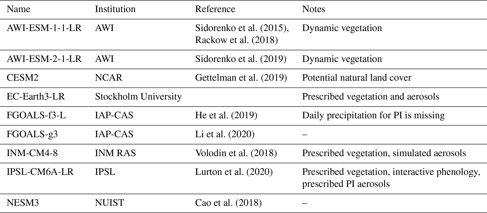
According to Otto-Bliesner et al. (2017), the CO2 concentration applied in the PMIP4 protocol for the mid-Holocene is derived from ice-core measurements from Dome C (Monnin et al., 2001; Monnin et al., 2004). CH4 has been derived from multiple Antarctic ice cores including EPICA Dome C (Flückiger et al., 2002), EPICA Dronning Maud Land (EPICA Community Members, 2006) and Talos Dome (Buiron et al., 2011). The N2O data around 6 ka are compiled from EPICA Dome C (Flückiger et al., 2002; Spahni et al., 2005) and Greenland ice cores. The concentrations of CO2 during the LIG are derived from Antarctic ice cores (Bereiter et al., 2015; Schneider et al., 2013), CH4 has been derived from EPICA Dome C and EPICA Dronning Maud Land (Loulergue et al., 2008; Schilt et al., 2010b), and N2O from EPICA Dome C and Talos Dome (Schilt et al., 2010b, a). The orbital parameters are calculated according to Berger (1978). Table 2 provides a summary of PMIP4 boundary conditions for pre-industrial, mid-Holocene, and Last Interglacial periods.
Table 2PMIP4 boundary conditions for pre-industrial, mid-Holocene, and Last Interglacial periods.

Besides equilibrium simulations, we also use the monthly surface air temperature and precipitation from three transient simulations for the past 6000 years, based on the Earth system models AWI-ESM, MPI-ESM, and IPSL-CM. Using AWI-ESM, we firstly conducted a 1000-year mid-Holocene simulation with dynamic vegetation which was used as initial conditions for the transient experiment. We then conducted the 6–0 ka transient experiment, by applying the boundary conditions of the past 6000 years with the last year representing 1950 CE. Orbital parameters are calculated according to Berger (1977), and the greenhouse gases are taken from ice-core records and from recent measurements of firn air and atmospheric samples (Köhler et al., 2017). The transient simulation performed by MPI-ESM spans the period from 6000 BP until 1850 CE and was initialized from a previous mid-Holocene equilibrium simulation. The model is forced by prescribed orbitally induced variations in the insolation following Berger (1977). CO2, CH4, and N2O forcings stem from ice-core reconstructions (Brovkin et al., 2019). The model accounts for dynamic vegetation changes in the land-surface model JSBACH. A more detailed description of the boundary conditions and the forcing of the transient simulation are given in Bader et al. (2020). The IPSL-CM transient simulation was initialized from a 1000-year mid-Holocene spin-up run. The Earth's orbital parameters are derived from Berger (1977), the concentrations of the trace gases (CO2, CH4, and N2O) are set based on reconstruction from ice core data (Joos and Spahni, 2008), and the vegetation was calculated interactively within the model. More detailed information about the IPSL-CM transient simulation can be found in Braconnot et al. (2019). Therefore, in the transient simulations, the orbital forcings used at 6 and 0 ka are the same as the PMIP4 equilibrium simulations. However, there are differences between the greenhouse gas concentrations applied in the transient and PMIP4 equilibrium simulations, as the values have been taken from different reconstructions.
3.1 Climate responses to the MH and LIG boundary conditions under the classical calendar
Owing to the altered orbital parameters, the MH receives more (less) incoming solar radiation over the Northern Hemisphere during boreal summer (winter) than present (Fig. S2a). As a consequence, the MH Northern Hemisphere experiences a cooling (up to −2 K) and warming (up to 2.5 K) in DJF and JJA respectively (Fig. S3a, b). For the annual average, our model ensemble reveals a general cooling (Fig. S3c) over the Northern Hemisphere, which seems to be inconsistent with the increased annual mean insolation forcing. This phenomenon can be explained by the decreased concentration of greenhouse gases in the MH as compared to present-day condition, which leads to an effective radiative forcing of about −0.3 W m−2, as estimated by Otto-Bliesner et al. (2017).
Regarding the Southern Hemisphere we observe a general cooling in DJF (Fig. S3a), dominated by the decreased insolation in January and February (Fig. S2a). The warming across the Southern Ocean is due to a delayed effect of the increased solar energy in SON. Due to the large heat capacity of water, the ocean responds much more slowly to changes in incoming insolation than the land. Therefore, changes in solar radiation and surface air temperature over the oceans are out of phase. During the MH, the Southern Hemisphere receives more radiation flux in SON relative to the present day, leading to a warming of the Southern Ocean in DJF. Moreover, the models present a robust cooling over most regions of the Southern Hemisphere in JJA, which is mainly led by the reduction in greenhouse gases, as the difference in the incoming solar radiation between the MH and PI is negligible.
The changes in surface air temperature in the LIG with respect to the PI, as shown in Fig. S3d–f, are much more pronounced than those between the MH and the PI. The most intriguing feature is an enhancement in seasonality during the LIG, with a DJF cooling being up to −5 K (over northern Africa and South Asia), as well as a JJA warming (more than 5 K) over North America and Eurasia. This is mostly contributed by the corresponding anomalies in solar insolation (Fig. S2c). In addition, the model-ensemble produces a cooling over the Sahel region as a response to the intensification in monsoonal rainfall. For the Southern Hemisphere, the subtropical continents also experience a DJF cooling and JJA warming (more then 2 K) as responses to the altered incoming solar radiation. Such a feature is robust across the models.
The summer monsoon precipitation is shown to be enhanced over the Northern Hemisphere monsoon domains, in both MH and LIG as compared to modern condition (Fig. S3g–l), driven by the changes in seasonal insolation and the northward displacement of the Inter-Tropical Convergence Zone (ITCZ). The monsoon domain in northern Africa, as well as South Asia, expands significantly in the LIG relative to PI, associated with a stronger land–sea thermal contrast, and an intensification of moisture transport during monsoon seasons. Our results in terms of the responses of the surface air temperature and precipitation to the MH and LIG boundary conditions are in good agreement with the results from the full PMIP4 ensemble as described in Brierley et al. (2020), Otto-Bliesner et al. (2021), and Scussolini et al. (2019), as well as the studies of earlier PMIP ensemble simulations (Lunt et al., 2013).
3.2 Shifts in months/seasons between classical and angular calendars
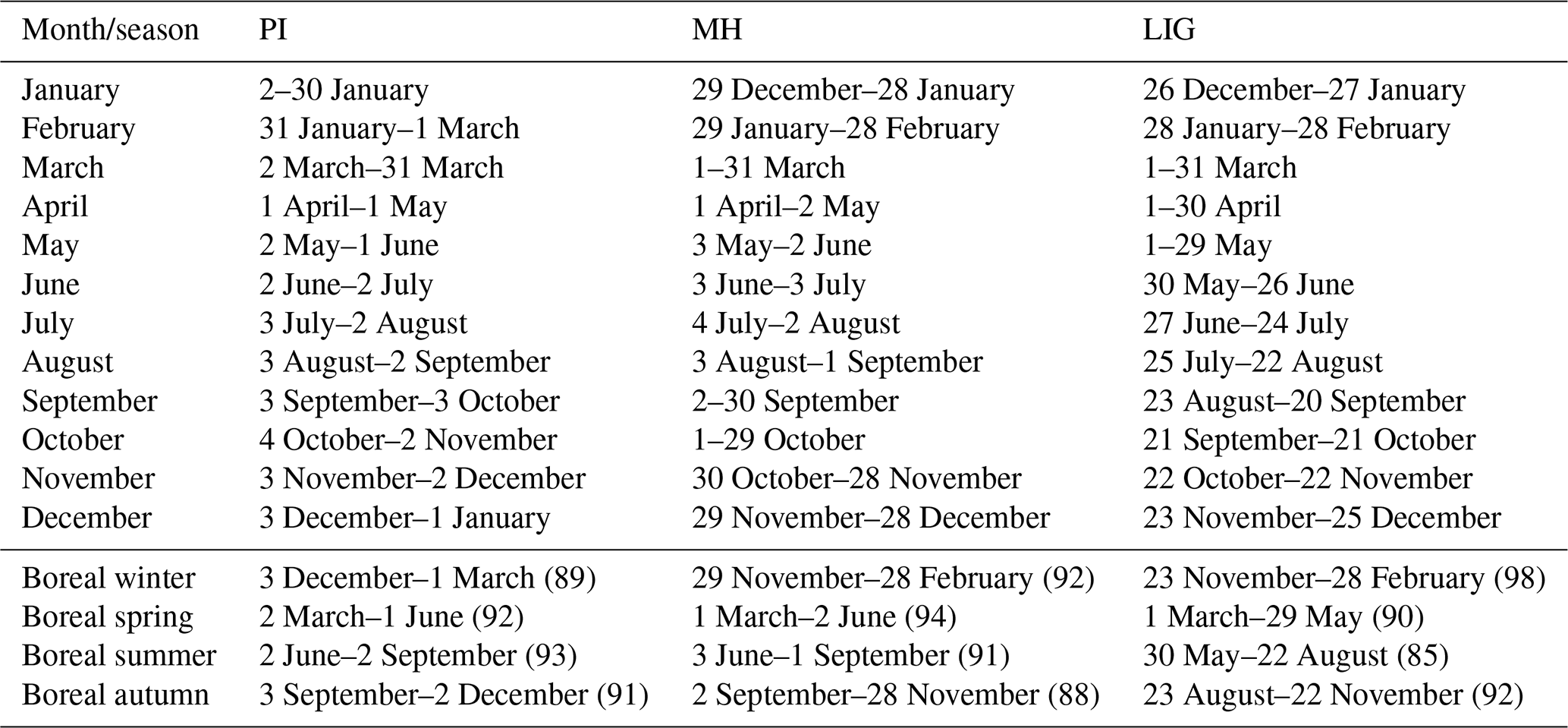
The calculated duration of the angular months and seasons is shown in Table 3. For PI, the shifts in the beginning of most months between the classical and angular calendar are generally in the range of −1 to 2 d, with the exception of October with a 3 d shift. So for today the two approaches are similar. Since the orbital velocity of the Earth is greater at perihelion than at aphelion, the seasons at aphelion are longer than at perihelion; for example for the present-day we have fewer days in boreal winter and more days in boreal summer, which is reflected both in today's classical calendar (DJF: 90 d; JJA: 92 d) and in the angular calendar (DJF: 89 d; JJA: 93 d). The shifts of months for MH are in the range of −2 to 3 d, and the largest shift occurs mainly in the boreal winter. In the MH, boreal winter and spring are longer in the angular calendar than in the classical calendar, while boreal summer and autumn are shorter. Due to the large difference in precession in the LIG compared to today, there are significant shifts in the beginning of the months between classical and angular calendars, especially in boreal autumn (about −10 d). During the LIG, boreal winter has 98 d when the angular calendar is used, which is much longer than boreal summer (85 d).
Table 3Starting and end date of angular month in PI, MH, and LIG, referencing today's classical calendar in a no-leap year, calculated based on the approach described in Sect. 2.1.
3.3 Calendar effects in equilibrium simulations
3.3.1 Surface air temperature
Now we turn to examine the calendar effects on the seasonal cycle of surface air temperature. Figure 1 depicts the differences in seasonal surface air temperature between angular and classical means. Positive (negative) values indicate warming (cooling) in angular-mean temperatures as compared to classical-mean temperatures. We observe spatially variable changes of surface air temperature in adjusted values as compared to unadjusted values. For the LIG, the most pronounced pattern is a warming over the Northern Hemisphere up to 5 K in boreal autumn (SON), as well as a cooling over the Southern Hemisphere especially the Antarctic continent (up to −3 K). This is explicable by the fact that the angular SON receives more (less) insolation over the Northern (Southern) Hemisphere than the classical SON does (Figs. 2a, S2), in agreement with the earlier onset of those months. As the VE is fixed on 21 March, the calendar effect is expected to be relatively minor for boreal spring (MAM). Indeed, we find only a slight increase (within 0.3 K) in the Northern Hemisphere surface air temperature in classical means as compared to angular means, and for the Southern Hemisphere the calendar-adjusted minus unadjusted values are in the range of −0.1 to 0 K, dominated by the pattern in May (Fig. S4). We are aware that there is no difference between adjusted and unadjusted values in March and April, as no shift occurs in the beginning of and during these two months (Table 3). In boreal winter (DJF), the most prominent calendar effects on LIG surface air temperature can be seen over the Northern Hemisphere, with a warming up to 1.5 K, as well as the oceans of the Southern Hemisphere, which experiences a cooling up to −0.4 K. Such a pattern is dominated by the temperature anomalies in December (Fig. S4). The warming signal over Antarctica (0–0.5 K) in DJF is mainly determined by increased insolation during January and February. The conversion of the calendar produces a cooling (within −1 K) over the Northern Hemisphere ocean and Southern Hemisphere continents (except Antarctic) in boreal summer (JJA), while for other regions, especially the Northern Hemisphere continents, we obtain positive anomalies in surface air temperature.
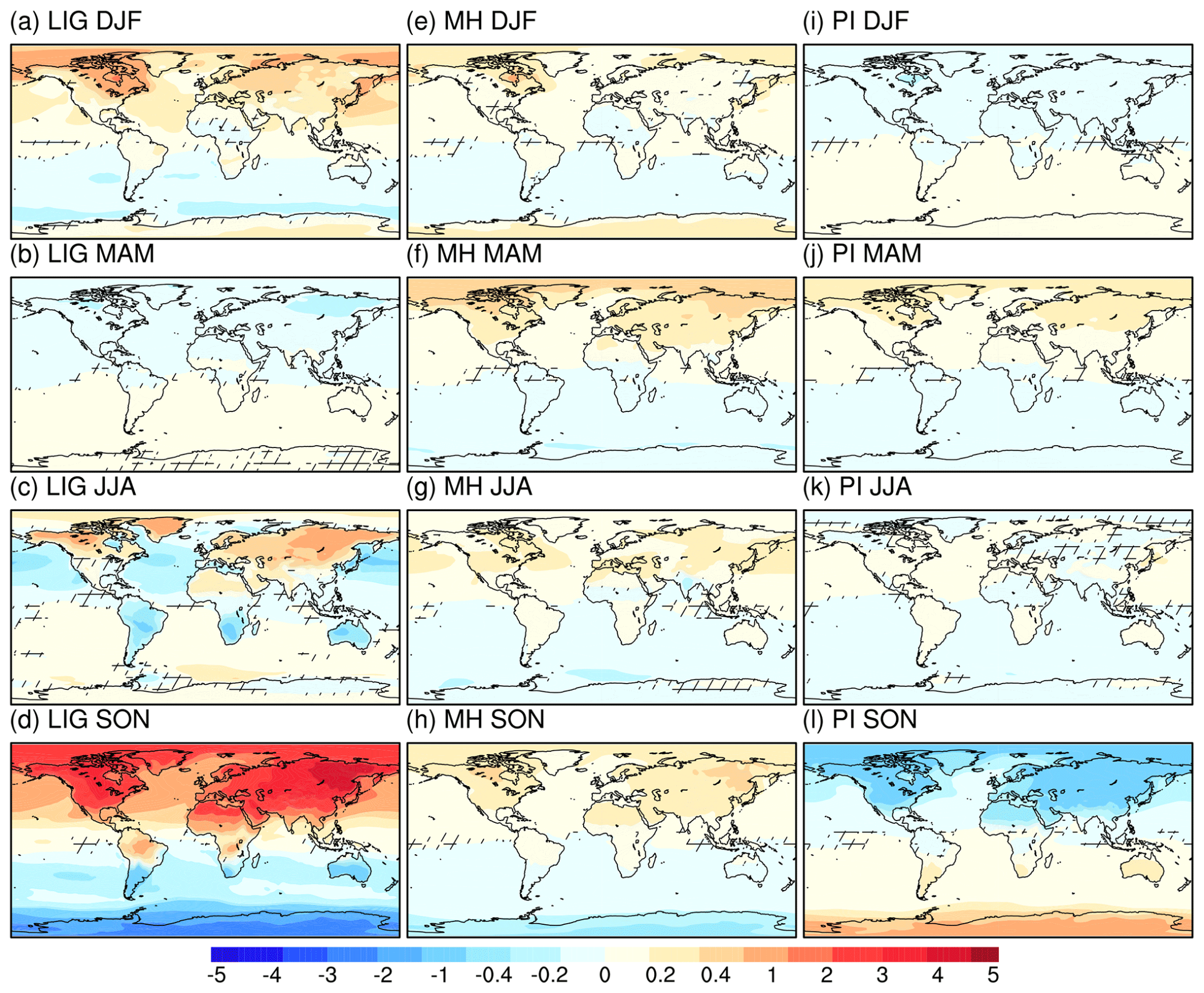
Figure 1Ensemble anomalies of surface air temperature between angular means and classical means. The unmarked area indicates that at least seven models show the same sign. Units: K.
Compared to the LIG, the response of surface air temperature to calendar effect in the MH is less pronounced (Fig. 1). It reveals a dipole pattern in all seasons, with warming over the Northern Hemisphere and cooling over the Southern Hemisphere. One exception is the Antarctica warming in boreal winter, led by the increased insolation in January and February over Antarctica (Fig. 2b). Figure S5 shows the adjusted minus non-adjusted temperatures for each month. No difference is found for March, as for the mid-Holocene the beginning and end of March in the angular calendar are the same as in the modern classical calendar (Table 3). From April to June, the delay in the angular calendar leads to a positive insolation difference and therefore a warming over the Northern Hemisphere, while the opposite is the case for the Southern Hemisphere. Similar patterns are observed for October to November, but this is due to an advance in those months (the peak insolation happens in June). In general, we notice that the temperature anomalies on continents are in phase with the insolation changes, while the calendar effect on surface air temperature over the ocean is delayed due to the large heat capacity of sea water.
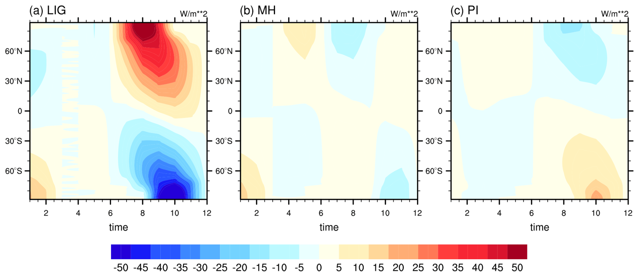
Figure 2Insolation anomalies between angular and classical calendar for (a) LIG, (b) MH, and (c) PI.
For PI, the classical calendar used at present is similar to today's angular calendar from January to June (Table 3), and this leads to relatively minor changes in surface air temperature in boreal winter, spring, and summer (Figs. 1i–k, S6) in angular-mean values as compared to classical-mean values. In boreal autumn, a dipole pattern of insolation anomaly is obvious (Fig. 2c): less (more) insolation is received at the top of the atmosphere over the Northern (Southern) Hemisphere in adjusted SON than that in non-adjusted SON, consistent with the delay of boreal autumn in angular calendar as compared to the classical calendar. Such a pattern favors cooling (up to −0.4 K) over the Northern Hemisphere and warming over the Southern Hemisphere during SON.
Knowing the pure calendar effect on the surface air temperature for the respective time period, now we turn to investigating to what degree the temperature anomalies between paleo and pre-industrial periods can be affected by calendar conversion. As shown by Fig. 3, in boreal winter, spring, and summer, we observe similar patterns for both definitions of seasonal means. The insolation changes induced by changes in orbital parameters produce an enhanced seasonality in LIG as compared to PI, with colder boreal winter and warmer boreal summer, especially over Northern Hemisphere continents. However, with classical calendar applied, the DJF cooling over the Northern Hemisphere is overestimated by up to 1 K, whilst an underestimation in the MAM cooling happen over the Northern Hemisphere, with a magnitude up to 1 K. For JJA, the bias in temperature anomaly, as calculated from classical means, is not uniform and has a clear land–sea contrast. The classical calendar tends to underestimate the JJA warming over Northern Hemisphere lands (by 1 K) and Southern Hemisphere oceans (0.2 K), while the warming over North Atlantic, North Pacific, and Southern Hemisphere continents are overestimated in the classical calendar. The most prominent calendar effect can be seen in SON, as the temperature anomaly over Northern Hemisphere continents in SON flips its sign after switching from classical means to angular means, with the magnitude of the bias being as large as −5 K for classical means. Such an artificial bias could be interpreted as climatic signals without the application of the adjusted calendar.

Figure 3Ensemble surface air temperature for (a–d) LIG minus PI classical means, (e–h) LIG minus PI angular means, and (i–l) anomalies between LIG minus PI angular means and LIG minus PI classical means. The unmarked area indicates that at least seven models show the same sign. Units: K.
For the temperature anomalies between MH and PI as shown in Fig. 4, the most significant bias introduced by the use of the classical calendar occurs in SON over Northern Hemisphere continents (more than 1 K), which appears to be colder in MH as compared to PI for classical means, and warmer for angular means. Moreover, the warming over Antarctica in MH relative to PI is overestimated in the classical calendar. From DJF through MAM, both calendars show a general colder-than-present climate in MH, and the use of the present classical calendar causes a cooling bias (within −0.5 K) for the Northern Hemisphere and Antarctic, as well as a warming bias (within 0.3 K) for the Southern Hemisphere oceans. In boreal summer, the key characteristic shared in both angular and classical means is a warming over the Arctic Ocean, North Atlantic, and Eurasia, led by increased JJA insolation in MH as compared to PI. Such warming is more pronounced in the angular calendar than in the classical calendar.

Figure 4As Fig. 3, but for the MH.
Analysis on individual models reveals a robust calendar effect on SON surface air temperature for both continents and oceans, which overwhelms the differences between models (Fig. 5). We also observe that the calendar effect on temperature anomalies is more pronounced at higher latitudes than at lower latitudes.
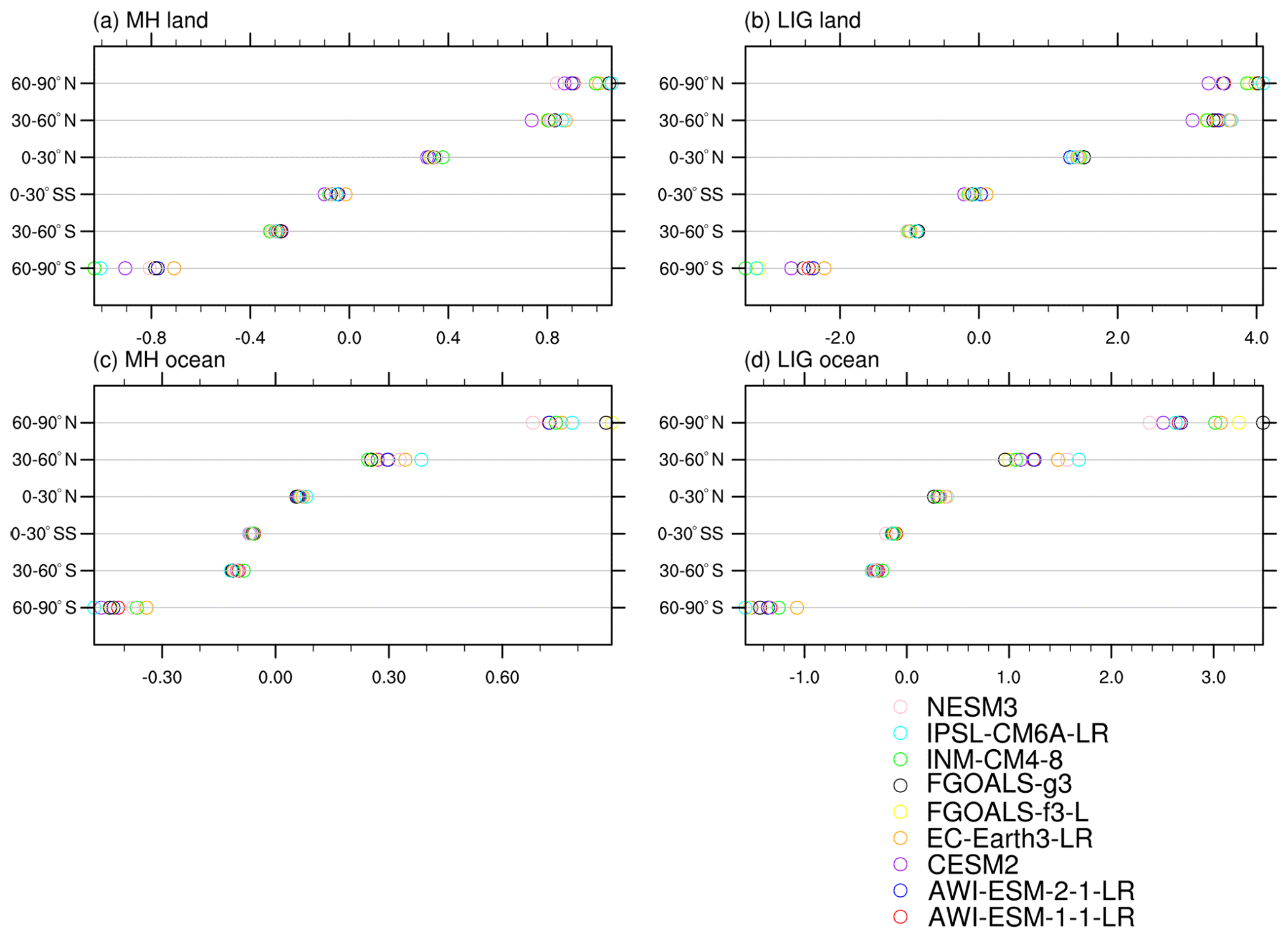
Figure 5(a, b) Deviation of MH-PI SON surface air temperature between angular and classical means for (a) continents and (b) oceans at different latitude bands, simulated by individual models. (c, d) As in (a, b), but for LIG-PI surface air temperature. Units: K.
3.3.2 Precipitation
In LIG, the largest calendar effects on precipitation can be observed for SON over the tropical rain belt (Fig. 6 shows the anomalies and Fig. S7 shows the percentage changes), with positive anomalies (within 30 mm per month) to the north and negative anomalies (up to −30 mm per month) to the south of the Inter Tropical Convergence Zone (ITCZ). In northern Africa, changes in precipitation due to calendar transition account for up to 80 % of the classical mean (Fig. S7d). In DJF, we observe a tripole pattern, with negative anomalies over northern (−1 mm per month, −10 %) and southern Africa (−4 mm per month, −5 %) and positive anomalies over equatorial Africa (5 mm per month, 8 %). For JJA the adjusted-minus-unadjusted precipitation anomalies present a dryness (up to −15 mm per month, −15 %) and wetness (less than 10 mm per month, 16 %) over the northern and southern edge of the ITCZ, respectively, opposite to the patterns for SON and DJF. The calendar effect appears to be small during boreal spring, as the vernal equinox is fixed on 21 March in both calendars. In contrast to the calendar-induced significant changes in large-scale patterns of LIG precipitation, the effect of calendar on MH precipitation is much less pronounced, showing positive (negative) anomalies up to 5 (−5) mm per month over the north (south) branch of the tropical rain belt for all seasons. This is associated with the di-pole pattern of temperature differences between angular and classical means (warming over Northern Hemisphere and cooling over Southern Hemisphere). For PI, a northward displacement of ITCZ is obvious during SON for angular-mean as compared to classical-mean precipitation, while, for other seasons, no pronounced changes in precipitation can be observed.
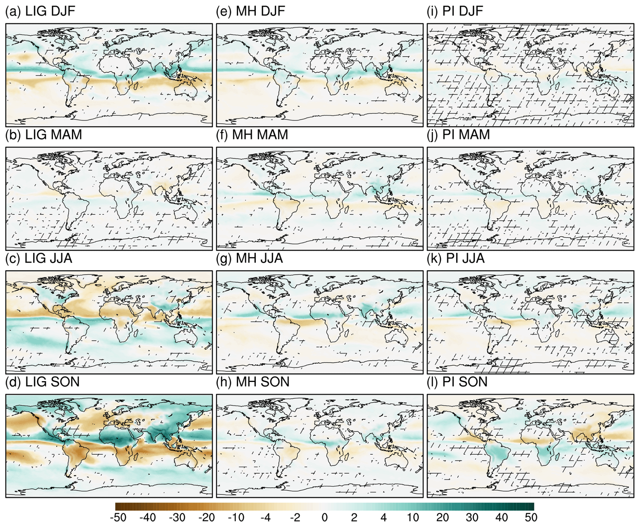
Figure 6Ensemble anomalies of precipitation between angular and classical means for (a–d) LIG, (e–h) MH, and (i–l) PI. The unmarked area indicates that at least seven models show the same sign. Units: mm per month.
The anomalies in precipitation (LIG-PI), as well as the impact of calendar conversion on the precipitation anomalies, are shown in Fig. 7. The general patterns of precipitation anomalies (LIG-PI) are very similar for both angular and classical means, revealing a northward shift of the ITCZ especially from JJA through SON, evidenced in the wetter conditions to the north of ITCZ and the drier conditions to the south. Such a pattern is overestimated in JJA and underestimated in SON when the present classical calendar is applied. For both calendars, MH also presents a similar distribution in precipitation anomalies as for LIG, with a much smaller magnitude (Fig. 8). Moreover, the application of the classical calendar leads to an underestimation of the increased summer monsoon rainfall in MH as compared to PI over the Northern Hemisphere monsoon domains, i.e., West Africa, North America, and South Asia.
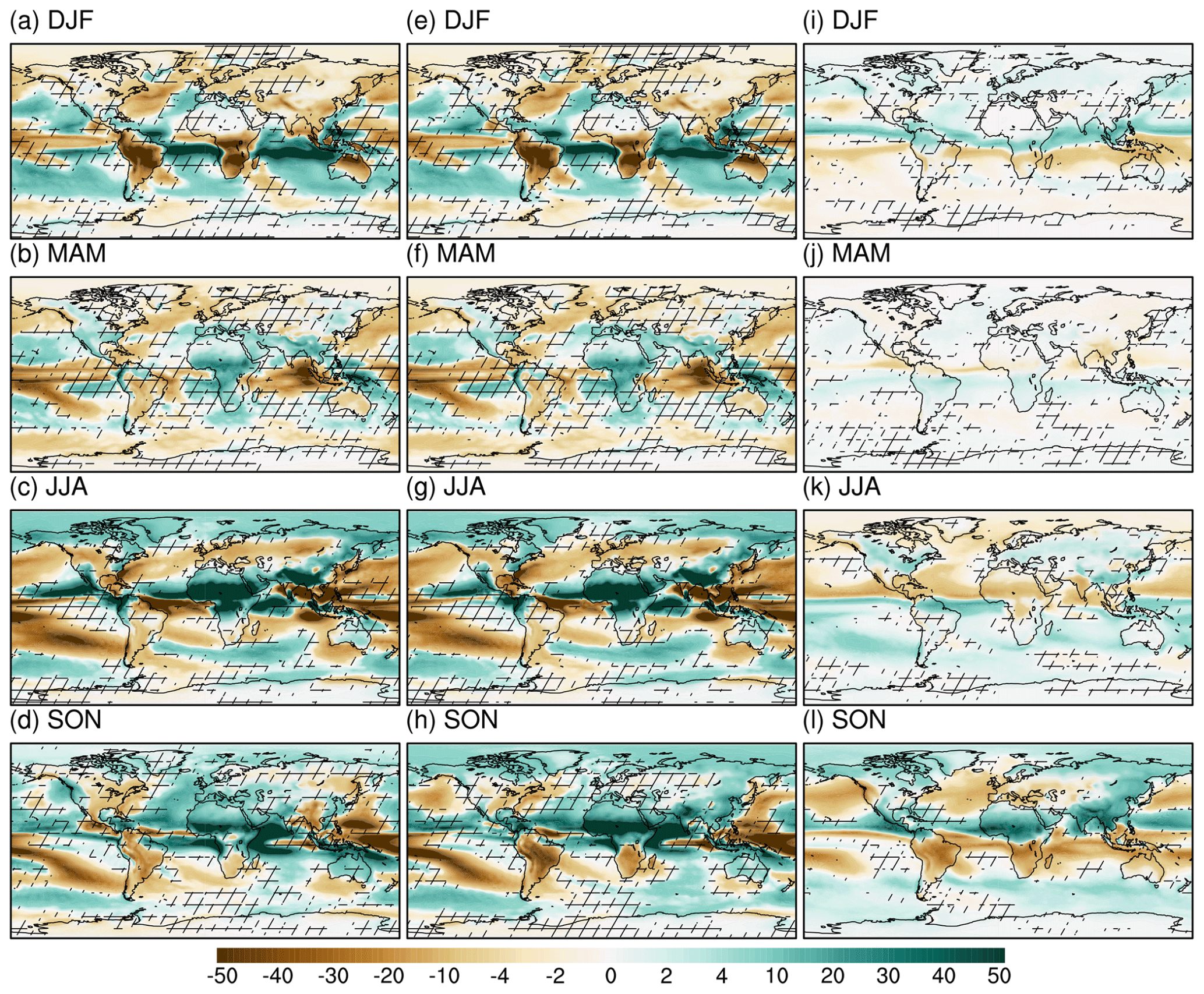
Figure 7Ensemble precipitation for (a–d) LIG minus PI classical means, (e–h) LIG minus PI angular means, and (i–l) anomalies between LIG minus PI classical means and LIG minus PI angular means. The unmarked area indicates that at least seven models show the same sign. Units: mm per month.
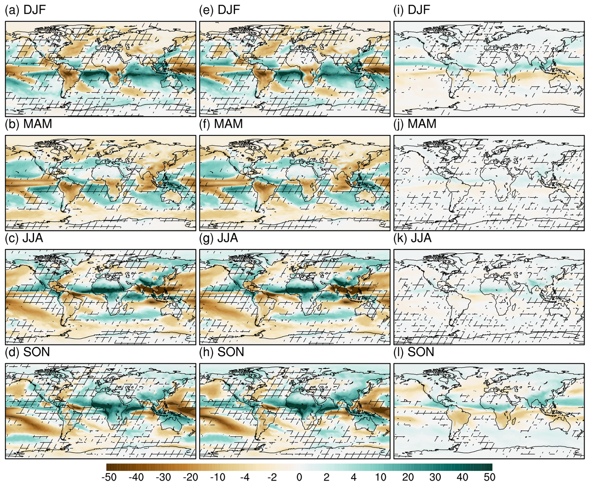
Figure 8As Fig. 7, but for the MH.
Figure 9 depicts the calendar impact on the SON precipitation anomaly over the main monsoon domains of the Northern Hemisphere (i.e., North America, northern Africa, and South Asia). We notice a very large model–model discrepancy for all regions examined in both the MH and the LIG, with the exception of northern Africa in the MH. Our results indicate that during the MH, the precipitation in South Asia is more responsive to a calendar adjustment compared to northern Africa and North America. However, for the LIG, no robust conclusion could be drawn about the calendar effects in the different regions due to the large discrepancies between the models.
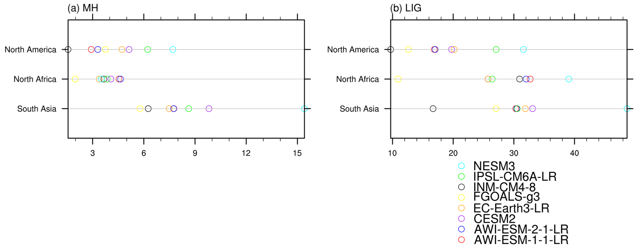
Figure 9(a) Deviation of SON MH-PI precipitation between angular and classical means for North America, northern Africa, and South Asia, simulated by individual models. (b) As in (a), but for LIG-PI precipitation. Units: mm per month.
Overall, it is crucial to perform calendar conversion before examining the surface temperature and precipitation differences between LIG/MH and PI, as non-ignorable artificial bias can be introduced to the seasonal cycle of temperature and precipitation with the application of the present classical calendar, which could be misinterpreted as climatic feedbacks.
3.3.3 Calendar conversion based on monthly data
Daily output takes up much more space than monthly output, so most modeling groups only provide monthly frequency variables. Here, we utilize a calendar transformation method that requires only the raw (i.e., classical calendar) monthly mean values (Rymes and Myers, 2001). In the study of Rymes and Myers (2001) an approach has been introduced for smoothly interpolating coarsely-resolved data onto a finer resolution, while preserving the deterministic mean. Based on the approach, daily data can be reconstructed using the monthly mean values: the daily data are initialized with the monthly average of the respective month. Then, for each day of the year, its value is recursively recalculated as the average of its own value and the values of the two adjacent days. After 365 iterations, this results in a nicely smooth annual cycle with the original monthly means being preserved. Using this approach, we perform calendar corrections based on the monthly outputs of the same nine modeling groups. We then check the deviation of this month-length adjusted values from the day-length adjusted values. Here the month-length and day-length adjusted values represent the adjusted values after calendar correction based on the original monthly and daily data respectively. From Figs. S8 and S9 we can conclude that the conversion of the calendar based on monthly mean values can improve the seasonal cycle to a large degree. For MH and PI, we observe only a slight bias, with the temperature deviation being less than ±0.05 K and precipitation deviation less than ±1 mm per month, indicating that the calendar transformation based on monthly data can serve as an alternative for seasonal adjustment of MH and PI. We are aware of a slight artificial bias in month-length adjusted surface air temperature for LIG over the high-latitude continents in JJA, which is underestimated by 0.07 K. During boreal autumn, the land is generally cooler and the tropics and Southern Ocean are generally warmer compared to the day-length adjusted values.
As stated above, we find spatial heterogeneity in the response of surface air temperature to calendar conversion across the globe, which is manifested in the opposite signals between two hemispheres and the contrast between land and ocean. Our model ensemble shows that the calendar effect is more pronounced over continents than over seawater areas. Here we calculate the seasonal cycle of surface air temperature for (1) the original daily average, (2) the original monthly average, (3) daily length-adjusted mean values, and (4) month-length adjusted mean values, over different continents, shown in Fig. 10. We find the day-length and month-length adjusted values are very similar, evidenced in the overlapping orange and purple solid lines in Fig. 10. This suggests that the monthly calendar correction approach can serve as a good alternative when only monthly frequency model outputs are available for surface air temperature. For North America and Eurasia, we observe a slight positive anomaly in the PI between adjusted and unadjusted surface temperatures from January to July (less than 0.2 K), while negative anomalies are found from August to December, with the maximum change occurring in October (−0.7 K). For the Antarctic, the greatest calendar effect occurs in October and November, with the mean adjusted-minus-unadjusted value being 0.8 K. This agrees with the spatial maps shown in Fig. S6. For the MH, the calendar effect over North America and Eurasia appears to be greatest in May–June (0.5 K) and October–December (0.6 K). Over the Antarctic continent, apart from the warming in January–February (0.5 K) and the cooling in November (−0.7 K), no significant response of the mean surface air temperature to the calendar conversion was found. In terms of the LIG, the mean adjusted-minus-unadjusted surface air temperature in October reached up to 3 K in both North America and Eurasia. The maximum temperature change in Antarctica also occurs in October, with a magnitude of −3 K. In addition, we calculated the seasonal cycle of precipitation values for the following monsoon domains: North America (5–30∘ N, 120–40∘ W), African monsoon region (5–23.3∘ N, 15∘ W–30∘ E), and South Asia (5–23.3∘ N, 70∘ W–120∘E). As shown in Fig. 11, again we see very similar day-length and month-length adjusted values. Therefore, performing calendar correction based on monthly precipitation can help reduce the artificial distortion of monsoon rains to a large extent. In addition, we also observe some discrepancies between the seasonal cycles based on daily and monthly precipitation. One example is the peak value in July (late June) for MH (LIG) as indicated by the daily rainfall over South Asia, which is not presented in the monthly average. Similar cases can also be found for North America during warm months.
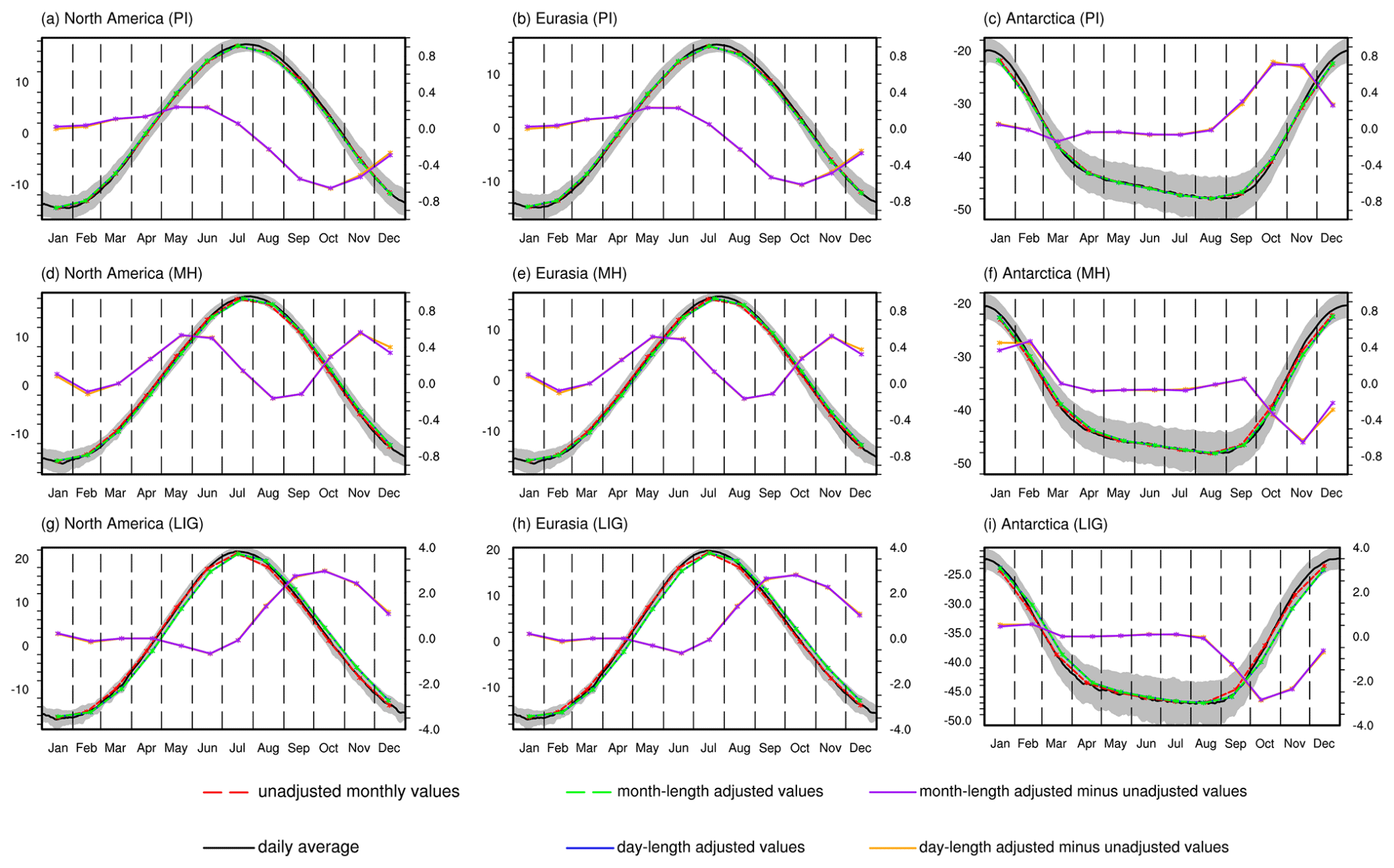
Figure 10Ensemble seasonal cycle of regional mean surface air temperature in daily average (black solid lines), classical monthly means (red dashed lines), day-length adjusted means (blue dashed lines), and month-length adjusted means (green dashed lines) for (a–c) PI, (d–f) MH, and (g–i) LIG (axis to the left). Grey area represents one standard deviation from the multi-model ensemble daily mean values. Purple (orange) solid line represents the month-length (day-length) adjusted minus unadjusted values, axis to the right. The values are calculated by averaging the surface air temperatures over (a, d, g) North America, (b, e, h) Eurasia, and (c, f, i) Antarctica. Units: ∘C.
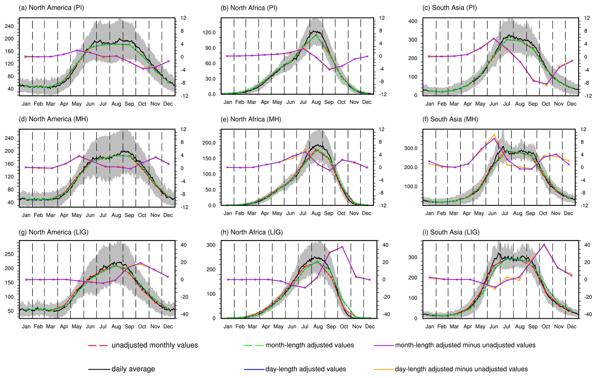
Figure 11Ensemble seasonal cycle of regional mean precipitation in daily average (black solid lines), classical monthly means (red dashed lines), day-length adjusted means (blue dashed lines), and month-length adjusted means (green dashed lines) for (a–c) PI, (d–f) MH, and (g–i) LIG. Grey area represents 1 standard deviation from the multi-model ensemble daily mean values. Purple (orange) solid line represents the month-length (day-length) adjusted minus unadjusted values (axis to the right). The values are calculated by averaging the precipitation over (a, d, g) North America, (b, e, h) northern Africa, and (c, f, i) South Asia. Units: mm per month.
3.4 Calendar effects in transient simulations
Calendar effects should be considered also in the analysis of transient simulations (Bartlein and Shafer, 2019). Here with the utility of three mid-Holocene-to-present transient runs based on AWI-ESM, MPI-ESM, and IPSL-CM respectively, we examine the degree of influence of calendar definition on surface air temperature and precipitation. All the three experiments provide outputs in monthly frequency; therefore we perform calendar transformation based on monthly surface air temperature and precipitation using the approach described by Rymes and Myers (2001).
The time series plotted in Fig. 12 are for adjusted and unadjusted mean surface air temperature over the Northern Hemisphere continents (i.e., Greenland, North America, Eurasia, and northern Africa) for all seasons. Based on all the three models, the largest deviation between angular and classical-mean temperature values happens in boreal autumn between 6 and 4.4 ka, with the temperature being underestimated under the classical calendar. Another distinct difference between month-length adjusted and unadjusted values occurs in boreal autumn between 4.4 and 0 ka. During this time interval, the surface air temperature over Northern Hemisphere continents can be overestimated when using the classical calendar. This phenomenon, again, highlights the importance of calendar correction in the analysis of both mid-Holocene and pre-industrial climates, especially in boreal autumn. Without the calculation of angular seasonality, the warming in the mid-Holocene relative to pre-industrial in SON can be largely underestimated. In DJF, no obvious deviation is found between the angular and classical means, evidenced in the overlapped black and red lines in the top panels of Fig. 12. During boreal spring, all three models reveal a slight cooling bias in the original temperature values throughout the whole integrated time period, which is relatively more manifested in the mid-Holocene and pre-industrial than in 3–1 ka. In JJA, besides the slight cooling bias in the original mean surface air temperature for 6–3 ka as revealed by all three models, we observe a model dependency of the calendar effects for the time interval of 3–0 ka, during which the Northern Hemisphere classical-mean temperature in JJA is slightly underestimated by AWI-ESM and MPI-ESM, but for IPSL-CM the adjust and unadjusted values are identical. Such a discrepancy between models is related to the spatially varying temperature changes over the Northern Hemisphere continents caused by the calendar effect (Fig. 1k). The calendar effect on Northern Hemisphere temperature over oceans, as shown in Fig. 13, is very similar to that over lands. However, the deviation between adjusted and unadjusted SON temperature is much less pronounced. This is also consistent with the results from the equilibrium simulations. Moreover, in JJA, all models show positive anomalies of the angular-minus-classical mean temperature over ocean, with the magnitudes being smaller from 6 to 0 ka.
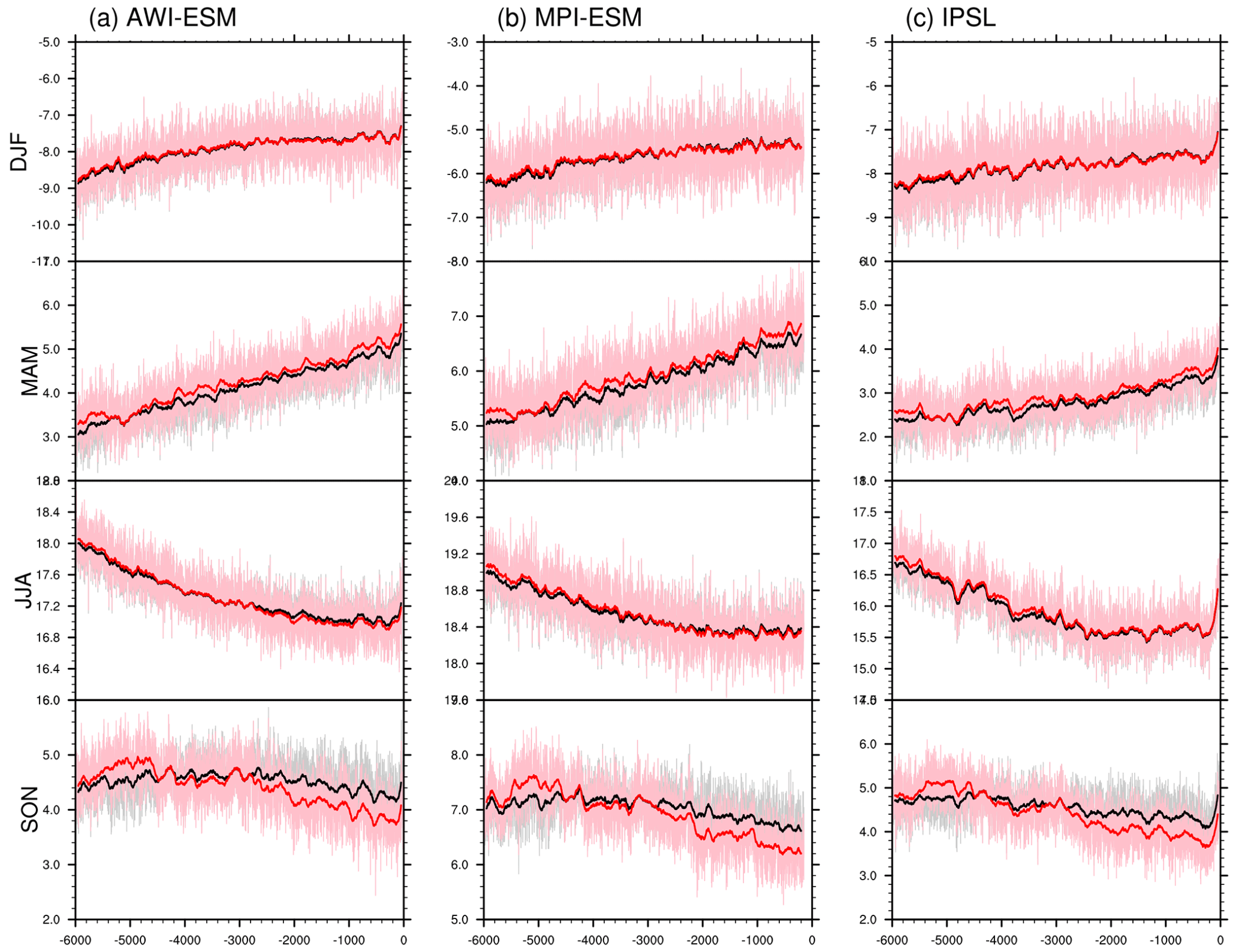
Figure 12Time series of surface air temperature in classical and angular means averaged over Northern Hemisphere continents, weighted by month length, for (a) AWI-ESM, (b) MPI-ESM, and (c) IPSL-CM. Grey and pink lines stand for the original classical and angular means respectively. Smoothed curves with a running window of 100 model years are shown in black (for classical means) and red (for angular means). Units: ∘C.
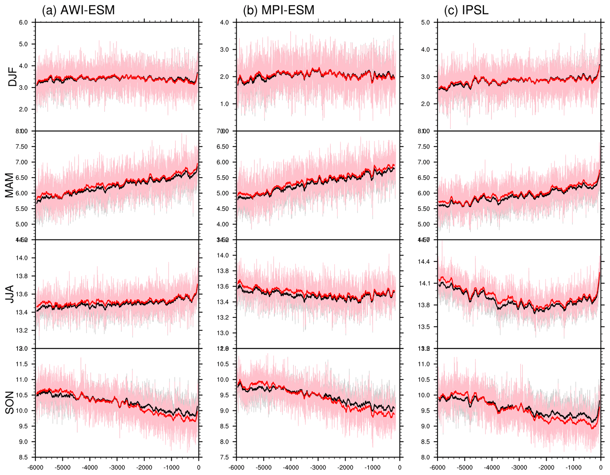
Figure 13Time series of surface air temperature in classical and angular means averaged over Northern Hemisphere oceans, weighted by month length, for (a) AWI-ESM, (b) MPI-ESM, and (c) IPSL-CM. Grey and pink lines stand for the original classical and angular means respectively. Smoothed curves with a running window of 100 model years are shown in black (for classical means) and red (for angular means). Units: ∘C.
For the Southern Hemisphere lands, including South America, Australia, Southern Africa, and Antarctic, as shown in Fig. 14, the calendar effects are less pronounced as compared to Northern Hemisphere. Similar to the Northern Hemisphere, no distinct temperature deviation is seen for DJF. Besides, all the three models agree on the cooling bias in classical-mean temperatures in SON from 4 to 0 ka, as well as a slight warming deviation during MAM (6–0 ka). For JJA, no noticeable change in temperature could be found in IPSL, while the other two models (AWI-ESM and MPI-ESM) reveal a positive anomaly between the adjusted and unadjusted means. The oceans appear to have a more pronounced response to calendar adjustment in boreal autumn (Fig. 15). For other seasons, no obvious deviation of temperature is seen for the Southern Hemisphere oceans.

Figure 14Time series of surface air temperature in classical and angular means averaged over Southern Hemisphere continents, weighted by month length, for (a) AWI-ESM, (b) MPI-ESM, and (c) IPSL-CM. Grey and pink lines stand for the original classical and angular means respectively. Smoothed curves with a running window of 100 model years are shown in black (for classical means) and red (for angular means). Units: ∘C.
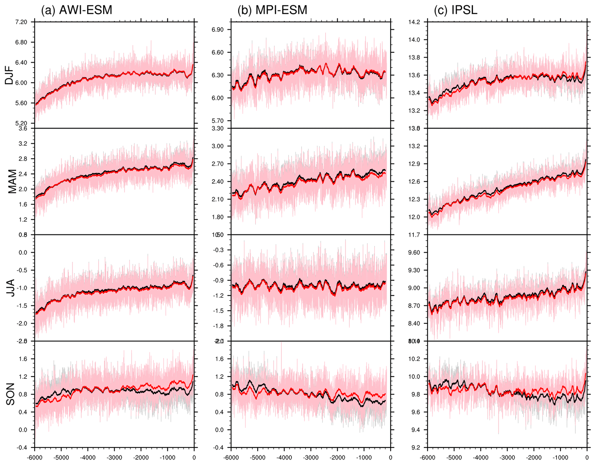
Figure 15Time series of surface air temperature in classical and angular means averaged over Southern Hemisphere oceans, weighted by month length, for (a) AWI-ESM, (b) MPI-ESM, and (c) IPSL-CM. Grey and pink lines stand for the original classical and angular means respectively. Smoothed curves with a running window of 100 model years are shown in black (for classical means) and red (for angular means). Units: ∘C.
Figure S10 illustrated the calendar effects on the African monsoon precipitation. The time series in Fig. S10 are derived by averaging month-length adjusted and unadjusted JJA precipitation over the land points within 5–23.3∘ N, 15∘ W–30∘ E. All three transient simulations show a slight artificial drying bias in the African monsoon precipitation with the application of the classical calendar in 6 ka. It is also shown that such a calendar effect gradually becomes weaker from the mid-Holocene to the present.
Two important elements should be taken into consideration when comparing paleoclimate simulations of different time intervals: the reference date (usually the VE) and the angle of the orbit of the Earth around the Sun, which defines the phasing of the insolation curve. Artificial bias emerges when precessional effects are ignored, and such a bias can be amplified by eccentricity changes (Joussaume and Braconnot, 1997). To avoid such a bias, one shall define the seasonal cycle based on astronomical positions along the elliptical orbits. The sensitivity of simulated paleoclimate conditions to the “classical” and “angular” calendars had been investigated in a former study based on one single coarse-resolution model (Joussaume and Braconnot, 1997), in which the authors state that the differences between the two calendar means cannot be neglected. Here by examining seven of the most advanced climate models in PMIP4, we again confirm the necessity of calendar definition in paleoclimate modeling research.
Daily data are needed for calendar adjustment; however, due to the large volume of daily outputs, they are not preserved by most modeling groups. A mean preserving algorithm has been introduced (Rymes and Myers, 2001), with which the daily time series can be reconstructed. By performing calendar correction on the reconstructed daily time series, we find that the seasonal pattern in temperature and precipitation can be largely ameliorated, even though there is still room for improvement.
Various methods for adjusting monthly data towards an angular calendar have been suggested. Rymes and Myers (2001) developed a mean-preserving running-mean algorithm to reconstruct the annual cycle. In Pollard and Reusch (2002), the reconstruction of an annual cycle was based on a spline method, which fits each monthly segment by a parabola, requiring the same monthly means as the originals and continuity of value and slope at the month boundaries. Bartlein and Shafer (2019) used a mean-preserving harmonic interpolation method described in Epstein (1991) and performed the same function as the parabolic-spline interpolation method as in Pollard and Reusch (2002). To sum up, the basic procedure is similar in all the approaches, as they are all based on “mean-preserving” algorithm. In Bartlein and Shafer (2019), a comparison was made between the linear and mean-preserving interpolation methods. They found that the difference between the original monthly means and the monthly means of the linearly interpolated daily values is not negligible for both surface air temperature and precipitation, while the difference between an original monthly mean value and one calculated using the mean-preserving interpolation method is negligible.
In previous studies, the angular calendar was defined using the true anomaly of the Earth corresponding to the present-day seasons; in other words, each month begins and ends at the same celestial longitude as the present day for any period (Joussaume and Braconnot, 1997; Bartlein and Shafer, 2019; Timm et al., 2008; Chen et al., 2011; Pollard and Reusch, 2002). The work of Chen et al. (2011) and Timm et al. (2008) applied a 360 d year which is, originally, divided into 12 months with 30 d. The VE is set to day 81 in a calendar year. Pollard and Reusch (2002), Joussaume and Braconnot (1997) and Bartlein and Shafer (2019), on the other hand, performed the calendar adjustment based on today's classical calendar with 365 d in a non-leap year. In their studies, an assumption was made that the seasonality defined by the classical calendar is in phase with the insolation and solar geometry for the modern day. In our study, by calculating the onset of present-day months/seasons using the approach described in Sect. 2.1, we find that the classical calendar is very similar to the angular calendar for today, but they are not completely the same. This is evidenced in the small shift of months between the two calendars as seen in Table 3. In particular the angular October is delayed by 3 d compared to the classical October, resulting in negative anomalies in the adjusted-minus-unadjusted solar insolation. Though different methods are used in our work from the mentioned previous studies, our results are identical: for the LIG, the adjusted-minus-unadjusted surface air temperature over the Northern Hemisphere is up to 5 K during SON (Joussaume and Braconnot, 1997; Bartlein and Shafer, 2019; Chen et al., 2011) or September (Pollard and Reusch, 2002); and the Northern Hemisphere monsoon precipitation in SON is underestimated by the use of the classical calendar (Bartlein and Shafer, 2019; Chen et al., 2011). Similar biases are found for the early Holocene (Timm et al., 2008) and mid-Holocene (Joussaume and Braconnot, 1997; Bartlein and Shafer, 2019) but are less pronounced. These results are consistent with the findings in our study; however, comparing results of our three transient simulations with that from the TraCE-21ka transient simulation, as it was investigated in Bartlein and Shafer (2019), distinct differences emerge for the boreal autumn surface air temperature near the present day. In Bartlein and Shafer (2019), the artificial bias in MH-minus-PI temperature and precipitation totally stems from the bias in MH when the classical calendar is applied (as for PI both calendars are identical). In contrast, our study reveals that such a bias is mainly dominated by the deviation between angular and classical calendars for the present day. It should be noted that these discrepancies are not due to the different models used in our studies, but rather to the different approaches adopted for calendar adjustment.
An interesting phenomenon shared by our model-ensemble transient simulations and TraCE-21ka (Bartlein and Shafer, 2019) is that, around 6 ka all seasons show an increased surface air temperature over Northern Hemisphere continents in angular means compared to classical means (Fig. 12). The annual mean temperature should, however, be the same regardless of the seasonality definition used. This is due to the different lengths of seasons between the two approaches. Therefore, our results support the strategy as described in Zhao et al. (2022): when averaging modeled variables across multiple months/seasons, it is desirable to perform calendar correction and to take into consideration the lengths of each month/season in order to avoid extra artificial bias introduced by the calculation, or directly use the daily output if available.
Proxy-based reconstructions provide us another ability to examine the temperature evolution of the past and can help assess the model's performance in simulating the past climates. Since paleoclimate data often records the seasonal signal (e.g., local summer temperature), an appropriate choice of calendar is therefore important for temperature comparisons between model results and proxy data. For the mid-Holocene, Bartlein et al. (2011) is an often-cited study that compiled pollen-based continental temperature reconstructions. The question arises of whether the consideration of calendar effects could lead to an improved model–data agreement. Here we show in Fig. S11a–d the simulated classical and angular-mean temperature anomalies (MH minus PI) versus continental reconstructions. The expected increased seasonality occurs only over Northwest Europe as indicated by the proxy records. The opposite sign is shown over northern America, with winter warming and summer cooling, and is therefore not consistent with the ensemble model result. Bartlein et al. (2011) attributes such a model–data mismatch to changes in local atmospheric circulation that tend to overwhelm the insolation effect. The calendar impacts, as illustrated in Fig. S11e and f, result in warming of less than 0.5 K over the Northern Hemisphere in both DJF and JJA, implying that model–data consistency is improved for Northwest Europe in boreal summer, and Northern America in winter, while for most other regions using the adjusted calendar results in a poorer match between model and proxy temperatures. These results reveal that for the mid-Holocene the calendar adjustment does not guarantee a better model–data agreement, and the underlying reason might be that, in addition to the solar insolation, the proxy could be strongly influenced by the local environment, such as flow of humid air and increased cloud cover (Harrison et al., 2003) or warm-air advection (Bonfils et al., 2004).
Since the calendar definition has a strong influence on the SON surface air temperatures, one might expect a clear response from the bioclimatic indicators, which are closely dependent on the environmental temperature. Here we investigate the influence of the calendar effect on the simulated vegetation. To do this, we analyzed the simulated leaf area index. As shown in Fig. S12, the leaf area index of the Northern Hemisphere during boreal autumn is evidently larger in angular means than in classical means, suggesting that the definition of seasonality also has an impact on the vegetation pattern for LIG. However, for MH we do not observe significant changes in the leaf area index caused by calendar adjustment.
Finally, we should bear in mind that the forcing or boundary conditions of the paleoclimate simulations may still indirectly include a reference to today's calendar (e.g., prescribed monthly data of ozone, vegetation, or aerosols). This is particularly important for paleoclimate simulations with stand-alone atmosphere or ocean models, as they are often forced by fields based on a classical calendar, and this may introduce further a bias in the simulated seasonality even if the calendar effect has been considered.
In the present paper, we use 21 March as the reference VE date and perform calendar correction for three climatic periods: the pre-industrial, the mid-Holocene, and the Last Interglacial periods. The results indicate that the precessional effects are the strongest in the Last Interglacial, with the strongest effect for boreal autumn. In boreal autumn, the classical-mean Northern Hemisphere temperature in the Last Interglacial has a severe cooling bias, which largely impacts the anomaly between Last Interglacial and pre-industrial periods. A similar case is also found for the mid-Holocene, just with a less pronounced magnitude. It should be pointed out that, even though today's season lengths are in phase with the orbital definition of seasons, today's calendar is not an angular calendar. To be consistent, today's calendar also needs to be corrected, and this leads to non-ignorable changes in boreal autumn.
Another indication from the present paper is that the calendar definition can greatly affect the calculated African monsoon rainfall in the LIG, which starts from late June and ends in October (Zhang and Cook, 2014; Sultan and Janicot, 2003). We find that using a classical calendar leads to overestimation (underestimation) of African monsoon rainfall in boreal summer (autumn). Therefore, consideration of the calendar conversion is very essential for investigating the African monsoon precipitation during the LIG.
Based on our results, we conclude that the necessity of calendar adjustment should depend on specific research content. It is crucial to perform such a seasonality correction when examining seasonal temperature and precipitation of the LIG. For MH, the calendar effect appears to be relatively minor during both DJF and JJA – two seasons that are frequently analyzed in paleoclimate studies. However, when it comes to the SON, the effect of the calendar on the surface air temperature of the MH is not negligible, so a calendar correction is necessary in this case.
Finally, our results support the method of calendar adjustment based on monthly model output, which is shown to be able to largely reduce the artificial bias in surface air temperature and precipitation and can therefore serve as an alternative to the daily data-based calendar conversion approach.
The Python source code and related manual are available from https://gitlab.awi.de/xshi/calendar (last access: 2 February 2022; Shi and Krug, 2022).
The model output of PI, MH, and LIG based on AWI-ESM-2-1-LR can be accessed by contacting Xiaoxu Shi. The other model outputs from the PMIP4 equilibrium simulations used in the present study can be downloaded from the Earth System Grid Federation (ESGF). More detailed information can be seen in Table S1. The data from the transient simulations can be accessed by contacting Xiaoxu Shi (AWI-ESM), Roberta D'Agostino (MPI-ESM), and Pascale Braconnot (IPSL-CM).
The supplement related to this article is available online at: https://doi.org/10.5194/cp-18-1047-2022-supplement.
XS, GL, and EI developed the original idea for this study. XS conducted the AWI-ESM experiments, produced all figures, and wrote the initial draft under the supervision of MW and GL. CK wrote the scripts for calendar correction and drafted the methodology section. EI performed calendar correction and first analysis under the supervision of XS and GL. CK, CMB, AZ, PB, and XL gave very constructive comments and suggestions. DS provided technical help of AWI-ESM. RD'A and JJ performed MPI-ESM transient simulation. PB performed IPSL-CM transient simulation. EB, JC, BOB, RT, EMV, HY, QZ, and WZ performed key PMIP4 equilibrium experiments and contributed their respective model outputs.
The contact author has declared that neither they nor their co-authors have any competing interests.
Publisher’s note: Copernicus Publications remains neutral with regard to jurisdictional claims in published maps and institutional affiliations.
We would like to express our appreciation for the constructive comments from Pepijn Bakker and another two anonymous reviewers. Xiaoxu Shi would like to acknowledge support from the Alfred Wegener Institute’s Helmholtz Centre for Polar and Marine Research. The AWIESM simulations were conducted on a Deutsche Klimarechenzentrum (DKRZ) and AWI supercomputer (Ollie). The EC-Earth simulations were performed on HPC resources provided by the Swedish National Infrastructure for Computing (SNIC) at the National Supercomputer Centre (NSC).
This research has been supported by the German Federal Ministry of Education and Science (BMBF) PalMod II WP 3.3 (grant no. 01LP1924B) and the PAlaeo-Constraints on Monsoon Evolution and Dynamics (PACMEDY) Belmont Forum project (grant no. 01LP1607A). Xingxing Liu is funded by the open fund of State Key Laboratory of Loess and Quaternary Geology, Institute of Earth Environment, CAS (grant no. SKLLQG1920) and the National Science Foundation for Young Scientists of China (grant no. 41807425). Roberta D’Agostino is funded by the Deutsche Forschungsgemeinschaft (DFG, German Research Foundation) under Germany’s Excellence Strategy – EXC 2037 Climate, Climatic Change, and Society (CLICCS) – Cluster of Excellence Hamburg, A4 African and Asian Monsoon Margins (grant no. 390683824). Qiong Zhang is funded by the Swedish Research Council (Vetenskapsrådet, grant nos. 2013-06476 and 2017-04232). Esther Brady and Bette Otto-Bliesner are supported by the National Center for Atmospheric Research, which is a major facility sponsored by the National Science Foundation under Cooperative Agreement (grant no. 1852977).
The article processing charges for this open-access publication were covered by the Alfred Wegener Institute, Helmholtz Centre for Polar and Marine Research (AWI).
This paper was edited by Marie-France Loutre and reviewed by Pepijn Bakker and two anonymous referees.
Bader, J., Jungclaus, J., Krivova, N., Lorenz, S., Maycock, A., Raddatz, T., Schmidt, H., Toohey, M., Wu, C.-J., and Claussen, M.: Global temperature modes shed light on the Holocene temperature conundrum, Nat. Commun., 11, 1–8, 2020. a
Bartlein, P. J. and Shafer, S. L.: Paleo calendar-effect adjustments in time-slice and transient climate-model simulations (PaleoCalAdjust v1.0): impact and strategies for data analysis, Geosci. Model Dev., 12, 3889–3913, https://doi.org/10.5194/gmd-12-3889-201, 2019. a, b, c, d, e, f, g, h, i, j, k, l, m, n, o
Bartlein, P. J., Harrison, S., Brewer, S., Connor, S., Davis, B., Gajewski, K., Guiot, J., Harrison-Prentice, T., Henderson, A., Peyron, O., Prentice, I. C., Scholze, M., Seppä, H., Shuman, B., Sugita, S., Thompson, R. S., Viau, A. E., Williams, J., and Wu, H.: Pollen-based continental climate reconstructions at 6 and 21 ka: a global synthesis, Clim. Dynam., 37, 775–802, 2011. a, b
Bereiter, B., Eggleston, S., Schmitt, J., Nehrbass-Ahles, C., Stocker, T. F., Fischer, H., Kipfstuhl, S., and Chappellaz, J.: Revision of the EPICA Dome C CO2 record from 800 to 600 kyr before present, Geophys. Res. Lett., 42, 542–549, 2015. a
Berger, A.: Long-term variations of the earth's orbital elements, Celestial Mech., 15, 53–74, 1977. a, b, c
Berger, A.: Long-term variations of daily insolation and Quaternary climatic changes, J. Atmos. Sci., 35, 2362–2367, 1978. a, b, c, d
Berger, A. and Loutre, M.-F.: Insolation values for the climate of the last 10 million years, Quaternary Sci. Rev., 10, 297–317, 1991. a
Bonfils, C., de Noblet-Ducoudré, N., Guiot, J., and Bartlein, P.: Some mechanisms of mid-Holocene climate change in Europe, inferred from comparing PMIP models to data, Clim. Dynam., 23, 79–98, 2004. a
Braconnot, P., Otto-Bliesner, B., Harrison, S., Joussaume, S., Peterchmitt, J.-Y., Abe-Ouchi, A., Crucifix, M., Driesschaert, E., Fichefet, Th., Hewitt, C. D., Kageyama, M., Kitoh, A., Loutre, M.-F., Marti, O., Merkel, U., Ramstein, G., Valdes, P., Weber, L., Yu, Y., and Zhao, Y.: Results of PMIP2 coupled simulations of the Mid-Holocene and Last Glacial Maximum – Part 2: feedbacks with emphasis on the location of the ITCZ and mid- and high latitudes heat budget, Clim. Past, 3, 279–296, https://doi.org/10.5194/cp-3-279-2007, 2007. a
Braconnot, P., Zhu, D., Marti, O., and Servonnat, J.: Strengths and challenges for transient Mid- to Late Holocene simulations with dynamical vegetation, Clim. Past, 15, 997–1024, https://doi.org/10.5194/cp-15-997-2019, 2019. a
Brierley, C. M., Zhao, A., Harrison, S. P., Braconnot, P., Williams, C. J. R., Thornalley, D. J. R., Shi, X., Peterschmitt, J.-Y., Ohgaito, R., Kaufman, D. S., Kageyama, M., Hargreaves, J. C., Erb, M. P., Emile-Geay, J., D'Agostino, R., Chandan, D., Carré, M., Bartlein, P. J., Zheng, W., Zhang, Z., Zhang, Q., Yang, H., Volodin, E. M., Tomas, R. A., Routson, C., Peltier, W. R., Otto-Bliesner, B., Morozova, P. A., McKay, N. P., Lohmann, G., Legrande, A. N., Guo, C., Cao, J., Brady, E., Annan, J. D., and Abe-Ouchi, A.: Large-scale features and evaluation of the PMIP4-CMIP6 midHolocene simulations, Clim. Past, 16, 1847–1872, https://doi.org/10.5194/cp-16-1847-2020, 2020. a
Brovkin, V., Lorenz, S., Raddatz, T., Ilyina, T., Stemmler, I., Toohey, M., and Claussen, M.: What was the source of the atmospheric CO2 increase during the Holocene?, Biogeosciences, 16, 2543–2555, https://doi.org/10.5194/bg-16-2543-2019, 2019. a
Buiron, D., Chappellaz, J., Stenni, B., Frezzotti, M., Baumgartner, M., Capron, E., Landais, A., Lemieux-Dudon, B., Masson-Delmotte, V., Montagnat, M., Parrenin, F., and Schilt, A.: TALDICE-1 age scale of the Talos Dome deep ice core, East Antarctica, Clim. Past, 7, 1–16, https://doi.org/10.5194/cp-7-1-2011, 2011. a
Cao, J., Wang, B., Yang, Y.-M., Ma, L., Li, J., Sun, B., Bao, Y., He, J., Zhou, X., and Wu, L.: The NUIST Earth System Model (NESM) version 3: description and preliminary evaluation, Geosci. Model Dev., 11, 2975–2993, https://doi.org/10.5194/gmd-11-2975-2018, 2018. a
Chen, G.-S., Kutzbach, J., Gallimore, R., and Liu, Z.: Calendar effect on phase study in paleoclimate transient simulation with orbital forcing, Clim. Dynam., 37, 1949–1960, 2011. a, b, c, d
Curtis, H.: Orbital position as a function of time, Orbital Mechanics for Engineering Students, 3rd edition, Elsevier, Amsterdam, the Netherlands, 145–186, ISBN: 9789351071914, 2014. a
Danby, J. and Burkardt, T.: The solution of Kepler's equation, I, Celestial Mech., 31, 95–107, 1983. a
EPICA Community Members: One-to-one coupling of glacial climate variability in Greenland and Antarctica, Nature, 444, 195–198, 2006. a
Epstein, E. S.: On obtaining daily climatological values from monthly means, J. Climate, 4, 365–368, 1991. a
Fischer, N. and Jungclaus, J. H.: Effects of orbital forcing on atmosphere and ocean heat transports in Holocene and Eemian climate simulations with a comprehensive Earth system model, Clim. Past, 6, 155–168, https://doi.org/10.5194/cp-6-155-2010, 2010. a
Flückiger, J., Monnin, E., Stauffer, B., Schwander, J., Stocker, T. F., Chappellaz, J., Raynaud, D., and Barnola, J.-M.: High-resolution Holocene N2O ice core record and its relationship with CH4 and CO2, Global Biogeochem. Cy., 16, 10-1–10-8, 2002. a, b
Gettelman, A., Hannay, C., Bacmeister, J., Neale, R., Pendergrass, A., Danabasoglu, G., Lamarque, J.-F., Fasullo, J., Bailey, D., Lawrence, D., and Mills, M. J.: High climate sensitivity in the Community Earth System Model Version 2 (CESM2), Geophys. Res. Lett., 46, 8329–8337, 2019. a
Harrison, S. P. A., Kutzbach, J. E., Liu, Z., Bartlein, P. J., Otto-Bliesner, B., Muhs, D., Prentice, I. C., and Thompson, R. S.: Mid-Holocene climates of the Americas: a dynamical response to changed seasonality, Clim. Dynam., 20, 663–688, 2003. a
He, B., Bao, Q., Wang, X., Zhou, L., Wu, X., Liu, Y., Wu, G., Chen, K., He, S., Hu, W., Li, J., Li, J., Nian, G., Wang, L., Yang, J., Zhang, M., and Zhang, X.: CAS FGOALS-f3-L Model Datasets for CMIP6 Historical Atmospheric Model Intercomparison Project Simulation, Adv. Atmos. Sci., 36, 771–778, 2019. a
Herold, N., Yin, Q., Karami, M., and Berger, A.: Modelling the climatic diversity of the warm interglacials, Quaternary Sci. Rev., 56, 126–141, 2012. a, b
Jiang, D., Tian, Z., and Lang, X.: Mid-Holocene global monsoon area and precipitation from PMIP simulations, Clim. Dynam., 44, 2493–2512, 2015. a
Joos, F. and Spahni, R.: Rates of change in natural and anthropogenic radiative forcing over the past 20,000 years, P. Natl. Acad. Sci. USA, 105, 1425–1430, 2008. a
Joussaume, S. and Braconnot, P.: Sensitivity of paleoclimate simulation results to season definitions, J. Geophys. Res., 102, 1943–1956, 1997. a, b, c, d, e, f, g, h, i
Kageyama, M., Braconnot, P., Harrison, S. P., Haywood, A. M., Jungclaus, J. H., Otto-Bliesner, B. L., Peterschmitt, J.-Y., Abe-Ouchi, A., Albani, S., Bartlein, P. J., Brierley, C., Crucifix, M., Dolan, A., Fernandez-Donado, L., Fischer, H., Hopcroft, P. O., Ivanovic, R. F., Lambert, F., Lunt, D. J., Mahowald, N. M., Peltier, W. R., Phipps, S. J., Roche, D. M., Schmidt, G. A., Tarasov, L., Valdes, P. J., Zhang, Q., and Zhou, T.: The PMIP4 contribution to CMIP6 – Part 1: Overview and over-arching analysis plan, Geosci. Model Dev., 11, 1033–1057, https://doi.org/10.5194/gmd-11-1033-2018, 2018. a
Kageyama, M., Harrison, S. P., Kapsch, M.-L., Lofverstrom, M., Lora, J. M., Mikolajewicz, U., Sherriff-Tadano, S., Vadsaria, T., Abe-Ouchi, A., Bouttes, N., Chandan, D., Gregoire, L. J., Ivanovic, R. F., Izumi, K., LeGrande, A. N., Lhardy, F., Lohmann, G., Morozova, P. A., Ohgaito, R., Paul, A., Peltier, W. R., Poulsen, C. J., Quiquet, A., Roche, D. M., Shi, X., Tierney, J. E., Valdes, P. J., Volodin, E., and Zhu, J.: The PMIP4 Last Glacial Maximum experiments: preliminary results and comparison with the PMIP3 simulations, Clim. Past, 17, 1065–1089, https://doi.org/10.5194/cp-17-1065-2021, 2021a. a
Kageyama, M., Sime, L. C., Sicard, M., Guarino, M.-V., de Vernal, A., Stein, R., Schroeder, D., Malmierca-Vallet, I., Abe-Ouchi, A., Bitz, C., Braconnot, P., Brady, E. C., Cao, J., Chamberlain, M. A., Feltham, D., Guo, C., LeGrande, A. N., Lohmann, G., Meissner, K. J., Menviel, L., Morozova, P., Nisancioglu, K. H., Otto-Bliesner, B. L., O'ishi, R., Ramos Buarque, S., Salas y Melia, D., Sherriff-Tadano, S., Stroeve, J., Shi, X., Sun, B., Tomas, R. A., Volodin, E., Yeung, N. K. H., Zhang, Q., Zhang, Z., Zheng, W., and Ziehn, T.: A multi-model CMIP6-PMIP4 study of Arctic sea ice at 127 ka: sea ice data compilation and model differences, Clim. Past, 17, 37–62, https://doi.org/10.5194/cp-17-37-2021, 2021b. a
Köhler, P., Nehrbass-Ahles, C., Schmitt, J., Stocker, T. F., and Fischer, H.: A 156 kyr smoothed history of the atmospheric greenhouse gases CO2, CH4, and N2O and their radiative forcing, Earth Syst. Sci. Data, 9, 363–387, https://doi.org/10.5194/essd-9-363-2017, 2017. a
Kukla, G. J., Bender, M. L., de Beaulieu, J.-L., Bond, G., Broecker, W. S., Cleveringa, P., Gavin, J. E., Herbert, T. D., Imbrie, J., Jouzel, J., et al.: Last interglacial climates, Quaternary Res., 58, 2–13, 2002. a
Li, L., Yu, Y., Tang, Y., Lin, P., Xie, J., Song, M., Dong, L., Zhou, T., Liu, L., Wang, L., Pu, Y., Chen, X., Chen, L., Xie, Z., Liu, H., Zhang, L., Huang, X., Feng, T., Zheng, W., Xia, K., Liu, H., Liu, J., Wang, Y., Wang, L., Jia, B., Xie, F., Wang, B., Zhao, S., Yu, Z., Zhao, B., and Wei, J.: The flexible global ocean-atmosphere-land system model grid-point version 3 (fgoals-g3): description and evaluation, J. Adv. Model. Earth Sy., 12, e2019MS002012, https://doi.org/10.1029/2019MS002012, 2020. a
Loulergue, L., Schilt, A., Spahni, R., Masson-Delmotte, V., Blunier, T., Lemieux, B., Barnola, J.-M., Raynaud, D., Stocker, T. F., and Chappellaz, J.: Orbital and millennial-scale features of atmospheric CH4 over the past 800,000 years, Nature, 453, 383–386, 2008. a
Lunt, D. J., Abe-Ouchi, A., Bakker, P., Berger, A., Braconnot, P., Charbit, S., Fischer, N., Herold, N., Jungclaus, J. H., Khon, V. C., Krebs-Kanzow, U., Langebroek, P. M., Lohmann, G., Nisancioglu, K. H., Otto-Bliesner, B. L., Park, W., Pfeiffer, M., Phipps, S. J., Prange, M., Rachmayani, R., Renssen, H., Rosenbloom, N., Schneider, B., Stone, E. J., Takahashi, K., Wei, W., Yin, Q., and Zhang, Z. S.: A multi-model assessment of last interglacial temperatures, Clim. Past, 9, 699–717, https://doi.org/10.5194/cp-9-699-2013, 2013. a, b
Lurton, T., Balkanski, Y., Bastrikov, V., Bekki, S., Bopp, L., Braconnot, P., Brockmann, P., Cadule, P., Contoux, C., Cozic, A., Cugnet, D., Dufresne, J.-L., Éthé, C., Foujols, M.-A., Ghattas, J., Hauglustaine, D., Hu, Rong-M., Kageyama, M., Khodri, M., Lebas, N., Levavasseur, G., Marchand, M., Ottlé, C., Peylin, P., Sima, A., Szopa, S., Thiéblemont, R., Vuichard, N., and Boucher, O.: Implementation of the CMIP6 forcing data in the IPSL-CM6A-LR model, J. Adv. Model. Earth Sy., 12, e2019MS001940, https://doi.org/10.1029/2019MS001940, 2020. a
Monnin, E., Indermühle, A., Dällenbach, A., Flückiger, J., Stauffer, B., Stocker, T. F., Raynaud, D., and Barnola, J.-M.: Atmospheric CO2 concentrations over the last glacial termination, Science, 291, 112–114, 2001. a
Monnin, E., Steig, E. J., Siegenthaler, U., Kawamura, K., Schwander, J., Stauffer, B., Stocker, T. F., Morse, D. L., Barnola, J.-M., Bellier, B., Raynaud, D., and Fischer, H.: Evidence for substantial accumulation rate variability in Antarctica during the Holocene, through synchronization of CO2 in the Taylor Dome, Dome C and DML ice cores, Earth Planet. Sc. Lett., 224, 45–54, 2004. a
Nikolova, I., Yin, Q., Berger, A., Singh, U. K., and Karami, M. P.: The last interglacial (Eemian) climate simulated by LOVECLIM and CCSM3, Clim. Past, 9, 1789–1806, https://doi.org/10.5194/cp-9-1789-2013, 2013. a, b, c
Otto-Bliesner, B. L., Braconnot, P., Harrison, S. P., Lunt, D. J., Abe-Ouchi, A., Albani, S., Bartlein, P. J., Capron, E., Carlson, A. E., Dutton, A., Fischer, H., Goelzer, H., Govin, A., Haywood, A., Joos, F., LeGrande, A. N., Lipscomb, W. H., Lohmann, G., Mahowald, N., Nehrbass-Ahles, C., Pausata, F. S. R., Peterschmitt, J.-Y., Phipps, S. J., Renssen, H., and Zhang, Q.: The PMIP4 contribution to CMIP6 – Part 2: Two interglacials, scientific objective and experimental design for Holocene and Last Interglacial simulations, Geosci. Model Dev., 10, 3979–4003, https://doi.org/10.5194/gmd-10-3979-2017, 2017. a, b, c
Otto-Bliesner, B. L., Brady, E. C., Zhao, A., Brierley, C. M., Axford, Y., Capron, E., Govin, A., Hoffman, J. S., Isaacs, E., Kageyama, M., Scussolini, P., Tzedakis, P. C., Williams, C. J. R., Wolff, E., Abe-Ouchi, A., Braconnot, P., Ramos Buarque, S., Cao, J., de Vernal, A., Guarino, M. V., Guo, C., LeGrande, A. N., Lohmann, G., Meissner, K. J., Menviel, L., Morozova, P. A., Nisancioglu, K. H., O'ishi, R., Salas y Mélia, D., Shi, X., Sicard, M., Sime, L., Stepanek, C., Tomas, R., Volodin, E., Yeung, N. K. H., Zhang, Q., Zhang, Z., and Zheng, W.: Large-scale features of Last Interglacial climate: results from evaluating the lig127k simulations for the Coupled Model Intercomparison Project (CMIP6)–Paleoclimate Modeling Intercomparison Project (PMIP4), Clim. Past, 17, 63–94, https://doi.org/10.5194/cp-17-63-2021, 2021. a
Pfeiffer, M. and Lohmann, G.: Greenland Ice Sheet influence on Last Interglacial climate: global sensitivity studies performed with an atmosphere–ocean general circulation model, Clim. Past, 12, 1313–1338, https://doi.org/10.5194/cp-12-1313-2016, 2016. a
Pollard, D. and Reusch, D. B.: A calendar conversion method for monthly mean paleoclimate model output with orbital forcing, J. Geophys. Res., 107, 4615, https://doi.org/10.1029/2002JD002126, 2002. a, b, c, d, e
Rackow, T., Goessling, H. F., Jung, T., Sidorenko, D., Semmler, T., Barbi, D., and Handorf, D.: Towards multi-resolution global climate modeling with ECHAM6-FESOM. Part II: climate variability, Clim. Dynam., 50, 2369–2394, 2018. a
Rymes, M. and Myers, D.: Mean preserving algorithm for smoothly interpolating averaged data, Sol. Energy, 71, 225–231, 2001. a, b, c, d, e, f
Schilt, A., Baumgartner, M., Blunier, T., Schwander, J., Spahni, R., Fischer, H., and Stocker, T. F.: Glacial–interglacial and millennial-scale variations in the atmospheric nitrous oxide concentration during the last 800,000 years, Quaternary Sci. Rev., 29, 182–192, 2010a. a
Schilt, A., Baumgartner, M., Schwander, J., Buiron, D., Capron, E., Chappellaz, J., Loulergue, L., Schüpbach, S., Spahni, R., Fischer, H., and Stocker, T. F.: Atmospheric nitrous oxide during the last 140,000 years, Earth Planet. Sc. Lett., 300, 33–43, 2010b. a, b
Schneider, R., Schmitt, J., Köhler, P., Joos, F., and Fischer, H.: A reconstruction of atmospheric carbon dioxide and its stable carbon isotopic composition from the penultimate glacial maximum to the last glacial inception, Clim. Past, 9, 2507–2523, https://doi.org/10.5194/cp-9-2507-2013, 2013. a
Scussolini, P., Bakker, P., Guo, C., Stepanek, C., Zhang, Q., Braconnot, P., Cao, J., Guarino, M.-V., Coumou, D., Prange, M., Ward, P. J., Renssen, H., Kageyama, M., Otto-Bliesner, B., and Aerts, J. C. J. H: Agreement between reconstructed and modeled boreal precipitation of the Last Interglacial, Science Advances, 5, eaax7047, https://doi.org/10.1126/sciadv.aax7047, 2019. a, b
Shi, X. and Krug, C.: Calendar correction scripts, GitLab, https://gitlab.awi.de/xshi/calendar, last access: 2 February 2022. a
Shi, X. and Lohmann, G.: Simulated response of the mid-Holocene Atlantic meridional overturning circulation in ECHAM6-FESOM/MPIOM, J. Geophys. Res.-Oceans, 121, 6444–6469, 2016. a
Shi, X., Lohmann, G., Sidorenko, D., and Yang, H.: Early-Holocene simulations using different forcings and resolutions in AWI-ESM, The Holocene, 30, 996–1015, 2020. a, b
Sidorenko, D., Rackow, T., Jung, T., Semmler, T., Barbi, D., Danilov, S., Dethloff, K., Dorn, W., Fieg, K., Goessling, H. F., Handorf, D., Harig, S., Hiller, W., Juricke, S., Losch, M., Schröter, J., Sein, D. V., and Wang, Q.: Towards multi-resolution global climate modeling with ECHAM6–FESOM. Part I: model formulation and mean climate, Clim. Dynam., 44, 757–780, 2015. a
Sidorenko, D., Goessling, H., Koldunov, N., Scholz, P., Danilov, S., Barbi, D., Cabos, W., Gurses, O., Harig, S., Hinrichs, C., Juricke, S., Lohmann, G., Losch, M., Mu, L., Rackow, T., Rakowsky, N., Sein, D., Semmler, T., Shi, X., Stepanek, C., Streffing, J., Wang, Q., Wekerle, C., Yang, H., and Jung, T.: Evaluation of FESOM2.0 coupled to ECHAM6.3: preindustrial and HighResMIP simulations, J. Adv. Model. Earth Sy., 11, 3794–3815, 2019. a
Spahni, R., Chappellaz, J., Stocker, T. F., Loulergue, L., Hausammann, G., Kawamura, K., Flückiger, J., Schwander, J., Raynaud, D., Masson-Delmotte, V., and Jouzel, J.: Atmospheric methane and nitrous oxide of the late Pleistocene from Antarctic ice cores, Science, 310, 1317–1321, 2005. a
Sultan, B. and Janicot, S.: The West African monsoon dynamics. Part II: The “preonset” and “onset” of the summer monsoon, J. Climate, 16, 3407–3427, 2003. a
Timm, O., Timmermann, A., Abe-Ouchi, A., Saito, F., and Segawa, T.: On the definition of seasons in paleoclimate simulations with orbital forcing, Paleoceanography, 23, PA2221, https://doi.org/10.1029/2007PA001461, 2008. a, b, c
Volodin, E. M., Mortikov, E. V., Kostrykin, S. V., Galin, V. Y., Lykossov, V. N., Gritsun, A. S., Diansky, N. A., Gusev, A. V., Iakovlev, N. G., Shestakova, A. A., and Emelina, S. V.: Simulation of the modern climate using the INM-CM48 climate model, Russ. J. Numer. Anal. M., 33, 367–374, 2018. a
Zhang, G. and Cook, K. H.: West African monsoon demise: Climatology, interannual variations, and relationship to seasonal rainfall, J. Geophys. Res.-Atmos., 119, 10–175, 2014. a
Zhang, Q., Berntell, E., Axelsson, J., Chen, J., Han, Z., de Nooijer, W., Lu, Z., Li, Q., Zhang, Q., Wyser, K., and Yang, S.: Simulating the mid-Holocene, last interglacial and mid-Pliocene climate with EC-Earth3-LR, Geosci. Model Dev., 14, 1147–1169, https://doi.org/10.5194/gmd-14-1147-2021, 2021. a
Zhao, A., Brierley, C. M., Jiang, Z., Eyles, R., Oyarzún, D., and Gomez-Dans, J.: Analysing the PMIP4-CMIP6 collection: a workflow and tool (pmip_p2fvar_analyzer v1), Geosci. Model Dev., 15, 2475–2488, https://doi.org/10.5194/gmd-15-2475-2022, 2021. a