Atmospheric carbon dioxide variations across the middle Miocene climate transition

The middle Miocene climate transition ∼ 14 Ma marks a fundamental step towards the current “ice-house” climate, with a ∼ 1 ‰ δ¹⁸O increase and a ∼ 1 ‰ transient δ¹³C rise in the deep ocean, indicating rapid expansion of the East Antarctic Ice Sheet associated with a change in the operation of the global carbon cycle. The variation of atmospheric CO₂ across the carbon-cycle perturbation has been intensely debated as proxy records of pCO₂ for this time interval are sparse and partly contradictory. Using boron isotopes (δ¹¹B) in planktonic foraminifers from Ocean Drilling Program (ODP) Site 1092 in the South Atlantic, we show that long-term pCO₂ varied at 402 kyr periodicity between ∼ 14.3 and 13.2 Ma and follows the global δ¹³C variation remarkably well. This suggests a close link to precessional insolation forcing modulated by eccentricity, which governs the monsoon and hence weathering intensity, with enhanced weathering and decreasing pCO₂ at high eccentricity and vice versa. The ∼ 50 kyr lag of δ¹³C and pCO₂ behind eccentricity in our records may be related to the slow response of weathering to orbital forcing. A pCO₂ drop of ∼ 200 µatm before 13.9 Ma may have facilitated the inception of ice-sheet expansion on Antarctica, which accentuated monsoon-driven carbon cycle changes through a major sea-level fall, invigorated deep-water ventilation, and shelf-to-basin shift of carbonate burial. The temporary rise in pCO₂ following Antarctic glaciation would have acted as a negative feedback on the progressing glaciation and helped to stabilize the climate system on its way to the late Cenozoic ice-house world.

1 Introduction

With rapid cooling of Antarctica and associated expansion of the East Antarctic Ice Sheet (EAIS), the middle Miocene climate transition (MMCT) ∼ 14 Ma marks a fundamental step towards the current “ice-house” climate (Woodruff and Savin, 1991; Flower and Kennett, 1994). The transition is characterized by a δ¹⁸O increase of ∼ 1 ‰ in the deep ocean between 13.9 and 13.8 Ma and a positive (∼ 1 ‰) δ¹³C excursion between 13.9 and 13.5 Ma indicating a fundamental change in global carbon-cycle dynamics (Shevenell et al., 2004; Holbourn et al., 2005, 2007). This carbon-isotope maximum (CM) event CM6 is the last and most prominent of a suite of maxima within a long-lasting δ¹³C excursion, the “Monterey Excursion”, spanning ∼ 16.9 to ∼ 13.5 Ma and apparently paced by long-term changes in the 400 kyr eccentricity cycle of the Earth's orbit (Vincent and Berger, 1985; Holbourn et al., 2007). These δ¹³C maxima hint at a major reorganization of the marine carbon cycle, and the temporal coincidence of CM6 with expansion of the Antarctic ice sheet indicates that the glaciation may have been caused by cooling due to reduced CO₂ radiative forcing (Foster et al., 2012; Greenop et al., 2014) and potentially reinforced by low seasonality (Holbourn et al., 2005) and high albedo over Antarctica (Shevenell et al., 2004).

The CM events within the Monterey Excursion have been traditionally considered as episodes of increased organic-carbon (C_org) burial resulting in ¹²C-depleted seawater, atmospheric CO₂ drawdown and associated cooling and buildup of continental ice (Vincent and Berger, 1985; Flower and Kennett, 1993, 1994; Badger et al., 2013). Another explanation for the CM events refers to the “missing sink” mechanism (Lear et al., 2004), where large areas of Antarctic silicate rocks are covered by ice caps, which reduce chemical weathering and, thus, limit their potential as a sink for atmospheric CO₂ (Pagani et al., 1999; Lear et al., 2004; Shevenell et al., 2008). Despite the different impacts on atmospheric CO₂, both hypotheses result in increasing marine δ¹³C, either by removal of ¹²C-enriched organic carbon from the water column or by increasing the carbon isotopic fractionation during photosynthesis at higher aqueous [CO₂].

Sosdian et al. (2020) proposed that different mechanisms were responsible for the ∼ 3 Myr Monterey carbon isotope excursion and the shorter ∼ 400 kyr periodic CM events. The Monterey excursion may have been caused by volcanic outgassing from Columbia River flood basalts, resulting in a pCO₂ rise, global warming, and rising sea level (e.g., Hodell and Woodruff, 1994). In contrast, the CM events were associated with global cooling and ice-sheet growth; increases in nutrient delivery, marine productivity, and organic carbon burial (the classic Monterey hypothesis), which ultimately led to a drawdown of atmospheric CO₂; and a rise in δ¹³C (Sosdian et al., 2020). An alternate hypothesis is that the high δ¹³C of CM events could have been caused by increased monsoon-driven weathering and nutrient supply to the ocean in low latitudes, resulting in enhanced C_org burial and pCO₂ drawdown that was outweighed by the concomitant increase in shallow-water carbonate production that removed alkalinity and hence released CO₂ (Ma et al., 2011).

However, CM6 is unique as it is the most prominent among the CM events and its onset coincided with expansion of the Antarctic ice sheet. Hence, the interpretation of this event is complicated by additional processes that came into play, including a 55–75 m sea-level fall (Lear et al., 2010) that might have initiated a shelf-to-basin shift in carbonate burial; carbonate and pyrite weathering on exposed shelf areas (e.g., McKay et al., 2016; Ma et al., 2018, Kölling et al., 2019); and changes in ocean circulation, bottom-water ventilation, and deep-water production (e.g., Shevenell et al., 2004; Holbourn et al., 2007, 2013, 2014; Kuhnert et al., 2009; Tian et al., 2009; Knorr and Lohmann, 2014), all of which might have influenced δ¹³C and pCO₂. For instance, in a recent study it was suggested that a northward shift of frontal systems may have reduced Southern Ocean upwelling, resulting in increased carbon storage in the deep ocean and thus a drawdown of atmospheric CO₂ (Leutert et al., 2020). It was proposed that the δ¹³C excursion of CM6 could be caused by increased weathering of ¹³C-enriched shelf carbonates exposed after the sea-level fall and a terrestrial carbon reservoir expansion (Ma et al., 2018). As a consequence, the enhanced shelf carbonate weathering and carbon storage on land, as well as a more sluggish meridional Pacific Ocean overturning circulation due to reduced deep-water formation in the Southern Ocean, resulted in a drawdown of pCO₂ (Ma et al., 2018).

The nature of the carbon cycle perturbation could be better constrained if we knew the evolution of atmospheric CO₂ across the MMCT. Understanding the role of the carbon cycle in this cooling step is key to assessing Earth system sensitivity to CO₂ forcing and the long-term stability of the Antarctic ice sheet under rising CO₂ concentrations. However, most proxy records for the history of pCO₂ across the MMCT are incomplete or at low resolution, thus prohibiting resolution of the CM events (Pagani et al., 1999; Kürschner et al., 2008; Foster et al., 2012; Ji et al., 2018; Sosdian et al., 2018; Super et al., 2018) and making it difficult to identify the mechanisms responsible for this major step into the ice-house world. The only high-resolution pCO₂ reconstruction across CM6 is based on alkenone δ¹³C data from a Miocene outcrop on Malta (Badger et al., 2013), but it does not reveal a significant change.

Therefore, to better understand atmospheric CO₂ evolution over the period of EAIS expansion, we generated a relatively high-resolution reconstruction based on δ¹¹B measurements of fossil planktonic foraminifers from the South Atlantic (Figs. 1, 2). The boron isotopic composition of biogenic carbonates is a reliable recorder of ambient pH, which in turn is closely linked to atmospheric pCO₂ in oligotrophic surface waters. Our record fully captures the carbon isotope excursions CM5b and CM6, which include the major expansion of the EAIS.

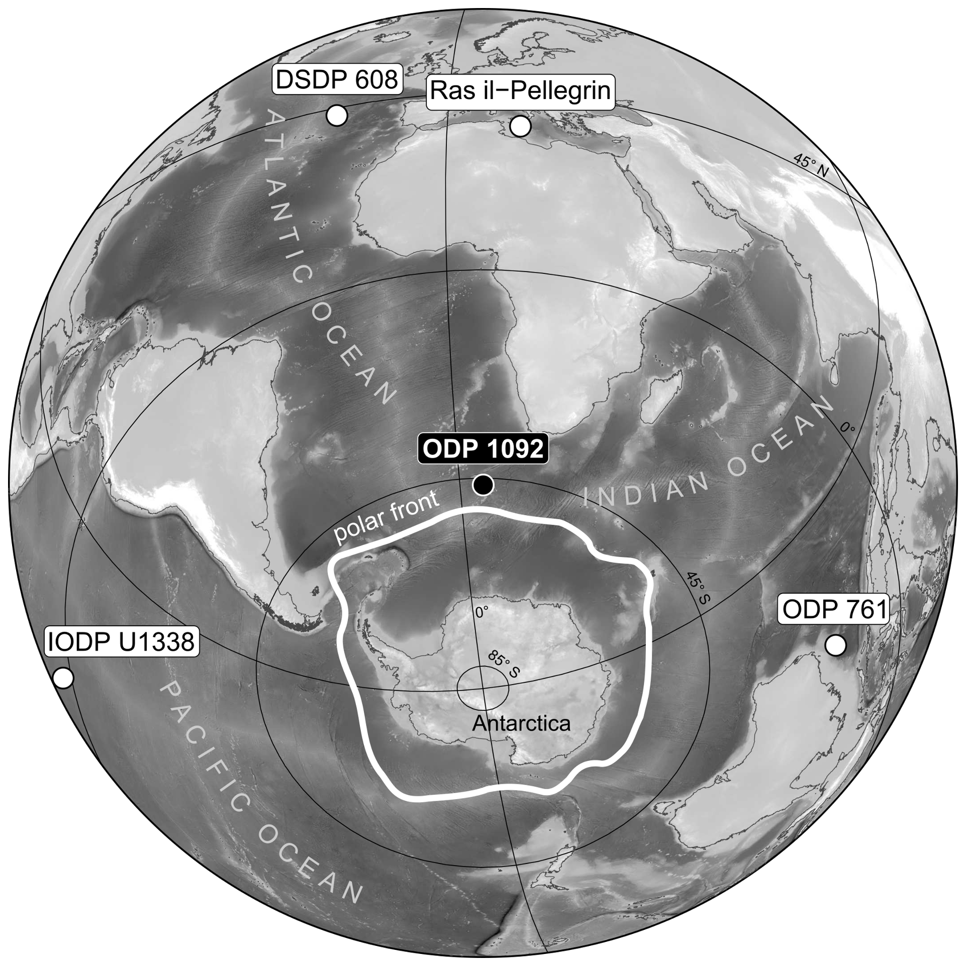
Figure 1 Azimuthal view of the location of ODP Site 1092 (water depth 1973 m) on the Meteor Rise in the South Atlantic Ocean, north of the modern polar front. Also shown are locations of DSDP Site 608, ODP Site 761, IODP Site U1338, and Ras-il-Pellegrin on Malta, for which pCO₂ records are displayed in Fig. 6.

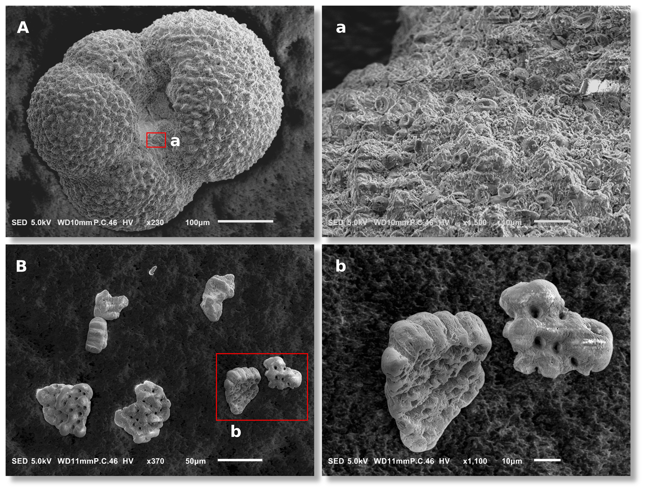
Figure 2 Scanning electron microscopy images of collected G. bulloides for δ¹¹B analysis (representative example from 177-1092B-18-4, 69–71 cm): (A) whole shell; (a) close-up image that reveals intact coccoliths covering the shell surface, indicating a lack of post-depositional dissolution; (B) shell fragments after chemical cleaning; and a (b) close-up image showing the absence of non-shell material.

2 Material and methods

2.1 Sampling strategy

This research used samples from Ocean Drilling Program (ODP) Site 1092, located at 46.41^∘ S and 7.08^∘ E (Fig. 1) at a water depth of 1973 m. The interval studied (∼ 178–184 mcd; see Table S1 in the Supplement) consists of nannofossil ooze with excellent carbonate preservation, as shown by undissolved coccoliths, which are susceptible to corrosion (Fig. 2). The shown example is from ∼ 13.8 Ma, where pH was low, but shell preservation is similarly good throughout the entire record. From the 250–315 µm size fraction, approximately 200 specimens (∼ 2.5 mg) of the cold-water-dwelling planktonic foraminifer G. bulloides were picked for δ¹¹B analysis from 35 processed 10 cm³ sediment samples. In addition, about five to eight specimens of the benthic foraminifer Cibicidoides wuellerstorfi were picked from 14 intervals to reconstruct deep-sea pH (Table S1). Today, surface-water pCO₂ at Site 1092 is close to equilibrium with the atmosphere (ΔpCO${}_{\text{2sea-air}}<-\mathrm{30}$ µatm; Takahashi et al., 1993, 2009). Plankton tow data revealed that G. bulloides in the Atlantic sector of the Southern Ocean is predominantly found within the upper 100 m of the water column (Mortyn and Charles, 2003). Based on DIC (dissolved inorganic carbon) and TA (total alkalinity) from seasonal TCO2+TALK (Goyet et al., 2000) and temperature and salinity from WOA13 data sets, modern gradients in pH and pCO₂ are small at this site within the upper 200 m of the water column. During the austral spring season, when the shell flux of G. bulloides is highest (Jonkers and Kučera, 2015; Raitzsch et al., 2018), the differences in pH and pCO₂ within this depth range are −0.03 and 17 µatm, respectively. Hence, we expect G. bulloides to be a reliable recorder of subsurface pH and pCO₂.

2.2 Age model

The age model used in this study is adopted from Kuhnert et al. (2009) but was revised to bring it in line with the astronomically tuned stable isotope record of the reference IODP Site U1338 (Holbourn et al., 2014) (Fig. 3, Table S2). For direct comparison of our pCO₂ record with the boron-based reconstructions available from the literature, the age models of ODP 761 (Holbourn et al., 2004; Foster et al., 2012; Sosdian et al., 2018) and the Blue Clay Formation of Ras-il-Pellegrin on Malta (Abels et al., 2005; Badger et al., 2013) were also retuned to match the reference curve U1338 (Table S2). Although the global stratotype section and point (GSSP) of the Langhian–Serravallian boundary (Mi-3b) in the Malta section was not explicitly placed at 13.82 Ma as suggested by Abels et al. (2005), the boundary in the revised age model (13.81 Ma) is in very close agreement, supporting the validity of the retuned record. Based on these revised age models, the δ¹⁸O and δ¹³C profiles of Sites 1092, ODP 791, and the Blue Clay Formation generally show a good agreement with those of Site U1338 (Fig. 3).

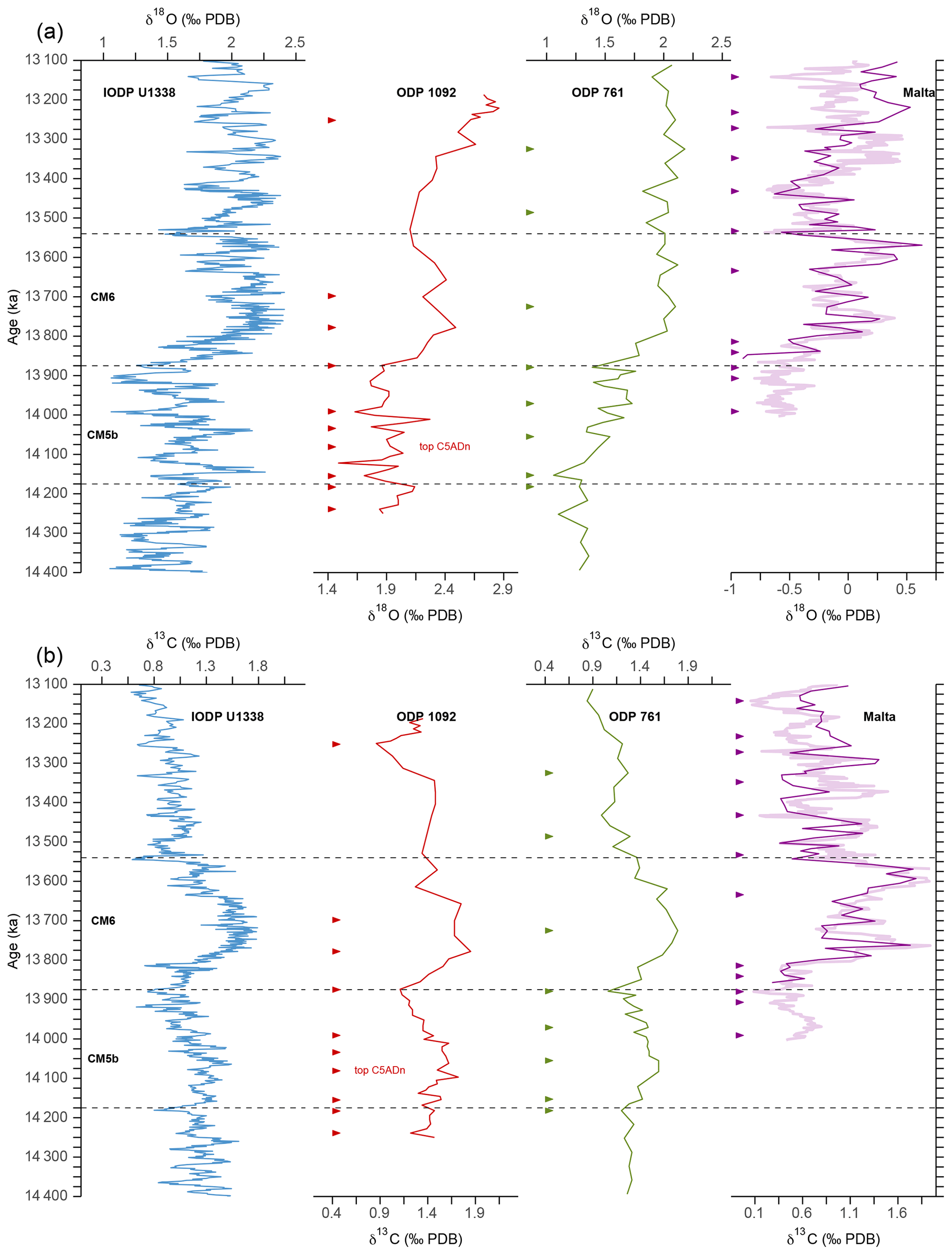
Figure 3 Age models of ODP Site 1092, ODP Site 761, and the Blue Clay Formation (Ras-il-Pellegrin, Malta), which were retuned with respect to the reference curve of IODP Site U1338 (Holbourn et al., 2014), based on their δ¹⁸O (a) and δ¹³C (b) records. The thick line in the Ras-il-Pellegrin record is from Abels et al. (2005), and the thin line is from Badger et al. (2013). Arrows mark tie points from this study, which are listed in Table S2. Dashed lines delimit CM events 5b and 6.

2.3 Boron isotope analysis

Foraminifer shells were cleaned following the protocol of Barker et al. (2003). Boron (B) isotope ratios were measured following Raitzsch et al. (2018). Briefly, the cleaned samples were dissolved in 60 µL of 1 N HNO₃ and micro-distilled on a hotplate to separate boron from the carbonate matrix. The micro-distillation method has been proven to yield a B recovery of ∼ 100 %, a low procedural blank, and accurate results, even at low B concentrations (Gaillardet et al., 2001; Wang et al., 2010; Misra et al., 2014; Raitzsch et al., 2018). The procedural blank contribution was 10–50 pg B, which equates to ∼ 0.2 %–0.8 % of the total [B] in the micro-distillation vial. The distillate containing only boron was diluted with 2 % HNO₃ and analyzed for isotopes in triplicate using a Nu Plasma II multi-collector inductively coupled plasma mass spectrometry (ICPMS) at AWI (Bremerhaven, Germany) that is equipped with a customized detector array of 16 Faraday cups and 6 secondary electron multipliers (SEM), also termed ion counters (IC). The ¹¹B and ¹⁰B samples were collected in IC5 and IC0, respectively, at a boron concentration of ∼ 3 ppb. As three of the SEMs were later replaced by Daly detectors, ¹¹B and ¹⁰B of C. wuellerstorfi samples were collected in D5 and D0, respectively, at a boron concentration of ∼ 2 ppb. ¹¹B/¹⁰B was standardized against concentration-matched NBS 951 using the standard–sample–standard bracketing technique, and frequent analysis of control standard AE121 with an isotopic composition similar to that of foraminifers was monitored to ensure accuracy of measurement. Measurement uncertainties are reported as 2 standard deviations (2σ) derived from triplicate measurements or as ±0.30 ‰ (for SEM-analyzed samples) and ±0.25 ‰ (for Daly-analyzed samples) determined from the long-term reproducibility (2σ of per-session δ¹¹B averages) of the control standard, whichever is larger (see Table S1).

2.4 Calculation of carbonate chemistry

To reconstruct pH and pCO₂ for the middle Miocene from the boron isotopic composition of foraminiferal shells, more constraints and assumptions of boundary conditions need to be made, as the ocean chemistry was different from today. This includes the boron isotopic composition of seawater (δ¹¹B_sw), which has a direct effect on that of foraminifer shells (δ¹¹B_foram) but also on the δ¹¹B${}_{\mathrm{foram}}/{\mathit{\delta }}^{\mathrm{11}}$B_borate relationship, which in turn may lead to different pH yields. Further, we need to consider the seawater concentrations of calcium [Ca] and magnesium ions [Mg], which affect both the ocean's buffering capacity and the Mg $/$ Ca ratios in foraminifer shells used to reconstruct seawater temperatures. Ultimately, we need to constrain a second carbonate system parameter (besides pH) to determine absolute atmospheric pCO₂ values as accurately as possible.

2.4.1 δ¹¹B of seawater

The most critical parameter for correct conversion of δ¹¹B_foram to pH is δ¹¹B_sw, which is fortunately well constrained for the middle Miocene. We used a δ¹¹B_sw value of 37.80 ‰, which is the mean value from different independent studies and in close agreement with each other to within 0.2 ‰ (2σ) (Pearson and Palmer, 2000; Foster et al., 2012; Raitzsch and Hönisch, 2013; Greenop et al., 2017), and also comparable to the 38.5 ‰ modeled by Lemarchand et al. (2000). This value is used for both the calculation of pH and the adjustment of the δ¹¹B${}_{\mathrm{foram}}/{\mathit{\delta }}^{\mathrm{11}}$B_borate regression intercept, where the effect is larger the more the slope differs from a 1 : 1 relationship (Greenop et al., 2019). Nonetheless, to inspect the influence of δ¹¹B_sw on final reconstructed pCO₂ values, we carried out the calculations using lower and upper extremes in δ¹¹B_sw of 36.80 ‰ and 38.80 ‰, respectively. The results show that the extreme scenarios not only reveal differences in reconstructed pCO₂ of up to 320 µatm but also in relative changes, due to the nonlinearity of the δ¹¹B-pH proxy (Fig. S1). However, we propose that a δ¹¹B_sw value of 37.80 ‰ is a reasonable estimate, given the close agreement between independent studies and the closeness to non-boron-based pCO₂ reconstructions.

2.4.2 Equilibrium constants

As the Miocene ocean had different [Ca] and [Mg] than today, their separate effects on seawater buffering must be taken into account to more accurately estimate past carbonate chemistry. For our study, all carbonate system parameters were calculated based on the MyAMI model (Hain et al., 2015; 2018) using a [Ca] and [Mg] of 13 and 42 mmol kg⁻¹, respectively, derived from halite fluid inclusions (Horita et al., 2002; Lowenstein et al., 2003; Timofeeff et al., 2006; Brennan et al., 2013).

2.4.3 Foraminiferal δ¹¹B calibrations

The different species-specific δ¹¹B${}_{\mathrm{foram}}/{\mathit{\delta }}^{\mathrm{11}}$B_borate calibrations used to reconstruct Miocene pH may ultimately result in significantly different pCO₂ estimates (Fig. S2). For G. bulloides, there are three calibrations available (Martínez-Botí et al., 2015; Henehan et al., 2016; Raitzsch et al., 2018), all of which yield very similar results (Fig. S2a). In this study, we used the one from Raitzsch et al. (2018) giving values that lie between the other two estimates. By contrast, for Trilobatus trilobus δ¹¹B the Trilobatus sacculifer calibration is applied, with four available equations (Foster et al., 2012; Martínez-Botí et al., 2015; Henehan et al., 2016; Dyez et al., 2018). The calibrations refer to different size fractions of T. sacculifer and different analytical techniques, resulting in Miocene pCO₂ estimates that differ from each other by up to ∼ 2000 µatm (Fig. S2b, c). The very high pCO₂ (low pH) values obtained with the equation from Dyez et al. (2018) are attributed to the much shallower slope (data collected with negative thermal ionization mass spectrometry; N-TIMS), compared to those of the other calibrations (based on MC-ICPMS measurements). Due to the lower δ¹¹B_sw in the Miocene, this lower sensitivity also requires a stronger adjustment of the regression towards a higher intercept (Greenop et al., 2019), which results in calculations of even lower pH values. Hence, we assume that the calibration of Dyez et al. (2018) is not suitable for deep-time studies, when the δ¹¹B_sw was much different from today, using MC-ICPMS. However, the calibrations of Martínez-Botí et al. (2015) and Henehan et al. (2016) also result in Miocene pCO₂ estimates up to 400 µatm higher than the G. bulloides data (Fig. S2a) and other, non-boron-based, pCO₂ proxy data. Therefore, we retained the original equation provided by Foster et al. (2012) to re-evaluate the δ¹¹B data of their study and the study by Badger et al. (2013).

2.4.4 pH and temperature estimates

δ¹¹B_foram was converted to δ¹¹B_borate using the calibration for G. bulloides from Raitzsch et al. (2018), which was adjusted for the lower δ¹¹B_sw following Greenop et al. (2019). Subsequently, pH was calculated using sea-surface temperatures (SSTs) derived from foraminiferal Mg $/$ Ca ratios, a hydrostatic pressure of 5000 hPa (equivalent to 50 m water depth), and salinity based on the study by Kuhnert et al. (2009). The latter was estimated by converting δ¹⁸O_sw, derived from planktonic foraminiferal δ¹⁸O and Mg $/$ Ca temperatures (Shackleton, 1974), to salinity using a δ¹⁸O_sw : salinity gradient of 1.1 ‰ (the change in δ¹⁸O_sw per salinity unit). This minimum gradient is required to keep the upper-ocean density difference across the Subantarctic Front to enable the formation of Antarctic Intermediate Water (Kuhnert et al., 2009), which existed as Southern Component Intermediate Water (SCIW) since at least ∼ 16 Ma (Shevenell and Kennett, 2004) and spread into all oceans adjacent to the Southern Ocean (Wright et al., 1992). The relative salinity record was then adjusted by 17.2 to achieve post-glaciation values similar to today. The reconstructed relative salinity change across the MMCT at Site 1092 is slightly more than 1, which is equivalent to the salinity gradient across the Subantarctic Front today.

As seawater pH has a profound effect on foraminifer shell Mg $/$ Ca, biasing reconstructed SSTs, which in turn results in altered pH estimates, we followed the method of Gray and Evans (2019) to iteratively solve Mg $/$ Ca temperatures and δ¹¹B-derived pH. For this, we modified the “MgCaRB” R script of Gray and Evans (2019) to allow salinity and δ¹¹B_sw as additional input parameters (see code in Sect. S1 in the Supplement). In addition, we implemented a correction of shell Mg $/$ Ca for changes in seawater Mg $/$ Ca ([Mg $/$ Ca]_sw) using the method of Evans and Müller (2012), where we applied the power function constants for Trilobatus sacculifer, assuming that they are valid for other low-Mg foraminifers as well. In this study, we used a Mg $/$ Ca_sw that was likely on the order of 3.2 mol mol⁻¹ at ∼ 14 Ma, inferred from the chemical composition of halite fluid inclusions (Horita et al., 2002; Lowenstein et al., 2003; Timofeeff et al., 2006; Brennan et al., 2013).

To better compare our record with published boron-based pCO₂ reconstructions, the δ¹¹B and Mg $/$ Ca data of T. trilobus from Foster et al. (2012) and Badger et al. (2013) were re-evaluated using the same calculation procedure as for our data. Here, we used the calibration for T. sacculifer from MgCaRB, although there is no discernable pH effect on the Mg $/$ Ca of this species. Further, we applied a constant salinity of 35 and a hydrostatic pressure of 0 Pa, but their effects on the final results are almost negligible as well.

Deep-sea temperatures were derived from Mg $/$ Ca of C. wuellerstorfi (data courtesy of Henning Kuhnert) using the species-specific calibration of Raitzsch et al. (2008), but we multiplied the pre-exponential constant with 0.825 (Evans and Müller, 2012) to correct temperatures for the lower Mg $/$ Ca_sw of the Miocene (see caption Table S1). Deep-ocean pH from the same species was calculated using a δ¹¹B${}_{\mathrm{foram}}/{\mathit{\delta }}^{\mathrm{11}}$B_borate calibration (Table S1) fitted through core-top data from Rae et al. (2011) and Raitzsch et al. (2020), a salinity of 34, and a paleo-water depth of 1794 m.

The uncertainties for all pH and temperature values reported here were propagated using Monte Carlo simulations (10 000 repetitions) and comprise quoted 2σ uncertainties for δ¹¹B and Mg $/$ Ca measurements, δ¹¹B${}_{\mathrm{foram}}/{\mathit{\delta }}^{\mathrm{11}}$B_borate calibrations, δ¹¹B_sw (±0.2 ‰), salinity (±1), and the reciprocally corrected pH and temperatures calculated by MgCaRB (Gray and Evans, 2019).

2.4.5 pCO₂ reconstruction

To calculate pCO₂ from sea-surface pH, a second carbonate system parameter needs to be constrained. For this study, we used a sea-surface TA of 2000 µmol kg⁻¹, which is in line with various carbon cycle model results (Tyrrell and Zeebe, 2004; Ridgwell, 2005; Caves et al., 2016; Sosdian et al., 2018; Zeebe and Tyrrell, 2019), and we applied it to the entire record. However, to verify the validity of our approach we tested the effect of varying TA on pCO₂ calculations (see Sect. 3.3). Uncertainties of pCO₂ estimates were fully propagated from adjusted 2σ uncertainties in pH and temperature (produced by MgCaRB; see Sect. 2.4.4), TA (±150 µmol kg⁻¹), and salinity (±1 psu) using the “seacarb” package (Lavigne et al., 2011) programmed in “R”. The applied temperature uncertainty is similar to the mean difference of ∼ 2 ^∘C between the non-corrected and pH-corrected Mg $/$ Ca temperatures (Fig. S3), while the TA uncertainty encompasses the mean standard deviation of $\pm \sim$ 130 µmol kg⁻¹ between different TA models and the standard deviation of $\pm \sim$ 50 µmol kg⁻¹ for each model across the MMCT (Sosdian et al., 2018). The applied salinity uncertainty encompasses the potential salinity change across the MMCT.

3 Results

3.1 Carbon dioxide record

Our boron-based record indicates a steady pCO₂ increase from ∼ 380 to 520 ± 100 µatm between 14.25 and 14.08 Ma and a subsequent decrease to ∼ 320 µatm until 13.87 Ma, culminating after the onset of the major ice-sheet expansion (Fig. 4e). It should be noted that this ∼ 200 µatm drop in pCO₂ occurred at a time of northward-shifting Southern Ocean fronts, which is only related to a step-like drop in SST and salinity around 14 Ma at this site (Fig. 4c) (Kuhnert et al., 2009). At 13.82 Ma, when SST had already reached a lower stable level and after the inception of the ∼ 1 ‰ rise in benthic δ¹⁸O (Fig. 4a), pCO₂ increased rapidly by ∼ 100 µatm and displayed high-amplitude variations of more than 50 µatm until 13.57 Ma. This transient rise in pCO₂ ended with a decrease to ∼ 320 µatm and much reduced variability after 13.53 Ma (Fig. 4e). Despite the high 2σ uncertainty of ∼ 100 µatm for the overall pCO₂ record, the interpretation of comparatively small changes of ∼ 50 µatm is reasonable, due to the smaller uncertainty of relative variations. The latter is estimated to be approximately 50 µatm (2σ), i.e., when uncertainties in the δ¹¹B${}_{\mathrm{foram}}/{\mathit{\delta }}^{\mathrm{11}}$B_borate calibration and δ¹¹B_sw are neglected. Sea-surface pH values within the entire record range from 7.94 to 8.11 ± 0.09, while deep-sea pH varies between 7.77 and 7.87 ± 0.08 over the same interval (Figs. 4d and S4). Interestingly, the pH offset between the surface and deep ocean is nearly identical to the modern gradient and apparently does not change substantially within our Miocene record (Fig. S4), but the high uncertainties associated with the pH estimates hamper a reasonable statistical analysis of the temporal change in gradient.

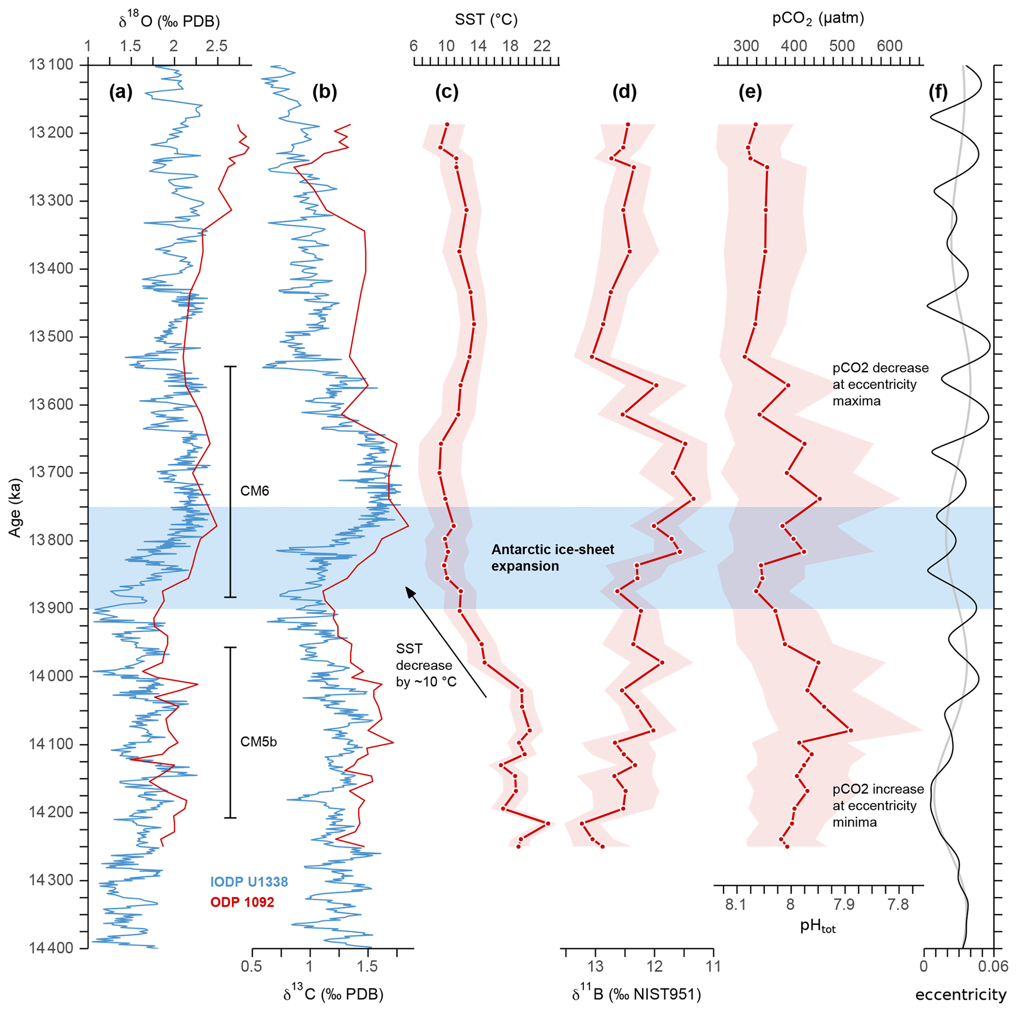
Figure 4 Proxy records of the middle Miocene climate transition. (a) Benthic oxygen isotope curve from ODP Site 1092 (in red) used in this study and from eastern Pacific IODP Site U1338 (in blue) used as a reference (Holbourn et al., 2014). (b) The same as in panel (a) but for carbon isotopes. The carbon maximum events CM5b and CM6 are indicated. (c) Site 1092 sea-surface temperatures based on G. bulloides Mg $/$ Ca ratios (Kuhnert et al., 2009) and pH-adjusted following Gray and Evans (2019) with a 2σ uncertainty band. (d) Raw boron isotope data of G. bulloides. Shaded area indicates 2σ uncertainties of measurement. (e) Estimated pCO₂ of surface waters basically using temperature-adjusted δ¹¹B-based pH following Gray and Evans (2019), a total alkalinity (TA) of 2000 ± 150 µmol kg⁻¹, and a δ¹¹B_sw value of 37.80 ± 0.2 ‰. Note that the secondary axis only approximates corresponding pH and that the shaded area delimits propagated uncertainties only for pCO₂. For exact pH values and uncertainties, see Fig. S4. (f) Eccentricity of the Earth's orbit is from Laskar et al. (2004) and a low-pass-filtered 400 kyr signal (grey line).

The pCO₂ variations within the studied time interval show a remarkable agreement with variations in δ¹³C that correspond to CM5b and CM6 (Fig. 4). Accordingly, the maxima at ∼ 14.1 and 13.7 Ma as well as the minima at ∼ 13.9 and 13.5 Ma, indicate that atmospheric CO₂ levels were paced by 400 kyr cycles, as also demonstrated by evolutive harmonic and power spectral analyses (Fig. 5), but due to the phase lag it is difficult to substantiate a direct link between long eccentricity cycles and atmospheric CO₂.

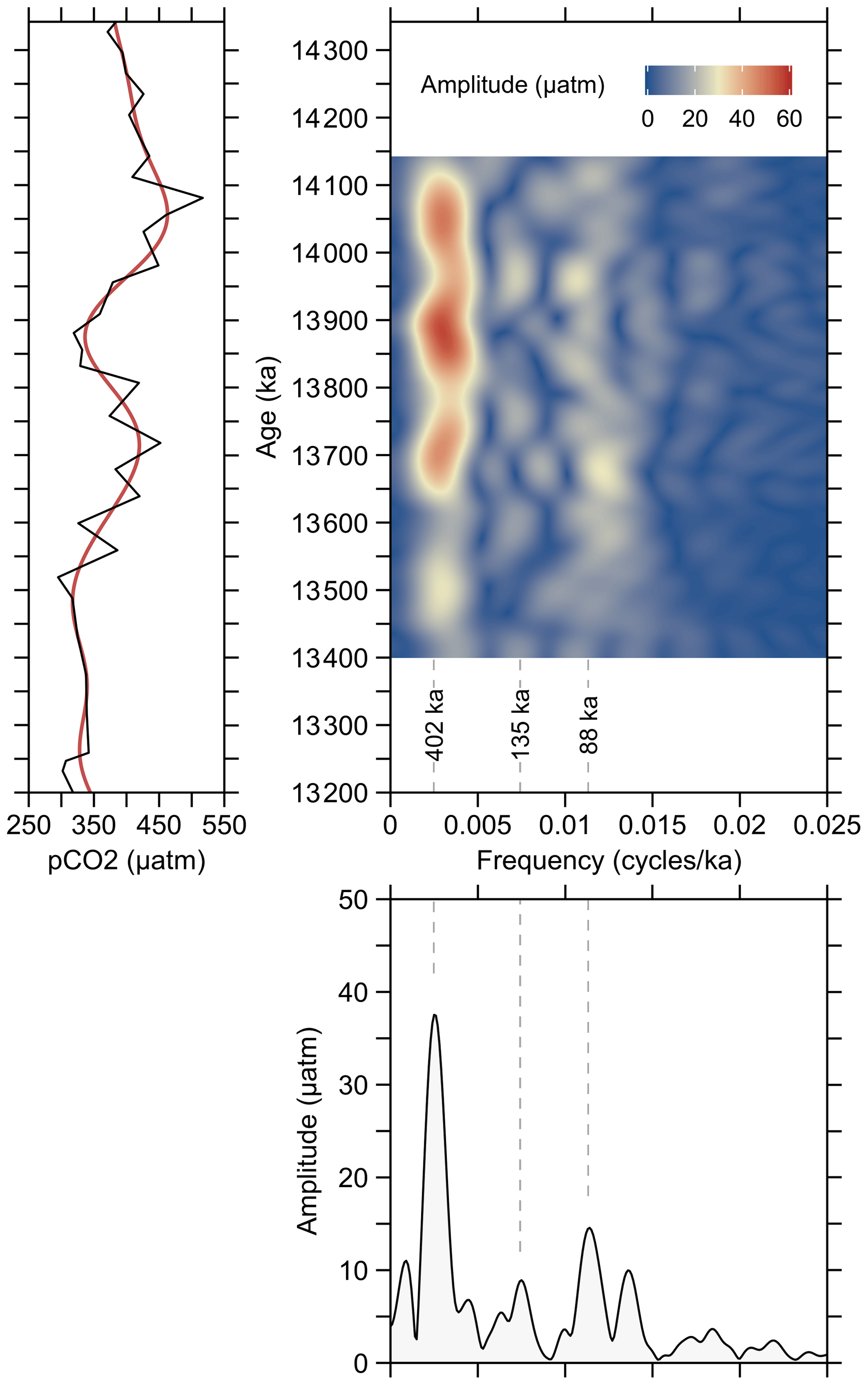
Figure 5 Evolutive harmonic analysis (EHA) and power spectral analysis of pCO₂ record from ODP Site 1092, using the Thomson multitaper method (MTM). The red line in the left panel is the low-pass-filtered 400 kyr signal using cosine-tapered window. Analyses were performed using the R package “Astrochron” (Myers, 2014).

3.2 Sea-surface temperatures

Due to the profound effect of pH on Mg $/$ Ca in shells of G. bulloides, which might bias reconstructed SSTs, we applied the modified MgCaRB tool of Gray and Evans (2019) to iteratively solve Mg $/$ Ca temperatures and δ¹¹B-derived pH. In addition, we applied a correction factor to account for the effect of [Mg $/$ Ca]_sw on shell Mg $/$ Ca using the method of Evans and Müller (2012). However, to evaluate the difference between iteratively adjusted and non-adjusted pH and temperature values, we also performed the conventional calculations using the G. bulloides δ¹¹B calibration from Raitzsch et al. (2018) and Mg $/$ Ca-to-temperature component from Gray and Evans (2019), respectively. It should be noted that the Mg $/$ Ca sensitivity of G. bulloides to temperature determined by Gray and Evans (2019) is much larger than that by Mashiotta et al. (1999). Therefore, the calculated unadjusted temperature decrease between 14.05 and 13.85 Ma is on the order of 13 ^∘C, compared to ∼ 6 ^∘C determined with the equation of Mashiotta et al. (1999) and reported in Kuhnert et al. (2009). After the iterative correction of Mg $/$ Ca and pH, the results show that before the EAIS expansion the adjusted temperature and pCO₂ values are up to ∼ 3 ^∘C and ∼ 60 µatm lower, respectively (Fig. S3). On the contrary, after 13.9 Ma the adjusted temperature and pCO₂ reconstructions are very similar, suggesting that approximately one-fourth of the observed pre-glacial Mg $/$ Ca decrease was induced by a contemporaneous pH rise.

3.3 Sensitivity tests

Given that we use TA as the second variable to calculate the inorganic carbon chemistry, which might affect calculated pCO₂ discernibly, we carried out a number of sensitivity tests. The first tests demonstrate that either constant salinity, a ∼ 1 unit change in salinity, or TA co-varying with salinity using a modern TA–S relationship (∼ 42 µ mol kg⁻¹ per S unit), has no discernible effect on pCO₂ estimates (Fig. S5a). As ODP Site 1092 was apparently influenced by a northward migration of the Southern Ocean fronts, we tested the potential impact on calculated pCO₂ by coupling TA to temperature. Even at an unrealistically high total change of 400 µmol kg⁻¹, calculated relative pCO₂ changes are similar after the EAIS expansion at ∼ 13.9 Ma (Fig. S5b). Given the modern sea-surface TA gradient across the polar frontal system of ∼ 100 µmol kg⁻¹ (higher in the south), we conclude that the increasing influence of southern-sourced surface waters on pCO₂ estimates at our study site is comparatively small. When in our simulations TA was coupled to pH (Fig. S5c, d) or eccentricity (Fig. S5e–h) by ±100 µmol kg⁻¹, pCO₂ reconstructions are almost identical among each other. On the other hand, at TA variations of ±400 µmol kg⁻¹, the pCO₂ estimates may differ substantially between the different scenarios, but the general shape of the record remains more or less the same. Given that total variations in TA of 800 µmol kg⁻¹ are very unlikely, we suggest that potential variations in TA do not affect our pCO₂ estimates significantly.

4 Discussion

4.1 Origin of Site 1092 pCO₂ signal

At face value, the reconstructed pCO₂ curve displays a remarkable resemblance to the global benthic δ¹³C record (Fig. 4), suggesting that there is a first-order link between the two. Our record, however, is the first that shows an increase of pCO₂ after the onset of Antarctic glaciation, which is counterintuitive at first glance, given that most hypotheses refer to enhanced C_org burial as the main mechanism having caused the rise in δ¹³C and presumably an atmospheric CO₂ drawdown. Hence, this raises the question as to whether Site 1092 truly records a global pCO₂ signal or a local one instead. It is difficult to tackle this question because we neither have a complete, independent pCO₂ reconstruction for this time interval at similar or higher resolution for comparison, nor can we ascertain that any site millions of years ago was not influenced by local processes affecting the geochemical signal. Therefore, we cannot completely rule out a local or regional imprint on our pCO₂ record, particularly due to the proximity of Site 1092 to the polar front (Fig. 1).

There is indication for development of the subantarctic ocean frontal system and a better stratification of the upper ocean at Site 1092 following Antarctic ice-sheet expansion, suggested by a divergence in δ¹⁸O between shallow- and deep-dwelling planktonic foraminifera (Paulsen, 2005). Although the occurrence of ocean fronts should have involved changes in biological productivity that may result in altered surface-water [CO₂], the opal and C_org contents in the sediment remain steadily low throughout the middle Miocene (Diekmann et al., 2003), suggesting that Site 1092 was in an oligotrophic setting within the time interval studied. Moreover, if the δ¹¹B signal was mainly driven by a regional change in stratification after 13.85 Ma, this would not explain the low pH earlier during CM5, as shown in our record (Fig. 4).

Further, a better stratification should have resulted in a reduced vertical mixing of the water column and thus to reduced sea–air gas exchange, leading to decreased atmospheric CO₂, such as in the Southern Ocean during the Last Glacial Maximum (François et al., 1997). On the contrary, our data do not imply such a situation, as the pH gradient between deep and surface ocean appears to have remained constant (Fig. S4), suggesting that DIC accumulated in both shallow and deep waters at this site, which resulted in an overall pH decrease. Indeed, Leutert et al. (2020) suggested that the expansion of the Antarctic Circumpolar Current (ACC) following ice-sheet expansion could have moved the frontal systems and westerly winds further north, which reduced Southern Ocean upwelling and hence provided a mechanism to increase carbon storage in the deep ocean, drawing down pCO₂. If the deep ocean in the south was indeed less well ventilated, we would expect benthic δ¹³C to decrease after the onset of the EAIS expansion because the ocean had more time to accumulate ¹³C-depleted CO₂ from decomposed C_org, which is the opposite (increasing δ¹³C, Fig. 4). All these complications call for more proxy records at sufficient resolution from spatially distinct locations to better constrain pCO₂ evolution across the MMCT.

4.2 Comparison with other pCO₂ records

Our pCO₂ data broadly agree with reconstructed long-term trends based on paleosol δ¹³C (Ji et al., 2018) and planktonic foraminiferal δ¹¹B (Foster et al., 2012), except for the higher value at ∼ 14.2 Ma (Fig. 6). The boron isotope data from the Mediterranean Sea by Badger et al. (2013) also show pCO₂ values that match our data well after 13.8 Ma, but our data do not exhibit a generally higher pCO₂ level immediately before 13.8 Ma. On the one hand, the relative pH increase of ∼ 0.1 accompanying Antarctic glaciation was backed up by comparing a pH-dependent (Mg $/$ Ca) with independent temperature proxies (clumped isotopes and TEX₈₆) obtained from the same set of samples (Leutert et al., 2020). On the other hand, the strong SST decrease of ∼ 4–5 ^∘C after the onset of Antarctic glaciation, as suggested by the Mediterranean data, is more than 2 ^∘C larger than those recorded in other low-latitude sites (Foster et al., 2012; Leutert et al., 2020; Sosdian and Lear, 2020), yet the reason for this discrepancy needs to be examined. In contrast, the pCO₂ reconstruction based on alkenone δ¹³C data from Badger et al. (2013) is similar to the estimates of Super et al. (2018), which are generally lower than the boron-based data and do not exhibit significant changes during CM6. Recent studies suggest that phytoplankton may enhance cellular carbon supply for photosynthesis via carbon concentrating mechanisms under limited aqueous [CO₂], making this proxy less sensitive at low to moderate pCO₂ levels (Badger et al., 2019; Stoll et al., 2019).

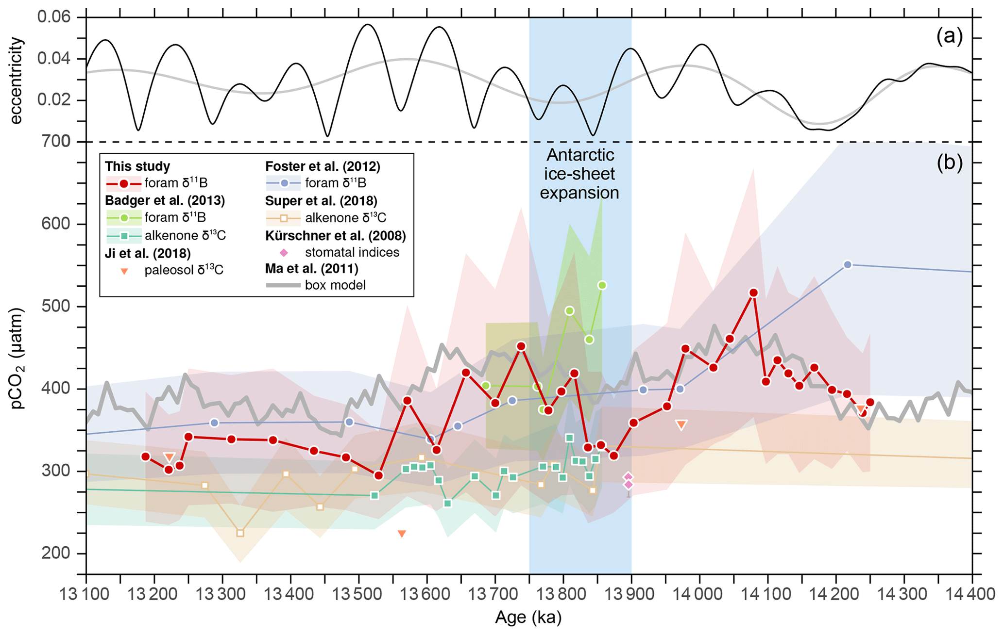
Figure 6 Eccentricity of the Earth's orbit from Laskar et al. (2004) (a) and a comparison of pCO₂ estimates from this study with literature data (b). Note that for pCO₂ reconstructions from Foster et al. (2012) and Badger et al. (2013), the boron-based pH data were recalculated using the MgCaRB tool (Gray and Evans, 2019) modified for deep-time reconstructions (code in Sect. S1), a TA of 2000 ± 150 µmol kg⁻¹, and a δ¹¹B_sw value of 37.80 ± 0.2 ‰ for consistency with our data. In addition, the age models from these studies were also revised for direct comparison with our record (Fig. 3). All other records are based on their original data and age models.

There is no other direct evidence for increasing pH immediately following the onset of EAIS expansion than the δ¹¹B data by Badger et al. (2013), which is supported by Sosdian et al. (2020) who used planktonic foraminiferal B $/$ Ca ratios from ODP Site 761 (Fig. 1) to infer relative changes in DIC across the middle Miocene. As B $/$ Ca in planktonic foraminifera is thought to be governed by the ratio between borate and DIC concentrations [B(OH${)}_{\mathrm{4}}^{-}$ $/$ DIC], an increase in B $/$ Ca can be interpreted as a decrease in DIC and/or an increase in [B(OH${)}_{\mathrm{4}}^{-}$] (e.g., Allen et al., 2012). The high-resolution B $/$ Ca record of Sosdian et al. (2020) reveals that the long-lasting Monterey excursion is accompanied by generally low B $/$ Ca ratios, whereas CM intervals are characterized by higher B $/$ Ca, suggesting periodic DIC decreases within a “high-DIC” world. The authors concluded that during the CM events, ice-sheet expansion and global cooling enhanced marine productivity and C_org burial, which resulted in a reduction of surface-water DIC and pCO₂, and a rise in δ¹³C.

Within the overlapping period, which encompasses two full 400 kyr cycles, our record exhibits some striking similarities with the B $/$ Ca record of Sosdian et al. (2020), including the long-term decrease in pCO₂, accompanied by declining surface-water DIC, and the higher pCO₂ during CM5b (Fig. 6) that is accompanied by increased DIC. Intriguingly, the correlation between the two records collapses at the onset of CM6, when the B $/$ Ca record indicates a decline in DIC, which is corroborated by a lowering in pCO₂ (Badger et al., 2013). This is in contrast to our record showing that pCO₂ increased during CM6 (Fig. 4), although the records are once again in agreement at the end of CM6 (∼ 13.5 Ma). This discrepancy could be attributed to non-identified factors influencing either of the two proxies or regional effects on either of the two records. The potential influence of the polar front on Site 1092 is addressed in Sect. 4.1, leading to the question of whether the data by Sosdian et al. (2020) could be alternatively explained by increased deep-water production. When the density of surface waters in the Southern Ocean increased due to cooling in a generally warm middle Miocene, the invigorated deep-ocean venting could have brought respired CO₂ to the atmosphere, leaving the overall ocean depleted in DIC and enriched in CO${}_{\mathrm{3}}^{\mathrm{2}-}$ and possibly also in δ¹³C. The higher CO${}_{\mathrm{3}}^{\mathrm{2}-}$ in turn could have favored the burial of carbonate in the deep sea, producing even more CO₂ that is vented to the atmosphere, as suggested for the Pleistocene glacial–interglacial cycles (Toggweiler, 2008). This way, the loss of CO₂ in shallow waters, caused by enhanced marine productivity and C_org burial (Sosdian et al., 2020), could have been outweighed by CO₂ added to the atmosphere by deep-ocean ventilation. However, this is speculative and needs to be validated in future studies.

It is worth noting that our pCO₂ record before Antarctic glaciation reveals a striking match with the box model output from Ma et al. (2011), while after EAIS expansion our values are some 50 µatm lower, although they still exhibit similar relative changes (Fig. 6). The divergence after ∼ 13.9 Ma may be related to the model by Ma et al. (2011), which was designed to simulate orbitally paced carbon reservoir changes for the Miocene Climate Optimum (MCO) and hence does not include ice sheets. Consequently, the model does not consider the effects of falling sea level on the shelf-to-basin fractionation of carbonate burial (McKay et al., 2016; Ma et al., 2018), or of ice-sheet expansion on ocean circulation and bottom-water ventilation (e.g., Shevenell et al., 2004; Holbourn et al., 2007, 2013), all of which should have influenced δ¹³C and pCO₂. However, the similarity between our record and the model suggests that the ocean carbon reservoir varied in response to weathering-induced nutrient input, which in turn was controlled by varying orbital configuration. This model was sufficient to explain the observed δ¹³C pattern of the MCO (Ma et al., 2011) but could also be capable of explaining a portion of the observed carbon cycle changes in a world with an ice-covered Antarctica.

4.3 The role of weathering in the carbon cycle

The pCO₂ increase preceding and following the EAIS expansion closely tracks the global δ¹³C history of CM5b and CM6 (Fig. 4), emphasizing a fundamental link between changes in the ocean carbon cycle and atmospheric carbon dioxide. The CM peaks correspond to minima in the 400 kyr eccentricity cycle, suggesting that δ¹³C variations were related to changes in monsoon and weathering intensity (Holbourn et al., 2007; Ma et al., 2011). Eccentricity maxima lead δ¹³C minima at the 400 kyr band by on average more than 50 kyr, which is comparable to the phase lag of 47 ± 18 kyr observed in other Miocene records, which can possibly be attributed to the slow response of weathering to orbital forcing (Holbourn et al., 2007). Monsoon intensity is paced by solar radiation variations caused by precessional cycles but their amplitude variations are modified by eccentricity. More precisely, higher eccentricity results in larger precession amplitudes and hence in larger wet–dry variations in the tropics (e.g., Wang, 2009), stronger physical and chemical weathering, and ultimately in an increased input of particulate organic material, dissolved inorganic carbon, alkalinity and nutrients to the oceans (e.g., Clift and Plumb, 2008; Ma et al., 2011; Wan et al., 2009). The potential influence of alkalinity variations on our pCO₂ record is shown in Fig. S5 and evaluated in Sect. 3.3.

The increased nutrient supply enhanced primary production and organic carbon burial, which in turn lowered pCO₂. At the same time, the burial of shallow and total calcium carbonate (CaCO₃) increased, while CaCO₃ burial in the deep ocean decreased (Holbourn et al., 2007). However, as the net burial of CaCO₃ (enriched in ¹³C) in relation to C_org (depleted in ¹³C) increased at high eccentricity, δ¹³C_DIC values decreased, which is in line with the global isotope signature (Holbourn et al., 2007; Ma et al., 2011). Estimates of Miocene shallow-water carbonate burial and shelf–basin fractionation of carbonate accumulation are only available in rather low temporal resolution and do not capture orbital variability that would allow assessment of global trends (Boudreau and Luo, 2017; Boudreau et al., 2019; van der Ploeg et al., 2019). Another limitation is that attempts to estimate shallow water carbonate burial on an orbital timescale are limited to regional studies in very different environments (Kroon et al., 2000; Reuning et al., 2002; Williams et al., 2002; Aziz et al., 2003; Auer et al., 2015; Betzler et al., 2018; Ohneiser and Wilson, 2018; Reolid et al., 2019) that cannot be easily synthesized to provide global estimates.

An increase in carbonate burial in shallow seas would have removed alkalinity from seawater and thus lowered pH and released CO₂ to the atmosphere (e.g., Zeebe and Wolf-Gladrow, 2001) during 100 kyr eccentricity maxima; however, the resolution of our record is too low to detect this. On longer timescales (400 kyr cycles), increased alkalinity input from rivers, dissolution of deep-sea carbonates, and the enhanced burial of C_org in tropical regions during eccentricity maxima might have contributed to the long-term decrease in pCO₂. This agrees well with the box model output from Ma et al. (2011), suggesting that during the long-eccentricity maxima pCO₂ decreased, when the monsoon was most intense and the organic carbon burial and river fluxes were high. Conversely, weathering and nutrient supply to the ocean in low latitudes decreased when eccentricity was low, resulting in a net decrease in the CaCO₃-to-C_org burial ratio and hence in CO₂ release and higher δ¹³C.

The model of Ma et al. (2011) was designed to explain the long eccentricity signal in the δ¹³C record throughout the warm MCO and hence does not consider processes caused by expanding Antarctic ice sheets and their impacts on the climate system. Indeed, the modeled pCO₂ reveals smaller amplitudes after ∼ 13.9 Ma than our reconstruction (Fig. 6) and a less pronounced CM6 in relation to the previous CM events. Changes in shelf–basin partitioning of carbonate burial and enhanced global deep-water ventilation, as well as increased weathering, resulting from a major sea level fall at 13.8 Ma (Ma et al., 2018) are possible mechanisms to explain the higher amplitude of CM6. Additional mechanisms may have contributed to the amplification of CM6, including (1) increased C_org burial by enhanced carbon sequestration through the biological pump linked to intensified upwelling in low latitude areas, as well as (2) substantial outgassing of CO₂ from the deep ocean (δ¹³C of approx. −1 ‰ to −2 ‰) into the atmosphere (δ¹³C of approx. −6 ‰ to −6.5 ‰), which would not only result in increased atmospheric pCO₂ but also in a positive excursion in atmospheric δ¹³C. The size of the relevant reservoirs (38 000 Gt in the deep ocean vs. 750 Gt in the atmosphere, if the proportions were similar to today) would suggest that this process can be sustained over considerable time intervals. (3) The amplitude of the 405 kyr cycle-paced δ¹³C excursions depends on the size of the global marine DIC pool (e.g., Paillard and Donnadieu, 2014). This size may have decreased following the loss of shelf seas caused by the major regression associated with the onset of CM6, resulting in a higher amplitude δ¹³C response to eccentricity forcing.

4.4 Enhanced glacial deep-water ventilation

As stated in the previous section, the δ¹³C of CM6 might be related to global deep-water ventilation, due to cooling in the Southern Ocean that invigorated deep-water formation. The MMCT bears similarities to the Eocene–Oligocene transition (EOT) ∼ 34 Ma ago, when Antarctic ice expansion was also accompanied by a large positive δ¹³C excursion, in terms of both magnitude and duration (Coxall et al., 2005). The δ¹³C excursion following Antarctic glaciation was accompanied by a transient pCO₂ rise of more than 300 µatm (Pearson et al., 2009; Heureux and Rickaby, 2015), which bears similarity to the pCO₂ rise during the mid-Miocene EAIS expansion, although the amplitude was much larger. A modeling study suggested that a sea-level-fall-induced shelf-basin carbonate burial fractionation and a temporal enhancement of deep-water formation (by 150 %) in the Southern Ocean were sufficient to produce both the positive δ¹³C excursion and a transient pCO₂ rise by ∼ 80 µatm in the EOT (McKay et al., 2016).

Similarly, ocean circulation may have intensified during the Miocene EAIS expansion, as the latitudinal temperature gradient increased and atmospheric circulation strengthened. This is supported by benthic foraminifers, Mn $/$ Ca and XRF data from Southeast Pacific sites, which indicate improved deep-water ventilation and carbonate preservation after 13.9 Ma, particularly during colder climate phases (Holbourn et al., 2013). Improved deep-water ventilation may also have led to enhanced advection of silica-rich waters toward low latitudes, culminating in an increased upwelling and diatom productivity between 14.04 and 13.96 Ma and between 13.84 and 13.76 Ma in the equatorial East Pacific, as indicated by massive opal accumulation found at IODP Site U1338 (Holbourn et al., 2014). We speculate that increased upwelling may have resulted in CO₂ outgassing, if the supply exceeded consumption by primary productivity.

Such a scenario involving Southern Ocean cooling that led to enhanced deep-water formation is also in line with the carbon-cycle box model by Toggweiler (2008), showing that the associated ocean venting could have transported respired CO₂ from deep waters to the atmosphere. Consequently, as the ocean was left depleted in DIC and enriched in CO${}_{\mathrm{3}}^{\mathrm{2}-}$ (and possibly also in δ¹³C), this could have favored the burial of carbonate in the deep sea, removing TA and releasing even more CO₂ that is vented to the atmosphere (Toggweiler, 2008). The assumed rise in deep-ocean CO${}_{\mathrm{3}}^{\mathrm{2}-}$ following EAIS expansion and associated deepening of the carbonate compensation depth (CCD) is not contradictory to the benthic foraminiferal B $/$ Ca ratios from the deep South China Sea that indicate an increase in the calcite saturation state spanning CM6, i.e., a temporary deepening of the CCD (Ma et al., 2018).

It is noteworthy that CM6 exhibits a more pronounced δ¹³C change than all other CM events of the Monterey excursion, which is not reflected by our pCO₂ record but rather shows a similar amplitude of change to CM5b. One possible explanation for this phenomenon is that enhanced deep-water formation during CM6 could have placed Site 1092 into a frontal system in the Southern Ocean, thus recording increasing aqueous [CO₂] in a climate of decreasing atmospheric pCO₂, which might have also contributed to the divergence in the records of B $/$ Ca (Sosdian et al., 2020) and pCO₂ from this study. However, based on our data we can only speculate on the unique nature of CM6 in comparison to other CM events, which must be further explored in future studies.

5 Conclusions

We conclude that pCO₂ variations across the MMCT were paced by 400 kyr eccentricity cycles, where pCO₂ decreased at high eccentricity and rose when eccentricity was low (Fig. 4). At high eccentricity, the global monsoon and hence weathering intensity increased (e.g., Wang, 2009), causing an increased input of dissolved inorganic carbon, alkalinity, and nutrients to the oceans. The resulting increase in the CaCO₃-to-C_org burial ratio lowered pCO₂ and decreased δ¹³C_DIC (Ma et al., 2011), and both lag behind eccentricity by ∼ 50 kyr, likely due to the slow response of weathering to climate forcing. A re-evaluation of foraminiferal Mg $/$ Ca data from Site 1092 (Kuhnert et al., 2009) by iterative correction between Mg $/$ Ca and pH (Gray and Evans, 2019) revealed that the Mg $/$ Ca decrease starting ∼ 180 kyr before Antarctic ice-sheet expansion is too large to be mainly explained by a concomitant increase in pH. Our data instead suggest that at ∼ 14.1 Ma sea-surface temperatures in the Atlantic sector of the Southern Ocean started to drop by ∼ 10 ^∘C, supporting the notion of Kuhnert et al. (2009) that ocean fronts migrated northwards well before Antarctic glaciation. The concomitant pCO₂ decrease of ∼ 200 µatm between 14.08 and 13.87 Ma might have crossed a threshold sufficiently to facilitate the inception of EAIS expansion at ∼ 13.9 Ma. The associated sea-level fall could have accentuated the monsoon-driven carbon cycle changes through invigorated deep-water ventilation, shelf-to-basin partitioning of carbonate burial, and shelf weathering. The CO₂ rise after the onset of EAIS expansion, possibly caused by decreased weathering fluxes at low eccentricity and hence net decrease in the CaCO₃-to-C_org burial ratio and/or enhanced deep-ocean circulation, could have acted as a negative feedback on the progressing Antarctic glaciation. In this way, the radiative forcing due to the temporary pCO₂ rise may have helped to stabilize the climate system on its way to the late Cenozoic ice-house world. Our results highlight the need for more high-resolution pCO₂ records across the middle Miocene climate transition.