the Creative Commons Attribution 4.0 License.
the Creative Commons Attribution 4.0 License.
 | 19 Feb 2021
Long-term global ground heat flux and continental heat storage from geothermal data
Francisco José Cuesta-Valero
Almudena García-García
J. Fidel González-Rouco
Elena García-Bustamante
Energy exchanges among climate subsystems are of critical importance to determine the climate sensitivity of the Earth's system to greenhouse gases, to quantify the magnitude and evolution of the Earth's energy imbalance, and to project the evolution of future climate. Thus, ascertaining the magnitude of and change in the Earth's energy partition within climate subsystems has become urgent in recent years. Here, we provide new global estimates of changes in ground surface temperature, ground surface heat flux, and continental heat storage derived from geothermal data using an expanded database and new techniques. Results reveal markedly higher changes in ground heat flux and heat storage within the continental subsurface than previously reported, with land temperature changes of 1 K and continental heat gains of around 12 ZJ during the last part of the 20th century relative to preindustrial times. Half of the heat gain by the continental subsurface since 1960 has occurred in the last 20 years.
- Article
(3026 KB) - Full-text XML
-
Supplement
(281 KB) - BibTeX
- EndNote


Climate change is a consequence of the current radiative imbalance at the top of the atmosphere, which delivers an excess amount of energy to the Earth's system in comparison with preindustrial conditions (Hansen et al., 2011; Stephens et al., 2012; Lembo et al., 2019). Nonetheless, the energy imbalance presents an interhemispheric asymmetry that is larger in the Southern Hemisphere (Loeb et al., 2016; Irving et al., 2019). This asymmetry causes an increase in the heat uptake by the ocean surface in the Southern Hemisphere in comparison with the ocean heat uptake in the Northern Hemisphere. Hence, a cross-equatorial northward transport of heat emerges to compensate for this asymmetry (Lembo et al., 2019), in addition to the global meridional heat transport caused by the different radiation levels reaching the tropical and polar oceans (Trenberth et al., 2019). The hemispheric distribution of heat uptake, heat storage, and heat transport is expected to change under different emission scenarios (Irving et al., 2019), meaning that characterizing where the heat enters the system (uptake), where the heat is allocated (storage), and where the heat is redistributed (transport) is of critical importance to understand the evolution of climate change.
The vast majority of excess heat due to the Earth's energy imbalance is stored in the ocean (84 %–93 %), followed by the cryosphere (4 %–7 %) and the continental subsurface (2 %–5 %), with the atmosphere showing less heat storage term (1 %–4 %) (Levitus et al., 2005; Church et al., 2011). Therefore, extensive resources are devoted to monitoring and understanding the evolution of the ocean heat content, since it is also an indirect method to study the magnitude and variations of the energy imbalance at the top of the atmosphere that contributes to sea level rise (Palmer et al., 2011; Palmer and McNeall, 2014; Johnson et al., 2016; Riser et al., 2016; von Schuckmann et al., 2016; Oppenheimer et al., 2021). The rest of the components of the climate system have relevant roles in the Earth's heat inventory, despite their small contribution to storage (Levitus et al., 2005; Church et al., 2011; Hansen et al., 2011; von Schuckmann et al., 2016). For instance, some energy-dependent processes are permafrost stability and the associated permafrost carbon feedback (MacDougall et al., 2012; Hicks Pries et al., 2017), changes in circulation patterns (Tomas et al., 2016; Screen et al., 2018), and sea level rise from ice melting (Jacob et al., 2012; Vaughan et al., 2013; Dutton et al., 2015; Oppenheimer et al., 2021). The additional energy in the atmosphere, cryosphere, and continental subsurface also affects near-surface conditions, having important consequences for society. Increases in atmospheric heat content produce warmer surface air temperature and larger amounts of water within the atmosphere that can impact crop yields and consequently global food security (Lloyd et al., 2011; Rosenzweig et al., 2014; Phalkey et al., 2015; Campbell et al., 2016) as well as degrading human health due to heat stress (Sherwood and Huber, 2010; Matthews et al., 2017; Watts et al., 2019). Floods induced by extreme precipitation events, the frequency and intensity of which are affected by the amount of water in the atmosphere, and floods induced by sea level rise caused by the thermal expansion of the ocean and melting of Greenland and Antarctica ice sheets are likely to impact human settlements (McGranahan et al., 2007; Kundzewicz et al., 2014). Furthermore, all these alterations of surface environmental conditions may enhance the spread of diseases (Levy et al., 2016; McPherson et al., 2017; Wu et al., 2016; Watts et al., 2019), among other potential risks.
Long-term global estimates of heat storage within the continental subsurface have been previously estimated from borehole temperature profile (BTP) measurements. Changes in the energy balance at the land surface add or remove heat from the upper continental crust, changing the long-term subsurface equilibrium temperature profile (Beltrami, 2002b). Such temperature changes propagate through the ground by conduction and are recorded in the subsurface as perturbations to the quasi-steady-state vertical temperature profile. Borehole climatology consists of estimating variations in ground surface temperature and heat flux from these recorded alterations in the subsurface thermal regime. Ground surface temperature histories and ground heat flux histories have been retrieved from BTP measurements at both regional and hemispheric scales for multi-century to multi-millennial time periods (Lane, 1923; Cermak, 1971; Beck, 1977; Vasseur et al., 1983; Lachenbruch and Marshall, 1986; Huang et al., 2000; Harris and Chapman, 2001; Roy et al., 2002; Beltrami and Bourlon, 2004; Hartmann and Rath, 2005; Beltrami et al., 2006; Hopcroft et al., 2007; Chouinard and Mareschal, 2009; Davis et al., 2010; Barkaoui et al., 2013; Demezhko and Gornostaeva, 2015; Jaume-Santero et al., 2016; Pickler et al., 2016), constituting a useful reference for evaluating climate simulations performed by atmosphere–ocean coupled general circulation models beyond the observational period (González-Rouco et al., 2009; Stevens et al., 2008; MacDougall et al., 2010; Cuesta-Valero et al., 2016; García-García et al., 2016; Cuesta-Valero et al., 2019), as well as for evaluating reconstructions derived from other paleoclimate data (Fernández-Donado et al., 2013; Masson-Delmotte et al., 2013; Jaume-Santero et al., 2016; Beltrami et al., 2017).
Previous global estimates of GHC, ground heat flux histories, and ground heat temperature histories were retrieved from BTP measurements nearly 2 decades ago (Pollack et al., 1998; Huang et al., 2000; Beltrami et al., 2002; Beltrami, 2002a; Pollack and Smerdon, 2004), including a limited characterization of uncertainties. Meanwhile, advances in borehole methodology have allowed researchers to assess the uncertainty in borehole reconstructions induced by a series of factors: the presence of advection and freezing phenomena, the sampling rate and the depth range used in the determination of the quasi-equilibrium profile, the depth of the log, the different logging dates of the profiles, the noise in the measured profile, the number of retained eigenvalues for obtaining stable solutions, the spatial distribution of borehole measurements, and the transient variations in the subsurface thermal regime due to the end of the last glacial cycle (Bodri and Cermak, 2005; Hartmann and Rath, 2005; Reiter, 2005; González-Rouco et al., 2006; Mottaghy and Rath, 2006; González-Rouco et al., 2009; Rath et al., 2012; Beltrami et al., 2015a, b; García-García et al., 2016; Jaume-Santero et al., 2016; Beltrami et al., 2017; Melo-Aguilar et al., 2020). These advances, together with the availability of new BTP measurements, make necessary an update of the global long-term evolution of ground heat content from borehole data.
Here, we use an expanded borehole database to estimate global ground surface temperature histories, ground heat flux histories, and ground heat content within the continental subsurface for the last 4 centuries. Surface temperature and heat flux histories are retrieved from each BTP using a singular value decomposition (SVD) algorithm, one of the standard borehole methodologies employed in previous analyses (Beltrami et al., 2002; Beltrami, 2002a), and a new approach based on generating an ensemble of inversions for each temperature profile to explore additional sources of uncertainty unaddressed in previous global borehole reconstructions.
We find higher values of surface temperature, ground heat flux at the surface, and ground heat content from borehole data than previously reported. The estimated global surface temperature change since preindustrial times is in agreement with meteorological observations, proxy reconstructions, and general circulation model simulations. The higher continental heat storage implies that a larger amount of the additional energy gained by the Earth system is allocated within the continental subsurface than previously thought. These results reinforce the necessity of monitoring continental heat storage and the need for improving the representation of the land component of the Earth's heat inventory within long-term climate simulations.
2.1 Subsurface temperature profile
In borehole climatology, the continental subsurface is typically represented as a semi-infinite solid bounded by the plane z=0 that extends to infinity in the direction of z positive (i.e., downwards, Carslaw and Jaeger, 1959). That is, the subsurface is considered to be a homogeneous medium of infinite depth without internal sources of heat, wherein energy exchanges at the land surface and heat flux from the Earth's interior are considered to be the upper and bottom boundary conditions. The local subsurface thermal regime is therefore the result of a balance between the surface thermal state and the thermal conditions of the Earth's interior. If surface conditions remain stable at long timescales, the subsurface thermal regime would be at quasi-equilibrium since the flux from the Earth's interior is constant at geological timescales (million years). Thereby, the subsurface temperature profile can be expressed as the superposition of the transient temperature due to changes in the surface conditions (Tt) relative to the long-term quasi-equilibrium state (Carslaw and Jaeger, 1959):
where z is depth, T0 is the long-term surface temperature, q0 is the heat flux from the Earth's interior, and is the thermal resistance (in m2 K W−1), which depends on the thermal conductivity (λ) of the ground (Bullard and Schonland, 1939). Since measurements of thermal conductivity profiles are scarce and the measured profiles typically display variations around a constant value with depth, the thermal conductivity can be assumed to be constant and Eq. (1) can be rewritten as
with the equilibrium subsurface thermal gradient. The term in Eq. (2) describes the quasi-equilibrium temperature profile and can be determined from the deepest part of a BTP – that is, the least affected part of the log by recent perturbations of the energy balance at the surface.
The propagation of temperature variations in a one-dimensional, homogenous, isotropic medium without internal sources of heat is governed by the heat diffusion equation:
where T is temperature, t is time, κ is the thermal diffusivity of the medium, and z is the spatial dimension. An instantaneous change in surface temperature (ΔT0) is propagated through the ground as described in Eq. (3), altering the quasi-equilibrium temperature profile with time following (Carslaw and Jaeger, 1959)
where erfc is the complementary error function, and t is time since the surface temperature change. A series of surface temperature perturbations will propagate through the ground as the superposition of transient variations of the long-term subsurface thermal regime:
where ΔTi represents changes in surface temperature at i time step. Equation (5) is also the solution of the forward problem: given an upper (surface) boundary condition, this equation describes the perturbation of the subsurface temperature profile in response to a temporal series of ground surface temperature changes (Lesperance et al., 2010).
2.2 Subsurface flux profile
Since the conductive heat flux (q) in an isotropic medium is related to the temperature gradient of the subsurface temperature profile by Fourier's equation,
the propagation of heat flux through a one-dimensional, homogenous medium without internal sources of heat satisfies
That is, the propagation of both temperature and heat flux through the ground is governed by the diffusion equation (Carslaw and Jaeger, 1959; Turcotte and Schubert, 2002). As in the case of temperature profiles, the heat flux profile can be expressed as
where q0 is the equilibrium geothermal flux from the Earth's interior. Therefore, alterations in the subsurface equilibrium flux profile due to an instantaneous perturbation of the long-term surface flux (Δq0) can be expressed as
where t is time since the perturbation. A series of perturbations of the surface flux generates a superposition of transient variations of the long-term subsurface thermal gradient as
mirroring the forward model for surface temperature variations described in Eq. (5) and representing the solution of the forward problem for variations in surface heat flux (Beltrami, 2001; Beltrami et al., 2006).
2.3 Inversion problem
The inversion problem consists of retrieving the past ground surface temperature histories that generated the observed temperature perturbation profiles or the ground heat flux histories that generated the heat flux anomaly profiles. A system of equations can be derived by combining Eqs. (2) and (5) for the temperature case and Eqs. (8) and (10) for the heat flux case, with the solution of such systems yielding an estimate of the past long-term evolution of surface temperature and surface heat flux, respectively (Vasseur et al., 1983; Beltrami et al., 1992; Mareschal and Beltrami, 1992; Shen et al., 1992; Beltrami, 2001; Hartmann and Rath, 2005). The system can be expressed as a matrix equation of the form
where Tobs is the data vector (anomaly temperature profile of heat flux profile), M is the matrix containing the coefficients of the system, and Tmodel is a vector containing the step change model to be determined. The elements of M are defined from the forward model for temperature (Eq. 5),
and a similar system can be written in terms of heat flux using Eq. (10). The rank of the system is given by the number of time steps in the proposed inversion model (Nt) and is generally smaller than the number of measurements in the profile (Nz). That is, there are more equations than parameters in the system; thus, both the temperature and heat flux systems are overdetermined. Therefore, these systems are solved using a singular value decomposition algorithm (Lanczos, 1961) such as the one described in Mareschal and Beltrami (1992) and Clauser and Mareschal (1995). This SVD algorithm decomposes the matrix of coefficients as
with U and V orthonormal matrices of dimension Nz×Nz and Nt×Nt, respectively, and S a rectangular matrix (Nz×Nt) containing the eigenvalues αj in the diagonal. Therefore, the general solution can be expressed as
However, the solution of Eq. (14) is dominated by noise from small eigenvalues, as the only nonzero elements of S−1 are the inverse of the eigenvalues in the diagonal of the matrix (Mareschal and Beltrami, 1992). Accordingly, small eigenvalues need to be removed from S−1 (i.e., replaced by zeros) for stabilizing the solution but at the cost of losing the temporal resolution in the model.
3.1 Borehole data
Borehole temperature profiles (BTPs) were collected from four databases. The National Oceanic and Atmospheric Administration (NOAA) server (NOAA, 2019) contains global data; the database presented in Jaume-Santero et al. (2016) includes data for North America; logs from Tasmania were retrieved from Suman et al. (2017), and measurements from Chile were obtained from Pickler et al. (2018). Profiles from all databases were screened to avoid repetitions, resulting in 1266 independent logs in total.
Nonetheless, not all these BTPs are employed in the analysis. A process for selecting suitable logs is applied based on trimming the maximum depth of the available BTPs and requiring a certain number of measurements at critical depth ranges. Three profiles containing fewer than three measurements between 200 and 300 m were discarded, since it was impossible to perform a linear regression analysis to determine the quasi-equilibrium profile (see Sect. 3.3 below). All remaining logs were truncated from 15 to 300 m of depth. Thereby, we ensure that the profiles include information from the logging year to several centuries back in time and cover the same time span, since the relationship between time (t) required for a change in the surface energy balance to reach a certain depth (z) can be approximated as (Carslaw and Jaeger, 1959; Pickler et al., 2016; Cuesta-Valero et al., 2019)
Furthermore, at least a temperature measurement between 15 and 100 m is required, since this depth range approximately corresponds to a temporal period of 50 years before the logging date, depending on the considered diffusivity, κ, in Eq. (15). This period is the largest step change used to retrieve surface histories in this analysis (Sect. 3.3); thus, it is highly desirable to obtain a measurement in this depth range. Following the same reasoning, another temperature measurement between 250 and 310 m is requested in order to ensure that the inversions include information for approximately 4 centuries before the logging date (Eq. 15). As a result of applying these two criteria to the global network of borehole measurements, 184 logs were excluded from the analysis, with 1079 BTPs deemed suitable for our analysis. The quality-controlled database containing the selected boreholes used in this study can be found in Cuesta-Valero et al. (2021).
The depth filtering explained above constitutes the main methodological difference in comparison with previous borehole studies (including Beltrami et al., 2002; Beltrami, 2002a), since those assessments analyzed all available logs independently of their depth range, thus mixing temporal references. However, recent works have shown that using subsurface profiles with different depths affects the estimated ground surface temperature histories (González-Rouco et al., 2009; Beltrami et al., 2015b; Melo-Aguilar et al., 2020). This issue is avoided here by the selection criteria applied to the assembled BTP database. Additionally, BTPs were measured at different dates, but the logging year of the profiles was taken intro account only in a small number of works (e.g., González-Rouco et al., 2009; Jaume-Santero et al., 2016; Melo-Aguilar et al., 2020). We aggregate the retrieved ground surface temperature histories and ground heat flux histories from BTPs considering the logging date of each borehole profile (Fig. 1); thus, the number of borehole inversions available for analysis varies with time.
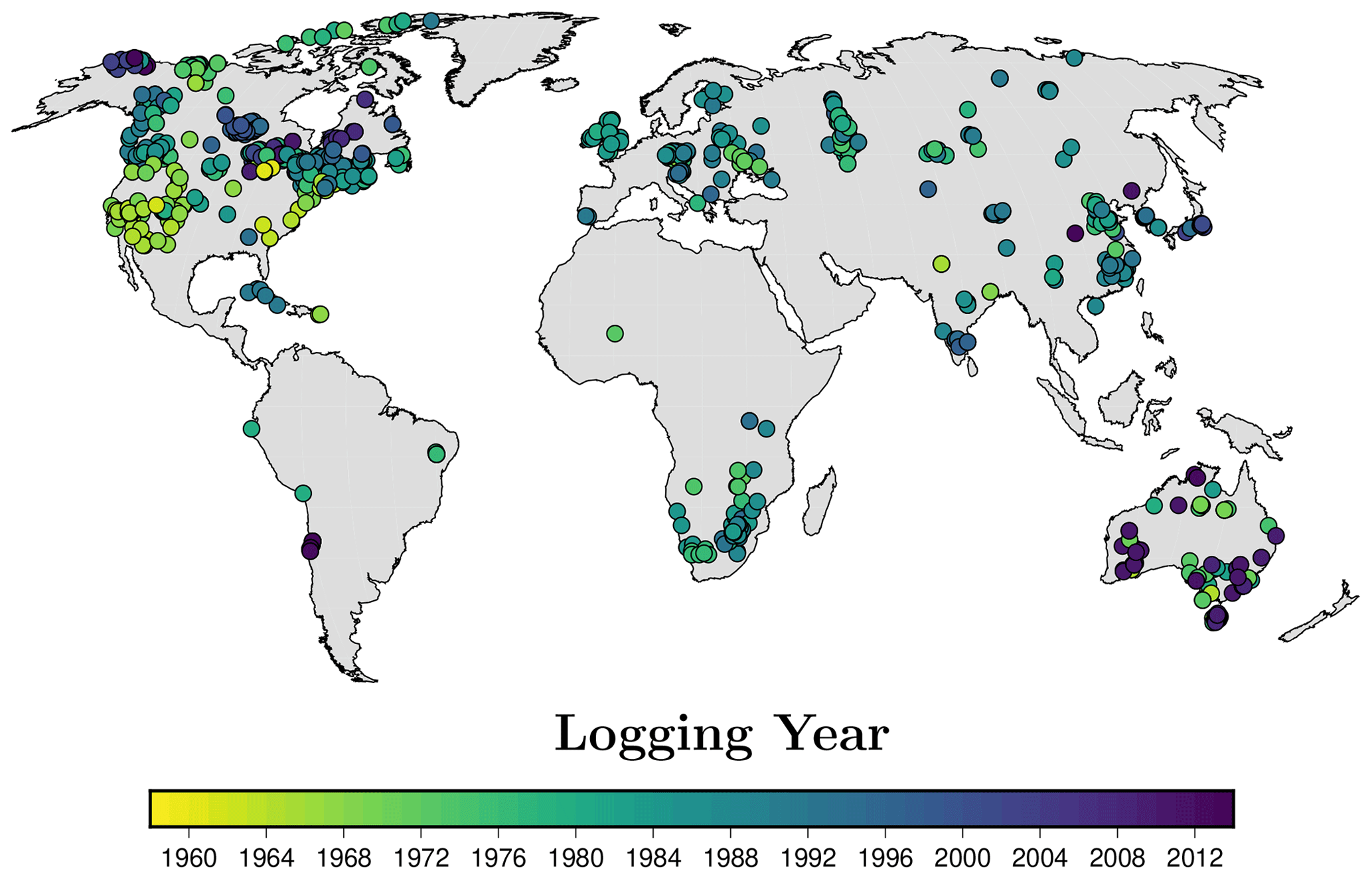
Figure 1Logging years of the 1079 boreholes considered in the analysis.
3.2 Surface air temperature data
Meteorological measurements of surface air temperature (SAT) from the Climate Research Unit (CRU) at the University of East Anglia (named SAT_CRU hereinafter) are also used in this study to compare with borehole estimates. Mean global SAT anomalies relative to 1961–1990 Common Era (CE) from the CRU TS 4.01 product (Harris et al., 2014) are employed to compare with ground surface temperature histories retrieved from borehole profiles. Results for the entire CRU spatial and temporal domains are provided from 1901 to 2016 CE, and results considering only locations and dates containing borehole inversions.
3.3 Inversion of borehole profiles
3.3.1 Standard inversions
We invert the same truncated BTPs to obtain ground surface temperature histories considering the uncertainty from the determination of the equilibrium profile as a reference to compare with the uncertainty estimates of recent works using the same SVD algorithm (Beltrami et al., 2015a; Jaume-Santero et al., 2016; Pickler et al., 2016, 2018). In this case, all logs are inverted considering a model based on a thermal conductivity of 3 W m−1 K−1, a volumetric heat capacity of 3×10⁶ J m−3 K−1, and thus a thermal diffusion of m2 s−1. The same SVD algorithm used in Beltrami (2002a) and Beltrami et al. (2002) is applied to generate the ground surface temperature histories for three step change models, since there is no preferential inversion model. All BTPs are inverted using models based on step changes of 25, 40, and 50 years to reconstruct the surface signal for 400 years before the logging date of the profile (i.e., inversion models of 16, 10, and 8 time steps, respectively), with all inversions including the four highest eigenvalues. We regard these as the GST_Standard ensemble that will serve as a reference for the methods described in Sect. 3.3.2.
The equilibrium temperature profile is estimated in order to obtain the anomaly profile that is inverted by the SVD algorithm. The equilibrium profile is estimated from the deepest part of each truncated BTP, since that is the zone least affected by the recent climate change signal (grey zone in Fig. 2a). A linear regression analysis of the lowermost 100 m of each profile (from 200 to 300 m of depth in our analysis; straight lines in Fig. 2a) is performed to estimate the values determining the quasi-equilibrium temperature profile: that is, the long-term surface temperature (T0) and the equilibrium geothermal gradient (Γ). We use the last hundred meters and not a longer depth range to reach a balance between the characterization of noise and retrieving as much climatic information as possible from each log (Beltrami et al., 2015a). The anomaly profile is then retrieved by subtracting the quasi-equilibrium temperature profile from the measured log (black dots in Fig. 2b). Additionally, the errors in the slope (Γ) and intercept (T0) allow us to obtain two extremal temperature anomaly profiles (red and blue dots in Fig. 2b). The inversion of these additional anomaly profiles is considered to be the error in the retrieved ground surface temperature histories from each borehole. We do not invert the heat flux profiles using this approach but provide surface flux estimates from the retrieved surface temperature histories to compare with Beltrami (2002a) and Beltrami et al. (2002) (see Sect. 3.4 for details).
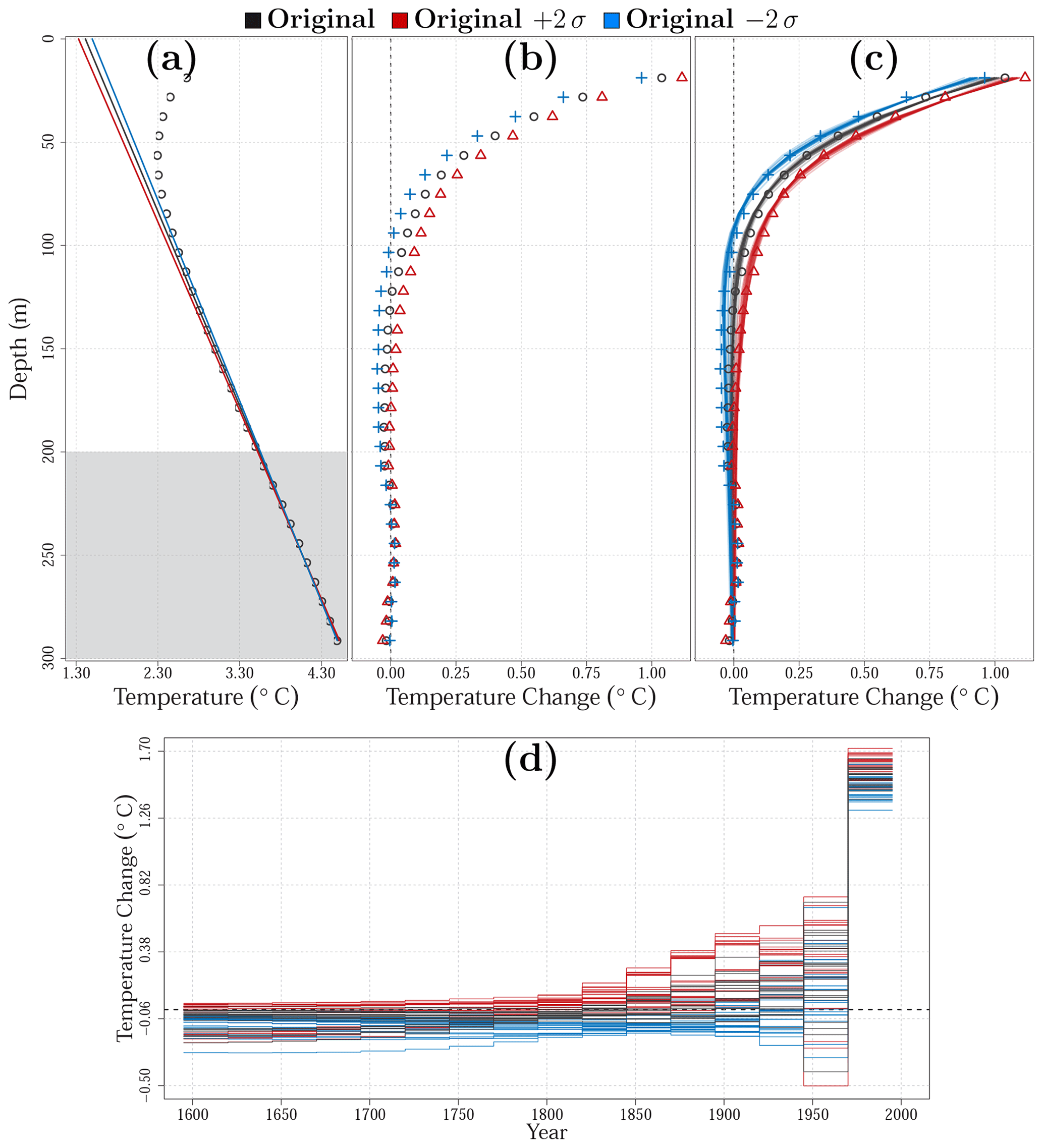
Figure 2Borehole temperature profile measurements at Fox Mine (CA_9519), Manitoba (Canada), as an example to explain the inversion approaches in this study. (a) Observed original profile (black dots), the estimated subsurface quasi-equilibrium temperature profile (black line), and the two extremal temperature profiles (red and blue lines) displaying the error in determining the quasi-equilibrium profile. All three equilibrium profiles were estimated from the linear regression analysis of the deepest part of the measured profile (from 200 to 300 m, grey zone). (b) Anomaly profiles estimated by subtracting the three equilibrium profiles from the original temperature profile. (c) As in (b), but including the 243 synthetic profiles generated from the corresponding ground surface temperature histories constituting the PPI ensemble of this borehole (red, blue and black shades). (d) Final ensemble of ground surface temperature histories considered for estimating the 5th, 50th, and 95th weighted percentiles for this borehole. Each history is weighted depending on its performance against the corresponding anomaly profile (c).
3.3.2 Perturbed parameter inversions of temperature profiles
Although the inversion approach used in previous studies was successful in retrieving the past long-term evolution of ground surface temperatures and ground heat fluxes at BTP locations, several sources of uncertainty remained unaddressed. Here, we use a new approach based on generating an ensemble of inversions using the SVD algorithm described in Mareschal and Beltrami (1992) for each borehole profile to account for as many sources of uncertainty as possible. The ensemble contains inversions retrieved by considering a range of values for the thermal properties, a different number of eigenvalues in the SVD algorithm, and the inversions of the two additional anomaly profiles generated from the estimate of the quasi-equilibrium temperature profile. Thereby, three sources of uncertainty are considered in the analysis, expanding the methodology of previous studies based on BTP inversions performed with the same SVD algorithm (Beltrami et al., 2015a; Jaume-Santero et al., 2016; Pickler et al., 2016, 2018). Additionally, all BTPs are inverted using the three different inversion models used in the standard approach. We name this new approach the perturbed parameter inversion (PPI hereinafter) due to the similarities to the generation of perturbed parameter ensembles in climate modeling (e.g., Collins et al., 2011).
The PPI approach considers the three anomaly profiles estimated from the uncertainty in determining the subsurface equilibrium profile as in the standard approach (e.g., Jaume-Santero et al., 2016, and the section above). Each of the these anomaly profiles is inverted using different values of thermal conductivity (λ) and volumetric heat capacity (ρC). The values of thermal conductivity considered in this analysis are 2.5, 3, and 3.5 W m−1 K−1, while the values for volumetric heat capacity are 2.5, 3, and 3.5×10⁶ J m−3 K−1. This includes the typical values of 3 W m−1 K−1 and 3×10⁶ J m−3 K−1 for the conductivity and heat capacity, respectively, as well as two extremal cases to account for plausible variations of thermal properties. The combination of each pair of conductivities and heat capacities yields a series of nine values for thermal diffusivity ranging between 0.7 and m2 s−1. Additionally, estimates obtained for the three inversion models use different numbers of eigenvalues to retrieve the surface signal, corresponding to the sensitivity of the SVD algorithm to small eigenvalues and to the length of each time step in the inversion model (Hartmann and Rath, 2005; Melo-Aguilar et al., 2020). Thus, inversions based on the 25-year step change model use the highest three, four, and five eigenvalues, inversions based on the 40-year step change model use the highest two, three, and four eigenvalues, and inversions based on the 50-year step change model use the highest two, three, and four eigenvalues.
Therefore, the PPI ensemble generated from each original borehole temperature profile consists of 243 different surface temperature inversions. All these inversions are then propagated using a purely conductive forward model in order to obtain synthetic BTPs as described in Eq. (5), which are compared with the original anomaly profiles (Fig. 2c). This allows us to evaluate the performance of the different parameter variants in the inversion and to attribute relative weights to them. Root mean squared errors (RMSEs) between the anomaly profiles and the synthetic profiles generated from the inversions are computed to assign a weight to each inversion following a Gaussian function as in Knutti et al. (2017):
where wi is the weight associated with the ith inversion, and σ is a parameter determining which RMSEs are deemed large and which are deemed small. We select the typical error in BTP measurements (σ=50 mK) as a criterion to assess how each inversion should be weighted: that is, to evaluate which RMSEs are large and which are small.
Thus, each inversion is classified according to the realism of its associated synthetic anomaly profile. Nevertheless, unrealistic solutions may arise as a result of the broad range of parameters and inversion models considered, even after weighting each inversion. Hence, we introduce a new additional criterion to assess all 243 inversions per BTP based on the variability of surface air temperature measurements as a guide. A temperature change in an inverted ground surface temperature history is considered unrealistic if it is larger than the maximum change obtained from the histogram of temperature variations between consecutive time steps from the SAT_CRU data. This histogram is created by aggregating temperature changes between consecutive time steps after averaging the original temperature series at each grid cell in temporal windows of 25 years (i.e., running means of 25 years; Fig. S1). The averaging of the original temperature series is necessary to remove high-frequency variability that is not present in ground surface temperature histories from BTP inversions. That is, a ground surface temperature history is deemed unrealistic and removed from the analysis if the temperature change between at least one pair of consecutive time steps is larger than 2.57 K for the three inversion models. The 5th, 50th, and 95th weighted percentiles are eventually estimated from the ensemble of remaining inversions (Fig. 2d) for each borehole profile. The ensemble containing the weighted percentiles from ground surface temperature histories from all BTPs is called the GST_PPIT ensemble hereinafter.
3.3.3 Perturbed parameter inversions of heat flux profiles
The same approach is applied to the corresponding heat flux profiles to retrieve ground heat flux histories from borehole data. The heat flux profiles are generated from the three estimated temperature anomaly profiles for each measured log using Fourier's equation (Eq. 6) as
Those profiles are then inverted using the PPI approach described above. That is, an ensemble of inversions is generated using the same SVD algorithm, the same range of thermal properties, and the same number of eigenvalues as for the GST_PPIT ensemble in Sect. 3.3.2. Thus, the thermal conductivity for estimating the heat flux profile (λ in Eq. 17) is set to match the values used for each perturbed parameter inversion. Thereby, we obtain 243 heat flux histories for each original log, which are compared to the corresponding flux anomaly profile (using Eq. 10) and weighted as in the case of temperature histories (Eq. 16). Changes in ground heat flux histories are compared to the histogram created by aggregating heat flux changes estimated from the CRU temperature data and Eq. (18) (GHF_CRU hereinafter) in order to discard unrealistic heat flux histories. As in the case of temperature changes, heat flux changes between consecutive time steps are aggregated after averaging the original heat flux series from each grid cell over temporal windows of 25 years (Fig. S1). Surface heat flux histories are deemed unrealistic if the difference between at least one pair of consecutive time steps is larger than 0.51 W m−2 for the three inversion models. The ensemble containing the 5th, 50th, and 95th weighted percentiles from ground heat flux histories from all BTPs is called the GHF_PPIF ensemble hereinafter.
Estimates from temperature profiles and from heat flux profiles using the PPI and standard approaches need to include inversions from the same number of BTPs to obtain the same geographical representation of surface temperature and heat flux changes. This requirement reduces the number of boreholes considered in the analysis to 1060, 1072, and 1074 for the 25-, 40-, and 50-year inversion models, respectively, since not all BTPs provide ground surface temperature histories and ground heat flux histories complying with all criteria explained in Sect. 3.3.2 and 3.3.3, respectively.
3.4 Flux estimates from surface temperatures
The relationship between surface flux (q) and a temporal series of surface temperatures can be expressed as (Wang and Bras, 1999; Beltrami, 2001)
where Δt is the length of the time steps and Ti is surface temperature at the ith time step. We estimate ground heat flux histories at the surface from ground surface temperature histories retrieved from both the standard (GHF_Standard ensemble) and PPI approaches (GHF_PPIT ensemble). Thermal properties for estimating heat fluxes from ground surface temperature histories obtained with the standard inversion approach are set to λ=3 W m−1 K−1 and m2 s−1, while thermal properties for estimating heat fluxes from ground surface temperature histories included in the GST_PPIT ensemble are set as those associated with the corresponding individual ground surface temperature history. Heat flux estimates are also provided using Eq. (18) and SAT_CRU temperature data (GHF_CRU ensemble mentioned in Sect. 3.3.3) in order to create the histogram of heat flux changes displayed in Fig. S1, considering the same thermal properties as in heat flux estimates from ground surface temperature histories retrieved by the standard approach.
Ground surface temperature histories estimated using a 25-year inversion model, together with the standard approach and the new GST_PPIT ensemble, show temperature increases that are particularly large during the second half of the 20th century in comparison with preindustrial conditions (Fig. 3a). This is in agreement with meteorological observations of surface air temperatures (red and orange lines in the mentioned figure) and with previous studies using both borehole temperature profiles and proxy data (Pollack et al., 1998; Huang et al., 2000; Beltrami, 2002a; Pollack and Smerdon, 2004; Fernández-Donado et al., 2013; Masson-Delmotte et al., 2013). Both approaches used to retrieve ground surface temperature histories from temperature profiles display remarkable agreement during the whole period and similar temperature changes as those shown by SAT_CRU temperatures for the observational period. Global mean temperature changes between 1950–1975 and 1975–2000 CE reach 0.3 K for the GST_PPIT ensemble and 0.4 K for the GST_Standard ensemble (Table 1), with mean temperature changes from SAT_CRU data of approximately 0.4 K using both the entire dataset and the locations and dates containing BTP inversions.

Figure 3Global ground surface temperature histories (a) and global ground heat flux histories at the surface (b) from borehole temperature profiles using the standard approach (black) and the new PPI approach applied to temperature profiles (PPIT, blue) and the corresponding heat flux profiles (PPIF, light blue). All inversions were performed using a 25-year step change model. (c) Percentage of total borehole inversions with time. Surface air temperature anomalies relative to 1961–1990 CE from CRU data (SAT_CRU) are also displayed, including results from the entire database (red) and results from locations and dates containing borehole inversions (orange). The CRU series have been adjusted to have the same mean as the results of the GST_Standard ensemble for the period 1950–1970 CE.
Table 1Global mean estimates of ground surface temperature (GST), ground heat flux at the surface (GHF), and ground heat content within the continental subsurface (GHC) from borehole temperature profiles. Values display the mean and 95 % confidence interval for each time period from estimates using the standard inversion approach (standard) and the new PPI approach applied to temperature and heat flux profiles (PPIT and PPIF, respectively). All the inversions were performed using a model of 25 years per time step (temperatures: K; fluxes: mW m−2; heat content: ZJ).
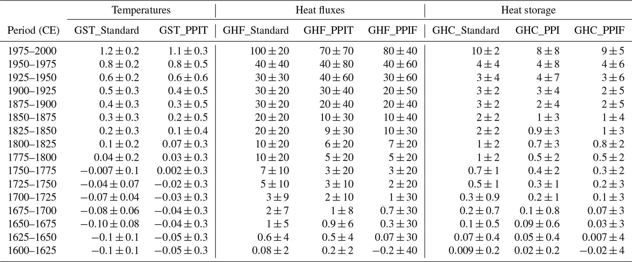
Ground surface temperature histories present slightly higher temperature changes since preindustrial times than previously reported, with results ranging from 1.0±0.1 K to 1.2±0.2 K for the last part of the 20th century considering results from the three inversion models (Tables 1, S1, and S2) in comparison to the ∼0.9 K reported in previous works (Huang et al., 2000; Harris and Chapman, 2001; Beltrami, 2002a; Pollack and Smerdon, 2004). Furthermore, ground surface temperature histories show a temperature increase of around 0.5±0.3 K using the GST_Standard ensemble and 0.3±0.5 K using the GST_PPIT ensemble at the beginning of the instrumental period relative to preindustrial times (∼1900 CE; Fig. 3a). Thus, 67 % and 81 % of the land warming occurs after 1900 CE in the GST_Standard ensemble and the GST_PPIT ensemble, respectively, indicating an accelerated land warming during the 20th century, in agreement with other reconstructions of past changes in surface temperature (Masson-Delmotte et al., 2013).
As in the case of surface temperature histories, the three approaches providing ground heat flux histories from BTP measurements are in good agreement during the entire period, although they present higher uncertainties than for temperatures (Fig. 3b and Table 1). Global results from Beltrami et al. (2002) are also displayed in Fig. 3b (purple line), reaching similar values in comparison with ground heat flux histories in the GHF_Standard, GHF_PPIT, and GHF_PPIF ensembles except for the second half of the 20th century. Global heat flux change reaches 70±20, 60±50, and 60±40 mW m−2 for the GHF_Standard, GHF_PPIT, and GHF_PPIF ensembles, respectively (Table 1), in contrast to 39±4 mW m−2 presented in Beltrami et al. (2002) and ∼33 mW m−2 from Beltrami (2002a). The large number of recently acquired profiles included in our analysis may explain the larger flux estimates in comparison with previous works, since BTP measurements recorded before the 1980s did not capture the large disturbances in the surface energy budget from recent decades (Stevens et al., 2008). Global changes in ground heat content were estimated from the GHF_Standard, GHF_PPIT, and GHF_PPIF ensembles by scaling these fluxes to the continental areas except Antarctica and Greenland, where there are no BTP measurements, which results in three new sets of results: the GHC_Standard, GHC_PPIT, and GHC_PPIF ensembles. Changes in ground heat content of 15±5, 10±10, and 13±8 ZJ (1 ZJ = 1021 J) are obtained for the period 1950–2000 CE using the GHC_Standard, GHC_PPIT, and GHC_PPIF ensembles, respectively, in comparison with 9±1 ZJ in Beltrami et al. (2002) and 7 ZJ in Beltrami (2002a). As expected, these estimates of continental heat storage are larger than previously reported since the heat flux histories also present higher values. The small uncertainty for heat flux histories, and therefore for estimates of continental heat storage, shown by the standard and PPI approaches at the beginning of the period (Fig. 3) is artificially imposed by Eq. (18), since the heat flux estimate for the first temporal step is set to zero by default. Therefore, the GHF_PPIF and GHC_PPIF ensembles provide a more realistic estimate of the uncertainty in the global ground heat flux histories and ground heat content estimates for the first half of the period, with larger uncertainties for all ensembles in the second half of the period.
Although the borehole database used here contains BTP measurements recorded after 2000 CE, results are shown until the end of the 20th century, since the number of available logs decreases sharply afterwards and the remaining profiles are located mainly at high latitudes in North America and Australia (Fig. 1). We use the trend for the period 1970–2000 CE to extrapolate the heat flux histories until 2018 CE, providing an estimate of the accumulated heat content in the continental subsurface from 1960 CE to the present (Fig. 4). The global mean change in heat flux for the entire period is approximately 90 mW m−2 considering all inversion approaches, while the global heat flux change since 2000 CE is ∼120 mW m−2. Thus, the accumulated heat within the global continental subsurface obtained from these flux estimates reaches 20 ZJ for the entire period and ∼9 ZJ for 2000–2018 CE. That is, if the global heat flux increase during the first decades of the 21st century resembled the trend of the period 1970–2000 CE, half of the total increase in energy storage within the continental subsurface in the last 58 years would have occurred during the last 2 decades, a remarkably similar result in comparison with the accelerated ocean heat uptake in the last decades (Gleckler et al., 2016; Cheng et al., 2017, 2019).
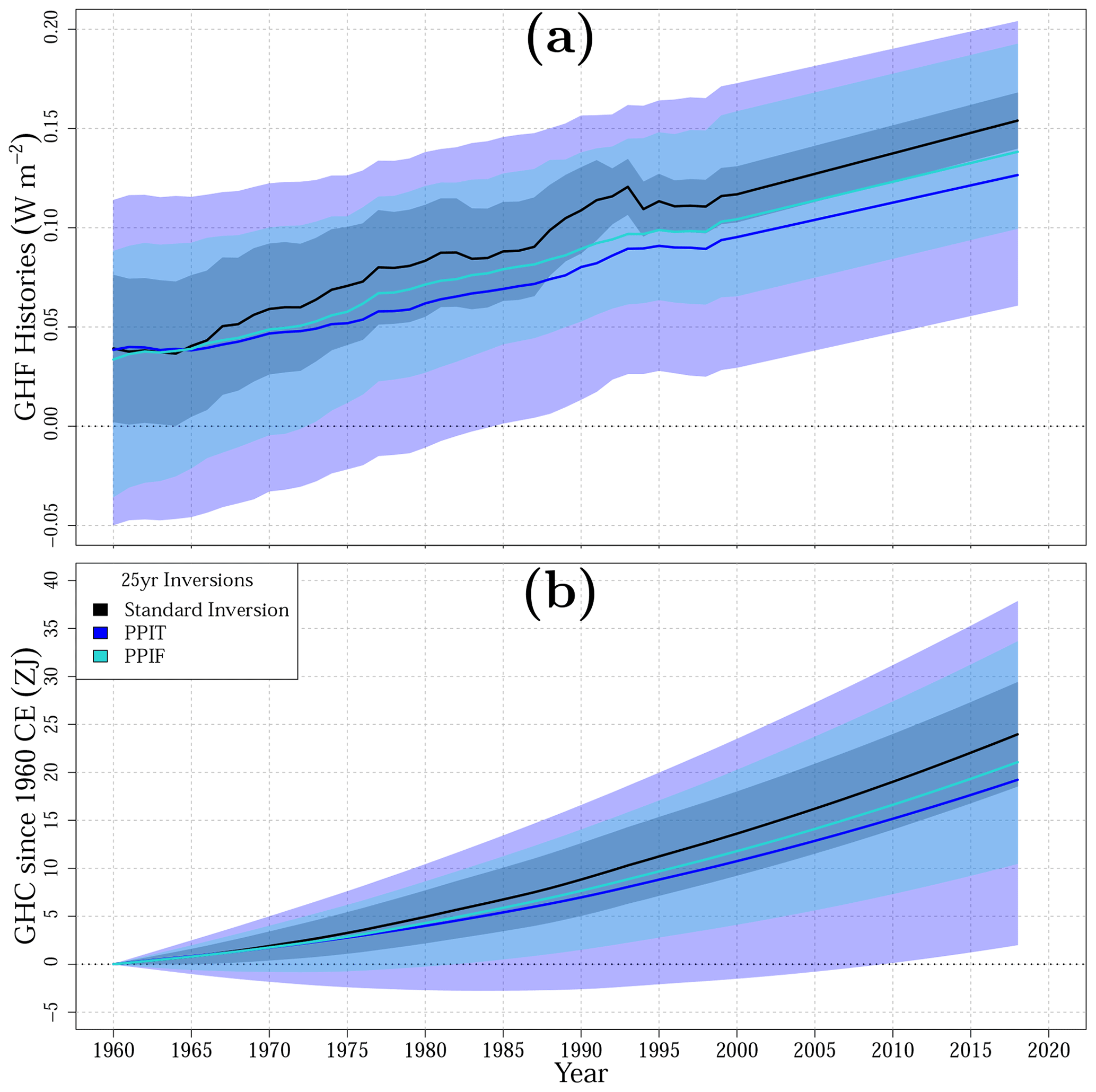
Figure 4Global ground heat flux histories (a) and ground heat content accumulated since 1960 CE (b) from borehole temperature profiles using the standard approach (black) and the new PPI approach applied to temperature profiles (PPIT, blue) and the corresponding heat flux profiles (PPIF, light blue). All inversions were performed using a 25-year inversion model. Data for 2001 to 2018 CE are extrapolated using the trend for the period 1971–2000 CE.
Ground surface temperature and ground heat flux histories retrieved by the three inversion models used here show similar evolutions since preindustrial times and yield similar estimates of ground heat content for all continental areas without considering Antarctica and Greenland (Figs. 3, S2, and S3; Tables 1, S1, and S2). Nonetheless, the surface temperature, heat flux, and heat storage results are larger than previous global estimates of ground surface temperature histories, ground heat flux histories, and ground heat content from borehole data (Pollack et al., 1998; Huang et al., 2000; Beltrami, 2002a; Beltrami et al., 2002; Pollack and Smerdon, 2004). The main reason for the higher values reported here is the inclusion of additional temperature profiles measured at more recent dates than those employed in the literature, since logs acquired after the 1980s and 1990s recorded larger changes in the subsurface thermal regime due to larger variations in the surface energy balance (Stevens et al., 2008). That is, more than 250 high-quality logs have been measured or made available for the community since the early 2000s, including profiles from scarcely represented areas in the Southern Hemisphere. Additionally, there have been improvements in the aggregation and treatment of borehole profiles, contributing to the differences between our estimates and previous works (Beltrami et al., 2015b). We have truncated all logs to the same depth before performing the analysis in contrast to previous studies, which used profiles including a range of bottom depths, therefore including estimates of ground surface temperature histories and ground heat flux histories with different periods of reference.
The larger differences in uncertainties in heat flux estimates from the GHF_PPIT ensemble in comparison with those from the GHF_PPIF ensemble are caused by the criteria to discard unrealistic inversions in the PPI approach (Figs. 3b, S2b, and S3b). That is, the heat flux estimates for the GHF_PPIT ensemble were not filtered out using the flux criterion (0.51 W m−2) of the PPI approach but the temperature criterion (2.57 K). Applying these different criteria is necessary since heat flux estimates from the GHF_PPIT ensemble result from applying Eq. (18) to the previously retrieved surface temperature histories in the GST_PPIT ensemble, while the heat flux histories considered in the GHF_PPIF ensemble result from direct inversions of heat flux profiles, as explained in Sect. 3.3.3.
Borehole temperature profiles demonstrate a unique ability to integrate multi-centennial changes in the surface energy balance (Beltrami, 2002b), which makes borehole inversions an important source of information about preindustrial conditions. The depth range considered here (from 15 to 300 m) allows us to retrieve information from ∼700 years before the logging date of each log, i.e., several centuries before industrialization. Thus, all surface temperature histories displayed in Figs. 3a, S2a, and S3a are relative to approximately 1300–1700 CE, as the subsurface quasi-equilibrium profile is estimated here from the 200–300 m depth range for all profiles (Cuesta-Valero et al., 2019). The ground surface temperature increases relative to preindustrial conditions from the three GST_PPIT ensembles analyzed here are ∼1.0 K for the last part of the 20th century, as previously shown in the Results section and Tables 1, S1, and S2. This is not, however, an estimate of the global temperature change, since land temperature changes at a higher pace than the temperature at the surface of the ocean due to their different thermal properties. The ratio between land temperature change and ocean temperature change is estimated in Harrison et al. (2015) based on an ensemble of long-term general circulation model simulations performed under different external forcings, resulting in land temperature changes ∼2.36 times larger than ocean temperature changes. Thus, the ocean temperature change corresponding to the land temperature change retrieved from borehole temperature profiles can be approximated as ∼0.4 K, which suggests a global temperature change of ∼0.7 K since preindustrial times. Such a temperature change from preindustrial conditions is in good agreement with the estimates of 0.55–0.8 K discussed in Hawkins et al. (2017) using observations, general circulation model simulations, and proxy databases, even for a preindustrial period much further in the past in comparison with the periods analyzed in Schurer et al. (2017).
These new estimates of continental heat storage and ground heat flux from BTP inversions have implications for the assessment of the Earth's heat inventory and for comparison with general circulation model simulations. The ocean heat flux is still much larger than the ground heat flux, with an ocean flux of mW m−2 (von Schuckmann et al., 2020) in contrast to the mW m−2 ground heat flux (Fig. 4) for the period 1993–2018 CE. Nevertheless, although the ocean is still the largest component of the Earth's heat inventory (89 %), the contribution of the continental subsurface is higher than previously reported (6 % instead of 2 %–5 %; von Schuckmann et al., 2020), reinforcing the necessity of monitoring and accounting for the rest of the components in the inventory. Furthermore, previous assessments have shown that general circulation model simulations are unable to represent changes in continental heat storage due to their shallow land surface model components (Stevens et al., 2007; MacDougall et al., 2008; Cuesta-Valero et al., 2016). The new estimates of continental heat storage emphasize the demand for deeper subsurfaces in general circulation models in order to generate global transient simulations capable of correctly reproducing the Earth's heat inventory.
The distribution of BTP measurements used in this analysis is especially scarce in zones of Africa, South America, and the Middle East, which may raise doubts about the global representativity of the assembled borehole dataset. Previous works have assessed the spatial distribution of BTP measurements using transient climate simulations performed by general circulation models at millennial timescales (González-Rouco et al., 2006, 2009; García-García et al., 2016; Melo-Aguilar et al., 2020) and borehole databases aggregated using different techniques (Beltrami and Bourlon, 2004; Pollack and Smerdon, 2004), with all studies concluding that the effects of limited regional sampling on estimates of global changes should be minor. Additionally, surface air temperatures from SAT_CRU data present markedly similar values considering both the full domain and the locations and dates containing BTP inversions (see red and orange lines in Fig. 3), supporting the claim that borehole temporal and spatial distributions are representative of global conditions. Nevertheless, repeating measurements at previously logged borehole sites and obtaining new records at zones with a reduced density of BTP data would improve the global estimates of ground surface temperature and ground heat flux histories from borehole temperature profiles.
The magnitude of the retrieved changes in ground surface temperature in this analysis supports the claim that the Earth's surface has warmed by ∼0.7 K since preindustrial times. The new estimates also reveal that the continental subsurface stored more energy during the last part of the 20th century than previously reported, reaching around 12 ZJ. This evidences the need to include deeper land surface model components in transient simulations performed by general circulation models in order to correctly reproduce the land component of the Earth's heat inventory and potentially powerful carbon feedbacks related to energy-dependent processes of the continental subsurface, such as the stability of the soil carbon pool and permafrost evolution.
| Acronym | Definition |
| BTP | Borehole temperature profile |
| CE | Common Era |
| PPI | Perturbed parameter inversion |
| GST_PPIT | Ground surface temperature (GST) retrieved using the perturbed parameter inversion (PPI) approach and subsurface |
| temperature profiles (Sect. 3.3.2) | |
| GST_Standard | Ground surface temperature (GST) retrieved using the standard approach (Sect. 3.3.1) |
| GHF_PPIF | Ground heat flux (GHF) at the surface retrieved using the perturbed parameter inversion (PPI) approach and subsurface |
| flux profiles (Sect. 3.3.3) | |
| GHF_PPIT | Ground heat flux (GHF) at the surface retrieved using the GST_PPIT ensemble and Eq. (18) |
| GHF_Standard | Ground heat flux (GHF) at the surface retrieved using the GST_Standard ensemble and Eq. (18) |
| GHC_PPIF | Ground heat content (GHC) retrieved using the GHF_PPIF ensemble |
| GHC_PPIT | Ground heat content (GHC) retrieved using the GHF_PPIT ensemble |
| GHC_Standard | Ground heat content (GHC) retrieved using the GHF_Standard ensemble |
| RMSE | Root mean square error |
| SAT_CRU | Surface air temperature (SAT) from CRU TS 4.01 product |
| SVD | Singular value decomposition |
Data from the Climatic Research Unit (CRU) at the University of East Anglia can be accessed at https://doi.org/10/gcmcz3 (University of East Anglia Climatic Research Unit et al., 2017). Borehole data can be found on the Figshare repository at https://doi.org/10.6084/m9.figshare.13516487 (Cuesta-Valero et al., 2021).
The supplement related to this article is available online at: https://doi.org/10.5194/cp-17-451-2021-supplement.
FJCV analyzed the borehole data, developed the PPI technique that was applied to characterize uncertainties in borehole inversions, and produced all results and figures. FJCV, AGG, HB, JFGR, and EGB contributed to the interpretation and discussion of results. FJCV wrote the first version of the paper, with subsequent contributions from AGG, HB, JFGR, and EGB to all sections.
The authors declare that they have no conflict of interest.
We are grateful for two anonymous reviewers and their thoughtful and constructive feedback. This analysis contributes to the PALEOLINK project (http://pastglobalchanges.org/science/wg/2knetwork/projects/paleolink/intro, last access: 16 February 2021), part of the PAGES 2k Network. Hugo Beltrami was supported by the Natural Sciences and Engineering Research Council of Canada, the Canada Research Chairs Program, and the Canada Foundation for Innovation. Hugo Beltrami holds the Canada Research Chair in Climate Dynamics. Almudena García-García and Francisco José Cuesta-Valero were funded by Hugo Beltrami's Canada Research Chair program, the School of Graduate Students at the Memorial University of Newfoundland, and the Research Office at St. Francis Xavier University.
This research has been supported by the Natural Sciences and Engineering Research Council of Canada (grant no. NSERC DG 140576948) and the Canada Research Chairs (grant no. CRC 230687).
This paper was edited by Nerilie Abram and reviewed by two anonymous referees.
Barkaoui, A. E., Correia, A., Zarhloule, Y., Rimi, A., Carneiro, J., Boughriba, M., and Verdoya, M.: Reconstruction of remote climate change from borehole temperature measurement in the eastern part of Morocco, Climatic Change, 118, 431–441, https://doi.org/10.1007/s10584-012-0638-7, 2013. a
Beck, A.: Climatically perturbed temperature gradients and their effect on regional and continental heat-flow means, Tectonophysics, 41, 17–39, https://doi.org/10.1016/0040-1951(77)90178-0, 1977. a
Beltrami, H.: Surface heat flux histories from inversion of geothermal data: Energy balance at the Earth's surface, J. Geophys. Res.-Sol. Ea., 106, 21979–21993, https://doi.org/10.1029/2000JB000065, 2001. a, b, c
Beltrami, H.: Climate from borehole data: Energy fluxes and temperatures since 1500, Geophys. Res. Lett., 29, 26-1–26-4, https://doi.org/10.1029/2002GL015702, 2002a. a, b, c, d, e, f, g, h, i, j
Beltrami, H.: Earth's Long-Term Memory, Science, 297, 206–207, https://doi.org/10.1126/science.1074027, 2002b. a, b
Beltrami, H. and Bourlon, E.: Ground warming patterns in the Northern Hemisphere during the last five centuries, Earth Planet. Sc. Lett., 227, 169–177, https://doi.org/10.1016/j.epsl.2004.09.014, 2004. a, b
Beltrami, H., Jessop, A. M., and Mareschal, J.-C.: Ground temperature histories in eastern and central Canada from geothermal measurements: evidence of climatic change, Global Planet. Change, 6, 167–183, https://doi.org/10.1016/0921-8181(92)90033-7, 1992. a
Beltrami, H., Smerdon, J. E., Pollack, H. N., and Huang, S.: Continental heat gain in the global climate system, Geophys. Res. Lett., 29, 8-1–8-3, https://doi.org/10.1029/2001GL014310, 2002. a, b, c, d, e, f, g, h, i
Beltrami, H., Bourlon, E., Kellman, L., and González-Rouco, J. F.: Spatial patterns of ground heat gain in the Northern Hemisphere, Geophys. Res. Lett., 33, l06717, https://doi.org/10.1029/2006GL025676, 2006. a, b
Beltrami, H., Matharoo, G. S., and Smerdon, J. E.: Ground surface temperature and continental heat gain: uncertainties from underground, Environ. Res. Lett., 10, 014009, https://doi.org/10.1088/1748-9326/10/1/014009, 2015a. a, b, c, d
Beltrami, H., Matharoo, G. S., and Smerdon, J. E.: Impact of borehole depths on reconstructed estimates of ground surface temperature histories and energy storage, J. Geophys. Res.-Earth, 120, 763–778, https://doi.org/10.1002/2014JF003382, 2014JF003382, 2015b. a, b, c
Beltrami, H., Matharoo, G. S., Smerdon, J. E., Illanes, L., and Tarasov, L.: Impacts of the Last Glacial Cycle on ground surface temperature reconstructions over the last millennium, Geophys. Res. Lett., 44, 355–364, https://doi.org/10.1002/2016GL071317, 2017. a, b
Bodri, L. and Cermak, V.: Borehole temperatures, climate change and the pre-observational surface air temperature mean: allowance for hydraulic conditions, Global Planet. Change, 45, 265–276, https://doi.org/10.1016/j.gloplacha.2004.09.001, 2005. a
Bullard, E. C. and Schonland, B. F. J.: Heat flow in South Africa, P. Roy. Soc. Lond. A Mat., 173, 474–502, https://doi.org/10.1098/rspa.1939.0159,1939. a
Campbell, B. M., Vermeulen, S. J., Aggarwal, P. K., Corner-Dolloff, C., Girvetz, E., Loboguerrero, A. M., Ramirez-Villegas, J., Rosenstock, T., Sebastian, L., Thornton, P. K., and Wollenberg, E.: Reducing risks to food security from climate change, Global Food Security, 11, 34–43, https://doi.org/10.1016/j.gfs.2016.06.002, 2016. a
Carslaw, H. and Jaeger, J.: Conduction of Heat in Solids, Clarendon Press, Oxford, 1959. a, b, c, d, e
Cermak, V.: Underground temperature and inferred climatic temperature of the past millenium, Palaeogeography, Palaeoclimatology, Palaeoecology, 10, 1–19, https://doi.org/10.1016/0031-0182(71)90043-5, 1971. a
Cheng, L., Trenberth, K. E., Fasullo, J., Boyer, T., Abraham, J., and Zhu, J.: Improved estimates of ocean heat content from 1960 to 2015, Sci. Adv., 3, e1601545, https://doi.org/10.1126/sciadv.1601545, 2017. a
Cheng, L., Abraham, J., Hausfather, Z., and Trenberth, K. E.: How fast are the oceans warming?, Science, 363, 128–129, https://doi.org/10.1126/science.aav7619, 2019. a
Chouinard, C. and Mareschal, J.-C.: Ground surface temperature history in southern Canada: Temperatures at the base of the Laurentide ice sheet and during the Holocene, Earth Planet. Sci. Lett., 277, 280–289, https://doi.org/10.1016/j.epsl.2008.10.026, 2009. a
Church, J. A., White, N. J., Konikow, L. F., Domingues, C. M., Cogley, J. G., Rignot, E., Gregory, J. M., van den Broeke, M. R., Monaghan, A. J., and Velicogna, I.: Revisiting the Earth's sea-level and energy budgets from 1961 to 2008, Geophys. Res. Lett., 38, l18601, https://doi.org/10.1029/2011GL048794, 2011. a, b
Clauser, C. and Mareschal, J.-C.: Ground temperature history in central Europe from borehole temperature data, Geophys. J. Int., 121, 805–817, https://doi.org/10.1111/j.1365-246X.1995.tb06440.x, 1995. a
Collins, M., Booth, B. B. B., Bhaskaran, B., Harris, G. R., Murphy, J. M., Sexton, D. M. H., and Webb, M. J.: Climate model errors, feedbacks and forcings: a comparison of perturbed physics and multi-model ensembles, Clim. Dyn., 36, 1737–1766, https://doi.org/10.1007/s00382-010-0808-0, 2011. a
Cuesta-Valero, F. J., García-García, A., Beltrami, H., and Smerdon, J. E.: First assessment of continental energy storage in CMIP5 simulations, Geophys. Res. Lett., 43, 2016GL068496, https://doi.org/10.1002/2016GL068496, 2016. a, b
Cuesta-Valero, F. J., García-García, A., Beltrami, H., Zorita, E., and Jaume-Santero, F.: Long-term Surface Temperature (LoST) database as a complement for GCM preindustrial simulations, Clim. Past, 15, 1099–1111, https://doi.org/10.5194/cp-15-1099-2019, 2019. a, b, c
Cuesta-Valero, F. J., Beltrami, H., García-García, A., González-Rourco, J. F., and García-Bustamante, E.: Xibalbá: Underground Temperature Database, Figshare, https://doi.org/https://doi.org/10.6084/m9.figshare.13516487, 2021. a, b
Davis, M. G., Harris, R. N., and Chapman, D. S.: Repeat temperature measurements in boreholes from northwestern Utah link ground and air temperature changes at the decadal time scale, J. Geophys. Res.-Sol. Ea., 115, B05203, https://doi.org/10.1029/2009JB006875, 2010. a
Demezhko, D. Y. and Gornostaeva, A. A.: Late Pleistocene–Holocene ground surface heat flux changes reconstructed from borehole temperature data (the Urals, Russia), Clim. Past, 11, 647–652, https://doi.org/10.5194/cp-11-647-2015, 2015. a
Dutton, A., Carlson, A. E., Long, A. J., Milne, G. A., Clark, P. U., DeConto, R., Horton, B. P., Rahmstorf, S., and Raymo, M. E.: Sea-level rise due to polar ice-sheet mass loss during past warm periods, Science, 349, aaa4019, https://doi.org/10.1126/science.aaa4019, 2015. a
Fernández-Donado, L., González-Rouco, J. F., Raible, C. C., Ammann, C. M., Barriopedro, D., García-Bustamante, E., Jungclaus, J. H., Lorenz, S. J., Luterbacher, J., Phipps, S. J., Servonnat, J., Swingedouw, D., Tett, S. F. B., Wagner, S., Yiou, P., and Zorita, E.: Large-scale temperature response to external forcing in simulations and reconstructions of the last millennium, Clim. Past, 9, 393–421, https://doi.org/10.5194/cp-9-393-2013, 2013. a, b
García-García, A., Cuesta-Valero, F. J., Beltrami, H., and Smerdon, J. E.: Simulation of air and ground temperatures in PMIP3/CMIP5 last millennium simulations: implications for climate reconstructions from borehole temperature profiles, Environ. Res. Lett., 11, 044022, https://doi.org/10.1088/1748-9326/11/4/044022, 2016. a, b, c
Gleckler, P. J., Durack, P. J., Stouffer, R. J., Johnson, G. C., and Forest, C. E.: Industrial-era global ocean heat uptake doubles in recent decades, Nat. Clim. Change, 6, 394–398, https://doi.org/10.1038/nclimate2915, 2016. a
González-Rouco, J. F., Beltrami, H., Zorita, E., and von Storch, H.: Simulation and inversion of borehole temperature profiles in surrogate climates: Spatial distribution and surface coupling, Geophys. Res. Lett., 33, l01703, https://doi.org/10.1029/2005GL024693, 2006. a, b
González-Rouco, J. F., Beltrami, H., Zorita, E., and Stevens, M. B.: Borehole climatology: a discussion based on contributions from climate modeling, Clim. Past, 5, 97–127, https://doi.org/10.5194/cp-5-97-2009, 2009. a, b, c, d, e
Hansen, J., Sato, M., Kharecha, P., and von Schuckmann, K.: Earth's energy imbalance and implications, Atmos. Chem. Phys., 11, 13421–13449, https://doi.org/10.5194/acp-11-13421-2011, 2011. a, b
Harris, I., Jones, P., Osborn, T., and Lister, D.: Updated high-resolution grids of monthly climatic observations – the CRU TS3.10 Dataset, Int. J. Clim., 34, 623–642, https://doi.org/10.1002/joc.3711, 2014. a
Harris, R. N. and Chapman, D. S.: Mid-latitude (30∘–60∘ N) climatic warming inferred by combining borehole temperatures with surface air temperatures, Geophys. Res. Lett., 28, 747–750, https://doi.org/10.1029/2000GL012348, 2001. a, b
Harrison, S. P., Bartlein, P. J., Izumi, K., Li, G., Annan, J., Hargreaves, J., Braconnot, P., and Kageyama, M.: Evaluation of CMIP5 palaeo-simulations to improve climate projections, Nat. Clim. Change, 5, 735–743, https://doi.org/10.1038/nclimate2649, 2015. a
Hartmann, A. and Rath, V.: Uncertainties and shortcomings of ground surface temperature histories derived from inversion of temperature logs, J. Geophys. Eng., 2, 299–311, https://doi.org/10.1088/1742-2132/2/4/S02, 2005. a, b, c, d
Hawkins, E., Ortega, P., Suckling, E., Schurer, A., Hegerl, G., Jones, P., Joshi, M., Osborn, T. J., Masson-Delmotte, V., Mignot, J., Thorne, P., and van Oldenborgh, G. J.: Estimating Changes in Global Temperature since the Preindustrial Period, B. Am. Meteorol. Soc., 98, 1841–1856, https://doi.org/10.1175/BAMS-D-16-0007.1, 2017. a
Hicks Pries, C. E., Castanha, C., Porras, R. C., and Torn, M. S.: The whole-soil carbon flux in response to warming, Science, 355, 1420–1423, https://doi.org/10.1126/science.aal1319, 2017. a
Hopcroft, P. O., Gallagher, K., and Pain, C. C.: Inference of past climate from borehole temperature data using Bayesian Reversible Jump Markov chain Monte Carlo, Geophys. J. Int., 171, 1430–1439, https://doi.org/10.1111/j.1365-246X.2007.03596.x, 2007. a
Huang, S., Pollack, H. N., and Shen, P.-Y.: Temperature trends over the past five centuries reconstructed from borehole temperatures, Nature, 403, 756–758, https://doi.org/10.1038/35001556, 2000. a, b, c, d, e
Irving, D. B., Wijffels, S., and Church, J. A.: Anthropogenic Aerosols, Greenhouse Gases, and the Uptake, Transport, and Storage of Excess Heat in the Climate System, Geophys. Res. Lett., 46, 4894–4903, https://doi.org/10.1029/2019GL082015, 2019. a, b
Jacob, T., Wahr, J., Pfeffer, W. T., and Swenson, S.: Recent contributions of glaciers and ice caps to sea level rise, Nature, 482, 514–518, https://doi.org/10.1038/nature10847, 2012. a
Jaume-Santero, F., Pickler, C., Beltrami, H., and Mareschal, J.-C.: North American regional climate reconstruction from ground surface temperature histories, Clim. Past, 12, 2181–2194, https://doi.org/10.5194/cp-12-2181-2016, 2016. a, b, c, d, e, f, g, h
Johnson, G. C., Lyman, J. M., and Loeb, N. G.: Improving estimates of Earth's energy imbalance, Nat. Clim. Change, 6, 639, https://doi.org/10.1038/nclimate3043, 2016. a
Knutti, R., Sedláček, J., Sanderson, B. M., Lorenz, R., Fischer, E. M., and Eyring, V.: A climate model projection weighting scheme accounting for performance and interdependence, Geophys. Res. Lett., 44, 1909–1918, https://doi.org/10.1002/2016GL072012, 2017. a
Kundzewicz, Z. W., Kanae, S., Seneviratne, S. I., Handmer, J., Nicholls, N., Peduzzi, P., Mechler, R., Bouwer, L. M., Arnell, N., Mach, K., Muir-Wood, R., Brakenridge, G. R., Kron, W., Benito, G., Honda, Y., Takahashi, K., and Sherstyukov, B.: Flood risk and climate change: global and regional perspectives, Hydrol. Sci. J., 59, 1–28, https://doi.org/10.1080/02626667.2013.857411, 2014. a
Lachenbruch, A. H. and Marshall, B. V.: Changing Climate: Geothermal Evidence from Permafrost in the Alaskan Arctic, Science, 234, 689–696, https://doi.org/10.1126/science.234.4777.689, 1986. a
Lanczos, C.: Linear differential operators, Van Nostrand, New York, 1961. a
Lane, A. C.: Geotherms of Lake Superior Copper Country, GSA Bull., 34, 703–720, https://doi.org/10.1130/GSAB-34-703, 1923. a
Lembo, V., Folini, D., Wild, M., and Lionello, P.: Inter-hemispheric differences in energy budgets and cross-equatorial transport anomalies during the 20th century, Clim. Dyn., 53, 115–135, https://doi.org/10.1007/s00382-018-4572-x, 2019. a, b
Lesperance, M., Smerdon, J. E., and Beltrami, H.: Propagation of linear surface air temperature trends into the terrestrial subsurface, J. Geophys. Res.-Atmos., 115, d21115, https://doi.org/10.1029/2010JD014377, 2010. a
Levitus, S., Antonov, J., and Boyer, T.: Warming of the world ocean, 1955–2003, Geophys. Res. Lett., 32, l02604, https://doi.org/10.1029/2004GL021592, 2005. a, b
Levy, K., Woster, A. P., Goldstein, R. S., and Carlton, E. J.: Untangling the Impacts of Climate Change on Waterborne Diseases: a Systematic Review of Relationships between Diarrheal Diseases and Temperature, Rainfall, Flooding, and Drought, Environ. Sci. Tech., 50, 4905–4922, https://doi.org/10.1021/acs.est.5b06186, 2016. a
Lloyd, S. J., Kovats, R. S., and Chalabi, Z.: Climate Change, Crop Yields, and Undernutrition: Development of a Model to Quantify the Impact of Climate Scenarios on Child Undernutrition, Environ. Health Persp., 119, 1817–1823, https://doi.org/10.1289/ehp.1003311, 2011. a
Loeb, N. G., Wang, H., Cheng, A., Kato, S., Fasullo, J. T., Xu, K.-M., and Allan, R. P.: Observational constraints on atmospheric and oceanic cross-equatorial heat transports: revisiting the precipitation asymmetry problem in climate models, Clim. Dyn., 46, 3239–3257, https://doi.org/10.1007/s00382-015-2766-z, 2016. a
MacDougall, A. H., González-Rouco, J. F., Stevens, M. B., and Beltrami, H.: Quantification of subsurface heat storage in a GCM simulation, Geophys. Res. Lett., 35, L13702, https://doi.org/10.1029/2008GL034639, 2008. a
MacDougall, A. H., Beltrami, H., González-Rouco, J. F., Stevens, M. B., and Bourlon, E.: Comparison of observed and general circulation model derived continental subsurface heat flux in the Northern Hemisphere, J. Geophys. Res.-Atmos., 115, D12109, https://doi.org/10.1029/2009JD013170, 2010. a
MacDougall, A. H., Avis, C. A., and Weaver, A. J.: Significant contribution to climate warming from the permafrost carbon feedback, Nat. Geosci., 5, 719–721, https://doi.org/10.1038/ngeo1573, 2012. a
Mareschal, J.-C. and Beltrami, H.: Evidence for recent warming from perturbed geothermal gradients: examples from eastern Canada, Clim. Dyn., 6, 135–143, https://doi.org/10.1007/BF00193525, 1992. a, b, c, d
Masson-Delmotte, V., Schulz, M., Abe-Ouchi, A., Beer, J., Ganopolski, A., González Rouco, J., Jansen, E., Lambeck, K., Luterbacher, J., Naish, T., Osborn, T., Otto-Bliesner, B., Quinn, T., Ramesh, R., Rojas, M., Shao, X., and Timmermann, A.: Information from Paleoclimate Archives, in: Climate Change 2013: The Physical Science Basis. Contribution of Working Group I to the Fifth Assessment Report of the Intergovernmental Panel on Climate Change, edited by: Stocker, T., Qin, D., Plattner, G.-K., Tignor, M., Allen, S., Boschung, J., Nauels, A., Xia, Y., Bex, V., and Midgley, P., book section 5, pp. 383–464, Cambridge University Press, Cambridge, United Kingdom and New York, NY, USA, https://doi.org/10.1017/CBO9781107415324.013, 2013. a, b, c
Matthews, T. K. R., Wilby, R. L., and Murphy, C.: Communicating the deadly consequences of global warming for human heat stress, P. Natl. Acad. Sci. USA, 114, 3861–3866, https://doi.org/10.1073/pnas.1617526114, 2017. a
McGranahan, G., Balk, D., and Anderson, B.: The rising tide: assessing the risks of climate change and human settlements in low elevation coastal zones, Environ. Urban., 19, 17–37, https://doi.org/10.1177/0956247807076960, 2007. a
McPherson, M., García-García, A., Cuesta-Valero, F. J., Beltrami, H., Hansen-Ketchum, P., MacDougall, D., and Ogden, N. H.: Expansion of the Lyme Disease Vector Ixodes Scapularis in Canada Inferred from CMIP5 Climate Projections, Environ. Health Persp., 125, 057008, https://doi.org/10.1289/EHP57, 2017. a
Melo-Aguilar, C., González-Rouco, J. F., García-Bustamante, E., Steinert, N., Jungclaus, J. H., Navarro, J., and Roldán-Gómez, P. J.: Methodological and physical biases in global to subcontinental borehole temperature reconstructions: an assessment from a pseudo-proxy perspective, Clim. Past, 16, 453–474, https://doi.org/10.5194/cp-16-453-2020, 2020. a, b, c, d, e
Mottaghy, D. and Rath, V.: Latent heat effects in subsurface heat transport modelling and their impact on palaeotemperature reconstructions, Geophys. J. Int., 164, 236–245, https://doi.org/10.1111/j.1365-246X.2005.02843.x, 2006. a
NOAA: Borehole Database at National Oceanic and Atmospheric Administration's Server, available at: https://www.ncdc.noaa.gov/data-access/paleoclimatology-data/datasets/borehole last access: 1 September 2019. a
Oppenheimer, M., Glavovic, B., Hinkel, J., van de Wal, R., Magnan, A., Abd-Elgawad, A., Cai, R., Cifuentes-Jara, M., DeConto, R., Ghosh, T., Hay, J., Isla, F., Marzeion, B., Meyssignac, B., and Sebesvari, Z.: Sea Level Riseand Implications for Low-Lying Islands, Coasts and Communities, in: IPCC Special Report on the Ocean and Cryosphere in a Changing Climate, edited by: Pörtner, H.-O., Roberts, D., Masson-Delmotte, V., Zhai, P., Tignor, M., Poloczanska, E., Mintenbeck, K., Alegría, A., Nicolai, M., Okem, A., Petzold, J., Rama, B., and Weyer, N., book section 4, pp. 321–446, in press, 2021. a, b
Palmer, M. D. and McNeall, D. J.: Internal variability of Earth's energy budget simulated by CMIP5 climate models, Environ. Res. Lett., 9, 034016, https://doi.org/10.1088/1748-9326/9/3/034016, 2014. a
Palmer, M. D., McNeall, D. J., and Dunstone, N. J.: Importance of the deep ocean for estimating decadal changes in Earth's radiation balance, Geophysical Research Letters, 38, l13707, https://doi.org/10.1029/2011GL047835, 2011. a
Phalkey, R. K., Aranda-Jan, C., Marx, S., Höfle, B., and Sauerborn, R.: Systematic review of current efforts to quantify the impacts of climate change on undernutrition, P. Natl. Acad. Sci. USA, 112, E4522–E4529, https://doi.org/10.1073/pnas.1409769112, 2015. a
Pickler, C., Beltrami, H., and Mareschal, J.-C.: Laurentide Ice Sheet basal temperatures during the last glacial cycle as inferred from borehole data, Clim. Past, 12, 115–127, https://doi.org/10.5194/cp-12-115-2016, 2016. a, b, c, d
Pickler, C., Gurza Fausto, E., Beltrami, H., Mareschal, J.-C., Suárez, F., Chacon-Oecklers, A., Blin, N., Cortés Calderón, M. T., Montenegro, A., Harris, R., and Tassara, A.: Recent climate variations in Chile: constraints from borehole temperature profiles, Clim. Past, 14, 559–575, https://doi.org/10.5194/cp-14-559-2018, 2018. a, b, c
Pollack, H. N. and Smerdon, J. E.: Borehole climate reconstructions: Spatial structure and hemispheric averages, J. Geophys. Res.-Atmos., 109, d11106, https://doi.org/10.1029/2003JD004163, 2004. a, b, c, d, e
Pollack, H. N., Huang, S., and Shen, P.-Y.: Climate Change Record in Subsurface Temperatures: A Global Perspective, Science, 282, 279–281, https://doi.org/10.1126/science.282.5387.279, 1998. a, b, c
Rath, V., González Rouco, J. F., and Goosse, H.: Impact of postglacial warming on borehole reconstructions of last millennium temperatures, Clim. Past, 8, 1059–1066, https://doi.org/10.5194/cp-8-1059-2012, 2012. a
Reiter, M.: Possible Ambiguities in Subsurface Temperature Logs: Consideration of Ground-water Flow and Ground Surface Temperature Change, Pure Appl. Geophys., 162, 343–355, https://doi.org/10.1007/s00024-004-2604-4, 2005. a
Riser, S. C., Freeland, H. J., Roemmich, D., Wijffels, S., Troisi, A., Belbéoch, M., Gilbert, D., Xu, J., Pouliquen, S., Thresher, A., Le Traon, P.-Y., Maze, G., Klein, B., Ravichandran, M., Grant, F., Poulain, P.-M., Suga, T., Lim, B., Sterl, A., Sutton, P., Mork, K.-A., Vélez-Belchí, P. J., Ansorge, I., King, B., Turton, J., Baringer, M., and Jayne, S. R.: Fifteen years of ocean observations with the global Argo array, Nat. Clim. Change, 6, 145–153, https://doi.org/10.1038/nclimate2872, 2016. a
Rosenzweig, C., Elliott, J., Deryng, D., Ruane, A. C., Müller, C., Arneth, A., Boote, K. J., Folberth, C., Glotter, M., Khabarov, N., Neumann, K., Piontek, F., Pugh, T. A. M., Schmid, E., Stehfest, E., Yang, H., and Jones, J. W.: Assessing agricultural risks of climate change in the 21st century in a global gridded crop model intercomparison, P. Natl. Acad. Sci. USA, 111, 3268–3273, https://doi.org/10.1073/pnas.1222463110, 2014. a
Roy, S., Harris, R. N., Rao, R. U. M., and Chapman, D. S.: Climate change in India inferred from geothermal observations, J. Geophys. Res.-Sol. Ea., 107, 5-1–5-16, https://doi.org/10.1029/2001JB000536, 2002. a
Schurer, A. P., Mann, M. E., Hawkins, E., Tett, S. F. B., and Hegerl, G. C.: Importance of the pre-industrial baseline for likelihood of exceeding Paris goals, Nat. Clim. Change, 7, 563–567, https://doi.org/10.1038/nclimate3345, 2017. a
Screen, J. A., Deser, C., Smith, D. M., Zhang, X., Blackport, R., Kushner, P. J., Oudar, T., McCusker, K. E., and Sun, L.: Consistency and discrepancy in the atmospheric response to Arctic sea-ice loss across climate models, Nat. Geosci., 11, 155–163, https://doi.org/10.1038/s41561-018-0059-y, 2018. a
Shen, P., Wang, K., Beltrami, H., and Mareschal, J.-C.: A comparative study of inverse methods for estimating climatic history from borehole temperature data, Global Planet. Change, 6, 113–127, https://doi.org/10.1016/0921-8181(92)90030-E, 1992. a
Sherwood, S. C. and Huber, M.: An adaptability limit to climate change due to heat stress, P. Natl. Acad. Sci. USA, 107, 9552–9555, https://doi.org/10.1073/pnas.0913352107, 2010. a
Stephens, G. L., Li, J., Wild, M., Clayson, C. A., Loeb, N., Kato, S., L'Ecuyer, T., Stackhouse, P. W., Lebsock, M., and Andrews, T.: An update on Earth's energy balance in light of the latest global observations, Nat. Geosci., 5, 691–696, https://doi.org/10.1038/ngeo1580, 2012. a
Stevens, M. B., Smerdon, J. E., González-Rouco, J. F., Stieglitz, M., and Beltrami, H.: Effects of bottom boundary placement on subsurface heat storage: Implications for climate model simulations, Geophys. Res. Lett., 34, l02702, https://doi.org/10.1029/2006GL028546, 2007. a
Stevens, M. B., González-Rouco, J. F., and Beltrami, H.: North American climate of the last millennium: Underground temperatures and model comparison, J. Geophys. Res.-Earth, 113, f01008, https://doi.org/10.1029/2006JF000705, 2008. a, b, c
Suman, A., Dyer, F., and White, D.: Late Holocene temperature variability in Tasmania inferred from borehole temperature data, Clim. Past, 13, 559–572, https://doi.org/10.5194/cp-13-559-2017, 2017. a
Tomas, R. A., Deser, C., and Sun, L.: The Role of Ocean Heat Transport in the Global Climate Response to Projected Arctic Sea Ice Loss, J. Climate, 29, 6841–6859, https://doi.org/10.1175/JCLI-D-15-0651.1, 2016. a
Trenberth, K. E., Zhang, Y., Fasullo, J. T., and Cheng, L.: Observation-Based Estimates of Global and Basin Ocean Meridional Heat Transport Time Series, J. Climate, 32, 4567–4583, https://doi.org/10.1175/JCLI-D-18-0872.1, 2019. a
Turcotte, D. L. and Schubert, G.: Geodynamics, University Printing House, Shaftesbury Road, Cambridge, CB2 8BS, England, UK, 2002. a
University of East Anglia Climatic Research Unit (CRU), Harris, I. C., and Jones, P. D.: CRU TS4.01: Climatic Research Unit (CRU) Time-Series (TS) version 4.01 of high-resolution gridded data of month-by-month variation in climate (Jan. 1901–Dec. 2016), CEDA Archive, https://doi.org/10/gcmcz3, 2017. a
Vasseur, G., Bernard, P., de Meulebrouck, J. V., Kast, Y., and Jolivet, J.: Holocene paleotemperatures deduced from geothermal measurements, Palaeogeography, Palaeoclimatology, Palaeoecology, 43, 237–259, https://doi.org/10.1016/0031-0182(83)90013-5, 1983. a, b
Vaughan, D., Comiso, J., Allison, I., Carrasco, J., Kaser, G., Kwok, R., Mote, P., Murray, T., Paul, F., Ren, J., Rignot, E., Solomina, O., Steffen, K., and Zhang, T.: Observations: Cryosphere, in: Climate Change 2013: The Physical Science Basis. Contribution of Working Group I to the Fifth Assessment Report of the Intergovernmental Panel on Climate Change, edited by: Stocker, T., Qin, D., Plattner, G.-K., Tignor, M., Allen, S., Boschung, J., Nauels, A., Xia, Y., Bex, V., and Midgley, P., book section 4, 317–382, Cambridge University Press, Cambridge, United Kingdom and New York, NY, USA, https://doi.org/10.1017/CBO9781107415324.012, 2013. a
von Schuckmann, K., Palmer, M. D., Trenberth, K. E., Cazenave, A., Chambers, D., Champollion, N., Hansen, J., Josey, S. A., Loeb, N., Mathieu, P. P., Meyssignac, B., and Wild, M.: An imperative to monitor Earth's energy imbalance, Nat. Clim. Change, 6, 138–144, https://doi.org/10.1038/nclimate2876, 2016. a, b
von Schuckmann, K., Cheng, L., Palmer, M. D., Hansen, J., Tassone, C., Aich, V., Adusumilli, S., Beltrami, H., Boyer, T., Cuesta-Valero, F. J., Desbruyères, D., Domingues, C., García-García, A., Gentine, P., Gilson, J., Gorfer, M., Haimberger, L., Ishii, M., Johnson, G. C., Killick, R., King, B. A., Kirchengast, G., Kolodziejczyk, N., Lyman, J., Marzeion, B., Mayer, M., Monier, M., Monselesan, D. P., Purkey, S., Roemmich, D., Schweiger, A., Seneviratne, S. I., Shepherd, A., Slater, D. A., Steiner, A. K., Straneo, F., Timmermans, M.-L., and Wijffels, S. E.: Heat stored in the Earth system: where does the energy go?, Earth Syst. Sci. Data, 12, 2013–2041, https://doi.org/10.5194/essd-12-2013-2020, 2020. a, b
Wang, J. and Bras, R.: Ground heat flux estimated from surface soil temperature, J. Hydrol., 216, 214–226, https://doi.org/10.1016/S0022-1694(99)00008-6, 1999. a
Watts, N., Amann, M., Arnell, N., Ayeb-Karlsson, S., Belesova, K., Boykoff, M., Byass, P., Cai, W., Campbell-Lendrum, D., Capstick, S., Chambers, J., Dalin, C., Daly, M., Dasandi, N., Davies, M., Drummond, P., Dubrow, R., Ebi, K. L., Eckelman, M., Ekins, P., Escobar, L. E., Fernandez Montoya, L., Georgeson, L., Graham, H., Haggar, P., Hamilton, I., Hartinger, S., Hess, J., Kelman, I., Kiesewetter, G., Kjellstrom, T., Kniveton, D., Lemke, B., Liu, Y., Lott, M., Lowe, R., Sewe, M. O., Martinez-Urtaza, J., Maslin, M., McAllister, L., McGushin, A., Jankin Mikhaylov, S., Milner, J., Moradi-Lakeh, M., Morrissey, K., Murray, K., Munzert, S., Nilsson, M., Neville, T., Oreszczyn, T., Owfi, F., Pearman, O., Pencheon, D., Phung, D., Pye, S., Quinn, R., Rabbaniha, M., Robinson, E., Rocklöv, J., Semenza, J. C., Sherman, J., Shumake-Guillemot, J., Tabatabaei, M., Taylor, J., Trinanes, J., Wilkinson, P., Costello, A., Gong, P., and Montgomery, H.: The 2019 report of The Lancet Countdown on health and climate change: ensuring that the health of a child born today is not defined by a changing climate, Lancet, 394, 1836–1878, https://doi.org/10.1016/S0140-6736(19)32596-6, 2019. a, b
Wu, X., Lu, Y., Zhou, S., Chen, L., and Xu, B.: Impact of climate change on human infectious diseases: Empirical evidence and human adaptation, Environ. Int., 86, 14–23, https://doi.org/10.1016/j.envint.2015.09.007, 2016. a