the Creative Commons Attribution 4.0 License.
the Creative Commons Attribution 4.0 License.
 | 22 Dec 2021
Hydroclimatic variability of opposing Late Pleistocene climates in the Levant revealed by deep Dead Sea sediments
Yoav Ben Dor
Francesco Marra
Moshe Armon
Yehouda Enzel
Achim Brauer
Markus Julius Schwab
Efrat Morin
Annual and decadal-scale hydroclimatic variability describes key characteristics that are embedded into climate in situ and is of prime importance in subtropical regions. The study of hydroclimatic variability is therefore crucial to understand its manifestation and implications for climate derivatives such as hydrological phenomena and water availability. However, the study of this variability from modern records is limited due to their relatively short span, whereas model simulations relying on modern dynamics could misrepresent some of its aspects. Here we study annual to decadal hydroclimatic variability in the Levant using two sedimentary sections covering ∼ 700 years each, from the depocenter of the Dead Sea, which has been continuously recording environmental conditions since the Pleistocene. We focus on two series of annually deposited laminated intervals (i.e., varves) that represent two episodes of opposing mean climates, deposited during MIS2 lake-level rise and fall at ∼ 27 and 18 ka, respectively. These two series comprise alternations of authigenic aragonite that precipitated during summer and flood-borne detrital laminae deposited by winter floods. Within this record, aragonite laminae form a proxy of annual inflow and the extent of epilimnion dilution, whereas detrital laminae are comprised of sub-laminae deposited by individual flooding events. The two series depict distinct characteristics with increased mean and variance of annual inflow and flood frequency during “wetter”, with respect to the relatively “dryer”, conditions, reflected by opposite lake-level changes. In addition, decades of intense flood frequency (clusters) are identified, reflecting the in situ impact of shifting centennial-scale climate regimes, which are particularly pronounced during wetter conditions. The combined application of multiple time series analyses suggests that the studied episodes are characterized by weak and non-significant cyclical components of sub-decadal frequencies. The interpretation of these observations using modern synoptic-scale hydroclimatology suggests that Pleistocene climate changes resulted in shifts in the dominance of the key synoptic systems that govern rainfall, annual inflow and flood frequency in the eastern Mediterranean Sea over centennial timescales.
- Article
(13760 KB) - Full-text XML
-
Supplement
(8989 KB) - BibTeX
- EndNote


Human activity relies on the continuous availability of freshwater, which in turn depends on the interaction of climatic, environmental, and hydrologic processes. Water availability is particularly crucial in drylands and subtropical regions that cover significant portions of the Earth's surface and host nearly 20 % of the world's population (e.g., Safriel et al., 2005). In these regions, hydroclimatic variability at seasonal, annual, and decadal scales has a significant impact on water availability that could result in growing water stress as human population grows (e.g., Luck et al., 2015; Luo et al., 2015). It is therefore crucial to understand how hydroclimatic variability in drylands and Mediterranean regions could be affected by climate changes, such as those humanity faces in the upcoming decades (Peleg et al., 2015; Seager et al., 2019; Zappa et al., 2015; IPCC, 2021). However, because the study of hydroclimatic variability requires high-resolution measurements that currently only cover several decades, the interpretation and the quantification of relationships between trends, oscillations, and transitions between climatic states, as well as their impact on the local water cycle, are limited and are therefore still debated (e.g., Morin, 2011; Serinaldi et al., 2018). Furthermore, the impacts of climate change on short-term phenomena such as individual storms and floods, which have substantial influence on the in situ water cycle in the Mediterranean Sea, are harder to determine from the available short historical records because the extent of available data does not adequately capture the full diversity of possible hydroclimatic states (e.g., Armon et al., 2018; Greenbaum et al., 2010; Tarolli et al., 2012; Metzger et al., 2020). Because palaeohydrologic archives often record centennial and millennial intervals at various resolutions (e.g., Allen et al., 2020; Baker, 2008; Brauer et al., 2008; Redmond et al., 2002; Witt et al., 2017), they have the potential to improve our understating of how climate change is manifested locally as short-term hydroclimatic variability (e.g., Ahlborn et al., 2018; Swierczynski et al., 2012). Nevertheless, this requires continuous high-resolution archives, which are rare, especially in subtropical terrestrial environments (e.g., Zolitschka et al., 2015).
The subtropical Levant (e.g., eastern Mediterranean) exhibits a sharp climatic gradient ranging from subhumid Mediterranean in the north (Köppen–Geiger classification), where precipitation is focused on winter and transition season months (October–May), to hyperarid climate zones in the south (N–S; Kottek et al., 2006), whereas summers (June–September) are dry and hot. Because the main source of moisture to the region is the Mediterranean Sea, the orographic effect of the central mountainous belt of Israel superimposes an additional sharp W–E climatic gradient, where the eastern parts are substantially drier than its western parts (Fig. 1; Kushnir et al., 2017). Under these seasonal conditions, the region is sensitive to spatiotemporal changes in global circulation, where slight modifications could have substantial impact on its hydrological cycle and on water availability (Fig. 1; e.g., Held and Soden, 2006; Luck et al., 2015; Shohami et al., 2011; Tamarin-Brodsky and Kaspi, 2017; Drori et al., 2021). The interaction of substantial seasonality and the above-mentioned climatic gradients (N–S and E–W) over the eastern Mediterranean further obscures the impacts of climatic change on intra- and inter-annual hydroclimatic variability in the wetter Mediterranean regions surrounding the Mediterranean Sea, as they ultimately stem from the frequency and properties of discrete extra-tropical Mediterranean cyclones (i.e., Mediterranean/Cyprus Lows/Cyclones; e.g., Campins et al., 2011; Enzel et al., 2003; Flocas et al., 2010; Saaroni et al., 2010; Ziv et al., 2004; Armon et al., 2020).
In this study, two high-resolution sequences of annually deposited laminations (i.e., varves) of the Dead Sea Deep Drilling Project (DSDDP) cores that were extracted from the depocenter of the Dead Sea within the framework of the international continental scientific drilling programme (ICDP; e.g., Neugebauer et al., 2014; Torfstein et al., 2013b) are analysed to determine hydroclimatic variability in the southern Levant under contrasting Late Pleistocene global and regional climate changes, recorded by independently determined lake-level trends (i.e., mean “wetter” vs. “dryer” conditions; Fig. 2; e.g., Bartov et al., 2003; Torfstein et al., 2013a; Torfstein and Enzel, 2017). Two laminated segments were continuously sampled for thin-section preparation and analysed using microfacies analyses at high resolution and multiple time series analyses in order to address the following questions. (a) Can any significant differences between the two studied episodes recording opposing climatic trends be identified? (b) Do the series depict significant intra-series transitions indicative of hydroclimatic regime shifts? (c) Do the studied sequences (or parts of them) record any oscillatory or cyclical components of preferred timescales (e.g., inter-annual, decadal, multi-decadal components)? (d) Do any of the cyclical components (partially) resemble the timescales of known global teleconnection patterns (e.g., the North Atlantic Oscillation, NAO; Seager et al., 2019; Black, 2012); i.e., can aspects of the modern hydroclimatic variability assist in interpreting dominant aspects of hydroclimatic variability during past climate changes such as cyclical components of preferred timescales?

Figure 1(a) Satellite image of the Mediterranean Sea and its surrounding depicting the pivotal location of the ICDP–DSDDP site 5017-1 on the seam of global climate belts (extracted from Stöckli et al., 2005). (b) Satellite image of the eastern Mediterranean depicting the sharp climatic gradient between the Mediterranean climate in the north (mean annual precipitation > 1000 mm yr−1) and the hyperarid south (mean annual precipitation < 100 mm yr−1; image from © Google Earth). (c) The Dead Sea watershed and the extent of Lake Lisan during the Last Glacial Maximum (lake level ∼ 170 m b.m.s.l.; ∼ 260 m above modern level) with modern mean annual precipitation (after Enzel et al., 2003; Torfstein et al., 2013a).
The Dead Sea is the recent and modern member of a series of waterbodies filling the deepest terrestrial depression on Earth, along the central part of the Dead Sea transform, since the late Miocene (e.g., Garfunkel, 1981; Garfunkel and Ben-Avraham, 1996; Waldmann et al., 2017). Because the Dead Sea is a terminal lake, changes in Dead Sea level are directly linked to precipitation fluctuations over its watershed (e.g., Morin et al., 2019), and its reconstructed lake levels are therefore utilized as a “mega palaeo-rain gauge” (Enzel et al., 2003), recording the integrated impacts of environmental and climatic conditions on watershed hydrology (Bartov et al., 2003; Bookman et al., 2006; Machlus et al., 2000; Torfstein and Enzel, 2017). These impacts are propagated into the sedimentary record of the lake and are reflected by lithological transitions from sequences of alternating aragonite and detrital (aad facies; Machlus et al., 2000) laminae that are deposited during episodes of relatively high lake stands and positive water budget (Fig. 2; e.g., Ben Dor et al., 2019; Neugebauer et al., 2014; Torfstein et al., 2013b) to halite (e.g., Palchan et al., 2017; Sirota et al., 2017) or gypsum during drawdowns and droughts (Torfstein et al., 2008).
Although the full wet season lasts from October to May, ∼ 65 % of precipitation over the Dead Sea watershed is limited to the mild and wet winters (December–February). In the northern, wetter part of the region, more than 90 % of precipitation is delivered by low-pressure systems originating from the Mediterranean Sea (i.e., Mediterranean Lows), whereas during summers (June–September), large-scale atmospheric subsidence results in stable dry and hot conditions (Goldreich, 2012; Kushnir et al., 2017; Tyrlis et al., 2013; Kelley et al., 2012). On average, the northern and western parts of the Dead Sea watershed are characterized by increased precipitation and lower temperatures, resulting in a pronounced N–S climatic gradient. The average temperatures during winter range between ∼ 10 and ∼ 20 ∘C, whereas during summer, temperatures range from ∼ 20 to ∼ 35 ∘C, in the northern and southern parts of the Dead Sea watershed, respectively (Israel Meteorological Service, 2021). Mean annual precipitation in the southernmost hyperarid region is below 50 mm yr−1 and is usually delivered within less than 10 rainy days, whereas in the mountainous region at the northernmost headwaters, mean annual precipitation exceeds 1000 mm yr−1 and spreads over more than 75 rainy days (Goldreich, 2012; Sharon and Kutiel, 1986). Precipitation over the southern Levant is characterized by substantial spatiotemporal variability, reflecting scattered, spotty, and intense convective rain, and the few observed precipitation events in the southern arid parts are separated by prolonged dry intervals ranging from weeks to years (Sharon, 1972). The pronounced orographic effect of the Judean Mountains, which separate the Lower Jordan valley from the Mediterranean Sea, substantially decreases rainfall as storms progress eastward towards the Dead Sea basin, thus forming a sharp E–W precipitation gradient, which decreases from > 500 mm yr−1 in Jerusalem to < 100 mm yr−1 at the Dead Sea, over less than 50 km. East of the Dead Sea, the mountainous topography of the Jordanian escarpment increases annual precipitation to over 400 mm yr−1 at its highest parts (Fig. 1; Enzel et al., 2003).
Available records indicate that the climatic gradient over the Dead Sea watershed was maintained during the Late Pleistocene (Keinan et al., 2019; Enzel et al., 2008). These observations also constrain water and sediment transport paths into the lake, where the main water source is its Mediterranean climate zone in the north (Fig. 1; e.g., Enzel et al., 2003; Ziv et al., 2006), where annual precipitation and water supply largely depend on the spatiotemporal properties and the frequency of Mediterranean Lows during winter (Campins et al., 2011; Goldreich, 2004; Saaroni et al., 2010). Detrital sediments are delivered to the ICDP 5017 coring site at the depocenter of the Dead Sea primarily by floods from adjacent streams (e.g., Nehorai et al., 2013; Ben Dor et al., 2018) and debris flows (Ahlborn et al., 2018). While floods are associated with Mediterranean Lows (Dayan and Morin, 2006; Kahana et al., 2002; Tsvieli and Zangvil, 2005) and rarely with disturbances of the subtropical jet stream (i.e., tropical plumes; Armon et al., 2018; Enzel et al., 2012; Tubi and Dayan, 2014; Ziv, 2001), debris flows are associated with individual rain cells generated by active Red Sea troughs (e.g., Ahlborn et al., 2018; Ben David-Novak et al., 2004). Thus, the deposition of alternating authigenic aragonite and detrital laminae, which dominate the record of Lake Lisan, the Late Pleistocene predecessor of the Dead Sea (∼ 70–14 ka based on exposures; Begin et al., 1980; although in the ICDP 5017 core there is evidence of an earlier beginning of Lake Lisan; Neugebauer et al., 2016; Katz et al., 1977; Kaufman, 1971), throughout the majority of marine isotope stage 2 (MIS2) was attributed to annual deposition under seasonal climate during high lake levels and wetter-than-modern conditions, which sufficed to replenish the lake with necessary bicarbonate to support aragonite precipitation during summer and deliver detrital sediments during winter (Begin et al., 1980; Ben Dor et al., 2019; Haase-Schramm et al., 2004), as was further confirmed by the comparison of laminae counting and radiometric dating (Prasad et al., 2004; Migowski et al., 2006). Similar to the modern hydroclimatic settings, winter inflow into Lake Lisan from its northern part was likely the dominant source of water and alkalinity, replenishing carbonate in the carbonate-poor Dead Sea after aragonite precipitation took place during summer (Kolodny et al., 2005; Neev, 1963; Neev and Emery, 1967; Stein et al., 1997), whereas local floods in adjacent (ephemeral) streams delivered detrital sediments to the lake's depocenter (Nehorai et al., 2013).
Until recently, studies of the sedimentary record of the Dead Sea and its predecessors focused on available outcrops surrounding the lake (e.g., Bartov et al., 2003, 2007; Stein et al., 1997; Prasad et al., 2004; Torfstein et al., 2008) as well as on short cores of Holocene sequences (e.g., Heim et al., 1997; Migowski et al., 2006). The broad aspect of their implications was thus limited due to local conditions and depositional hiatuses that form when lake levels fell below the outcrop's altitude (Machlus et al., 2000; Torfstein et al., 2013b, 2009) or by wave erosion during transgressive episodes of rising lake level. In addition, these outcrops were accumulated on the lake's shelf and therefore reflect its shallower environment, whereas the deeper part of the lake remained nearly inaccessible except for short coring campaigns (e.g., Garber et al., 1987; Nissenbaum et al., 1972). The recently collected ICDP–DSDDP cores from the depocenter of the lake(ICDP site 5017) therefore provide a new regional perspective on sedimentary, limnological, and hydrological processes in the lake (Fig. 1; e.g., Coianiz et al., 2019; Neugebauer et al., 2014). The cores of site 5017 were dated by combining 14C dating of macro-organic debris including seeds and twigs (Neugebauer et al., 2014) with U–Th dating of primary aragonites (Torfstein et al., 2015) and by correlating their δ18O with cave deposits (e.g., Lisiecki and Raymo, 2005; Bar-Matthews et al., 1999, 2003). The age–depth model for the sections used in this study was established through a Markov chain Monte Carlo procedure utilizing 14C dates covering ∼ 50 kyr (Fig. 2; Kitagawa et al., 2017).
More recently, a detailed microfacies investigation revealed that the detrital laminae of the alternating aragonite and detritus facies are comprised of multiple sub-laminae, recording individual flooding events from adjacent streams that face the ICDP coring site 5017 (Ben Dor et al., 2018). Because the majority of these streams are ephemeral and have relatively small watersheds (< 1000 km2), such flash-floods may be triggered either by regional storms that substantially contribute to the lake's annual water budget and/or by small-scale local convective precipitation that has negligible impact on annual inflow. The alkalinity required to support annual aragonite precipitation cannot be supported by direct dust deposition (e.g., Ganor and Foner, 1996; Kalderon-Asael et al., 2009), whereas the dissolution and remobilization of accumulated dust from the watershed has the potential to supply bicarbonate that could increase inflow alkalinity (e.g., Crouvi et al., 2017; Belmaker et al., 2019). Although this cannot be resolved directly for MIS2, recent studies of denudation rates in the snow-affected Mt. Hermon (Avni et al., 2018) and the Judea region (Ryb et al., 2014), suggest that the dissolution of bedrock could not have increased alkalinity inflow by a factor greater than 2, which would have a more substantial impact on the northern part of the watershed. Thus the water and alkalinity budgets of the lake are ultimately dominated by rainfall over the northern part of the watershed (∼ 75 %–85 %) and subsurface inflow (∼ 10 %–15 %; Siebert et al., 2014; Levy et al., 2020), whereas the contribution of floods to the water (and alkalinity) balance of the lake is negligible (5 %–10 %; Armon et al., 2019).
The laminated sections of the ICDP–DSDDP core therefore provide a regional record of two (nearly) independent hydroclimatological variables at annual resolution: (a) the thickness of aragonite laminae (this study), and (b) the number of sub-laminae within detrital layers (Fig. 2; Ben Dor et al., 2018). Although more recent investigations indicate that aragonite lamina thickness is not linearly related to total annual inflow, as was previously suggested (Stein et al., 1997), it is correlated and monotonously associated with carbonate inflow and dilution of the lake, where increased inflow would result in increased aragonite thickness, and may therefore provide valuable insights on inherent cyclicity and inter-annual inflow variability (Ben Dor et al., 2021). Because the number of detrital sub-laminae, on the other hand, records the number of floods exceeding a threshold and reaching the coring site (Ben Dor et al., 2018), the two series are addressed in this study independently in order to examine their properties and interactions.
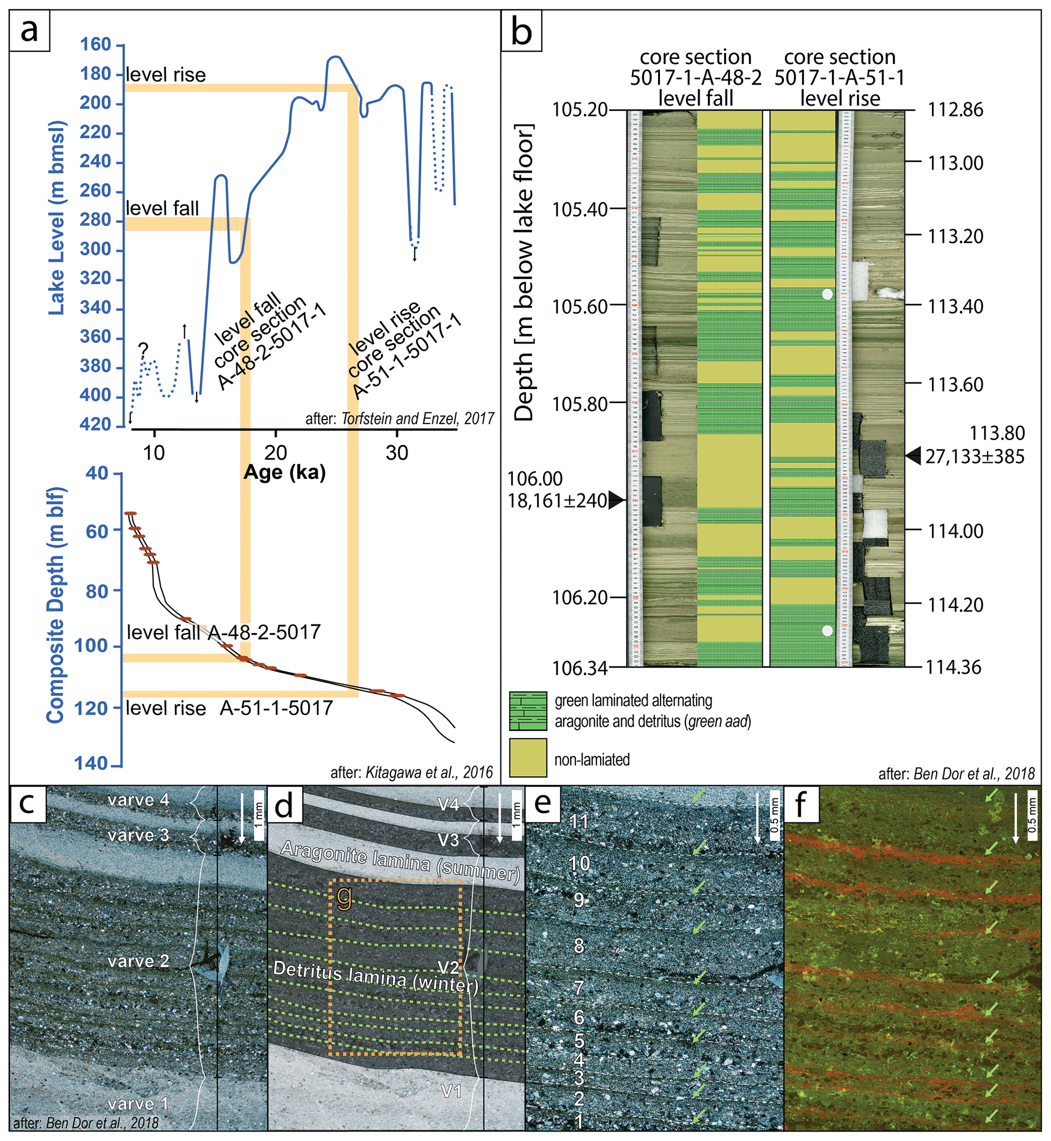
Figure 2(a) Top: Dead Sea lake level depicting the highest stage of Lake Lisan, the Late Pleistocene predecessor of the Dead Sea, during Last Glacial Maximum (Bartov et al., 2003; Torfstein and Enzel, 2017). Bottom: the age–depth model of the ICDP–DSDDP 5017-1 core and the position of the studied segments along the core (after Kitagawa et al., 2017). (b) The studied sections of the ICDP–DSDDP cores dated to 18 and 27 ka (marine isotope stage (MIS) 2, ∼ 15–30 ka). (c–f) Microscope images of alternating aragonite (summer precipitate) and detritus (deposited during winter) varves depicting a detrital lamina composed of multiple sub-laminae (labelled 1–11) deposited by individual floods (after Ben Dor et al., 2018).
3.1 Microfacies analyses
Two chronologically constrained segments (each ∼ 1.5 m long) of the ICDP–DSDDP 5017-1 core were selected for this study (Fig. 2; Neugebauer et al., 2014). These segments are coeval with opposing climatic trends, reflected by independently determined rising (27 ka) and falling (18 ka) lake-level trends (Bartov et al., 2002; Torfstein and Enzel, 2017). The two sections were sampled continuously with overlap to prepare a sequence comprising 10 cm long thin sections using a dry–freeze procedure adjusted for saline sediments (e.g., Brauer et al., 1999; Neugebauer et al., 2015) and analysed using a Hirox RH-2000 optical microscope (e.g., Ben Dor et al., 2018, 2021). A total of ∼ 700 varves (years) were counted and described in each segment. The segments comprise alternations of finely laminated varves (Ben Dor et al., 2019) and event-related deposits (ERDs; Neugebauer et al., 2014), attributed to debris flows (Ahlborn et al., 2018) and earthquakes (Fig. 2; Kagan et al., 2018). The nature of these sediments and their mode of formation, which is based on the study of available exposures (Begin et al., 1980, 1974; Stein et al., 1997; Marco et al., 1996) and modern analogous lakes (e.g., Dean et al., 2015; Roeser et al., 2021), suggest that these detritus–aragonite couplets were deposited annually, thus forming varves. This is further supported by the uniformity of the sediments revealed by microfacies analyses carried out in this study, in which slight changes in sediment properties are observed in detail, as well as by the agreement between laminae counting and independent radiometric dating using 14C and U–Th (Prasad et al., 2009; Haase-Schramm et al., 2004; Neugebauer et al., 2015). Because no deposition of alternating aragonite and detritus sedimentary facies takes place under modern conditions in the Dead Sea (e.g., Ben Dor et al., 2021), the interpretation of alternating aragonite and detritus facies as annual deposits is used within the framework of this study (e.g., Prasad et al., 2004; Ben Dor et al., 2019, 2020).
This study focuses on two properties of the varves that are interpreted as hydrological proxies: (a) the number of detrital sub-laminae in each detrital lamina, reflecting the number of flooding events that reached the coring site (Ben Dor et al., 2018), and (b) the thicknesses of aragonite laminae (this study). Because the thickness of detrital laminae (Fig. 2) is not directly linked to specific hydroclimatic processes but instead depends on the interaction of multiple factors such as sediment availability and the geographical position of the activated catchment, it is not analysed here as a hydroclimatic proxy. Because the typical number of sub-laminae is low and the minimal number of detrital sub-laminae that can be counted is 1, as no cases of “zero sub-laminae” are sedimentologically distinguishable, varves comprising a single detrital lamina are regarded as varves recording either years with no floods or years with a single flood. The two series deposited during rising and falling lake levels were compared using key statistical properties: the Mann–Whitney–Wilcoxon rank sum test to determine if they were sampled from two populations of a statistically different median (MWW; Mann and Whitney, 1947) and the Ansari–Bradley rank sum dispersion test (AB; Ansari and Bradley, 1960) to determine if their dispersions differ significantly. Missing data where laminae are trimmed or distorted (∼ 5 %) were imputed using singular spectrum analysis (e.g., Kondrashov and Ghil, 2006).
3.2 Detecting intra-record regime shifts
A non-parametric test was developed in order to identify regime shifts as part of this study, by comparing the observed running sum of the sub-lamina count normalized by its mean using consecutive multiple window widths ranging from 10 to 300 years, to surrogate series generated by point-wise permutations of the data (Eq. 1; Figs. 3 and S1–S5).
Equation (1) describes the normalized running sum of sub-lamina counts, where yw(i) is the normalized running sum, i is the location index ranging between 1 and N, N is the number of data points in the studied series, ∑nj is the sum of the sub-lamina count over the range between , w is the window width ranging from 10 to 300 by 10-year steps () , and is the mean normalized sum of n for window width w. Thus, yw(i) values larger than unity indicate flood-rich episodes, and yw(i) values lower than unity indicate flood-poor episodes.
Because the aim of this analysis is to assess the probability of observing decadal to centennial intervals of increased flood frequency (i.e., clustering of floods) whilst avoiding prior assumptions and parametrization and because the two series depict low serial dependence (Fig. S6), the surrogate time series were produced by point-wise permutations. After the running sum was normalized by its mean value for every window width, local maxima values that are separated by at least half of the window width were considered for the analysis (Fig. 3c and d). The peaks were ranked in descending order and compared to a dataset derived from 10 000 permutations without replacement of the respective series, revealing the significance level of observing flood-rich intervals of the studied window width. Observed values larger than the 95th percentile of the permutated series are considered statistically significant at the α=0.05 confidence level (Fig. 3e and f). Because the significant peaks of different window widths overlap, the clusters were evaluated by considering their summed probabilities (Fig. 3g and h), and their edges were refined using the running MWW and AB tests, in which the two halves of the window are compared to each other (Figs. S7–S8).
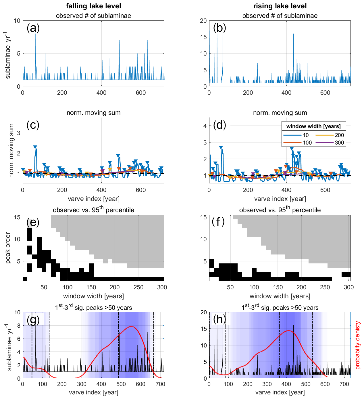
Figure 3Results of the non-parametric test developed for identifying flood-rich episodes (i.e., flood clustering). (a, b) The studied series of flood frequency analysed using microfacies analyses of two DSDDP core sections. (c, d) The running normalized sum calculated for identifying flood clusters and their peaks (triangle) using different window widths. (e, f) Binary diagrams indicating where observed yw(i) values are higher than the calculated 95th percentile of the distributions derived from 10 000 randomly permutated series and are thus statistically significant considering α=0.05 (black pixels) or non-significant (white pixels). Missing values, where not enough peaks were detected to calculate the 95th percentile, are coloured grey. (g, h) The location of statistically significant peaks at α=0.05 depicted as semi-transparent shading for the top three highly ranked peaks of window widths ranging between 50 and 300 superimposed on the data series. The red line depicts the probability of the summed identification of clusters by all window widths. The refined clusters are marked by dashed vertical lines.
Recurrence and joint-recurrence techniques and their analyses (RQA and JRQA) were applied to identify non-linear transitions and distinct regimes within the series (Eckmann et al., 1987). These methods can be used to detect abrupt transitions as well as short-term cyclic or oscillatory behaviours in non-stationary and noisy data by investigating their dynamics in the reconstructed phase space (Donges et al., 2011; Marwan et al., 2007). The following short introduction and the presented equations are based on the detailed review by Marwan et al. (2007), to which the keen reader is referred for further details.
The recurrence of the system is computed by considering the pairwise similarity (proximity) of points along its phase space trajectory, reconstructed using a selected time delay (τ) and an embedding dimension (m). The recurrence plot (RP), which is used to efficiently visualize the recurrence of the studied series, is plotted by calculating the Ri,j(ε) matrix through the binarization of the difference between the norm of the pairwise trajectories of steps in the reconstructed phase space using a predefined threshold ε (Eq. 2; Marwan et al., 2007). When the distance between two points along the trajectory (i and j) is smaller than ε, the value of the corresponding point (Ri,j(ε)) is set to unity in R and the pixel is painted black in the recurrence plot. Otherwise the value is set to zero and the corresponding pixel in the recurrence plot is painted white.
Equation (2) (after Marwan et al., 2007) describes the calculation of the recurrence matrix using a threshold ε, where N is the number of points of the reconstructed x trajectory and θ(⋅) is the Heaviside function (step function), where θ(x)=0 if x<0 and θ(x)=1 otherwise.
Similarly, the joint recurrence plot (JRP) can be derived for studying the dynamical relationship of two series or more as the product of their recurrence matrix (Eq. 3; Romano et al., 2004).
Equation (3) (after Marwan et al., 2007) describes the calculation of the joint recurrence matrix as the product of two recurrence matrices calculated for two series with trajectories x and y, using the thresholds εx and εy, respectively. N is the number of points of the trajectories, and θ(⋅) is the Heaviside function (step function), where θ(x)=0 if x<0 and θ(x)=1 otherwise.
The recurrence plot of a system characterized by cyclical components would show diagonal lines parallel to the line of identity (LOI), which connects its lower-left and upper-right corners, whereas a noisy system would be characterized by a spotty and random appearance of points throughout the recurrence plot. Once the recurrence plot is established, its properties and the time-dependent behaviour of the system can be studied by quantifying its recurrence using recurrence quantification analysis (RQA). This is done by computing different measures for each sub-matrix formed by sliding a square window along its LOI by a predefined time step. In this study the recurrence rate (RR), determinism (DET), the maximum length of a diagonal line within a sub-matrix (Lmax) and the laminarity (LAM) metrics are used. The maxima of DET and Lmax can be used to identify periodic–chaos and chaos–periodic transitions. Alongside those transitions, which are recorded as LAM minima, LAM could indicate chaos–chaos transitions as well (maxima). The recurrence rate is the percentage of points at which recurrence occurs within the studied segment (Eq. 4).
The determinism (DET) reflects the extent to which the system maintains an ordered, cyclic, and deterministic behaviour. Because uncorrelated, weakly correlated, stochastic, or chaotic processes form very short diagonal lines (if any), whereas deterministic processes generate longer diagonal lines, the ratio of recurrence points that form diagonal lines (with length ) to all recurrence points can be used to estimate the main behaviour of the system within the studied segment (Eq. 5). In this study the minimal length of l(lmin) was set to .
Similar to DET, LAM is computed as the portion of points forming vertical lines of minimal length v out of the entire set of recurrence points within the recurrence plot (or in its sub-matrices).
In order to decrease the influence of the tangential motion, LAM is computed using the points forming vertical lines (v) that exceed a minimal length (vmin), which was set in this study to . In cases where the recurrence plot consists of more single recurrence points than vertical structures, LAM will take low values.
Finally, the length of the longest diagonal line (Lmax) is computed by identifying the longest diagonal line found within the recurrence plot (or in its sub-matrices; Eq. 7).
where is the total number of diagonal lines.
This approach is specifically useful in this study because the studied proxies record the convolved non-linear interaction of climatic, hydrological, and limnogeological processes and because the effect of their interactions could stem from non-linear dynamics that have very different implications for sedimentary sections (Marwan and Kurths, 2004; Marwan et al., 2003). The analysis was carried out using the CRP toolbox for MATLAB© after normalizing the series to zero mean and unit standard deviation (ver. 5.22; Marwan et al., 2007). The embedding dimension and the time delay were determined using the false nearest-neighbour approach (Kennel et al., 1992) and the mutual-information method (Fig. S6; Marwan, 2011). The threshold ε was set to fit an RR of 0.1 using the max norm method (Schinkel et al., 2008), and the RQA (and JRQA) measures were calculated with a window of 30 years with a time step of a single year.
3.3 Analysis of oscillatory components
Hydrological data are commonly skewed and may exhibit short-term cyclic behaviour that is difficult to identify using standard Fourier-derived approaches such as the periodogram (e.g., Blackman and Tukey, 1958; Welch, 1967). Wavelet analyses provide a set of more flexible tools for identifying irregular and non-stationary cyclicities in short time series (Lau and Weng, 1995; Torrence and Compo, 1998). The coherence of two series provides an estimation of the importance of areas with high common power in the two series that reflect the localized correlation coefficient in time–frequency space (Grinsted et al., 2004). Wavelet analyses were carried out using the Morlet wavelet function after normalizing the data to zero mean and unit standard deviation. The significance of the wavelet power and coherence was determined against red noise simulated using a lag-1 autoregressive process (AR(1)) using the cumulative area-wise approach for detecting false positive periodicities at the alpha =0.05 confidence level (Schulte, 2019, 2016).
Singular spectrum analysis (SSA) is also used to identify periodic and oscillatory components in short, non-stationary, and noisy time series (Broomhead and King, 1986). Unlike wavelet and Fourier-based procedures, where the signal is compared to a predefined function, SSA identifies principal components that best explain the variance of the time-delayed series through the embedded matrix. This non-parametric approach reveals the dominant components that best explain the variance and defines their relative contribution to the observed signal (Vautard and Ghil, 1989). This, in turn, allows the breaking-down of the signal into its principal components and calculating their corresponding reconstructed components (RCs), which demonstrate the extent to which each component contributes to the signal (Ghil et al., 2002). Generally, SSA complements wavelet and other spectral analyses because it provides increased flexibility and may identify oscillatory components of different structures that change in time. Thus, the analyses of the individual RCs, and the determination of their dominant cyclical components can point to dominant frequencies embedded within the observed series, which in turn could stem from teleconnection patterns affecting hydroclimatic variability (e.g., NAO, SOI, etc.; e.g., Feliks et al., 2010; Le Mouël et al., 2019; Seager et al., 2019). In order to balance between the complexity and usefulness of the analyses, the SSA was performed with an embedding dimension (window) of 10 years after visually inspecting the effect of the number of RCs on the relevant eigenvalues. The first RC (RC(1)) was later used as the local trend component that was subtracted from the data as a high-pass filter to reveal short-term cyclicities (Fig. S9). The SSA RCs were additionally analysed using the Welch periodogram for evaluating the RC power spectral density (Welch, 1967) and wavelet analyses together with the area-wise significance test (Schulte, 2016, 2019) in order to compare their time–frequency properties during the identified cluster and background periods. The Welch periodogram was calculated after subtracting the mean from the series and zero-padding it to 211 points in order to minimize spectral leakage and applying a Hamming window of 25 years' width and an overlap of 50 %, in order to merge close periodic components and reduce spectral noise (Figs. S10–S13).
4.1 Microfacies analyses
The studied segments are dominated by greenish alternating laminae of aragonite and detritus (Fig. 2) and are characterized by a typical lamina thickness of < 1 mm. Detrital laminae are dominated by clay with quartz and organic matter, with some calcite, dolomite, and feldspar grains, commonly showing graded bedding, a clay cap, and a thin lamina of amorphous organic matter (Fig. 2). The laminated segments are interrupted by massive or graded-event-related deposits (ERDs) attributed to abrupt mass wasting events (e.g., turbidites and slumps), triggered by earthquakes (Kagan et al., 2018), debris flows, and slope instability (Ahlborn et al., 2018). Both lamina thickness and the number of sub-laminae show a statistically significant larger mean and variance during lake-level rise than during lake-level fall (Tables 1 and 2; Figs. 4 and 5).
Aragonite lamina thicknesses range between 51 and 2259 µm (μ=457 µm, σ=308 µm) and 53 and 6020 µm (μ=642 µm, σ=529 µm) during lake-level fall and rise, respectively. Detrital lamina thicknesses range from 27 to 13 136 µm (μ=312 µm σ=638 µm) and 27 and 8760 µm (μ=416 µm, σ=675 µm) in the falling and rising segments, respectively. The number of sub-laminae during the falling lake level ranges between 1 and 10 (μ=1.2, σ=0.7) and between 1 and 17 (μ=1.6, σ=1.6) during rising lake level (Table 1). The MWW test indicates a significant difference between all studied proxies when comparing the two studied series (p value ≪ 0.05). The difference in dispersions of all variables between rising and falling lake levels are statistically significant using the Ansari–Bradley test (p value ≪ 0.05) except for detrital laminae (p value ≈ 0.12; Table 2). All three parameters show positive skewness of 2.1 and 3.5 for aragonite lamina thickness, 12.7 and 7.6 for detrital aragonite laminae, and 5.9 and 6.1 of sub-lamina count during falling and rising lake levels, respectively. No significant correlation exists between any two of the parameters in each time series, with the exception of a moderate correlation between the number of sub-laminae in the detrital laminae and detrital lamina thickness (Fig. 5; r=0.30 and 0.49, for falling and rising lake levels, respectively; with p values ≪ 0.05).
Table 1Bulk statistical properties of the studied sedimentary series.
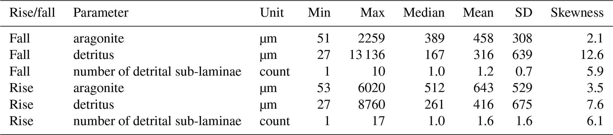
Table 2The p values of the statistical comparison between the bulk studied series.

1 MWW – Mann–Whitney–Wilcoxon rank sum test; AB – Ansari–Bradley dispersion test. 2 Tests with p values smaller than 0.05 are considered significant at α=0.05.
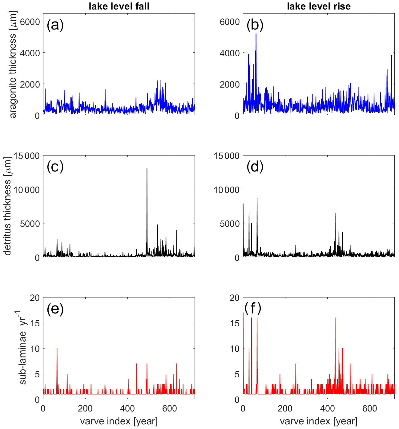
Figure 4Time series of microfacies analyses of the studied varved sections: (a, b; blue) aragonite lamina thickness, (c, d; black) detrital lamina thickness, (e, f; red) number of detrital sub-laminae.
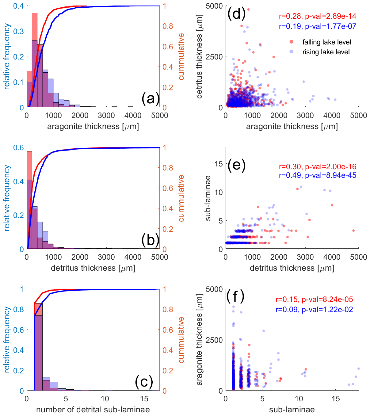
Figure 5Distributions and scatterplots of the trivariate geological time series showing the distributions of (a) aragonite lamina thickness, (b) detritus lamina thickness, and (c) number of sub-laminae counted in each detrital lamina. Plots (d)–(f) show the correlations between aragonite and detritus thickness (d, r2=0.08, 0.04), number of floods and detritus thickness (e, r2=0.09, 0.24), and number of floods and aragonite lamina thickness (f, r2=0.02, 0.01).
4.2 Detecting intra-record regime shifts
Two clusters of intense flood frequency were identified in each of the studied series (Fig. 3; Table 3). However one of the two clusters in each series appears more robust in comparison with the other, as it was identified using multiple window widths (Fig. S5), and the clusters are labelled as robust and less robust accordingly (Table 3). However, it is noted that this different robustness estimation could stem from an “edge effect” bias, which limits the analysis of segments close to the edges of the series when large window widths are applied. The recurrence plots of aragonite series depict some short diagonal lines, whereas those of the sub-laminae show more spotty properties with a blocky character (Figs. 6 and 7). An increase in both DET and Lmax is identified close to edges of clusters, although the RQA measures fluctuate throughout the series and do not exhibit pronounced changes or trends with respect to the identified clusters. Both JRPs depict fairly low recurrence with spotty and patchy patterns, with some diagonal lines in the series of the falling lake level.
Table 3Identified clusters in the two studied series following the procedure described in Sect. 3.2 using the number of detrital sub-laminae.
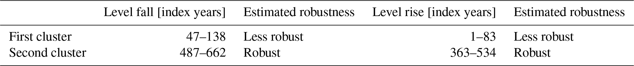
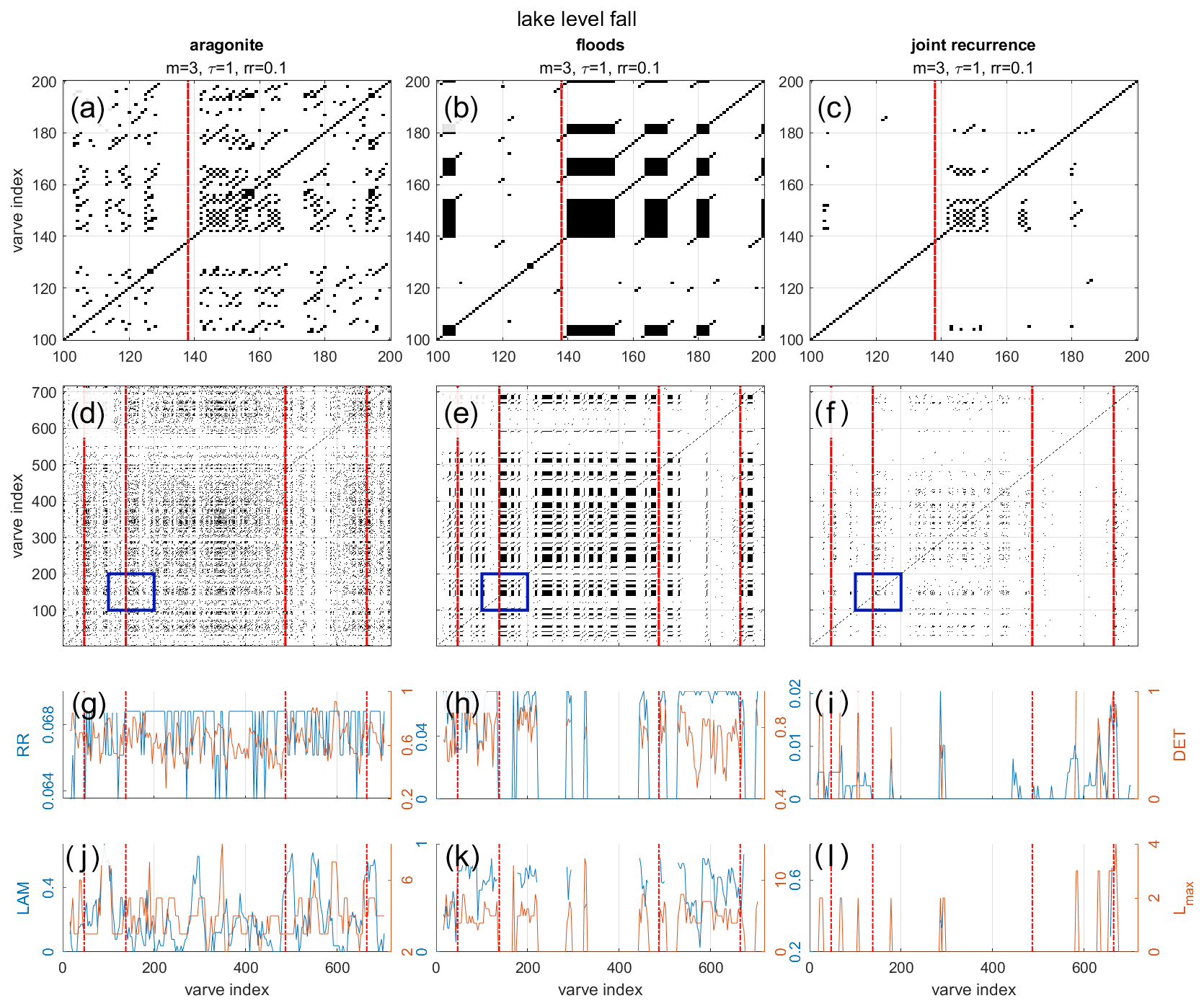
Figure 6(a–c) Enlarged segments of the recurrence plots of the studied lake-level fall for aragonite thickness (a), flood frequency (b), and the joint recurrence plot for the two proxies (c). (d–f) Recurrence plots of the aragonite thickness (d) and flood frequency (e) and the joint recurrence plot for the two proxies (f), with blue rectangles indicating the extent of data presented in (a)–(c). Note the parallel diagonal lines that characterize series of the aragonite thickness (a, d) and point to an inherent oscillatory behaviour, whereas the flood series (b, e) forms sporadic points and polygons that reflect a more chaotic or random behaviour. (g–i) The recurrence rate (RR) and the determinism (DET) coefficient calculated using a running window size of 30 years and a single-year step for aragonite thickness (g), floods (h), and their joint recurrence (i). (j–l) The laminarity (LAM) and the maximum length of the diagonal line within the sub-matrix (Lmax) coefficient using a running window size of 30 years and a single-year step for aragonite thickness (j), floods (k), and their joint recurrence (l). The analyses were performed after detrending the data by subtracting the RC(1) of the SSA and normalizing to zero mean and unit standard deviation. The selected parameters for the embedding are m (dimension), τ (delay), and ε (threshold) used for space phase reconstructions and depicted in the figure. Red lines represent possible clusters identified independently of the recurrence analyses.

Figure 7(a–c) Enlarged segments of the recurrence plots of the studied lake-level rise for aragonite thickness (a), flood frequency (b), and the joint recurrence plot for the two proxies (c). (d–f) Recurrence plots of the aragonite thickness (d) and flood frequency (e) and the joint recurrence plot for the two proxies (f), with blue rectangles indicating the extent of data presented in (a)–(c). Note the parallel diagonal lines that characterize the series of aragonite thickness (a, d) and point to an inherent oscillatory behaviour, whereas the flood series (b, e) forms sporadic points and polygons that reflect a more chaotic or random behaviour. (g–i) The recurrence rate (RR) and the determinism (DET) coefficient calculated using a running window size of 30 years and a single-year step for aragonite thickness (g), floods (h), and their joint recurrence (i). (j–l) The laminarity (LAM) and the maximum length of the diagonal line within the sub-matrix (Lmax) coefficient using a running window size of 30 years and a single-year step for aragonite thickness (j), floods (k), and their joint recurrence (l). The analyses were performed after detrending the data by subtracting the RC(1) of the SSA and normalizing to zero mean and unit standard deviation. The selected parameters for the embedding are m (dimension), τ (delay) and ε (threshold) used for space phase reconstructions and depicted in the figure. Red lines represent possible clusters identified independently of the recurrence analyses.
4.3 Analysis of oscillatory components
The appearance of short diagonal lines in the recurrence plot of the aragonite thickness series indicates either intermittent periodic or weakly to moderately chaotic behaviours (Figs. 6 and 7). Conversely, the flood frequency series present blocky and irregular patterns that indicate an underlying chaotic, random, or practically non-periodic process (Figs. 6 and 7). In particular, the segments identified as clusters demonstrate some abrupt changes in the studied RQA measures that could indicate a shift in the systems' dynamics, both in aragonite thickness and in the number of sub-laminae. Although this behaviour is somewhat expected for the sub-lamina series that was used to determine clusters in the first place, it is also evident for the aragonite series.
Discontinuous short-term patches of increased spectral power at annual–decadal timescales appear sporadically throughout the entire dataset in both aragonite and flood frequency series (Fig. 8). However, these short-term periodic components are not significant at an α = 0.05 confidence level and do not pass the global significance test. Instead, a couple of the significant patches that appear within this spectral band appear within clusters as vertical patches that stretch over a range of timescales from sub-decadal to a multi-decadal (30–60 years) frequency bands, which indicate that the elevated spectral power in those frequency bands can be attributed to the abrupt pulse of increased variance occurring during the identified clusters (e.g., Hochman et al., 2019). Nevertheless, several of these significant patches pass the global significance test after detrending using the RC(1) of the SSA (Fig. S14). High spectral power in the centennial to bicentennial band (∼ 120–250 years) is observed in both series of aragonite thicknesses, although its significance cannot be determined as it falls largely outside the cone of influence, and it fails the cumulative area-wise significance test. A similar cyclical component is also identified in the sub-lamina series during lake-level rise but not in the interval of lake-level fall. Altogether, the wavelet analyses do not suggest a robust detection of cyclical components in any of the studied series.

Figure 8Wavelet and global wavelet spectrograms of aragonite thickness and flood frequency during falling (left) and rising (right) episodes. Patches with significance level above 0.95 (α=0.05) detected using the cumulative area-wise significance test are depicted by a bold black line (Schulte et al., 2018; Schulte, 2016). Each triplot section shows the normalized data (a–d), the wavelet spectrograms (e–h), and the global wavelet spectra (blue) compared to the significance level of the global wavelet power spectra (dashed black, i–l). Significant peaks are marked in red (Schulte, 2019). Dashed vertical lines in (e)–(h) depict clusters identified as episodes of increased flood frequency. Note that the short-term cyclical components in the global wavelet spectra, which fail the significance test using the original series, are found to be significant in the analysis of the detrended series (Fig. S14).
The SSA RCs are characterized by several cyclical components (Figs. S10–S13). The first two components are regarded as the local trend component and accordingly depict persistent “long-wave” cyclical components characterized by a timescale of > 32 years. The other components roughly show three peaks characterized by cyclical components of sub-decadal frequencies.
5.1 The mechanistic link between mean properties and variability
The poor correlation between aragonite thickness and the number of sub-laminae testifies to their low inter-dependence and strengthens their interpretation as (nearly) independent proxies of the hydrological cycle in the Dead Sea watershed, which is in accordance with the previous interpretation of their relationship with the hydrological cycle (Ben Dor et al., 2018, 2021). Because of the unique hydroclimatic settings of the lake and its sedimentary record, it cannot be directly interpreted using a standard flood frequency analysis (e.g., Metzger et al., 2020), where the frequency and magnitude of floods in individual watersheds are studied. Indeed, the detrital sub-laminae in the ICDP–DSDDP core capture the number of flooding events, potentially lasting up to several days (Nehorai et al., 2013), which exceeded the threshold required to reach the coring site at the lake depocenter (Ben Dor et al., 2018), instead of recording discharge properties at individual watersheds. Furthermore, the bathymetry of the basin dictates that only large enough floods in tributaries situated on both escarpments in front of the coring site could have deposited detrital material at the coring site (Fig. 1). Although this aspect masks some of the delicate features that could have been otherwise extracted, such as in the analyses of modern measurements, its length and established context with respect to regional climatic conditions demonstrates its value for interpreting hydroclimatic variability during episodes of climate change.
Available modern observations of sediment and water transport paths into the lake cannot unambiguously determine which synoptic systems affected the eastern Mediterranean Sea when the studied sediment segments were deposited during the Last Glacial Maximum (LGM). Nevertheless, considering available data that address this question, the likely suggestion that dominant weather regimes and synoptic circulation patterns during the LGM were similar to the present is adopted for the sake of discussion in the framework of this work (e.g., Greenbaum et al., 2006; Amit et al., 2011; Enzel et al., 2008) while considering possible modifications of their spatial properties (e.g., Goldsmith et al., 2017; Keinan et al., 2019). By considering that the dominant synoptic-scale circulation patterns during the Late Pleistocene resemble modern observations in the region (Enzel et al., 2008), it can be argued that flooding, recorded as detrital sub-laminae at the depocenter of Lake Lisan, can be attributed to any of the three key synoptic patterns that govern precipitation over the eastern Mediterranean Sea and southern Levant (e.g., Armon et al., 2019). It is further suggested that the interplay and relative frequency of these three systems determine mean climatic conditions, which, in turn, determines the Dead Sea lake level and ultimately propagates into its sedimentary record (Torfstein et al., 2015; Neugebauer et al., 2014). Thus, the association of increased flood frequency with rising lake levels was interpreted as reflecting increased frequency and/or modulation of the Mediterranean Low characteristics that deliver the majority of annual precipitation to the Dead Sea watershed and hence determine annual inflow into the lake (Saaroni et al., 2010; Enzel et al., 2008; Armon et al., 2019). However, a more detailed comparison of flood frequency with aragonite lamina thickness that reflects annual inflow into the lake and the dilution of its epilimnion (Kolodny et al., 2005; Stein et al., 1997; Ben Dor et al., 2021) reveals more subtle insights and a delicate interplay of hydroclimatic factors manifested through the watershed during opposing climatic regimes.
Both aragonite lamina thickness and flood frequency have larger mean and variance during lake-level rise (Table 1). Because rising lake levels indicate a wetter climate on average, this relationship between mean and variance is similar to that observed in modern hydrologic phenomena such as precipitation (e.g., Morin et al., 2019). The observed relationship between the two studied properties thus strengthens the interpretation of these sedimentary proxies as hydroclimatic proxies. Namely, the increased thickness of aragonite laminae and the increased number of detrital sub-laminae suggests that the episodes of rising lake level were characterized by both increased annual inflow and increased flood frequency. The ongoing debate on the effects of climate change on flood frequency resulted in approaches suggesting that increased frequency of floods is coupled with drying of the eastern Mediterranean or with wetter climatic conditions (e.g., Alpert et al., 2002; Rohling, 2013; Yosef et al., 2019). The results presented here suggest that increased flood frequency is likely coupled with wetter intervals rather than with dryer conditions in the eastern Mediterranean. Furthermore, the observed coupling of increased thickness of aragonite laminae with increased flood frequency may support their formation by a common hydroclimatic mechanism, i.e., the increased occurrence of Mediterranean Lows (Armon et al., 2019; Enzel et al., 2008; Ben Dor et al., 2018; Goldreich et al., 2004).
5.2 Oscillatory components and hydroclimatological pacing
One of the goals in studying hydroclimatological proxies is identifying key cyclical components that pace short-term variability under different mean climatic regimes (e.g., Ghil et al., 2002; Grinsted et al., 2004). Because (a) the thickness of aragonite laminae was suggested to reflect hydroclimatic (Kolodny et al., 2005) and limnologic conditions (Ben Dor et al., 2021) and (b) cyclical behaviour attributed to solar cycles was previously identified by spectral analyses of lamina thickness at the exposed coeval White Cliff Member of the Lisan Formation at Masada deposited during MIS2 (Prasad et al., 2004), a similar attempt was made in this study to identify cyclical components as well. Although Prasad et al. (2004) reported cyclical components of 50–60 years, the increased power observed in these spectral bands was not found to be significant in the studied sections at the α=0.05 confidence level (Fig. 8; Schulte, 2016, 2019).
The North Atlantic Oscillation (NAO) and the eastern Atlantic (EA) patterns were suggested to affect inter-annual precipitation variability over the eastern Mediterranean Sea (e.g., Feldstein and Dayan, 2008; Feliks et al., 2010; Krichak et al., 2002; Seager et al., 2019), primarily due to their reported effect on discrete precipitation-bearing synoptic patterns over the eastern Mediterranean (e.g., Black, 2012). Other studies, on the other hand, have suggested that unlike in western Turkey, NAO shows only minimal direct impact on precipitation in the Levant and that it might affect temperature instead (Enzel et al., 2003; Seager et al., 2020; Ziv et al., 2006). Although such relationships are hard to identify in geological records, a North Atlantic impact over the Dead Sea hydrology during the last glacial was identified by lake-level reconstructions, where abrupt lake-level drops took place during Heinrich events (Bartov et al., 2003). Additionally, a cyclical component of sub-decadal to decadal frequency bands (4–5, 7–8, and ∼ 11 years), which were attributed to NAO, was also identified in laminated halite sequences deposited during the last interglacial (Palchan et al., 2017). These authors interpreted the cyclicity based on modern observations, which indicate that such pacing may manifest temperature variations rather than precipitation, as temperature seasonality controls halite deposition rather than hydrologic forcing (Sirota et al., 2017, 2018).
Additionally, previously reported δ18O and δ13C from ∼ 200 aragonite laminae recovered from MIS2 exposures of the Lisan Formation at Masada and Perazim Valley were analysed using wavelet analyses. Because the systematics of these isotopic compositions are distinctly different, these proxies have different implications for environmental conditions in the lake and its surroundings. More specifically, δ18O is directly influenced by hydroclimatology, whereas δ13C is primarily affected by biological activity (Kolodny et al., 2005). Nevertheless, it appears that because the extent of biological activity in Lake Lisan depended on freshwater inflow that also replenished its surface water with required nutrients (Begin et al., 2004), the two proxies share similar pacing and are broadly characterized by a non-persistent band of cyclicities of annual to decadal timescales that fail the cumulative area-wise significance test at the α=0.05 level, although the coherence of this band between the signals is significant and shows a similar phase relationship (Fig. 9).
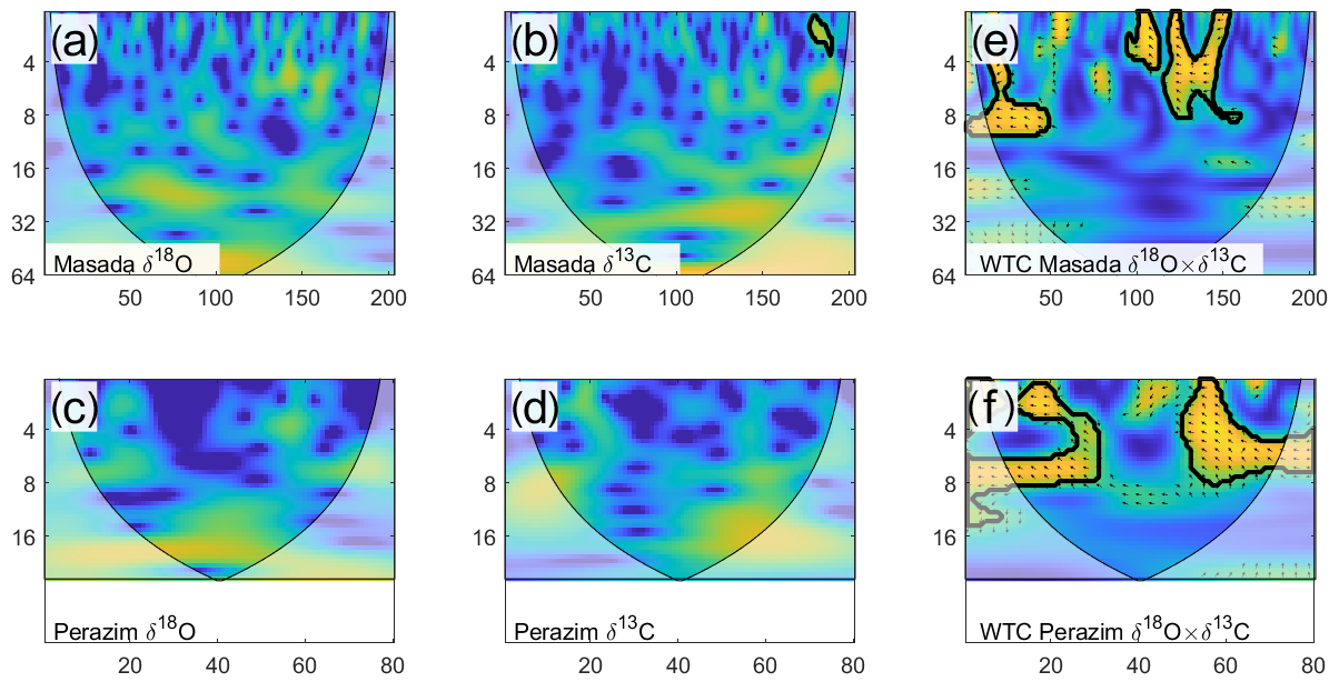
Figure 9Wavelet (a–d) and wavelet coherence (e–f) analyses of δ18O and δ13C in two segments of the Masada (30 ka) and Perazim (25 ka) exposures of the White Cliff Member (Lisan Formation) deposited during the last glacial over the shelf of Lake Lisan. Areas with significance level above 0.95 (α=0.05) are marked by a thick black line. Data are from Kolodny et al. (2005).
Century-long precipitation data from the Kfar Giladi and Jerusalem stations correlate well with pre-regulated modern Dead Sea levels and are thus considered to reflect mean hydrological conditions over the northern and central parts of the Dead Sea watershed in recent and past times (Enzel et al., 2003; Morin et al., 2019). Thus, available precipitation records at both stations were also compared to the winter (DJF) NAO and EA indices using wavelet and wavelet coherence in order to detect common pacing and cyclical components (Figs. S15 and S16; NOAA, 2020). These relatively short records do not exhibit significant cyclical components and no significant coherence either. However, although the available records do not exhibit significant cyclical behaviour (at α=0.05), increased non-significant spectral power of short-term fluctuations is evident in the ICDP–DSDDP cores (Figs. 8, S6, S10-S13), in the isotopic composition of aragonite laminae (Fig. 9; Kolodny et al., 2005), in modern precipitation records, and in the winter indices of teleconnection patterns (Figs. S15 and S16). This statistically non-significant similarity, could either point to the lack of influence of NAO and EA on hydroclimate or to a weak and non-linear effect of these teleconnection patterns on precipitation in the eastern Mediterranean (Black, 2012). Alternatively, this can point to the inherent difficulties in detecting such delicate relationships from sedimentary archives that ultimately record the interaction of complex hydrological and limnological processes involved in lamina formation and post-depositional changes, such as the non-homogenous spread of fine-grained sediments over the lake floor and the effects of inflows from different catchments.
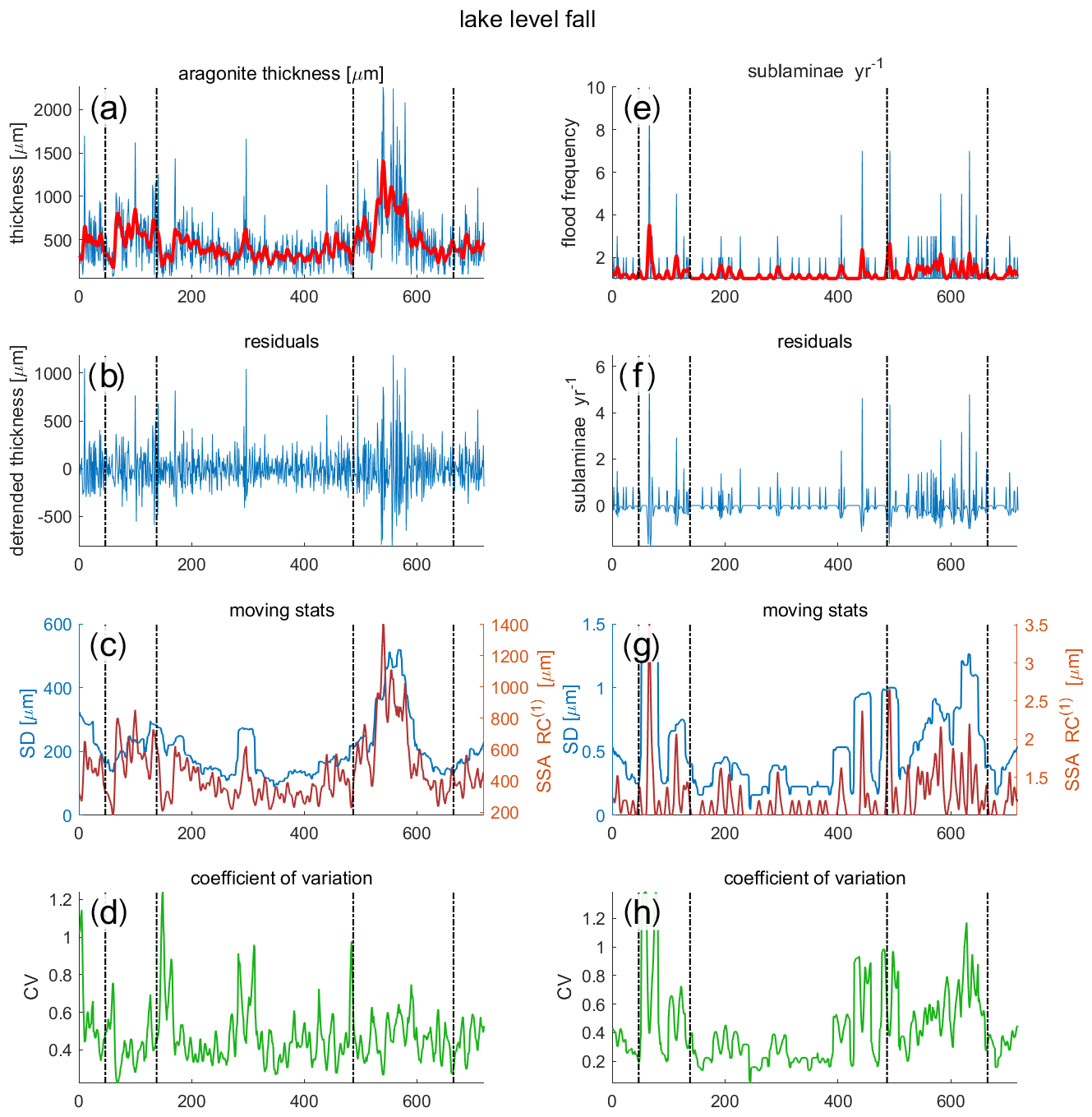
Figure 10Running statistical properties of aragonite lamina thickness (a–d) and flood frequency (e–h) for the studied lake-level fall. The measured data (a, e), the residuals (after subtracting the RC(1)) (b, f), RC(1) and running standard deviation (30-year window) (c, g), and the coefficient of variation calculated as (d, h).
5.3 Clusters and regime transitions
The studied episodes demonstrate pronounced centennial-scale clustering of flooding events (Fig. 3). Similarly, other high-resolution palaeo-hydrological records (e.g., Witt et al., 2017) and modern observations (e.g., Metzger et al., 2020) have demonstrated non-uniform and non-Poissonian flood frequencies. In addition, the clusters observed during lake-level fall are characterized by flood frequencies similar to those appearing in the background episodes during lake-level rise (Figs. S17 and S18). This suggests that the wetter episodes are characterized by increased mean precipitation and variability as well as by increased frequency of intense storms, which is in agreement with modern observations (Morin et al., 2019).
The comparison of aragonite lamina thickness of the two clusters identified in each of the studied intervals reveals opposing properties, which become evident by comparing their RC(1) and dispersion, which is calculated as the running standard deviation of the residuals (after subtracting RC(1); Figs. 10 and 11). In each of the studied intervals, one cluster demonstrates increased mean and variance in both flood frequency and aragonite thickness, whereas the other cluster is characterized by increased mean flood frequency but the thickness of its aragonite laminae is characterized by the mean and dispersion that are similar to that of background episodes (Figs. S17 and S18). In order to address these observations, a unified explanation that can account for this discrepancy is hereby suggested by considering the modern hydroclimatic regime and dominant synoptic circulation patterns.
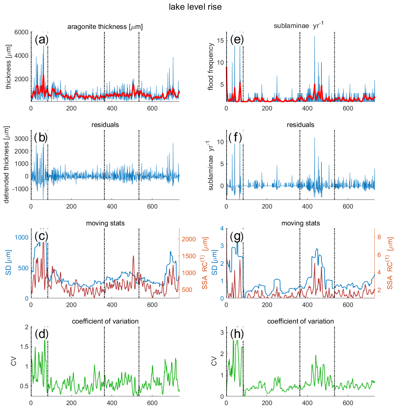
Figure 11Running statistical properties of aragonite lamina thickness (a–d) and flood frequency (e–h) for the studied lake-level rise. The measured data (a, e), the residuals (after subtracting the RC(1)) (b, f), RC(1) and running standard deviation (30-year window) (c, g), and the coefficient of variation calculated as (d, h).
Although modern records are relatively short and the comparison of sparse hydrological measurements with the detailed framework of atmospheric circulation only permits cautious suggestions at this stage, the above-mentioned observations can be explained using the modern synoptic framework by considering two distinct synoptic and hydroclimatic scenarios that govern flood generation and their clustering over the catchments that face the ICDP–DSDDP coring site. Most of the precipitation over the Dead Sea watershed is delivered by Mediterranean Lows during the winter months (e.g., Enzel et al., 2003; Saaroni et al., 2010; Ziv et al., 2006). When these cyclones are deep and are characterized by a southern track, their resulting precipitating clouds can have a pronounced impact on the Dead Sea watershed and generate more rainfall and therefore effectively deliver more precipitation to the watershed (Ziv et al., 2006; Saaroni et al., 2010). Thus, under these conditions they increase annual precipitation and the chances of generating floods over the catchments that face the ICDP–DSDDP coring site (e.g., Armon et al., 2019; Belachsen et al., 2017; Goldreich, 2004). As suggested above, this scenario could account for the observed coupled increase in both mean and variance of flood frequency and aragonite lamina thickness, observed in one of the clusters in each of the studied series (Figs. S17 and S18).
The general understanding of precipitation patterns induced by different synoptic systems in the Dead Sea watershed depicts a “de-coupling” of annual inflow into the lake, which depends on annual precipitation over the northern parts of the watershed, and floods reaching the coring site. This is because the frequency and intensity of Mediterranean Lows determines annual precipitation over the watershed (Saaroni et al., 2010) and flood frequency in the relevant ephemeral streams (Goldreich et al., 2004), whereas the contribution of the other synoptic systems to annual precipitation is, by far, less substantial (Armon et al., 2019; Marra et al., 2021). This is also evident by the low correlation (r2=0.086) of major floods (defined as flood peaks with a return period > 5 years) in the Negev Desert (Kahana et al., 2002) and precipitation in Jerusalem, which is closely correlated with Dead Sea lake level and hence with annual inflow into the lake (Enzel et al., 2003). Thus, although this cannot be directly proven for the LGM, these modern observations are considered here as means for deciphering the sedimentary record (e.g., Enzel et al., 2008; Goldsmith et al., 2017).
During the other cluster, on the other hand, the observed increased flood frequency is not coupled with increased mean and variance of aragonite lamina thickness. Studies of modern floods and their synoptic settings indicate that floods over the eastern Mediterranean are also generated by two additional synoptic systems: the active Red Sea trough (ARST) and disturbances to the subtropical jet stream (or tropical plumes). These synoptic conditions can generate significant floods over the small catchments surrounding the ICDP–DSDDP coring site, thus having the potential to deliver sediments but, owing to their spatiotemporal properties and frequency, providing a negligible contribution to annual inflow into the lake (Armon et al., 2019). Under current conditions, ARSTs are more frequent than tropical plumes and are characterized by high peak discharge and floods of relatively low volume (e.g., Armon et al., 2018; Shentsis et al., 2012). The second cluster may be therefore explained by increased frequency of ARSTs during decades of decreased mean annual precipitation. This scenario would result in increased flood frequency, recorded by more sub-laminae, without substantially increasing annual inflow, thus exhibiting aragonite thicknesses similar to background periods.
The short-term hydroclimatic variability of opposing climatic trends in the Levant was studied in detail through several analyses of two annually resolved varve sequences of the ICDP–DSDDP cores, representing opposing mean climates recorded by contrasting lake-level trends. This unique sedimentary record complements the otherwise short and sparse modern climatic and hydrological records and elucidates aspects and properties of regional hydroclimatology on a centennial timescale. By the analyses of two sedimentary proxies that reflect annual inflow and flood frequency and by their comparison with modern climatic data and synoptic observations, new insights on hydroclimatic stationarity during Late Pleistocene climate changes were revealed. These findings improve our understanding of short-term Late Pleistocene hydroclimatic variability.
Key conclusions arise:
-
The variance of both aragonite lamina thickness and flood frequency in the ICDP–DSDDP cores changes with their mean, as observed in modern hydrologic records. These findings strengthen the interpretation of these proxies as recorders of hydroclimatic phenomena in the Dead Sea watershed. During the wetter interval, which is characterized by lake-level rise, both the mean and the variance of these proxies are larger than during the studied episode of falling lake level.
-
No significant cyclical components were identified in the studied records using singular spectrum, wavelet, and recurrence analyses. However, it is suggested that this could stem from the interaction of climatic, hydrologic, and limnogeological processes that may have reduced the signal-to-noise ratio of the studied proxies. Nevertheless, the integration of these methods suggests that some short-term oscillatory components could have affected annual precipitation and flood frequency during the Late Pleistocene but were not found to be significant in the studied sedimentary sections.
-
Flood frequencies demonstrate hydroclimatic regime shifts operating at the centennial timescale. Floods are clustered into episodes that depict two distinct relationships between the mean and the dispersion of flood frequency and annual inflow. Namely, in each studied series one cluster is characterized by increased mean and variance of the two proxies, whereas the other cluster is characterized by increased mean and dispersion of flood frequency, which is not observed in annual precipitation. This implies that one of the clusters was generated by a distinct hydroclimatic regime that was characterized by a different dominance of synoptic circulation patterns, which resulted in increased flood frequency at the decadal scale but without increasing annual precipitation. Thus, it may suggest that clusters of increased flood frequencies could result either from an increased frequency of Mediterranean Lows or of active Red Sea troughs. Such regime shifts could also affect modern and future conditions that would manifest as drastic hydroclimatic shifts at decadal to centennial scales.
The code utilized for this research are available upon request from the corresponding author. Some of the analyses utilize available scripts and packages for wavelet analyses (Schulte, 2019, 2016; Grinsted et al., 2004; Torrence and Compo, 1998; Schulte et al., 2018), SSA (e.g., https://dept.atmos.ucla.edu/tcd/ssa-tutorial-matlab, Groth, 2016), and recurrence plots and their analyses (Marwan, 2016; Marwan et al., 2007) using MATLAB.
The data used for this research is available upon request from the corresponding author.
The supplement related to this article is available online at: https://doi.org/10.5194/cp-17-2653-2021-supplement.
YE, EM, and AB conceptualized the research and obtained the funding to support it. EM, MA, FM, and YBD performed statistical analyses, provided the context of relevant modern hydrometeorological phenomena for interpreting the data, and wrote the parts addressing hydroclimatological phenomena and climate. AB, MJS, YE, and YBD provided the geomorphological and limnological context for interpreting the findings and wrote the parts related to core acquisition, sedimentary microfacies analyses and their interpretation. AB and MJS provided guiding and laboratory support for microfacies analyses and their interpretation. MJS and YBD sampled the cores and aided in thin-section preparation. YBD performed microfacies and statistical analyses and wrote the paper with input from all authors. All authors reviewed the paper and provided their input during writing and revision.
The contact author has declared that neither they nor their co-authors have any competing interests.
Publisher's note: Copernicus Publications remains neutral with regard to jurisdictional claims in published maps and institutional affiliations.
This study is a contribution to the PALEX project “Paleohydrology and Extreme Floods from the Dead Sea ICDP core”. The authors acknowledge the support and contribution of laboratory staff and technicians at the GFZ, where preparation of thin sections and photography were carried out. We thank Jens Mingram, Norbert Nowaczyk, Brian Brademann, Florian Ott, Nadine Dräger, and Matthias Köppel for technical support and fruitful discussions. We are grateful for the comments made by Reik Donner, two anonymous reviewers, and the handling editor Pierre Francus during the review process, which altogether have helped to substantially improve the paper.
This research has been supported by the Deutsche Forschungsgemeinschaft (grant no. BR2208/13-1/-2) to Achim Brauer, Yehouda Enzel, Efrat Morin, and Yigal Erel and the Israel Science Foundation (grant no. 1436/14). Yoav Ben Dor was funded by a scholarship from the Advanced School of Environmental Studies, the Hebrew University of Jerusalem, and by the Rieger Foundation-Jewish National Fund programme for environmental studies as well as the Pfeifer grant for postdoctoral fellows at the Institute of Earth Sciences at the Hebrew University of Jerusalem.
This paper was edited by Pierre Francus and reviewed by Reik Donner and two anonymous referees.
Ahlborn, M., Armon, M., Ben Dor, Y., Neugebauer, I., Schwab, M. J., Tjallingii, R., Shoqeir, J. H., Morin, E., Enzel, Y., and Brauer, A.: Increased frequency of torrential rainstorms during a regional late Holocene eastern Mediterranean drought, Quaternary Res., 89, 425–431, https://doi.org/10.1017/qua.2018.9, 2018.
Allen, K., Hope, P., Lam, D., Brown, J., and Wasson, R.: Improving Australia's flood record for planning purposes – can we do better?, Australasian Journal of Water Resources, 24, 36–45, 2020.
Alpert, P., Ben-Gai, T., Baharad, A., Benjamini, Y., Yekutieli, D., Colacino, M., Diodato, L., Ramis, C., Homar, V., Romero, R., Michaelides, S., and Manes, A.: The paradoxical increase of Mediterranean extreme daily rainfall in spite of decrease in total values, Geophys. Res. Lett., 29, 31-31–31-34, https://doi.org/10.1029/2001GL013554, 2002.
Amit, R., Simhai, O., Ayalon, A., Enzel, Y., Matmon, A., Crouvi, O., Porat, N., and McDonald, E.: Transition from arid to hyper-arid environment in the southern Levant deserts as recorded by early Pleistocene cummulic Aridisols, Quaternary Sci. Rev., 30, 312–323, 2011.
Ansari, A. R. and Bradley, R. A.: Rank-sum tests for dispersions, Ann. Math. Stat., 31, 1174–1189, 1960.
Armon, M., Dente, E., Smith, J. A., Enzel, Y., and Morin, E.: Synoptic-Scale Control over Modern Rainfall and Flood Patterns in the Levant Drylands with Implications for Past Climates, J. Hydrometeorol., 19, 1077–1096, https://doi.org/10.1175/jhm-d-18-0013.1, 2018.
Armon, M., morin, E., and Enzel, Y.: Overview of modern atmospheric patterns controlling rainfall and floods into the Dead Sea: Implications for the lake's sedimentology and paleohydrology, Quaternary Sci. Rev., 216, 58–73, 2019.
Armon, M., Marra, F., Enzel, Y., Rostkier-Edelstein, D., and Morin, E.: Radar-based characterisation of heavy precipitation in the eastern Mediterranean and its representation in a convection-permitting model, Hydrol. Earth Syst. Sci., 24, 1227–1249, https://doi.org/10.5194/hess-24-1227-2020, 2020.
Avni, S., Joseph-Hai, N., Haviv, I., Matmon, A., Benedetti, L., and Team, A.: Patterns and rates of 103–105 yr denudation in carbonate terrains under subhumid to subalpine climatic gradient, Mount Hermon, Israel, GSA Bull., 131, 899–912, 2018.
Baker, V. R.: Paleoflood hydrology: Origin, progress, prospects, Geomorphology, 101, 1–13, 2008.
Bar-Matthews, M., Ayalon, A., Kaufman, A., and Wasserburg, G. J.: The Eastern Mediterranean paleoclimate as a reflection of regional events: Soreq cave, Israel, Earth Planet. Sc. Lett., 166, 85–95, 1999.
Bar-Matthews, M., Ayalon, A., Gilmour, M., Matthews, A., and Hawkesworth, C. J.: Sea–land oxygen isotopic relationships from planktonic foraminifera and speleothems in the Eastern Mediterranean region and their implication for paleorainfall during interglacial intervals, Geochim. Cosmochim. Ac., 67, 3181–3199, 2003.
Bartov, Y., Stein, M., Enzel, Y., Agnon, A., and Reches, Z.: Lake levels and sequence stratigraphy of Lake Lisan, the Late Pleistocene precursor of the Dead Sea, Quaternary Res., 57, 9–21, 2002.
Bartov, Y., Goldstein, S. L., Stein, M., and Enzel, Y.: Catastrophic arid episodes in the Eastern Mediterranean linked with the North Atlantic Heinrich events, Geology, 31, 439–442, 2003.
Bartov, Y., Enzel, Y., Porat, N., and Stein, M.: Evolution of the Late Pleistocene–Holocene Dead Sea Basin from sequence statigraphy of fan deltas and lake-level reconstruction, J. Sediment. Res., 77, 680–692, 2007.
Begin, Z., Ehrlich, A., and Nathan, Y.: Lake Lisan, the Pleistocene precursor of the Dead Sea. Israel Geological Survey, Bulletin 63, 30 pp., 1974.
Begin, Z. B., Nathan, Y., and Ehrlich, A.: Stratigraphy and facies distribution in the Lisan Formation – new evidence from the area south of the Dead Sea, Israel, Israel J. Earth Sci., 29, 182–189, 1980.
Begin, Z. B., Stein, M., Katz, A., Machlus, M., Rosenfeld, A., Buchbinder, B., and Bartov, Y.: Southward migration of rain tracks during the last glacial, revealed by salinity gradient in Lake Lisan (Dead Sea rift), Quaternary Sci. Rev., 23, 1627–1636, https://doi.org/10.1016/j.quascirev.2004.01.002, 2004.
Belachsen, I., Marra, F., Peleg, N., and Morin, E.: Convective rainfall in a dry climate: relations with synoptic systems and flash-flood generation in the Dead Sea region, Hydrol. Earth Syst. Sci., 21, 5165–5180, https://doi.org/10.5194/hess-21-5165-2017, 2017.
Belmaker, R., Lazar, B., Stein, M., Taha, N., and Bookman, R.: Constraints on aragonite precipitation in the Dead Sea from geochemical measurements of flood plumes, Quaternary Sci. Rev., 221, 105876, https://doi.org/10.1016/j.quascirev.2019.105876, 2019.
Ben David-Novak, H., Morin, E., and Enzel, Y.: Modern extreme storms and the rainfall thresholds for initiating debris flows on the hyperarid western escarpment of the Dead Sea, Israel, Geol. Soc. Am. Bull., 116, 718–728, 2004.
Ben Dor, Y., Armon, M., Ahlborn, M., Morin, E., Erel, Y., Brauer, A., Schwab, M. J., Tjallingii, R., and Enzel, Y.: Changing flood frequencies under opposing late Pleistocene eastern Mediterranean climates, Sci. Rep., 8, 8445, https://doi.org/10.1038/s41598-018-25969-6, 2018.
Ben Dor, Y., Neugebauer, I., Enzel, Y., Schwab, M. J., Tjallingii, R., Erel, Y., and Brauer, A.: Varves of the Dead Sea sedimentary record, Quaternary Sci. Rev., 215, 173–184, 2019.
Ben Dor, Y., Neugebauer, I., Enzel, Y., Schwab, M. J., Tjallingii, R., Erel, Y., and Brauer, A.: Reply to comment on Ben Dor Y. et al. “Varves of the Dead Sea sedimentary record”, Quaternary Sci. Rev., 215, 2019 173–184, Quaternary Sci. Rev., 231, 106063, https://doi.org/10.1016/j.quascirev.2019.106063, 2020.
Ben Dor, Y., Flax, T., Levitan, I., Enzel, Y., Brauer, A., and Erel, Y.: The paleohydrological implications of aragonite precipitation under contrasting climates in the endorheic Dead Sea and its precursors revealed by experimental investigations, Chem. Geol., 576, 120261, https://doi.org/10.1016/j.chemgeo.2021.120261, 2021.
Black, E.: The influence of the North Atlantic Oscillation and European circulation regimes on the daily to interannual variability of winter precipitation in Israel, Int. J. Climatol., 32, 1654–1664, 2012.
Blackman, R. B. and Tukey, J. W.: The measurement of power spectra from the point of view of communications engineering – Part I, Bell System Technical Journal, 37, 185–282, https://doi.org/10.1002/j.1538-7305.1958.tb03874.x, 1958.
Bookman, R., Bartov, Y., Enzel, Y., and Stein, M.: Quaternary lake levels in the Dead Sea basin: two centuries of research, Geol. Soc. Am. Special Papers, 401, 155–170, 2006.
Brauer, A., Endres, C., and Negendank, J. F.: Lateglacial calendar year chronology based on annually laminated sediments from Lake Meerfelder Maar, Germany, Quaternary Int., 61, 17–25, 1999.
Brauer, A., Mangili, C., Moscariello, A., and Witt, A.: Palaeoclimatic implications from micro-facies data of a 5900 varve time series from the Piànico interglacial sediment record, southern Alps, Palaeogeogr. Palaeoclim., 259, 121–135, 2008.
Broomhead, D. S. and King, G. P.: Nonlinear phenomena and chaos, On the Qualitative Analysis of Experimental Dynamical Systems, Malvern science series,Adam Hilger ltd., Bristol and Boston Adam Hilger, Bristol, UK, 113–144, 1986.
Campins, J., Genovés, A., Picornell, M., and Jansà, A.: Climatology of Mediterranean cyclones using the ERA-40 dataset, Int. J. Climatol., 31, 1596–1614, 2011.
Coianiz, L., Ben-Avraham, Z., Stein, M., and Lazar, M.: Spatial and temporal reconstruction of the late Quaternary Dead Sea sedimentary facies from geophysical properties, J. Appl. Geophys., 160, 15–27, 2019.
Crouvi, O., Amit, R., Ben Israel, M., and Enzel, Y.: Loess in the Negev desert: sources, loessial soils, palaeosols, and palaeoclimatic implications, in: Quaternary of the Levant: Environments, Climate Change, and Humans, edited by: Enzel, Y. and Bar-Yosef, O., Cambridge University Press, Cambridge, 471–482, 2017.
Dayan, U. and Morin, E.: Flash flood–producing rainstorms over the Dead Sea: A review, Geol. Soc. Am. Special Papers, 401, 53–62, 2006.
Dean, J. R., Eastwood, W. J., Roberts, N., Jones, M. D., Yiğitbaşıoğlu, H., Allcock, S. L., Woodbridge, J., Metcalfe, S. E., and Leng, M. J.: Tracking the hydro-climatic signal from lake to sediment: A field study from central Turkey, J. Hydrol., 529, 608–621, 2015.
Donges, J. F., Donner, R. V., Trauth, M. H., Marwan, N., Schellnhuber, H.-J., and Kurths, J.: Nonlinear detection of paleoclimate-variability transitions possibly related to human evolution, P. Natl. Acad. Sci. USA, 108, 20422–20427, 2011.
Drori, R., Ziv, B., Saaroni, H., Etkin, A., and Sheffer, E.: Recent changes in the rain regime over the Mediterranean climate region of Israel, Climatic Change, 167, 1–21, https://doi.org/10.1007/s10584-021-03161-6, 2021.
Eckmann, J. P., Kamphorst, S. O. and Ruelle, D.: Recurrence plots of dynamical systems, World Scientific Series on Nonlinear Science Series A, 16, 441–446, 1995.
Enzel, Y., Bookman, R., Sharon, D., Gvirtzman, H., Dayan, U., Ziv, B., and Stein, M.: Late Holocene climates of the Near East deduced from Dead Sea level variations and modern regional winter rainfall, Quaternary Res., 60, 263–273, 2003.
Enzel, Y., Amit, R., Dayan, U., Crouvi, O., Kahana, R., Ziv, B., and Sharon, D.: The climatic and physiographic controls of the eastern Mediterranean over the late Pleistocene climates in the southern Levant and its neighboring deserts, Global Planet. Change, 60, 165–192, 2008.
Enzel, Y., Amit, R., Grodek, T., Ayalon, A., Lekach, J., Porat, N., Bierman, P., Blum, J. D., and Erel, Y.: Late Quaternary weathering, erosion, and deposition in Nahal Yael, Israel: An “impact of climatic change on an arid watershed”?, Bulletin, 124, 705–722, 2012.
Feldstein, S. B. and Dayan, U.: Circumglobal teleconnections and wave packets associated with Israeli winter precipitation, Q. J. Roy. Meteor. Soc., 134, 455–467, 2008.
Feliks, Y., Ghil, M., and Robertson, A. W.: Oscillatory climate modes in the Eastern Mediterranean and their synchronization with the North Atlantic Oscillation, J. Climate, 23, 4060–4079, 2010.
Flocas, H. A., Simmonds, I., Kouroutzoglou, J., Keay, K., Hatzaki, M., Bricolas, V., and Asimakopoulos, D.: On cyclonic tracks over the eastern Mediterranean, J. Climate, 23, 5243–5257, 2010.
Ganor, E. and Foner, H.: The mineralogical and chemical properties and the behaviour of aeolian Saharan dust over Israel, in: The impact of desert dust across the Mediterranean, Springer, Kluwer Academic Publishers, Dordrecht, The Netherlands, 163–172, 1996.
Garber, R. A., Levy, Y., and Friedman, G. M.: The sedimentology of the Dead Sea, Carbonate. Evaporite., 2, 43–57, 1987.
Garfunkel, Z.: Internal structure of the Dead Sea leaky transform (rift) in relation to plate kinematics, Tectonophysics, 80, 81–108, 1981.
Garfunkel, Z. and Ben-Avraham, Z.: The structure of the Dead Sea basin, Tectonophysics, 266, 155–176, 1996.
Ghil, M., Allen, M., Dettinger, M., Ide, K., Kondrashov, D., Mann, M., Robertson, A. W., Saunders, A., Tian, Y., and Varadi, F.: Advanced spectral methods for climatic time series, Rev. Geophys., 40, 3-1–3-41, https://doi.org/10.1029/2000RG000092, 2002.
Goldreich, Y.: Spatial Distribution of Mid-season Rainfall Date in Israel – a Review, Horizons in Geography, 177–182, 2004.
Goldreich, Y.: The climate of Israel: observation, research and application, Springer Science & Business Media, Kluwer Academic/Plenum Publishers, New York, USA, ISBN: 978-1-4615-0697-3, 2012.
Goldreich, Y., Mozes, H., and Rosenfeld, D.: Radar analysis of cloud systems and their rainfall yield in Israel, Israel J. Earth Sci., 53, 63–76, 2004.
Goldsmith, Y., Polissar, P., Ayalon, A., Bar-Matthews, M., and Broecker, W.: The modern and Last Glacial Maximum hydrological cycles of the Eastern Mediterranean and the Levant from a water isotope perspective, Earth Planet. Sc. Lett., 457, 302–312, 2017.
Greenbaum, N., Ben-Zvi, A., Haviv, I., and Enzel, Y.: The hydrology and paleohydrology of the Dead Sea tributaries, Geol. Soc. Am. Special Papers, 401, 63–93, 2006.
Greenbaum, N., Schwartz, U., and Bergman, N.: Extreme floods and short-term hydroclimatological fluctuations in the hyper-arid Dead Sea region, Israel, Global Planet. Change, 70, 125–137, 2010.
Grinsted, A., Moore, J. C., and Jevrejeva, S.: Application of the cross wavelet transform and wavelet coherence to geophysical time series, Nonlin. Processes Geophys., 11, 561–566, https://doi.org/10.5194/npg-11-561-2004, 2004.
Groth, A: SSA tutorial, University of California, Los Angeles, available at: https://dept.atmos.ucla.edu/tcd/ssa-tutorial-matlab (last access: 27 June 2021), 2016.
Haase-Schramm, A., Goldstein, S. L., and Stein, M.: U-Th dating of Lake Lisan (late Pleistocene dead sea) aragonite and implications for glacial east Mediterranean climate change, Geochim. Cosmochim. Ac., 68, 985–1005, https://doi.org/10.1016/j.gca.2003.07.016, 2004.
Heim, C., Nowaczyk, N. R., Negendank, J. F., Leroy, S. A., and Ben-Avraham, Z.: Near East desertification: evidence from the Dead Sea, Naturwissenschaften, 84, 398–401, 1997.
Held, I. M. and Soden, B. J.: Robust responses of the hydrological cycle to global warming, J. Climate, 19, 5686–5699, 2006.
Hochman, A., Saaroni, H., Abramovich, F., and Alpert, P.: Artificial Detection of Lower-Frequency Periodicity in Climatic Studies by Wavelet Analysis Demonstrated on Synthetic Time Series, J. Appl. Meteorol. Clim., 58, 2077–2086, 2019.
IPCC: Climate Change 2021: The Physical Science Basis, edited by: Zhai, V. P., Pirani, A. S., Connors, L., Péan, C., Berger, S., Caud, N., Chen, Y., Goldfarb, L., Gomis, M. I., Huang, M., Leitzell, K., Lonnoy, J. B. E., Matthews, R., Maycock, T. K., Waterfield, T., Yelekçi, O., Yu, R., and Zhou, B., Cambridge University Press, in press, 2021.
Israel Meteorological Service: Climatic data in Israel (1995–2009), available at https://ims.gov.il/he/ClimateAtlas (last access: 27 June 2021), Israel Meteorological Service [dataset], 2021.
Kagan, E., Stein, M., and Marco, S.: Integrated Paleoseismic Chronology of the Last Glacial Lake Lisan: From Lake Margin Seismites to Deep-Lake Mass Transport Deposits, J. Geophys. Res.-Sol. Ea., 123, 2806–2824, https://doi.org/10.1002/2017JB014117, 2018.
Kahana, R., Ziv, B., Enzel, Y., and Dayan, U.: Synoptic climatology of major floods in the Negev Desert, Israel, Int. J. Climatol., 22, 867–882, 2002.
Kalderon-Asael, B., Erel, Y., Sandler, A., and Dayan, U.: Mineralogical and chemical characterization of suspended atmospheric particles over the east Mediterranean based on synoptic-scale circulation patterns, Atmos. Environ., 43, 3963–3970, 2009.
Katz, A., Kolodny, Y., and Nissenbaum, A.: The geochemical evolution of the Pleistocene Lake Lisan-Dead Sea system, Geochim. Cosmochim. Ac., 41, 1609–1626, https://doi.org/10.1016/0016-7037(77)90172-7, 1977.
Kaufman, A.: U-Series dating of Dead Sea Basin carbonates, Geochim. Cosmochim. Ac., 35, 1269–1281, https://doi.org/10.1016/0016-7037(71)90115-3, 1971.
Keinan, J., Bar-Matthews, M., Ayalon, A., Zilberman, T., Agnon, A., and Frumkin, A.: Paleoclimatology of the Levant from Zalmon Cave speleothems, the northern Jordan Valley, Israel, Quaternary Sci. Rev., 220, 142–153, 2019.
Kelley, C., Ting, M., Seager, R., and Kushnir, Y.: Mediterranean precipitation climatology, seasonal cycle, and trend as simulated by CMIP5, Geophys. Res. Lett., 39, L21703, https://doi.org/10.1029/2012GL053416, 2012.
Kennel, M. B., Brown, R., and Abarbanel, H. D.: Determining embedding dimension for phase-space reconstruction using a geometrical construction, Phys. Rev. A, 45, 3403, https://doi.org/10.1103/PhysRevA.45.3403, 1992.
Kitagawa, H., Stein, M., Goldstein, S. L., Nakamura, T., and Lazar, B.: Radiocarbon chronology of the DSDDP core at the deepest floor of the Dead Sea, Radiocarbon, 59, 383–394, https://doi.org/10.1017/RDC.2016.120, 2017.
Kolodny, Y., Stein, M., and Machlus, M.: Sea-rain-lake relation in the Last Glacial East Mediterranean revealed by δ18O-δ13C in Lake Lisan aragonites, Geochim. Cosmochim. Ac., 69, 4045–4060, https://doi.org/10.1016/j.gca.2004.11.022, 2005.
Kondrashov, D. and Ghil, M.: Spatio-temporal filling of missing points in geophysical data sets, Nonlin. Processes Geophys., 13, 151–159, https://doi.org/10.5194/npg-13-151-2006, 2006.
Kottek, M., Grieser, J., Beck, C., Rudolf, B., and Rubel, F.: World map of the Köppen-Geiger climate classification updated, Meteorol. Z., 15, 259–263, 2006.
Krichak, S., Kishcha, P., and Alpert, P.: Decadal trends of main Eurasian oscillations and the Eastern Mediterranean precipitation, Theor. Appl. Climatol., 72, 209–220, 2002.
Kushnir, Y., Dayan, U., Ziv, B., Morin, E., and Enzel, Y.: Climate of the Levant, in: Quaternary of the Levant, edited by: Enzel, Y. and Bar-Yosef, O., Cambridge University Press, Cambridge, 31–44, https://doi.org/10.1017/9781316106754.004, 2017.
Lau, K. and Weng, H.: Climate signal detection using wavelet transform: How to make a time series sing, B. Am. Meteorol. Soc., 76, 2391–2402, 1995.
Le Mouël, J. L., Lopes, F., and Courtillot, V.: A Solar Signature in Many Climate Indices, J. Geophys. Res.-Atmos., 124, 2600–2619, https://doi.org/10.1029/2018JD028939, 2019.
Levy, Y., Burg, A., Yechieli, Y., and Gvirtzman, H.: Displacement of springs and changes in groundwater flow regime due to the extreme drop in adjacent lake levels: The Dead Sea rift, J. Hydrol., 587, 124928, https://doi.org/10.1016/j.jhydrol.2020.124928, 2020.
Lisiecki, L. E. and Raymo, M. E.: A Pliocene-Pleistocene stack of 57 globally distributed benthic δ18O records, Paleoceanography, 20, https://doi.org/10.1029/2004PA001071, 2005.
Luck, M., Landis, M., and Gassert, F.: Aqueduct water stress projections: decadal projections of water supply and demand using CMIP5 GCMs, Technical Note, Washington, DC: World Resources Institute, available at: http://www.wri.org/publication/aqueduct-waterstress-projections (last access: 10 January 2020), 2015.
Luo, T., Young, R., and Reig, P.: Aqueduct Projected Water Stress Country Rankings, Technical Note, Washington, D.C., World Resources Institute, available at: http://www.wri.org/publication/aqueduct-projected-water-stresscountry-rankings (last access: 1 August 2021), 2015.
Machlus, M., Enzel, Y., Goldstein, S. L., Marco, S., and Stein, M.: Reconstructing low levels of Lake Lisan by correlating fan-delta and lacustrine deposits, Quatern. Int., 73, 137–144, 2000.
Mann, H. B. and Whitney, D. R.: On a test of whether one of two random variables is stochastically larger than the other, Ann. Math. Stat., 18, 50–60, 1947.
Marco, S., Stein, M., Agnon, A., and Ron, H.: Long-term earthquake clustering: A 50,000-year paleoseismic record in the Dead Sea Graben, J. Geophys. Res.-Sol. Ea., 101, 6179–6191, 1996.
Marra, F., Armon, M., Adam, O., Zoccatelli, D., Gazal, O., Garfinkel, C. I., Rostkier-Edelstein, D., Dayan, U., Enzel, Y., and Morin, E.: Toward Narrowing Uncertainty in Future Projections of Local Extreme Precipitation, Geophys. Res. Lett., 48, e2020GL091823, https://doi.org/10.1029/2020GL091823, 2021.
Marwan, N.: How to avoid potential pitfalls in recurrence plot based data analysis, Int. J. Bifurcat. Chaos, 21, 1003–1017, 2011.
Marwan, N.: Cross Recurrence Plot Toolbox for Matlab [code], available at: https://tocsy.pik-potsdam.de/CRPtoolbox/ (last access: 1 July 2021), 2016.
Marwan, N. and Kurths, J.: Cross recurrence plots and their applications, in: Mathematical physics research at the cutting edge, edited by: Benton, C. V., Nova Science Pub Inc, New York, USA, 101–139, 2004.
Marwan, N., Romano, M. C., Thiel, M., and Kurths, J.: Recurrence plots for the analysis of complex systems, Phys. Rep., 438, 237–329, 2007.
Marwan, N., Trauth, M. H., Vuille, M., and Kurths, J.: Comparing modern and Pleistocene ENSO-like influences in NW Argentina using nonlinear time series analysis methods, Clim. Dynam., 21, 317–326, 2003.
Metzger, A., Marra, F., Smith, J. A., and Morin, E.: Flood frequency estimation and uncertainty in arid/semi-arid regions, J. Hydrol., 590, 125254, https://doi.org/10.1016/j.jhydrol.2020.125254, 2020.
Migowski, C., Stein, M., Prasad, S., Negendank, J. F., and Agnon, A.: Holocene climate variability and cultural evolution in the Near East from the Dead Sea sedimentary record, Quaternary Res., 66, 421–431, 2006.
Morin, E.: To know what we cannot know: Global mapping of minimal detectable absolute trends in annual precipitation, Water Resour. Res., 47, https://doi.org/10.1029/2010WR009798, 2011.
Morin, E., Ryb, T., Gavrieli, I., and Enzel, Y.: Mean, variance, and trends of Levant precipitation over the past 4500 years from reconstructed Dead Sea levels and stochastic modeling, Quaternary Res., 91, 751–767, 2019.
Neev, D.: Recent precipitation of calcium salts in the Dead Sea, Bull. Res. Council Israel Sect. G, 11, 153–154, 1963.
Neev, D. and Emery, K. O.: The Dead Sea: depositional processes and environments of evaporites, Ministry of Commerce and Industry, Geological Survey of Israel, Jerusalem, 1967.
Nehorai, R., Lensky, I., Hochman, L., Gertman, I., Brenner, S., Muskin, A., and Lensky, N.: Satellite observations of turbidity in the Dead Sea, J. Geophys. Res.-Oceans, 118, 3146–3160, 2013.
Neugebauer, I., Brauer, A., Schwab, M. J., Waldmann, N. D., Enzel, Y., Kitagawa, H., Torfstein, A., Frank, U., Dulski, P., and Agnon, A.: Lithology of the long sediment record recovered by the ICDP Dead Sea Deep Drilling Project (DSDDP), Quaternary Sci. Rev., 102, 149–165, 2014.
Neugebauer, I., Brauer, A., Schwab, M. J., Dulski, P., Frank, U., Hadzhiivanova, E., Kitagawa, H., Litt, T., Schiebel, V., and Taha, N.: Evidences for centennial dry periods at ∼ 3300 and ∼ 2800 cal. yr BP from micro-facies analyses of the Dead Sea sediments, Holocene, 25/8, 1358–1371, https://doi.org/10.1177/0959683615584208, 2015.
Neugebauer, I., Schwab, M. J., Waldmann, N. D., Tjallingii, R., Frank, U., Hadzhiivanova, E., Naumann, R., Taha, N., Agnon, A., Enzel, Y., and Brauer, A.: Hydroclimatic variability in the Levant during the early last glacial (∼ 117–75 ka) derived from micro-facies analyses of deep Dead Sea sediments, Clim. Past, 12, 75–90, https://doi.org/10.5194/cp-12-75-2016, 2016.
Nissenbaum, A., Baedecker, M. J., and Kaplan, I. R.: Organic geochemistry of Dead Sea sediments, Geochim. Cosmochim. Ac., 36, 709–727, 1972.
NOAA Climate Prediction Center: teleconnection patterns, NOAA Climate Prediction Center [data set], available at: https://www.cpc.ncep.noaa.gov/data/teledoc/telecontents.shtml, last access: 10 February 2020.
Palchan, D., Neugebauer, I., Amitai, Y., Waldmann, N. D., Schwab, M. J., Dulski, P., Brauer, A., Stein, M., Erel, Y., and Enzel, Y.: North Atlantic controlled depositional cycles in MIS 5e layered sediments from the deep Dead Sea basin, Quaternary Res., 87, 168–179, 2017.
Peleg, N., Bartov, M., and Morin, E.: CMIP5-predicted climate shifts over the East Mediterranean: implications for the transition region between Mediterranean and semi-arid climates, Int. J. Climatol., 35, 2144–2153, 2015.
Prasad, S., Vos, H., Negendank, J., Waldmann, N., Goldstein, S. L., and Stein, M.: Evidence from Lake Lisan of solar influence on decadal-to centennial-scale climate variability during marine oxygen isotope stage 2, Geology, 32, 581–584, 2004.
Prasad, S., Negendank, J., and Stein, M.: Varve counting reveals high resolution radiocarbon reservoir age variations in palaeolake Lisan, J. Quaternary Sci., 24, 690–696, 2009.
Redmond, K. T., Enzel, Y., House, P. K., and Biondi, F.: Climate variability and flood frequency at decadal to millennial time scales, Water Sci. Appl., 5, 21–45, 2002.
Roeser, P., Dräger, N., Brykała, D., Ott, F., Pinkerneil, S., Gierszewski, P., Lindemann, C., Plessen, B., Brademann, B., Kaszubski, M., Fojutowski, M., Schwab, M. J., Słowiński, M., Błaszkiewicz, M., and Brauer, A.: Advances in understanding calcite varve formation: new insights from a dual lake monitoring approach in the southern Baltic lowlands, Boreas, 50, 419–440, https://doi.org/10.1111/bor.12506, 2021.
Rohling, E. J.: Quantitative assessment of glacial fluctuations in the level of Lake Lisan, Dead Sea rift, Quaternary Sci. Rev., 70, 63–72, https://doi.org/10.1016/j.quascirev.2013.03.013, 2013.
Romano, M. C., Thiel, M., Kurths, J., and von Bloh, W.: Multivariate recurrence plots, Phys. Lett. A, 330, 214–223, 2004.
Ryb, U., Matmon, A., Erel, Y., Haviv, I., Benedetti, L., and Hidy, A.: Styles and rates of long-term denudation in carbonate terrains under a Mediterranean to hyper-arid climatic gradient, Earth Planet. Sc. Lett., 406, 142–152, 2014.
Saaroni, H., Halfon, N., Ziv, B., Alpert, P., and Kutiel, H.: Links between the rainfall regime in Israel and location and intensity of Cyprus lows, Int. J. Climatol., 30, 1014–1025, 2010.
Safriel, U., Adeel, Z., Niemeijer, D., Puigdefabregas, J., White, R., Lal, R., Winslow, M., Ziedler, J., Prince, S., and Archer, E.: Dryland systems, in: Ecosystems and Human Well-being: Current State and Trends: Findings of the Condition and Trends Working Group, Island Press, Washington, DC, 623–662, 2005.
Schinkel, S., Dimigen, O., and Marwan, N.: Selection of recurrence threshold for signal detection, Eur. Phys. J.-Spec. Top., 164, 45–53, 2008.
Schulte, J. A.: Cumulative areawise testing in wavelet analysis and its application to geophysical time series, Nonlin. Processes Geophys., 23, 45–57, https://doi.org/10.5194/npg-23-45-2016, 2016.
Schulte, J. A.: Statistical hypothesis testing in wavelet analysis: theoretical developments and applications to Indian rainfall, Nonlin. Processes Geophys., 26, 91–108, https://doi.org/10.5194/npg-26-91-2019, 2019.
Schulte, J. A., Georgas, N., Saba, V., and Howell, P.: North Pacific influences on Long Island sound temperature variability, J. Climate, 31, 2745–2769, 2018.
Seager, R., Osborn, T. J., Kushnir, Y., Simpson, I. R., Nakamura, J., and Liu, H.: Climate variability and change of Mediterranean-type climates, J. Climate, 32, 2887–2915, 2019.
Seager, R., Liu, H., Kushnir, Y., Osborn, T. J., Simpson, I. R., Kelley, C. R., and Nakamura, J.: Mechanisms of Winter Precipitation Variability in the European–Mediterranean Region Associated with the North Atlantic Oscillation, J. Climate, 33, 7179–7196, 2020.
Serinaldi, F., Kilsby, C. G., and Lombardo, F.: Untenable nonstationarity: An assessment of the fitness for purpose of trend tests in hydrology, Adv. Water Res., 111, 132–155, 2018.
Sharon, D.: The spottiness of rainfall in a desert area, J. Hydrol., 17, 161–175, 1972.
Sharon, D. and Kutiel, H.: The distribution of rainfall intensity in Israel, its regional and seasonal variations and its climatological evaluation, J. Climatol., 6, 277–291, 1986.
Shentsis, I., Laronne, J. B., and Alpert, P.: Red Sea Trough flood events in the Negev, Israel (1964–2007), Hydrolog. Sci. J., 57, 42–51, 2012.
Shohami, D., Dayan, U., and Morin, E.: Warming and drying of the eastern Mediterranean: Additional evidence from trend analysis, J. Geophys. Res.-Atmos., 116, https://doi.org/10.1029/2011JD016004, 2011.
Siebert, C., Rodiger, T., Mallast, U., Grabe, A., Guttman, J., Laronne, J. B., Storz-Peretz, Y., Greenman, A., Salameh, E., Al-Raggad, M., Vachtman, D., Zvi, A. B., Ionescu, D., Brenner, A., Merz, R., and Geyer, S.: Challenges to estimate surface- and groundwater flow in arid regions: the Dead Sea catchment, Sci. Total Environ., 485–486, 828–841, https://doi.org/10.1016/j.scitotenv.2014.04.010, 2014.
Sirota, I., Enzel, Y., and Lensky, N. G.: Temperature seasonality control on modern halite layers in the Dead Sea: In situ observations, Geol. Soc. Am. Bull., 129, 1181–1194, https://doi.org/10.1130/B31661.1, 2017.
Sirota, I., Enzel, Y., and Lensky, N. G.: Halite focusing and amplification of salt layer thickness: From the Dead Sea to deep hypersaline basins, Geology, 46, 851–854, https://doi.org/10.1130/G45339.1, 2018.
Stein, M., Starinsky, A., Katz, A., Goldstein, S. L., Machlus, M., and Schramm, A.: Strontium isotopic, chemical, and sedimentological evidence for the evolution of Lake Lisan and the Dead Sea, Geochim. Cosmochim. Ac., 61, 3975–3992, 1997.
Stöckli, R., Vermote, E., Saleous, N., Simmon, R., and Herring, D.: The Blue Marble Next Generation-A true color earth dataset including seasonal dynamics from MODIS, published by the NASA Earth Observatory, available at: https://earthobservatory.nasa.gov/ContentFeature/BlueMarble/bmng.pdf (last access: 15 November 2017), 2005.
Swierczynski, T., Brauer, A., Lauterbach, S., Martín-Puertas, C., Dulski, P., von Grafenstein, U., and Rohr, C.: A 1600 yr seasonally resolved record of decadal-scale flood variability from the Austrian Pre-Alps, Geology, 40, 1047–1050, 2012.
Tamarin-Brodsky, T. and Kaspi, Y.: Enhanced poleward propagation of storms under climate change, Nat. Geosci., 10, 908–913, https://doi.org/10.1038/s41561-017-0001-8, 2017.
Tarolli, P., Borga, M., Morin, E., and Delrieu, G.: Analysis of flash flood regimes in the North-Western and South-Eastern Mediterranean regions, Nat. Hazards Earth Syst. Sci., 12, 1255–1265, https://doi.org/10.5194/nhess-12-1255-2012, 2012.
Torfstein, A. and Enzel, Y.: Dead Sea Lake Level Changes and Levant Palaeoclimate, in: Quaternary of the Levant, edited by: Enzel, Y. and Bar-Yosef, O., Cambridge University Press, Cambridge, 115–126, https://doi.org/10.1017/9781316106754.013, 2017.
Torfstein, A., Gavrieli, I., Katz, A., Kolodny, Y., and Stein, M.: Gypsum as a monitor of the paleo-limnological–hydrological conditions in Lake Lisan and the Dead Sea, Geochim. Cosmochim. Ac., 72, 2491–2509, 2008.
Torfstein, A., Haase-Schramm, A., Waldmann, N., Kolodny, Y., and Stein, M.: U-series and oxygen isotope chronology of the mid-Pleistocene Lake Amora (Dead Sea basin), Geochim. Cosmochim. Ac., 73, 2603–2630, 2009.
Torfstein, A., Goldstein, S. L., Kagan, E. J., and Stein, M.: Integrated multi-site U–Th chronology of the last glacial Lake Lisan, Geochim. Cosmochim. Ac., 104, 210–231, 2013a.
Torfstein, A., Goldstein, S. L., Stein, M., and Enzel, Y.: Impacts of abrupt climate changes in the Levant from Last Glacial Dead Sea levels, Quaternary Sci. Rev., 69, 1–7, 2013b.
Torfstein, A., Goldstein, S. L., Kushnir, Y., Enzel, Y., Haug, G., and Stein, M.: Dead Sea drawdown and monsoonal impacts in the Levant during the last interglacial, Earth Planet. Sc. Lett., 412, 235–244, 2015.
Torrence, C. and Compo, G. P.: A practical guide to wavelet analysis, B. Am. Meteorol. Soc., 79, 61–78, 1998.
Tsvieli, Y. and Zangvil, A.: Synoptic climatological analysis of “wet” and “dry” Red Sea troughs over Israel, Int. J. Climatol., 25, 1997–2015, 2005.
Tubi, A. and Dayan, U.: Tropical Plumes over the Middle East: Climatology and synoptic conditions, Atmos. Res., 145, 168–181, 2014.
Tyrlis, E., Lelieveld, J., and Steil, B.: The summer circulation over the eastern Mediterranean and the Middle East: influence of the South Asian monsoon, Clim. Dynam., 40, 1103–1123, 2013.
Vautard, R. and Ghil, M.: Singular spectrum analysis in nonlinear dynamics, with applications to paleoclimatic time series, Physica D, 35, 395–424, 1989.
Waldmann, N., Neugebauer, I., Palchan, D., Hadzhiivanova, E., Taha, N., Brauer, A., and Enzel, Y.: Sedimentology of the Lacustrine Formations in the Dead Sea Basin, in: Quaternary of the Levant: Environments, Climate Change, and Humans, edited by: Enzel, Y. and Bar-Yosef, O., Cambridge University Press, Cambridge, 83–90, https://doi.org/10.1017/9781316106754.009, 2017.
Welch, P. D.: The use of fast Fourier transform for the estimation of power spectra: A method based on time averaging over short, modified periodograms, IEEE T. Acoust. Speech, 15, 70–73, 1967.
Witt, A., Malamud, B. D., Mangili, C., and Brauer, A.: Analysis and modelling of a 9.3 kyr palaeoflood record: correlations, clustering, and cycles, Hydrol. Earth Syst. Sci., 21, 5547–5581, https://doi.org/10.5194/hess-21-5547-2017, 2017.
Yosef, Y., Aguilar, E., and Alpert, P.: Changes in extreme temperature and precipitation indices: using an innovative daily homogenized database in Israel, Int. J. Climatol., 39, 5022–5045, 2019.
Zappa, G., Hoskins, B. J., and Shepherd, T. G.: The dependence of wintertime Mediterranean precipitation on the atmospheric circulation response to climate change, Environ. Res. Lett., 10, 104012, https://doi.org/10.1088/1748-9326/10/10/104012, 2015.
Ziv, B.: A subtropical rainstorm associated with a tropical plume overAfrica and the Middle-East, Theor. Appl. Climatol., 69, 91–102, 2001.
Ziv, B., Saaroni, H., and Alpert, P.: The factors governing the summer regime of the eastern Mediterranean, Int. J. Climatol., 24, 1859–1871, 2004.
Ziv, B., Dayan, U., Kushnir, Y., Roth, C., and Enzel, Y.: Regional and global atmospheric patterns governing rainfall in the southern Levant, Int. J. Climatol., 26, 55–73, 2006.
Zolitschka, B., Francus, P., Ojala, A. E., and Schimmelmann, A.: Varves in lake sediments – a review, Quaternary Sci. Rev., 117, 1–41, 2015.