the Creative Commons Attribution 4.0 License.
the Creative Commons Attribution 4.0 License.
 | 27 Jan 2021
Last Glacial Maximum (LGM) climate forcing and ocean dynamical feedback and their implications for estimating climate sensitivity
Christopher J. Poulsen
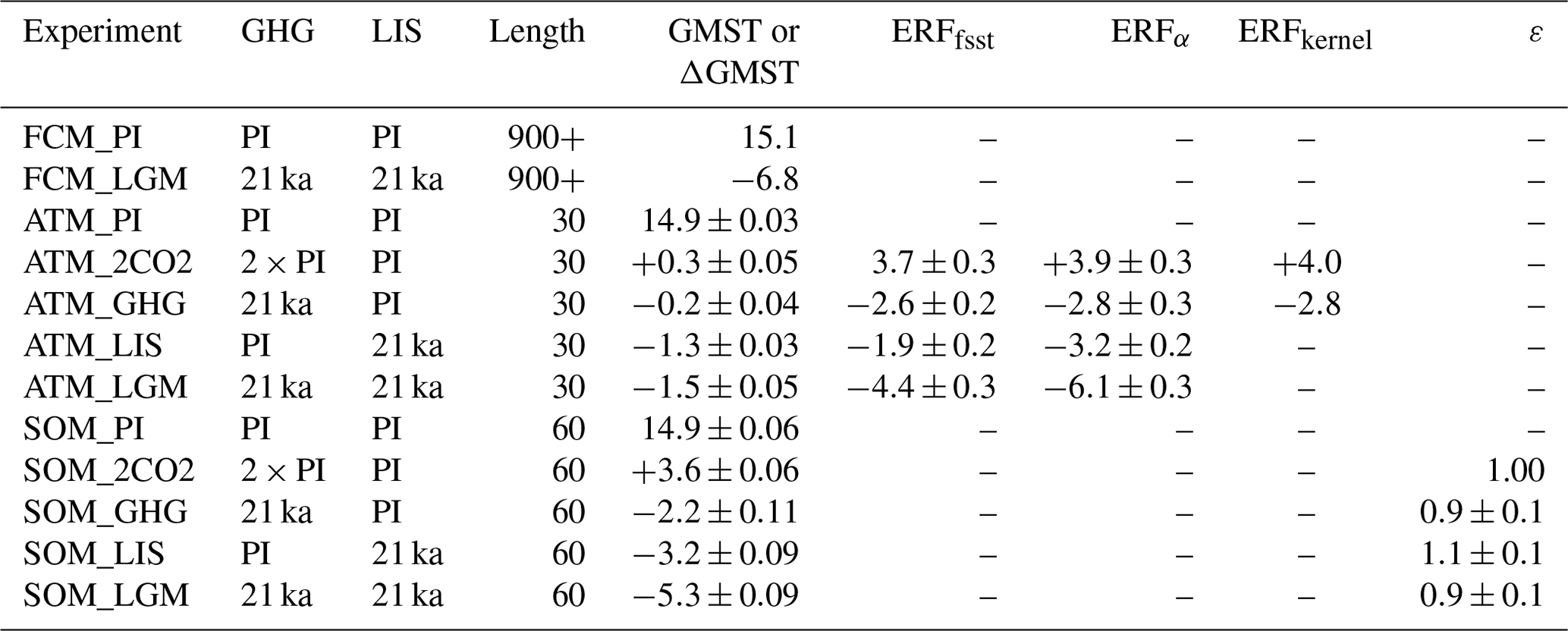
Equilibrium climate sensitivity (ECS) has been directly estimated using reconstructions of past climates that are different than today's. A challenge to this approach is that temperature proxies integrate over the timescales of the fast feedback processes (e.g., changes in water vapor, snow, and clouds) that are captured in ECS as well as the slower feedback processes (e.g., changes in ice sheets and ocean circulation) that are not. A way around this issue is to treat the slow feedbacks as climate forcings and independently account for their impact on global temperature. Here we conduct a suite of Last Glacial Maximum (LGM) simulations using the Community Earth System Model version 1.2 (CESM1.2) to quantify the forcing and efficacy of land ice sheets (LISs) and greenhouse gases (GHGs) in order to estimate ECS. Our forcing and efficacy quantification adopts the effective radiative forcing (ERF) and adjustment framework and provides a complete accounting for the radiative, topographic, and dynamical impacts of LIS on surface temperatures. ERF and efficacy of LGM LIS are −3.2 W m−2 and 1.1, respectively. The larger-than-unity efficacy is caused by the temperature changes over land and the Northern Hemisphere subtropical oceans which are relatively larger than those in response to a doubling of atmospheric CO2. The subtropical sea-surface temperature (SST) response is linked to LIS-induced wind changes and feedbacks in ocean–atmosphere coupling and clouds. ERF and efficacy of LGM GHG are −2.8 W m−2 and 0.9, respectively. The lower efficacy is primarily attributed to a smaller cloud feedback at colder temperatures. Our simulations further demonstrate that the direct ECS calculation using the forcing, efficacy, and temperature response in CESM1.2 overestimates the true value in the model by approximately 25 % due to the neglect of slow ocean dynamical feedback. This is supported by the greater cooling (6.8 ∘C) in a fully coupled LGM simulation than that (5.3 ∘C) in a slab ocean model simulation with ocean dynamics disabled. The majority (67 %) of the ocean dynamical feedback is attributed to dynamical changes in the Southern Ocean, where interactions between upper-ocean stratification, heat transport, and sea-ice cover are found to amplify the LGM cooling. Our study demonstrates the value of climate models in the quantification of climate forcings and the ocean dynamical feedback, which is necessary for an accurate direct ECS estimation.
- Article
(7683 KB) - Full-text XML
- BibTeX
- EndNote


Equilibrium climate sensitivity (ECS) is defined as the global mean surface air temperature (GMST) response to a doubling of atmospheric CO2 and accounts for the Planck response and water vapor, ice albedo, lapse rate, and cloud feedbacks (with timescales < 100 years; “Charney Sensitivity”; Charney et al., 1979). By tradition and for practical reasons, ECS does not account for slow feedback processes, such as changes in vegetation, cryosphere and ocean circulation, effects of which are included in Earth system sensitivity (e.g., Lunt et al., 2010). The ECS range is estimated to be 2.6–3.9 ∘C (66 % confidence interval) in a recent assessment (Sherwood et al., 2020), which represents a narrower range than the traditional one of 1.5–4.5 ∘C (IPCC, 2013). Nevertheless, ECS is difficulty to constrain from present-day observations due to the brevity of the instrumental record, the small magnitude of radiative forcing and temperature response relative to the natural variability, and the dependence of ECS estimates on the transient sea-surface temperature (SST) pattern in the historical period (Knutti et al., 2017; Sherwood et al., 2020).
Paleoclimate records overcome these limitations and provide unique observational constraints on ECS. The Last Glacial Maximum (LGM; ∼21 ka) has been considered to be an ideal target for estimating ECS since it represents a quasi-equilibrium climate state with large changes in climate forcing and response and relatively high spatial coverage of well-dated proxy temperatures. PALAEOSENS Project Members (2012) proposed a framework to obtain ECS from reconstructions of paleo-temperatures and climatic forcings in which slow (timescales > 100 years) feedback processes such as changes in greenhouse gases (GHGs), land ice sheets (LISs), Earth's orbits, and land use are regarded as climate forcings rather than feedbacks. This approach has been widely used to directly calculate ECS from proxy reconstructions of the LGM and glacial–interglacial cycles with estimates ranging from 2.6 to 8.1 ∘C (Friedrich et al., 2016; Köhler et al., 2017; Stap et al., 2019; Tierney et al., 2020; von der Heydt et al., 2014).
Direct ECS estimation using the PALAEOSENS Project Members (2012) approach relies on a complete understanding of the slow feedback processes. In the context of the LGM, both the radiative forcing due to changes in GHGs, LISs, vegetation, and aerosols and their efficacy (the ratio of the warming effect attributed to a given forcing relative to that due to a doubling of atmospheric CO2 under preindustrial conditions) must be known. Of these forcings, GHGs and LISs have been considered in most LGM-based ECS estimations (Friedrich et al., 2016; Köhler et al., 2017; Schmittner et al., 2011; Stap et al., 2019; Tierney et al., 2020; von der Heydt et al., 2014). Previous estimates of the LGM LIS forcing account for albedo changes associated with the presence of LISs and the exposure of shelves due to the lowered sea level (Fig. 1a), yielding a shortwave forcing ranging from −1.5 to −5.2 W m−2 (Braconnot et al., 2012; Braconnot and Kageyama, 2015; Friedrich et al., 2016; Hansen et al., 2013; Köhler et al., 2010; Taylor et al., 2007; Tierney et al., 2020). However, these estimates neglect changes in surface topography (Fig. 1b), which can change surface temperature and longwave emission. Moreover, LIS topographic changes altered atmospheric (Fig. 1c) and ocean circulations (Herrington and Poulsen, 2012; Kutzbach and Guetter, 1986; Zhu et al., 2014), which can change surface temperatures without directly involving radiative processes (e.g., through a wind–evaporation–SST feedback; Xie and Philander, 1994). To our knowledge, a complete quantification of the LGM LIS forcing that accounts for the radiative, topographic, and dynamical effects has not been done.
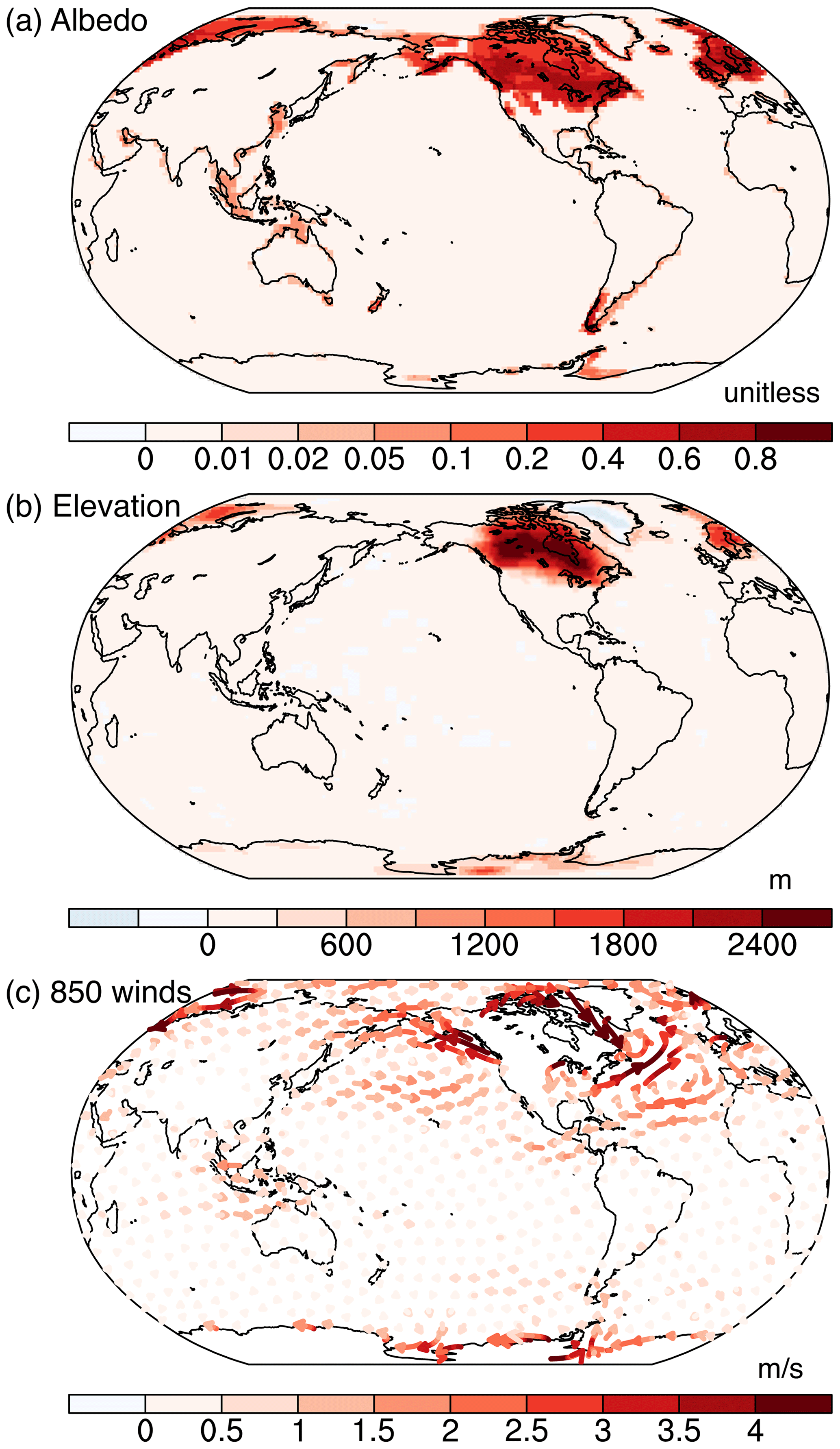
Figure 1(a) Changes in shortwave surface albedo associated with the presence of the LGM ice sheets and shelf exposures due to the lowered sea level. Albedo changes are diagnosed using “fixed-SST” experiments (ATM_LIS and ATM_PI; see Sect. 2.2). Note the uneven color bar. (b) Changes in surface elevation associated with the LGM ice sheets. (c) Wind changes at 850 hPa as an illustration of the ice-sheet dynamical forcing. Shown are anomalies in the fixed-SST experiments (ATM_LIS and ATM_PI).
Furthermore, the efficacy of LIS forcing has received relatively little attention (Yoshimori et al., 2009), although it is clear that albedo effects are mostly distributed over high-latitude land. This oversight is problematic since the assumptions of LIS efficacy can greatly impact the resulting ECS estimates (Stap et al., 2019; Tierney et al., 2020).
Another caveat with the direct ECS estimation approach is that fast feedbacks depend on the climate state and interact with slow feedbacks. Global climate model (GCM) studies have shown that the magnitude of fast climate feedbacks varies with global temperature, e.g., stronger cloud and water vapor feedbacks at higher GMSTs (Caballero and Huber, 2013; Schneider et al., 2019; Yoshimori et al., 2009; Zhu and Poulsen, 2020b; Zhu et al., 2019). Furthermore, the LGM ocean circulation was different than today (e.g., Curry and Oppo, 2005). Ocean dynamical processes can influence global temperature through interactions with sea ice, SST pattern, and cloud processes (Dong et al., 2019; Ferrari et al., 2014; Rose et al., 2014; Shin et al., 2003; Winton et al., 2013; Zhou et al., 2017), constituting an ocean dynamical feedback that takes place on timescales longer than 100 years. The contribution of the ocean dynamical feedback to the magnitude of LGM cooling and its impact on direct ECS estimation have not been thoroughly studied.
In this study, we address whether ECS can be accurately estimated using the direct calculation approach and knowledge of the LGM climate forcing and global temperature. To answer this question, we adopt the adjusted forcing–feedback framework (Sherwood et al., 2015) to provide a complete quantification of the forcing and efficacy of LGM LIS and GHG using a suite of climate simulations, in comparison to previous studies that only considered surface albedo effects of LIS. We also investigate the role of the ocean dynamical feedback in modulating the magnitude and spatial distribution of the LGM cooling by comparing fully coupled and slab ocean simulations. Finally, we discuss the implications of our results for direct ECS estimation using paleoclimate reconstructions.
2.1 Model and fully coupled simulations
We employ the Community Earth System Model (CESM) version 1.2 with a horizontal resolution of 1.9×2.5∘ (latitude × longitude) for the atmosphere and land and a nominal 1∘ for the sea ice and ocean (Hurrell et al., 2013). CESM1.2 is among the models that best reproduce climate features from instrumental records (Knutti et al., 2013) and has been extensively used for studying past climates (DiNezio et al., 2016; Otto-Bliesner et al., 2015; Zhu et al., 2017, 2019, 2020). Our CESM1.2 experiments were run with prescribed satellite phenology (SP) in the land model (Community Land Model version 4; CLM4) without an active carbon–nitrogen (CN) biogeochemical cycle. In the SP mode, leaf area and stem area indices and vegetation heights in CLM4 are prescribed according to data derived from satellite observations (Lawrence et al., 2011). Our choice of CLM4 with satellite phenology is based on the overall poorer simulation of vegetation phenology with an active CN, which could potentially be more problematic for paleoclimate simulations (Lawrence et al., 2011).
We make use of the fully coupled preindustrial (PI) and LGM simulations (FCM_PI and FCM_LGM; Table 1) from our previous studies (Tierney et al., 2020; Zhu et al., 2017). FCM_LGM was forced by boundary conditions consistent with protocols from the Paleoclimate Modelling Intercomparison Project phase 4 (PMIP4), including altered GHG concentrations, Earth orbital parameters, and LISs (Kageyama et al., 2017). LIS forcing is derived from the ICE-6G reconstruction (Peltier et al., 2015) and includes changes in land elevation and surface properties due to the presence of LGM ice sheets as well as changes in the land–sea mask to account for the lower sea level. FCM_LGM used prescribed preindustrial vegetation cover and aerosol emissions, as reliable global reconstructions are not available (Kageyama et al., 2017; Köhler et al., 2010). Although FCM_LGM contains the orbital forcing, its effect on GMST is small (e.g., Liu et al., 2014) and neglected in the following analysis. The FCM_LGM ocean state was initialized from the LGM simulation using the Community Climate System Model version 4, which had been spun-up for more than 2400 years and reached a quasi-equilibrated state (Brady et al., 2013). FCM_LGM was integrated for an additional ∼1800 years to reach equilibration under an updated atmosphere model (DiNezio et al., 2016; Tierney et al., 2020; Zhu et al., 2017). The top-of-atmosphere (TOA) energy imbalance averaged over the last 100 years is −0.06 W m−2 in FCM_LGM, which is comparable to the 0.09 W m−2 in FCM_PI, indicating the surface climate has reached a quasi-equilibrium glacial state. The global volume-mean ocean temperature exhibited a cooling of 0.15 ∘C in the last 900 years of FCM_LGM. GMST in FCM_LGM is 6.8 ∘C lower than that in FCM_PI and falls within the range directly estimated from proxy data in a recent study (−6.8 to −4.4 ∘C; Tierney et al., 2020).
Table 1List of CESM simulations conducted in this study, including experiment name, climate forcing configurations, run length (years), GMST and GMST changes (∘C), effective radiative forcing (ERF; W m−2), and efficacy (unitless). One standard deviation calculated using annual data is listed. Note that kernel-corrected ERF uses 12-month climatology and no uncertainty is provided.
2.2 “Fixed-SST” simulations and the effective radiative forcing
We adopt the forcing–feedback framework with the concept of rapid adjustments (Sherwood et al., 2015). We use fixed-SST experiments to calculate the effective radiative forcing (ERF), defined as the change in net TOA radiative flux after adjustments of the atmospheric temperature profile, water vapor, and clouds (Hansen et al., 2005). Our results show that this method is especially well-suited for quantifying the LIS forcing and is an advancement over either simplified bulk calculations or the approximate partial radiative perturbation method used in previous studies, which only provide an estimation of the shortwave forcing from albedo effects. In the fixed-SST experiments, an LGM climate forcing (e.g., GHG) is introduced into a preindustrial simulation with active atmosphere and land models, but with SST and sea ice prescribed to the unperturbed preindustrial climatology. The land surface temperature is allowed to adjust as it is impractical to fix in the model. The ERF attributed to a forcing is obtained as the change in TOA net radiation between simulations with and without the forcing. ERF and land temperature change in the fixed-SST experiments are termed ERFfsst and ΔTfsst, respectively. Changes in atmospheric temperature, water vapor, and clouds in response to the climate forcing, without mediation by the global-mean temperature, are referred to as “adjustments” (see Fig. 1 of Sherwood et al. (2015) for an illustration).
To quantify the ERF due to LGM LIS and GHG, we performed two fixed-SST experiments with LGM GHG and LIS forcing, respectively (ATM_GHG and ATM_LIS; Table 1). To examine whether ERFs from GHG and LIS are additive, we performed an additional experiment with both forcings included (ATM_LGM). To compare the forcing and response of LGM GHG and LIS to CO2 increasing, we also carried out an experiment with twice the preindustrial atmospheric CO2 concentration (ATM_2CO2). Finally, a standard preindustrial atmosphere-only simulation was performed and used as a reference (ATM_PI). These fixed-SST experiments used the same set of preindustrial SST and sea-ice coverage derived from the FCM_PI climatology. All fixed-SST simulations were run for 30 years with the last 25 used for analysis.
ERFfsst contains radiation changes (biases) resulting from land surface temperature changes (ΔTfsst). For example, ΔTfsst is negative in ATM_GHG (see Fig. 2a), leading to an underestimation of the magnitude of ERF due to the decrease in Planck emission at lower land surface temperatures. To account for the radiative effects from ΔTfsst, two corrected versions of ERF were computed. In the first, the ΔTfsst effect on TOA radiation was corrected using the climate sensitivity parameter (α; units: K W−1 m−2) as
α was obtained from the coupled simulation in a slab ocean configuration (see Sect. 2.3). In the second correction, radiative kernels were used:
In this approach, ERFkernel is obtained by subtracting the direct rapid adjustments associated with ΔTfsst from ERFfsst while keeping the indirect rapid adjustments, such as cloud responses (Tang et al., 2019). The direct rapid adjustments that are subtracted include effects over land from changes in surface temperature (ATs), tropospheric air temperature (ATa), tropospheric water vapor (Aq), and albedo (Aalb). ATa is calculated by assuming a constant lapse rate in the troposphere, i.e., the same tropospheric air temperature change as the surface. Similarly, Aq accounts for the effect from tropospheric water vapor change under the assumption of a constant lapse rate. Aq is calculated by scaling the total water vapor effect with the ratio between the temperature-induced radiative flux change from a constant lapse rate and that from the full tropospheric temperature change.
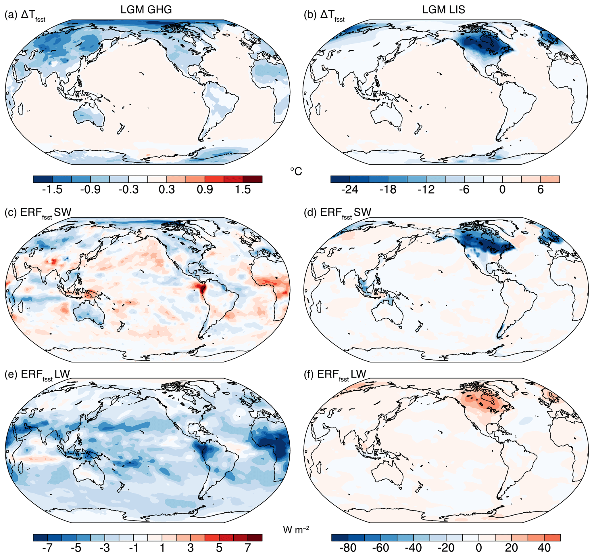
Figure 2(a) Land surface temperature changes (ΔTfsst) in response to the LGM GHG forcing diagnosed in “fixed-SST” experiment ATM_GHG. (b) ΔTfsst in response to the LGM LIS forcing diagnosed in ATM_LIS. (c) The shortwave component of effective radiative forcing associated with LGM GHG forcing diagnosed in ATM_GHG. (e) As (c) but for the longwave component. (d, f) As (c, e) but for the LGM LIS forcing. Note that a present-day land–sea mask is shown in all the figures, which differs from the LGM mask due to a lower sea level; this will result in a temperature difference over the shelf exposure regions in (b). Surface temperature above sea ice is allowed to adjust in fixed-SST experiments.
2.3 Slab ocean model simulations and the efficacy of forcing
To compare temperature responses to different climate forcings and to estimate α, we performed sensitivity experiments in a slab ocean model (SOM) configuration without ocean dynamics (Table 1). The SOM uses prescribed mixed-layer depth and heat transport convergence (“q flux” hereafter) (Bitz et al., 2011) that are derived from FCM_PI. As a result, temperature responses in SOM simulations are caused by the fast feedback processes and exclude the ocean dynamical feedback. SOM_GHG includes LGM GHG levels and the preindustrial values of all the other boundary conditions. Similarly, SOM_LIS incorporates the LGM ice-sheet forcing including a higher topography, an altered land–sea distribution to account for effects from sea-level change, and modified land surface properties over ice sheets. To examine whether the climate responses are additive, we performed SOM_LGM, in which both LGM GHG and LIS forcings were added. In addition, we conducted SOM_2CO2 with CO2 level 2 times the preindustrial value. These SOM simulations were integrated for 60 years to allow the model to reach equilibrium (with TOA energy imbalance < 0.1 W m−2) (Danabasoglu and Gent, 2009). Averages over the last 20 years are used for analysis.
The climate sensitivity parameter (α) was obtained from fixed-SST and SOM simulations and used to calculate ERFα (Eq. 1). Specifically, for a climate forcing (GHG, LIS, or 2×CO2), α was estimated as
ΔTSOM is the equilibrated GMST response in the SOM simulation. ΔTSOM−ΔTfsst represents the SST-mediated surface air temperature changes that are associated with ERFfsst.
We define the efficacy (ε) of a climate forcing (GHG or LIS) as a ratio of its temperature response scaled by its ERFα to that of 2×CO2:
We note that the LGM GHG forcing and efficacy in this study are calculated using a “low-top” atmosphere model with prescribed stratospheric chemical tracers and exclude indirect effects from stratosphere chemistry (Hansen et al., 2005).
2.4 The radiative kernels and approximate partial radiative perturbation approach
To correct the ERFs of doubling CO2 and LGM GHG and to understand their efficacy, we employ the radiative kernels that are developed for CESM (Pendergrass et al., 2018). In the analysis, we calculate changes in the 12-month climatology of the variable of interest (e.g., surface temperature) and multiply that by the corresponding radiative kernel to estimate the TOA radiation changes. Climate feedback parameters are obtained by normalizing the TOA radiation anomalies by the GMST changes. Kernels analyses are not performed for LGM LIS simulations, as the present-day kernels are not suitable due to the large difference in the characteristics of the forcing and response (Yoshimori et al., 2011).
The approximate partial radiative perturbation (APRP; Taylor et al., 2007) is used to quantify the shortwave forcing and feedback, in particular for the LIS simulations. In contrast to the radiative-kernel method, APRP is independent of the forcing and background climate state and produces results that differ from partial radiative perturbation (PRP) by less than 7 % (Taylor et al., 2007; Yoshimori et al., 2011; Zhu and Poulsen, 2020b; Zhu et al., 2019). APRP represents the atmosphere as a single layer with bulk optical properties and usually uses monthly mean model output to derive the radiative effects and feedbacks associated with changes in surface albedo, clear-sky processes, and clouds. The shortwave cloud feedback is further decomposed into contributions from changes in cloud amount, scattering, and absorption. APRP has been used in many previous studies to quantify the shortwave forcing associated with LIS albedo changes (Braconnot et al., 2012; Braconnot and Kageyama, 2015; Brady et al., 2013; Taylor et al., 2007; Tierney et al., 2020). When using APRP to quantify shortwave feedbacks, we only show results over model grid points that are ocean in both PI and LGM simulations; in this way, climate feedbacks are separated from forcings, e.g., from LIS, although feedback processes over land are overlooked.
3.1 Effective radiative forcing
The ERFfsst due to LGM GHG is W m−2 (±1σ; Table 1; Fig. 2c and e). After correcting the radiative effects associated with land temperature changes ( ∘C; Fig. 2a) using the climate sensitivity parameter and radiative kernels, the ERFα and ERFkernel are and −2.8 W m−2, respectively, and agree well with previous estimates of −2.8 to −3.0 W m−2 (Hansen et al., 2013; Köhler et al., 2010). For a doubling of CO2, ERFfsst, ERFα, and ERFkernel are 3.7±0.3, 3.9±0.3, and 4.0 W m−2, respectively, well within the multi-model range in recent studies (Smith et al., 2018; Tang et al., 2019). For both LGM GHG and 2×CO2, ERFkernel falls in the middle of the uncertainty range of ERFα, suggesting that both the correction methods using radiative kernels and climate sensitivity parameters produce meaningful and accurate results.
In response to LGM LIS, ΔTfsst has a global mean of −1.3 ∘C with maximum cooling over ice sheets exceeding −24 ∘C, much greater than the land temperature changes associated with GHG forcing (Table 1; Fig. 2a and b). ΔTfsst results from the higher surface albedo over regions with increased coverage of ice sheets and land (due to shelf exposures), the elevated ice-sheet topography, and radiative and dynamic atmospheric adjustments. The global mean ERFfsst due to LGM LIS is W m−2, resulting from a shortwave component of −3.7 W m−2 (ERFfsst_sw; Fig. 2d) and a longwave component of 1.8 W m−2 (ERFfsst_lw; Fig. 2f). ERFfsst_sw is lowest over ice sheets with values of less than −80 W m−2. Using shortwave APRP, we attribute 77 % (−2.8 W m−2) of ERFfsst_sw to surface albedo changes over regions of ice sheets and shelf exposure, 13 % (−0.5 W m−2) to surface albedo changes associated with snow cover increases outside the ice-sheet regions, and 8 % (−0.3 W m−2) to cloud adjustments. The majority of the cloud adjustments (−0.2 W m−2) occurs over the Indo-Pacific warm pool, where the exposure of the Sunda and Sahul shelves produces a surface cooling and drying (DiNezio et al., 2016) and increases cloud condensates through enhanced large-scale moist advection (Zhang et al., 2003). Outside the tropics, clouds diminish over ice sheets and in the downwind regions and shift with the position of the storm tracks; yet, the overall impact on the global mean ERFfsst_sw is small. ERFfsst_lw exceeds 40 W m−2 over ice sheets, which results primarily from the reduced longwave radiation due to a higher effective emission elevation and lower temperatures (Figs. 1b and 2b).
Using the climate sensitivity parameter (diagnosed in SOM_LIS; Table 1; Eqs. 1 and 3), we calculate a global mean ERFα from LGM LIS of W m−2. Our calculation accounts for the radiative, topographic, and dynamic adjustments associated with LIS, in contrast to only the albedo effects considered in previous studies (Braconnot et al., 2012; Braconnot and Kageyama, 2015; Taylor et al., 2007; Tierney et al., 2020). Using the APRP approach as in these previous studies, we calculate a shortwave forcing of −2.8 W m−2 from surface albedo changes over regions with new ice-sheet coverage and shelf exposures in ATM_LIS. We note that this APRP approach overestimates the shortwave radiative forcing that is attributable exclusively to changes in LIS extent, as it includes the radiative effect of snow increases over ice sheets (or regions with shelf exposure); the albedo of fresh snow is considerably larger (0.8–0.9 versus ∼0.6) (Cuffey and Paterson, 2010). The LIS-induced cooling increases the proportion of snow relative to rain, which reflects more shortwave radiation than that from ice-sheet albedo alone. The snow-induced overestimation of the LIS forcing is larger if the cooling over ice sheets is greater. For example, the shortwave forcing from APRP analysis is greater in coupled simulations than that in atmosphere-only simulations with fixed PI SST (e.g., −3.3 W m−2 in FCM_LGM versus −2.8 W m−2 in ATM_LIS), due to the greater cooling over ice sheets.
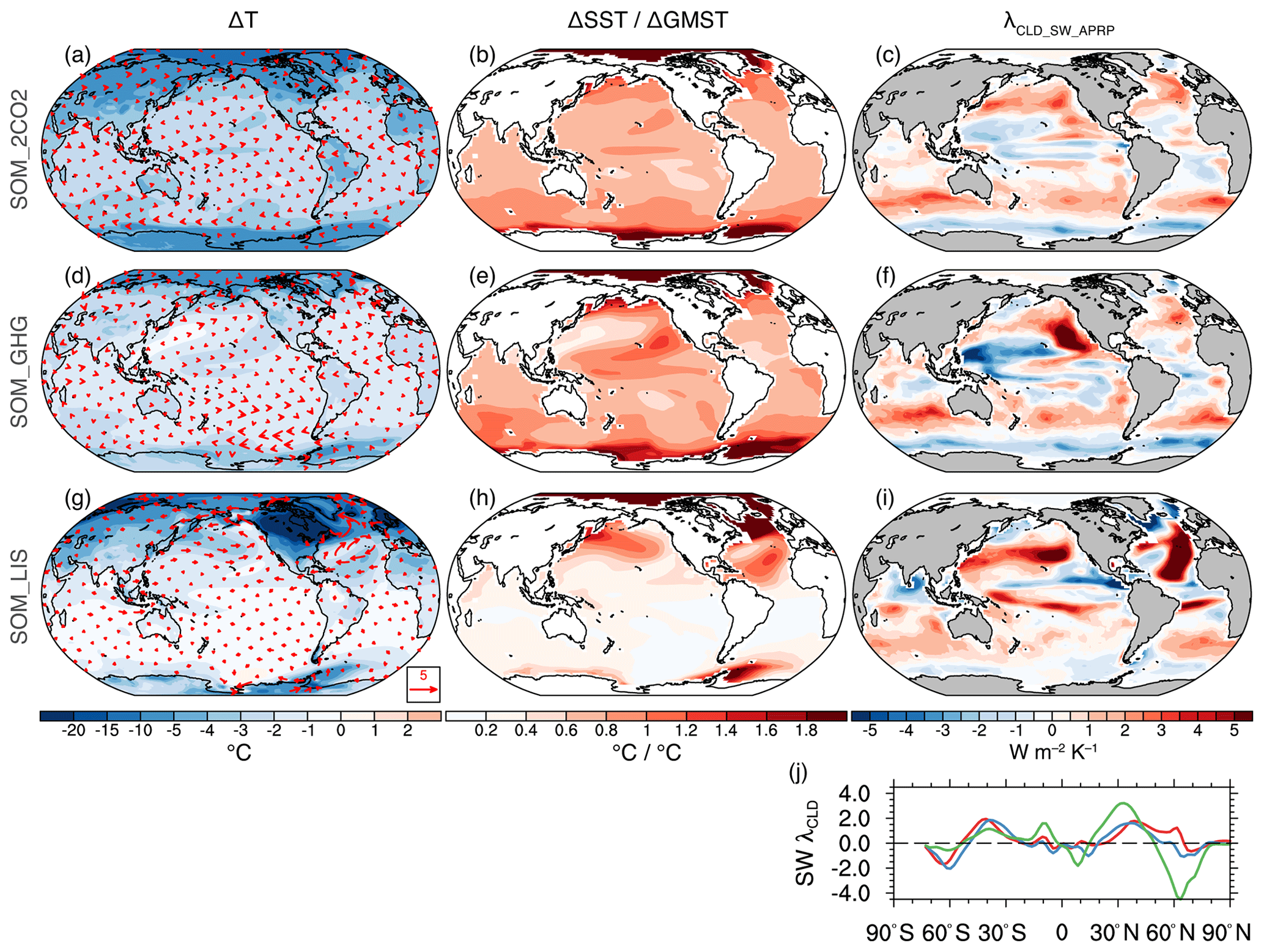
Figure 3Changes in surface temperature in (a) SOM_2CO2, (d) SOM_GHG, and (g) SOM_LIS. Changes in 850 hPa winds (units: m s−1) in fixed-SST experiments are shown as vectors in (a) ATM_2CO2, (d) ATM_GHG, and (g) ATM_LIS. Changes in SST scaled by the corresponding GMST change in (b) SOM_2CO2, (e) SOM_GHG, and (h) SOM_LIS. The shortwave cloud feedback parameter over LGM ocean grid points diagnosed using the APRP approach in (c) SOM_2CO2, (f) SOM_GHG, and (i) SOM_LIS. (j) Zonal mean shortwave cloud feedback over ocean in SOM_2CO2 (red), SOM_GHG (blue), and SOM_LIS (green). Note that temperature and wind changes in 2×CO2 experiments in (a) have been multiplied by −1 to facilitate the comparison with those in SOM_GHG and SOM_LIS.
3.2 Efficacy of LGM GHG and LIS forcings
Our results suggest that the efficiency of lowering GHGs to LGM levels is smaller than that of doubling atmospheric CO2 under PI conditions, i.e., the LGM GHG forcing has a smaller-than-unity efficacy of 0.9±0.1 (Table 1; Eq. 4). In SOM_2CO2, GMST increases by 3.6 K in response to an ERFα of 3.9 W m−2. In SOM_GHG, GMST decreases by 2.2 K in response to an ERFα of −2.8 W m−2. The lower ε of LGM GHG forcing is caused by a weaker cloud feedback in response to cooling (Table 2). Using radiative kernels, we find that the Planck, albedo, and combined lapse rate and water vapor feedbacks stay largely unchanged; however, the cloud feedback parameter is 30 % smaller in SOM_GHG than in SOM_2CO2 (0.32 versus 0.46 W m−2 K−1). The decrease in the cloud feedback is due to the shortwave component; the cloud scattering feedback is weaker in response to cooling than that to warming over high-latitude regions, leading to a weaker shortwave response (Fig. 3c, f and j; Table 2 APRP columns). These results demonstrate a state-dependent cloud feedback that increases with GMST, a feature that has been found in the latest three CAM versions (Zhu and Poulsen, 2020b; Zhu et al., 2019) and many other climate modes (e.g., Crucifix, 2006).
Table 2Climate feedback parameters (units: W m−2 K−1) in the SOM simulations. Radiative-kernel-based analysis is performed for SOM_2CO2 and SOM_GHG but not SOM_LIS due to the drastically different boundary conditions. APRP-based analysis is performed for all three simulations. APRP quantifies the shortwave climate feedback parameter and decomposes the cloud feedback into contributions from changes in cloud amount, scattering, and absorption. The cloud absorption feedback is not shown, as it is small and varies little between simulations. Values in parentheses are the contribution to the global mean value from ocean grid points in LGM simulation. Note that the high value in the albedo column for SOM_LIS (1.31) includes the contribution from the shortwave forcing over land.
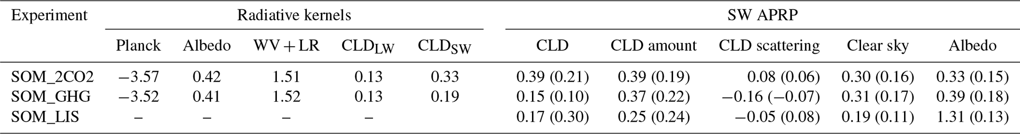
The ε of LGM LIS is 1.1±0.1, resulting from an ERFα of −3.2 W m−2 and a ΔGMST of −3.2 K in SOM_LIS (Table 1) and suggesting that LIS forcing is 10 % more effective in changing GMST than doubling CO2 when only fast feedbacks are considered. Overall, 40 % of the LIS-induced cooling (1.3 of 3.2 K) is attributed to land temperature changes that involve radiative, topographic, and dynamical effects of the LIS forcing and are independent from SST changes (Figs. 1 and 2; Table 1); land only accounts for 7 %–8 % of the GMST change in SOM_2CO2 and SOM_GHG. In addition to the large contribution from processes over land, the shortwave cloud feedback over ocean is greater in response to the LIS forcing (0.30 W m−2 K−1) than that to the doubling CO2 forcing (0.21 W m−2 K−1; APRP analysis in Table 2 and Fig. 3). The greater shortwave cloud feedback is due to changes in both cloud amount and scattering and is especially prominent over the Northern Hemisphere subtropics (Fig. 3j), which likely reflects the southward shift of storm tracks and clouds. The process can also be understood as an “SST pattern effect”. The cloud feedback parameter is expressed as
where SSTSUB is the SST over the subtropical North Pacific and North Atlantic, and CRE denotes the global cloud radiative effects. SSTSUB is positively correlated with global CRE () (Dong et al., 2019; Zhou et al., 2017). As a result, a greater SSTSUB change relative to the GMST gives rise to greater cloud feedback through changing the lower-tropospheric stability (Wood and Bretherton, 2006). Over the subtropical North Pacific and North Atlantic, the shortwave cloud feedback exceeds 10 W m−2 K−1 in SOM_LIS, in comparison to a maximum of ∼3 W m−2 K−1 in SOM_2CO2 (Fig. 3c and f), which is consistent with the relative magnitude of SST change in each experiment (Fig. 3b and h).
The formation of the SST responses over the subtropical North Pacific and North Atlantic is attributed to the ice-sheet-driven wind changes (Fig. 3g). In response to the topographic effects of LGM LIS, the Northern Hemisphere westerly jet shifts southward in ATM_LIS, producing cyclonic low-level wind anomalies over the subtropical and midlatitude North Pacific and anticyclonic anomalies over the subtropical North Atlantic (Kutzbach and Guetter, 1986; Zhu et al., 2014). This anomalous wind pattern forces regional SST changes through changing latent heat flux and amplify the coupled response through the wind–evaporation–SST feedback (Chiang and Bitz, 2005; Xie and Philander, 1994). For example, the trade wind strengthens over the subtropical North Atlantic, which cools the subtropical SST due to the enhanced evaporation and reinforces the anomalous wind pattern, forming a positive feedback. This non-radiative pathway of LIS's influence on the surface temperature is largely absent when GHGs are changed (Fig. 3a and d), highlighting the complex nature of non-GHG climate forcings and the importance of using efficacy to evaluate the overall effectiveness of their radiative forcing as compared to a doubling of atmospheric CO2.
3.3 Are forcings and responses additive?
Our simulations suggest that ERFs and surface temperature responses of LGM GHG and LIS are globally additive. In fixed-SST experiments with both the LGM GHG and LIS forcings (ATM_LGM), ERFfsst is W m−2, approximately the sum of those in ATM_GHG and ATM_LIS ( and , respectively). Similarly, the ERFα in ATM_LGM, W m−2, is nearly equal to the sum of those in ATM_GHG and ATM_LIS ( and W m−2, respectively). The SOM_LGM ΔGMST in response to combined GHG and LIS forcings is ∘C and is close to the sum of ΔGMSTs in SOM_GHG and SOM_LIS ( and ∘C, respectively). From these results, we conclude that ERF and ΔGMST due to individual forcings are additive at the global level, which supports the approach to separate the LGM climate forcing and response into components associated with individual forcing agents. We note that at the regional level, especially over high latitudes, the ERF and ΔGMST from the sum of individual forcings and combined forcings do not match as well as at the global level (figure not shown), likely due to local feedbacks related to sea ice. It remains unclear whether the temperature responses to individual forcings are additive when slow feedback processes (e.g., ocean dynamics) are included.
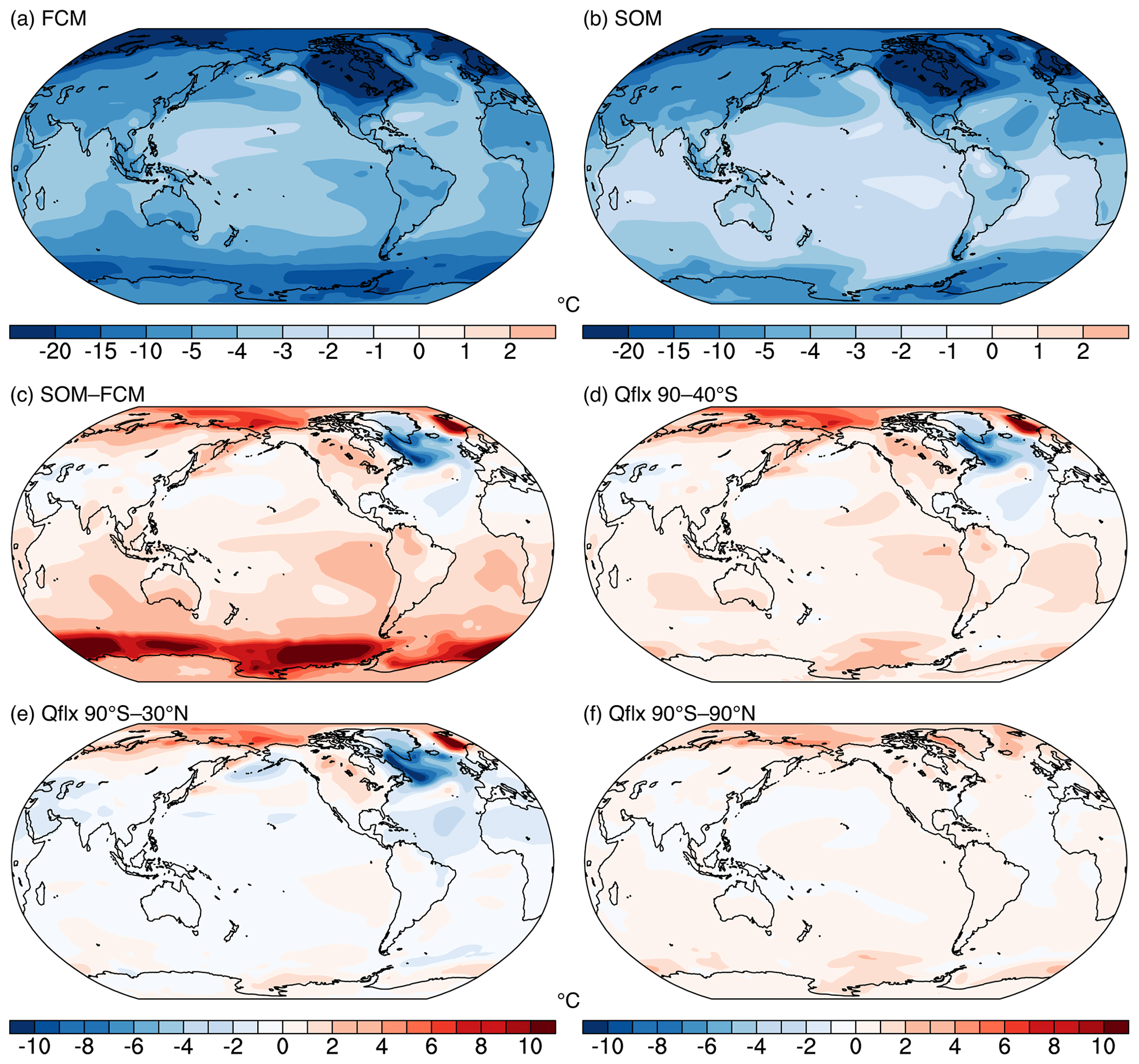
Figure 4(a) LGM cooling in the fully coupled model simulations (FCM_LGM–FCM_PI). (b) LGM cooling in the slab ocean model simulations (SOM_LGM–SOM_PI). Both SOM_LGM and SOM_PI use the same ocean mixed-layer depth and heat flux convergence (Qflx) that are derived from the fully coupled preindustrial simulation (FCM_PI). (c) Difference in the simulated LGM cooling between SOM and FCM (a, b). (d) As (c) but for the SOM simulation with the prescribed Qflx over the Southern Ocean (90–40∘ S) replaced with that from FCM_LGM. (e) As (c) but for the SOM simulation with the prescribed Qflx over 90∘ S–30∘ N replaced with that from FCM_LGM. (f) As (c) but for the SOM simulation with the prescribed Qflx over the global ocean replaced with that from FCM_LGM. Note that a small intrinsic bias in surface temperature associated with SOM simulations (e.g., SOM_PI–FCM_PI) has been subtracted when comparing SOM and FCM simulations.
3.4 The ocean dynamical feedback
Our results demonstrate that the full extent of LGM cooling cannot be produced using an SOM configuration that accounts for fast feedback processes but excludes the slow ocean dynamical changes. ΔGMST is −6.8 ∘C in FCM_LGM and −5.3 ∘C in SOM_LGM (Table 1; Fig. 4a and b). Both simulations have reached an equilibrium state at the surface under the same climate forcings and only differ in the complexity of the ocean model. The LGM cooling is 1.5 ∘C (28 %) greater with active ocean dynamics and interactions with the atmosphere and sea ice. The difference in LGM cooling between SOM and FCM primarily occurs in the Southern Ocean (SO), where SOM_LGM simulates a weaker LGM cooling by more than 10 ∘C (Fig. 4a–c). In the eastern equatorial Pacific and eastern subtropical oceans (except for the subtropical Atlantic), SOM_LGM simulates a smaller LGM cooling by 1–2 ∘C. In the North Atlantic, LGM cooling in SOM_LGM is greater by ∼1 ∘C in the subtropics and more than 5 ∘C along the sea-ice margin in subpolar regions. Over the Indo-Pacific Warm Pool and the western subtropics, surface temperature change is similar between FCM and SOM simulations, suggesting a limited role of ocean dynamical response over these regions.
Accounting for the SO dynamical effects increases the LGM cooling in the SOM configuration and explains the majority (67 %) of the difference from FCM simulations. This is shown in an LGM SOM simulation (SOM_SO), in which the prescribed q flux over the SO (90–40∘ S) is replaced with those derived from FCM_LGM, with other regions remaining unchanged (using values from FCM_PI). SOM_SO simulates a colder LGM than SOM_LGM, especially over the SO, where the large temperature difference (>10 ∘C) between SOM_LGM and FCM_LGM is mostly removed (Fig. 4d versus Fig. 4c). In addition to the impact on local temperatures, SOM_SO simulates lower surface temperatures over the eastern equatorial Pacific and Indian Ocean and the Southern Hemisphere subtropics, producing a better match with FCM_LGM over these regions. This reflects a remote impact of the SO processes on the lower latitudes through changing tropical atmospheric circulations (Hwang et al., 2017).
The SO dynamical effects primarily result from upper-ocean stratification changes and the coupling with sea ice. In FCM_PI, the SO is stratified with the maximum ocean temperature occurring in the subsurface (500–1000 m; Fig. 5a). In zonal and annual mean, isotherms (shadings in Fig. 5a) intersect isopycnals (contours) mostly near 65–60∘ S and along the Antarctic coast, indicating strong heat diffusion towards the mixed layer, i.e., a heat flux convergence of approximately −20 W m−2 (Fig. 5c; red curve). The strong heat flux convergence warms the mixed layer and inhibits sea-ice formation, resulting in a quasi-permanent sea-ice extent to 68∘ S (red horizontal bar in Fig. 5c; defined using a 70 % annual mean sea-ice cover). In comparison, the upper-ocean stratification in FCM_LGM is greatly reduced with a potential density change of less than 0.4 kg m−3 over most water columns and a largely invariant ocean temperature of −2 ∘C (Fig. 5b). Meanwhile, the center of mixed-layer heat flux convergence is shifted northward to ∼56∘ S and the quasi-permanent sea ice expands to ∼58∘ S (Fig. 5c). An initial LGM cooling in the SO (e.g., caused by fast feedback processes) increases sea-ice formation and brine rejection, which enhances convection and decreases the upper-ocean stratification, resulting in a decrease in heat flux convergence to the mixed layer and amplifying sea-ice expansion. This feedback loop is absent in an SOM configuration with prescribed mixed-layer depth and heat flux convergence, leading to little expansion of the quasi-permanent sea ice (cyan horizontal bar in Fig. 5c) and much less LGM cooling in SOM_LGM (Fig. 4b and c). When the LGM changes in mixed-layer depth and heat flux convergence are prescribed in SOM_SO, sea ice expands northward (light green bar in Fig. 5c) and the SO experiences cooling (Fig. 4d versus Fig. 4c).
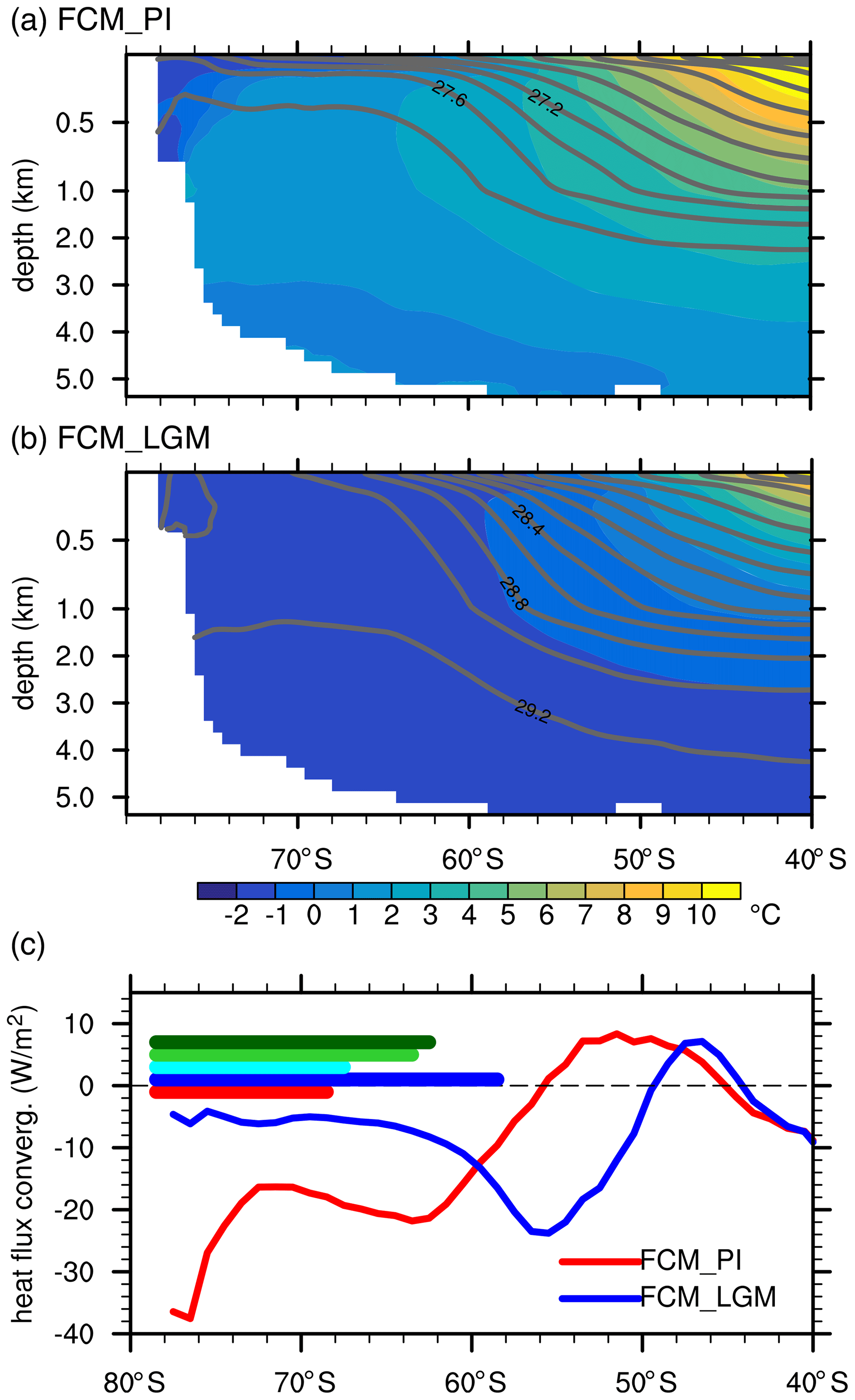
Figure 5(a) Zonal mean potential temperature (shadings; units: ∘C) and potential density (contours) over the Southern Ocean in the fully coupled preindustrial simulation (FCM_PI). Potential density values are reported in kilograms per cubic meter subtracting 1000 kg m−3. (b) As (a) but for the fully coupled LGM simulation (FCM_LGM). (c) Zonal mean heat flux convergence (units: W m−2) in the ocean mixed layer in FCM_PI (red) and FCM_LGM (blue). Negative values indicate that ocean dynamical processes transport heat from below into the mixed layer. Horizonal bars indicate the zonal mean semi-permanent sea-ice extent, defined as a 70 % of the annual mean sea-ice cover, in the FCM_PI (red), FCM_LGM (blue), SOM_LGM (cyan), and SOM simulations with Qflx over 90–40∘ S (light green) or 90∘ S–30∘ N (dark green) replaced with that in FCM_LGM.
Accounting for additional ocean dynamical effects in the low latitudes and the Northern Hemisphere further decreases the difference in LGM cooling between SOM and FCM simulations. This is supported by additional SOM simulations, in which we replace the prescribed q flux with those derived from FCM_LGM over 90∘ S–30∘ N and the entire global ocean. The tropical ocean dynamical effects decrease SST in the eastern equatorial Pacific and the Southern Hemisphere subtropics (Fig. 4e). Ocean dynamics in the Northern Hemisphere middle and high latitudes increases SST over the North Atlantic (Fig. 4f). The tropical ocean dynamical effects primarily result from changes in tropical ocean circulations and the coupling with the atmosphere (DiNezio et al., 2011; Vecchi and Soden, 2007). The Northern Hemisphere ocean dynamical effects are related to a stronger Atlantic Meridional Overturning Circulation (AMOC) and a greater northward ocean heat transport in the model (Brady et al., 2013). After accounting for the global ocean dynamical effects by using the q flux derived from FCM_LGM, high-latitude oceans still exhibit a temperature difference of ∼1–2 ∘C, contributing to a GMST of ∼0.3 ∘C, likely reflecting the challenge of using prescribed q flux to approximate the full extent of ocean dynamical effects (Bitz et al., 2011). Nevertheless, these results highlight the important role of the slow ocean dynamical feedback in modulating regional and global temperatures.
Results presented herein highlight major caveats of the direct ECS estimation approach. Firstly, a complete understanding of the magnitude and efficacy of forcing agents is necessary, especially for non-GHG forcings (e.g., LIS, vegetation, and aerosols) that may have distinct spatial distribution and non-radiative pathways to change the energy balance of Earth. We suggest a GCM-based approach using the effective radiative forcing and adjustment framework to account for the complicated aspects of paleoclimate non-GHG forcings. In this approach, a fixed-SST simulation of ∼30 years with a forcing of interest is first conducted to calculate the effective radiative forcing (ERFfsst) and the associated land temperature changes. An ERFα is then obtained by correcting the ERFfsst using the climate sensitivity parameter that is derived in an additional SOM simulation of ∼60 years. Moreover, efficacy of the forcing can also be derived using these simulations. This approach provides a complete consideration of the radiative and non-radiative effects of the forcing agent and is more consistent with the basic definition of the forcing–feedback framework. In contrast, the APRP-based approach used in previous studies only accounts for the effects from albedo changes. We note that, due to the inclusion of snow effects in the forcing quantification, the APRP-based approach overestimates the direct shortwave albedo effects that are attributable only to changing LIS extent. Our simulations suggest an LGM LIS efficacy of 1.1, which differs from the 0.45 in Stap et al. (2019). A precise explanation about this difference is challenging, given the large differences in the definition of forcing or efficacy, model complexity, and experimental design. Future studies are needed to quantify the effective radiative forcing and efficacy of the LGM vegetation and aerosols, as they are prescribed at the preindustrial values in our LGM simulations.
A second caveat concerns the role of the ocean dynamical feedback, which occurs on timescales of 102–103 years and should be accounted for when directly estimating ECS using forcing or response of an equilibrium climate. This complication stems from defining ECS to include only fast feedback processes with timescales of less than 100 years. Ocean feedback processes, including the heat redistribution by ocean circulation and the coupling with the atmosphere or sea ice, require more than 100 years to develop. Reconstructions of past climate forcings and GMST usually do not directly constrain ocean circulations and therefore could potentially impact the ECS estimation.
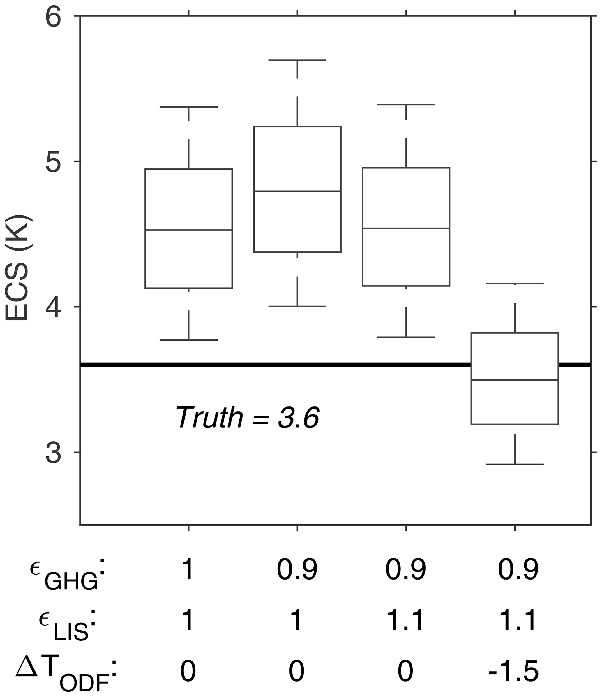
Figure 6ECS in CESM1.2 (horizontal line) and the LGM-based estimates (box-and-whisker plots) using different values of forcing efficacy and ocean dynamical feedback (ODF)-induced ΔGMST changes. Each ECS estimation is obtained by performing 10 000 Monte Carlo calculations, which incorporates the uncertainties (assumed to be Normal) in forcings and temperature responses. The box and whisker indicate a 68 % and 95 % confidence interval, respectively. ERFs and efficacy of LGM GHG and LIS are listed in Table 1. ΔGMST changes from the ocean dynamical feedback is the difference between FCM and SOM simulations (Table 1).
To demonstrate the above caveats, we assume CESM1.2 is a perfect model and estimate ECS using LGM constraints that are derived from model simulations as
In the above equation, ΔGMSTODF denotes the GMST change (approximately −1.5 ∘C; see Sect. 3.4) that is caused by the slow ocean dynamical feedback and is subtracted from the total LGM cooling (ΔGMST = −6.8 ∘C in CESM1.2). ERFGHG, ERFLIS, and ERF in our simulations are , , and 3.9±0.3 W m−2, respectively (Table 1). εGHG and εLIS are 0.9 and 1.1, respectively. In our “perfect model” assumption, all the above values are unbiased, and the “true” ECS is 3.6 ∘C. We perform ECS calculations using Eq. (6) with 10 000 Monte Carlo draws to sample the uncertainty in forcings and explore impacts from different assumptions of climate forcing or efficacy and the ocean dynamical feedback (Fig. 6). If we do not remove the effects of the ocean dynamical feedback and assume that both GHG and LIS forcings have a unit efficacy, as has been done in most previous studies (e.g., PALAEOSENS Project Members, 2012), we obtain a median ECS of 4.5 ∘C, an overestimate of 25 % that is statistically distinguishable from uncertainties associated with climate forcings. Using the true efficacy of the LGM GHG or LIS produces a small change in ECS ( ∘C) that approximately cancels each other, as εGHG is smaller and εLIS is larger than unity. Accounting for the ocean dynamical feedback greatly improves the ECS calculation, yielding a median of 3.5 ∘C, 0.1 ∘C smaller than the true ECS. We note that here we account for the ocean dynamical effect by subtracting the corresponding contribution from the total LGM GMST change. Alternatively, we can also invoke a non-constant sea-ice albedo feedback that depend on ocean dynamics (see Fig. 5c). Nevertheless, this exercise highlights the importance of the ocean dynamical processes, which, if not accounted for, may cause an overestimation of the (“fast feedback”) ECS value using reconstructions of LGM forcings or responses.
The tight coupling between sea-ice extent and ocean dynamics in the Southern Ocean identified in our simulations is consistent with previous modeling and theoretical studies (Ferrari et al., 2014; Shin et al., 2003). The quantitative contribution of the ocean dynamical feedback to the LGM ΔGMST is likely model dependent, which, we speculate, could partly explain the lack of correlation between global and regional mean LGM cooling and ECS in Paleoclimate Modelling Intercomparison Project models (Hargreaves et al., 2012; Hopcroft and Valdes, 2015). Major features of the ocean circulation and seawater characteristics in our LGM simulations agree well with findings from proxy reconstructions (e.g., Adkins et al., 2002; Curry and Oppo, 2005), including an expansion of the Antarctic Bottom Water, a shallower North Atlantic Deep Water, an increase in abyssal stratification, and a saltier and colder southern-source deep water; however, a detailed examination of these features is beyond the scope of this study. Due to limited computing resources, our fully coupled LGM simulation has a cooling trend in the deep ocean (see Sect. 2.1), which will not impact our results on LGM radiative forcing or efficacy but will likely cause an underestimation of LGM ΔGMST and the importance of the ocean dynamical feedback in the model.
In this study, we have quantified the radiative forcing and efficacy of LGM GHGs and LISs in CESM1.2 and examined the contribution of the ocean dynamical feedback to surface temperature changes by comparing simulations in fully coupled and slab ocean configurations. ERFs of LGM GHG and LIS are estimated to be −2.8 and −3.2 W m−2, respectively. The efficacy of LGM GHG and LIS forcings are estimated to be 0.9 and 1.1, respectively, indicating that lowering GHGs to LGM levels is 10 % less efficient in changing global temperature than that of doubling atmospheric CO2 under PI conditions, while the LGM LIS is 10 % more efficient. The smaller-than-unity efficacy of LGM GHG forcing is primarily attributed to a smaller shortwave cloud feedback at lower temperatures, which is consistent with previous studies showing a temperature-dependent cloud feedback over high latitudes (e.g., Zhu and Poulsen, 2020b). The greater-than-unity efficacy of LGM LIS forcing is caused by relatively larger temperature changes over land and the Northern Hemisphere subtropical oceans, which are linked to the LIS-induced wind changes and feedbacks in ocean–atmosphere coupling and clouds. Our calculations of LIS forcing and efficacy account for the radiative effects from ice-sheet albedo and the topographic and dynamic effects associated with the ice-sheet elevation, in contrast to previous estimation that only considered the former. In addition, our simulations suggest that the effective radiative forcings and surface temperature responses of LGM GHG and LIS forcings are additive on the global level, which supports the approach in which individual forcing agents are considered separately.
Our simulations demonstrate that the full extent of LGM cooling cannot be realized if only fast feedbacks are accounted for. Overall, the slow ocean dynamical feedback amplifies the LGM cooling by 28 % (from 5.3 to 6.8 ∘C) in CESM1.2. LGM-based ECS calculations that fail to account for this ocean dynamical effect produce an overestimation of fast feedbacks (by approximately 25 % in CESM1.2). In our simulations, the ocean dynamical feedback is primarily attributed to dynamical changes in the Southern Ocean, where a dynamical interaction between the upper-ocean stratification, mixed-layer heat flux convergence, and sea-ice cover is found to amplify the LGM cooling. Additionally, dynamical processes in the tropical oceans and the Atlantic also impact the regional and global temperatures. Overall, our results suggest an important role of climate models in the quantification of climate forcings and efficacy and the ocean dynamical feedback.
CESM model code is available through the National Center for Atmospheric Research software development repository (https://svn-ccsm-models.cgd.ucar.edu/cesm1/release_tags/cesm1_2_2_1/, last access: 21 January 2021) (Community Earth System Model Software Engineering Group, 2021). Simulation data relevant to this work are available in the Zenodo repository (https://doi.org/10.5281/zenodo.3948405) (Zhu and Poulsen, 2020a). Additional simulation data can be requested by contacting Jiang Zhu (jiangzhu@ucar.edu).
JZ designed the study, performed the model simulation and analysis, and wrote the first draft of the paper. CJP contributed to the interpretation of results and the final draft.
The authors declare that they have no conflict of interest.
The authors thank Jessica Tierney for helpful discussion leading to improvement of the paper. The CESM project is supported primarily by the National Science Foundation (NSF). This material is based upon work supported by the National Center for Atmospheric Research, which is a major facility sponsored by the NSF under Cooperative Agreement No. 1852977. Computing and data storage resources, including the Cheyenne supercomputer (https://doi.org/10.5065/D6RX99HX), were provided by the Computational and Information Systems Laboratory (CISL) at NCAR.
This research has been supported by the National Science Foundation (grant no. 2002397) and the Heising-Simons Foundation (grant nos. 2016-05 and 2016-12).
This paper was edited by Luke Skinner and reviewed by Andreas Schmittner and one anonymous referee.
Adkins, J. F., McIntyre, K., and Schrag, D. P.: The Salinity, Temperature, and δ18O of the Glacial Deep Ocean, Science, 298, 1769–1773, https://doi.org/10.1126/science.1076252, 2002.
Bitz, C. M., Shell, K. M., Gent, P. R., Bailey, D. A., Danabasoglu, G., Armour, K. C., Holland, M. M., and Kiehl, J. T.: Climate Sensitivity of the Community Climate System Model, Version 4, J. Climate, 25, 3053–3070, https://doi.org/10.1175/JCLI-D-11-00290.1, 2011.
Braconnot, P. and Kageyama, M.: Shortwave forcing and feedbacks in Last Glacial Maximum and Mid-Holocene PMIP3 simulations, Philos. T. Roy. Soc. A, 373, 20140424, https://doi.org/10.1098/rsta.2014.0424, 2015.
Braconnot, P., Harrison, S. P., Kageyama, M., Bartlein, P. J., Masson-Delmotte, V., Abe-Ouchi, A., Otto-Bliesner, B., and Zhao, Y.: Evaluation of climate models using palaeoclimatic data, Nat. Clim. Change, 2, 417–424, https://doi.org/10.1038/nclimate1456, 2012.
Brady, E. C., Otto-Bliesner, B. L., Kay, J. E., and Rosenbloom, N.: Sensitivity to Glacial Forcing in the CCSM4, J. Climate, 26, 1901–1925, https://doi.org/10.1175/JCLI-D-11-00416.1, 2013.
Caballero, R. and Huber, M.: State-dependent climate sensitivity in past warm climates and its implications for future climate projections, P. Natl. Acad. Sci. USA, 110, 14162–14167, https://doi.org/10.1073/pnas.1303365110, 2013.
Charney, J. G., Arakawa, A., Baker, D. J., Bolin, B., Dickinson, R. E., Goody, R. M., Leith, C. E., Stommel, H. M., and Wunsch, C. I.: Carbon dioxide and climate: a scientific assessment, National Academy of Sciences, Washington, D.C., 1979.
Chiang, J. C. H. and Bitz, C. M.: Influence of high latitude ice cover on the marine Intertropical Convergence Zone, Clim. Dynam., 25, 477–496, https://doi.org/10.1007/s00382-005-0040-5, 2005.
Community Earth System Model Software Engineering Group: Community Earth System Model version 1.2.2.1, available at: https://svn-ccsm-models.cgd.ucar.edu/cesm1/release_tags/cesm1_2_2_1/, last access: 21 January 2021.
Crucifix, M.: Does the Last Glacial Maximum constrain climate sensitivity?, Geophys. Res. Lett., 33, L18701, https://doi.org/10.1029/2006GL027137, 2006.
Cuffey, K. M. and Paterson, W. S. B.: The Physics of Glaciers, Elsevier Science, Amsterdam, 2010.
Curry, W. B., and Oppo, D. W.: Glacial water mass geometry and the distribution of δ13C of CO2 in the western Atlantic Ocean, Paleoceanography, 20, PA1017, https://doi.org/10.1029/2004pa001021, 2005.
Danabasoglu, G. and Gent, P. R.: Equilibrium Climate Sensitivity: Is It Accurate to Use a Slab Ocean Model?, J. Climate, 22, 2494–2499, https://doi.org/10.1175/2008jcli2596.1, 2009.
DiNezio, P. N., Clement, A., Vecchi, G. A., Soden, B., Broccoli, A. J., Otto-Bliesner, B. L., and Braconnot, P.: The response of the Walker circulation to Last Glacial Maximum forcing: Implications for detection in proxies, Paleoceanography, 26, PA3217, https://doi.org/10.1029/2010PA002083, 2011.
DiNezio, P. N., Timmermann, A., Tierney, J. E., Jin, F. F., Otto-Bliesner, B., Rosenbloom, N., Mapes, B., Neale, R., Ivanovic, R. F., and Montenegro, A.: The climate response of the Indo-Pacific warm pool to glacial sea level, Paleoceanography, 31, 866–894, https://doi.org/10.1002/2015PA002890, 2016.
Dong, Y., Proistosescu, C., Armour, K. C., and Battisti, D. S.: Attributing Historical and Future Evolution of Radiative Feedbacks to Regional Warming Patterns using a Green's Function Approach: The Preeminence of the Western Pacific, J. Climate, 32, 5471–5491, https://doi.org/10.1175/jcli-d-18-0843.1, 2019.
Ferrari, R., Jansen, M. F., Adkins, J. F., Burke, A., Stewart, A. L., and Thompson, A. F.: Antarctic sea ice control on ocean circulation in present and glacial climates, P. Natl. Acad. Sci. USA, 111, 8753–8758, https://doi.org/10.1073/pnas.1323922111, 2014.
Friedrich, T., Timmermann, A., Tigchelaar, M., Elison Timm, O., and Ganopolski, A.: Nonlinear climate sensitivity and its implications for future greenhouse warming, Sci. Adv., 2, e1501923, https://doi.org/10.1126/sciadv.1501923, 2016.
Hansen, J., Sato, M., Ruedy, R., Nazarenko, L., Lacis, A., Schmidt, G. A., Russell, G., Aleinov, I., Bauer, M., Bauer, S., Bell, N., Cairns, B., Canuto, V., Chandler, M., Cheng, Y., Del Genio, A., Faluvegi, G., Fleming, E., Friend, A., Hall, T., Jackman, C., Kelley, M., Kiang, N., Koch, D., Lean, J., Lerner, J., Lo, K., Menon, S., Miller, R., Minnis, P., Novakov, T., Oinas, V., Perlwitz, J. J. J., Perlwitz, J. J. J., Rind, D., Romanou, A., Shindell, D., Stone, P., Sun, S., Tausnev, N., Thresher, D., Wielicki, B., Wong, T., Yao, M., Zhang, S., Genio, A. D., Faluvegi, G., Fleming, E., Friend, A., Hall, T., Jackman, C., Kelley, M., Kiang, N., Koch, D., Lean, J., Lerner, J., Lo, K., Menon, S., Miller, R., Minnis, P., Novakov, T., Oinas, V., Perlwitz, J. J. J., Perlwitz, J. J. J., Rind, D., Romanou, A., Shindell, D., Stone, P., Sun, S., Tausnev, N., Thresher, D., Wielicki, B., Wong, T., Yao, M., and Zhang, S.: Efficacy of climate forcings, J. Geophys. Res.-Atmos., 110, 1–45, https://doi.org/10.1029/2005JD005776, 2005.
Hansen, J., Sato, M., Russell, G., and Kharecha, P.: Climate sensitivity, sea level and atmospheric carbon dioxide, Philos. T. Roy. Soc. A, 371, 20120294, https://doi.org/10.1098/rsta.2012.0294, 2013.
Hargreaves, J. C., Annan, J. D., Yoshimori, M., and Abe-Ouchi, A.: Can the Last Glacial Maximum constrain climate sensitivity?, Geophys. Res. Lett., 39, L24702, https://doi.org/10.1029/2012GL053872, 2012.
Herrington, A. R. and Poulsen, C. J.: Terminating the Last Interglacial: The Role of Ice Sheet – Climate Feedbacks in a GCM Asynchronously Coupled to an Ice Sheet Model, J. Climate, 25, 1871–1882, https://doi.org/10.1175/jcli-d-11-00218.1, 2012.
Hopcroft, P. O. and Valdes, P. J.: How well do simulated last glacial maximum tropical temperatures constrain equilibrium climate sensitivity?, Geophys. Res. Lett., 42, 5533–5539, https://doi.org/10.1002/2015GL064903, 2015.
Hurrell, J. W., Holland, M. M., Gent, P. R., Ghan, S., Kay, J. E., Kushner, P. J., Lamarque, J. F., Large, W. G., Lawrence, D., Lindsay, K., Lipscomb, W. H., Long, M. C., Mahowald, N., Marsh, D. R., Neale, R. B., Rasch, P., Vavrus, S., Vertenstein, M., Bader, D., Collins, W. D., Hack, J. J., Kiehl, J. T., and Marshall, S.: The community earth system model: A framework for collaborative research, B. Am. Meteorol. Soc., 94, 1339–1360, https://doi.org/10.1175/BAMS-D-12-00121.1, 2013.
Hwang, Y.-T., Xie, S.-P., Deser, C., and Kang, S. M.: Connecting tropical climate change with Southern Ocean heat uptake, Geophys. Res. Lett., 44, 9449–9457, https://doi.org/10.1002/2017gl074972, 2017.
IPCC: Climate Change 2013: The Physical Science Basis, in: Contribution of Working Group I to the Fifth Assessment Report of the Intergovernmental Panel on Climate Change, Cambridge University Press, Cambridge, UK and New York, NY, USA, 1535 pp., 2013.
Kageyama, M., Albani, S., Braconnot, P., Harrison, S. P., Hopcroft, P. O., Ivanovic, R. F., Lambert, F., Marti, O., Peltier, W. R., Peterschmitt, J. Y., Roche, D. M., Tarasov, L., Zhang, X., Brady, E. C., Haywood, A. M., LeGrande, A. N., Lunt, D. J., Mahowald, N. M., Mikolajewicz, U., Nisancioglu, K. H., Otto-Bliesner, B. L., Renssen, H., Tomas, R. A., Zhang, Q., Abe-Ouchi, A., Bartlein, P. J., Cao, J., Li, Q., Lohmann, G., Ohgaito, R., Shi, X., Volodin, E., Yoshida, K., Zhang, X., and Zheng, W.: The PMIP4 contribution to CMIP6 – Part 4: Scientific objectives and experimental design of the PMIP4-CMIP6 Last Glacial Maximum experiments and PMIP4 sensitivity experiments, Geosci. Model Dev., 10, 4035–4055, https://doi.org/10.5194/gmd-10-4035-2017, 2017.
Knutti, R., Masson, D., and Gettelman, A.: Climate model genealogy: Generation CMIP5 and how we got there, Geophys. Res. Lett., 40, 1194–1199, https://doi.org/10.1002/grl.50256, 2013.
Knutti, R., Rugenstein, M. A. A., and Hegerl, G. C.: Beyond equilibrium climate sensitivity, Nat. Geosci., 10, 727–727, https://doi.org/10.1038/ngeo3017, 2017.
Köhler, P., Bintanja, R., Fischer, H., Joos, F., Knutti, R., Lohmann, G., and Masson-Delmotte, V.: What caused Earth's temperature variations during the last 800,000 years? Data-based evidence on radiative forcing and constraints on climate sensitivity, Quaternary Sci. Rev., 29, 129–145, https://doi.org/10.1016/j.quascirev.2009.09.026, 2010.
Köhler, P., Stap, L. B., von der Heydt, A. S., de Boer, B., van de Wal, R. S. W., and Bloch-Johnson, J.: A State-Dependent Quantification of Climate Sensitivity Based on Paleodata of the Last 2.1 Million Years, Paleoceanography, 32, 1102–1114, https://doi.org/10.1002/2017PA003190, 2017.
Kutzbach, J. E. and Guetter, P. J.: The Influence of Changing Orbital Parameters and Surface Boundary Conditions on Climate Simulations for the Past 18 000 Years, J. Atmos. Sci., 43, 1726–1759, https://doi.org/10.1175/1520-0469(1986)043<1726:tiocop>2.0.co;2, 1986.
Lawrence, D. M., Oleson, K. W., Flanner, M. G., Thornton, P. E., Swenson, S. C., Lawrence, P. J., Zeng, X., Yang, Z.-L., Levis, S., Sakaguchi, K., Bonan, G. B., and Slater, A. G.: Parameterization improvements and functional and structural advances in Version 4 of the Community Land Model, J. Adv. Model. Earth Syst., 3, M03001, https://doi.org/10.1029/2011MS00045, 2011.
Liu, Z., Zhu, J., Rosenthal, Y., Zhang, X., Otto-Bliesner, B. L., Timmermann, A., Smith, R. S., Lohmann, G., Zheng, W., and Timm, O. E.: The Holocene temperature conundrum, P. Natl. Acad. Sci. USA, 111, E3501–E3505, https://doi.org/10.1073/pnas.1407229111, 2014.
Lunt, D. J., Haywood, A. M., Schmidt, G. A., Salzmann, U., Valdes, P. J., and Dowsett, H. J.: Earth system sensitivity inferred from Pliocene modelling and data, Na. Geosci., 3, 60–64, https://doi.org/10.1038/ngeo706, 2010.
Otto-Bliesner, B. L., Brady, E. C., Fasullo, J., Jahn, A., Landrum, L., Stevenson, S., Rosenbloom, N., Mai, A., and Strand, G.: Climate Variability and Change since 850 CE: An Ensemble Approach with the Community Earth System Model, B. Am. Meteorol. Soc., 97, 735–754, https://doi.org/10.1175/BAMS-D-14-00233.1, 2015.
PALAEOSENS Project Members: Making sense of palaeoclimate sensitivity, Nature, 491, 683–691, https://doi.org/10.1038/nature11574, 2012.
Peltier, W. R., Argus, D. F., and Drummond, R.: Space geodesy constrains ice age terminal deglaciation: The global ICE-6G_C (VM5a) model, J. Geophys. Res.-Solid, 120, 450–487, https://doi.org/10.1002/2014JB011176, 2015.
Pendergrass, A. G., Conley, A., and Vitt, F. M.: Surface and top-of-atmosphere radiative feedback kernels for CESM-CAM5, Earth Syst. Sci. Data, 10, 317–324, https://doi.org/10.5194/essd-10-317-2018, 2018.
Rose, B. E. J., Armour, K. C., Battisti, D. S., Feldl, N., and Koll, D. D. B.: The dependence of transient climate sensitivity and radiative feedbacks on the spatial pattern of ocean heat uptake, Geophys. Res. Lett., 41, 1071–1078, https://doi.org/10.1002/2013GL058955, 2014.
Schmittner, A., Urban, N. M., Shakun, J. D., Mahowald, N. M., Clark, P. U., Bartlein, P. J., Mix, A. C., and Rosell-Melé, A.: Climate Sensitivity Estimated from Temperature Reconstructions of the Last Glacial Maximum, Science, 334, 1385–1388, https://doi.org/10.1126/science.1203513, 2011.
Schneider, T., Kaul, C. M., and Pressel, K. G.: Possible climate transitions from breakup of stratocumulus decks under greenhouse warming, Nat. Geosci., 12, 163–167, https://doi.org/10.1038/s41561-019-0310-1, 2019.
Sherwood, S. C., Bony, S., Boucher, O., Bretherton, C., Forster, P. M., Gregory, J. M., and Stevens, B.: Adjustments in the Forcing-Feedback Framework for Understanding Climate Change, B. Am. Meteorol. Soc., 96, 217–228, https://doi.org/10.1175/BAMS-D-13-00167.1, 2015.
Sherwood, S. C., Webb, M. J., Annan, J. D., Armour, K. C., Forster, P. M., Hargreaves, J. C., Hegerl, G., Klein, S. A., Marvel, K. D., Rohling, E. J., Watanabe, M., Andrews, T., Braconnot, P., Bretherton, C. S., Foster, G. L., Hausfather, Z., v. d. Heydt, A. S., Knutti, R., Mauritsen, T., Norris, J. R., Proistosescu, C., Rugenstein, M., Schmidt, G. A., Tokarska, K. B., and Zelinka, M. D.: An assessment of Earth's climate sensitivity using multiple lines of evidence, Rev. Geophys., 58, e2019RG000678, https://doi.org/10.1029/2019RG000678, 2020.
Shin, S. I., Liu, Z., Otto-Bliesner, B., Brady, E., Kutzbach, J., and Harrison, S.: A Simulation of the Last Glacial Maximum climate using the NCAR-CCSM, Clim. Dynam., 20, 127–151, https://doi.org/10.1007/s00382-002-0260-x, 2003.
Smith, C. J., Kramer, R. J., Myhre, G., Forster, P. M., Soden, B. J., Andrews, T., Boucher, O., Faluvegi, G., Fläschner, D., Hodnebrog, Ø., Kasoar, M., Kharin, V., Kirkevåg, A., Lamarque, J. F., Mülmenstädt, J., Olivié, D., Richardson, T., Samset, B. H., Shindell, D., Stier, P., Takemura, T., Voulgarakis, A., and Watson-Parris, D.: Understanding Rapid Adjustments to Diverse Forcing Agents, Geophys. Res. Lett., 45, 12023–12031, https://doi.org/10.1029/2018GL079826, 2018.
Stap, L. B., Köhler, P., and Lohmann, G.: Including the efficacy of land ice changes in deriving climate sensitivity from paleodata, Earth Syst. Dynam., 10, 333–345, https://doi.org/10.5194/esd-10-333-2019, 2019.
Tang, T., Shindell, D., Faluvegi, G., Myhre, G., Olivié, D., Voulgarakis, A., Kasoar, M., Andrews, T., Boucher, O., Forster, P. M., Hodnebrog, Ø., Iversen, T., Kirkevåg, A., Lamarque, J. F., Richardson, T., Samset, B. H., Stjern, C. W., Takemura, T., and Smith, C.: Comparison of Effective Radiative Forcing Calculations Using Multiple Methods, Drivers, and Models, J. Geophys. Res.-Atmos., 124, 4382–4394, https://doi.org/10.1029/2018JD030188, 2019.
Taylor, K. E., Crucifix, M., Braconnot, P., Hewitt, C. D., Doutriaux, C., Broccoli, A. J., Mitchell, J. F. B., and Webb, M. J.: Estimating Shortwave Radiative Forcing and Response in Climate Models, J. Climate, 20, 2530–2543, https://doi.org/10.1175/JCLI4143.1, 2007.
Tierney, J. E., Zhu, J., King, J., Malevich, S. B., Hakim, G. J., and Poulsen, C. J.: Glacial cooling and climate sensitivity revisited, Nature, 584, 569-573, https://doi.org/10.1038/s41586-020-2617-x, 2020.
Vecchi, G. A. and Soden, B. J.: Global Warming and the Weakening of the Tropical Circulation, J. Climate, 20, 4316–4340, https://doi.org/10.1175/jcli4258.1, 2007.
von der Heydt, A. S., Köhler, P., van de Wal, R. S. W., and Dijkstra, H. A.: On the state dependency of fast feedback processes in (paleo) climate sensitivity, Geophys. Res. Lett., 41, 6484–6492, https://doi.org/10.1002/2014gl061121, 2014.
Winton, M., Griffies, S. M., Samuels, B. L., Sarmiento, J. L., and Frölicher, T. L.: Connecting Changing Ocean Circulation with Changing Climate, J. Climate, 26, 2268–2278, https://doi.org/10.1175/jcli-d-12-00296.1, 2013.
Wood, R. and Bretherton, C. S.: On the Relationship between Stratiform Low Cloud Cover and Lower-Tropospheric Stability, J. Climate, 19, 6425–6432, https://doi.org/10.1175/JCLI3988.1, 2006.
Xie, S.-P. and Philander, S. G.: A coupled ocean-atmosphere model of relevance to the ITCZ in the eastern Pacific, Tellus A, 46, 340–350, https://doi.org/10.1034/j.1600-0870.1994.t01-1-00001.x, 1994.
Yoshimori, M., Yokohata, T., and Abe-Ouchi, A.: A Comparison of Climate Feedback Strength between CO2 Doubling and LGM Experiments, J. Climate, 22, 3374–3395, https://doi.org/10.1175/2009JCLI2801.1, 2009.
Yoshimori, M., Hargreaves, J. C., Annan, J. D., Yokohata, T., and Abe-Ouchi, A.: Dependency of Feedbacks on Forcing and Climate State in Physics Parameter Ensembles, J. Climate, 24, 6440–6455, https://doi.org/10.1175/2011JCLI3954.1, 2011.
Zhang, M., Lin, W., Bretherton, C. S., Hack, J. J., and Rasch, P. J.: A modified formulation of fractional stratiform condensation rate in the NCAR Community Atmospheric Model (CAM2), J. Geophys. Res.-Atmos., 108, 4035, https://doi.org/10.1029/2002JD002523, 2003.
Zhou, C., Zelinka, M. D., and Klein, S. A.: Analyzing the dependence of global cloud feedback on the spatial pattern of sea surface temperature change with a Green's function approach, J. Adv. Model. Earth Syst., 9, 2174–2189, https://doi.org/10.1002/2017ms001096, 2017.
Zhu, J. and Poulsen, C. J.: Simulation data for “LGM climate forcing and ocean dynamical feedback and their implications for estimating climate sensitivity”, Zenodo, https://doi.org/10.5281/zenodo.3948405, 2020a.
Zhu, J. and Poulsen, C. J.: On the increase of climate sensitivity and cloud feedback with warming in the Community Atmosphere Models, Geophys. Res. Lett., 47, e2020GL089143, https://doi.org/10.1029/2020GL089143, 2020b.
Zhu, J., Liu, Z., Zhang, X., Eisenman, I., and Liu, W.: Linear weakening of the AMOC in response to receding glacial ice sheets in CCSM3, Geophys. Res. Lett., 41, 2014GL060891, https://doi.org/10.1002/2014GL060891, 2014.
Zhu, J., Liu, Z., Brady, E., Otto-Bliesner, B., Zhang, J., Noone, D., Tomas, R., Nusbaumer, J., Wong, T., Jahn, A., and Tabor, C.: Reduced ENSO variability at the LGM revealed by an isotope-enabled Earth system model, Geophys. Res. Lett., 44, 6984–6992, https://doi.org/10.1002/2017GL073406, 2017.
Zhu, J., Poulsen, C. J., and Tierney, J. E.: Simulation of Eocene extreme warmth and high climate sensitivity through cloud feedbacks, Sci. Adv., 5, eaax1874, https://doi.org/10.1126/sciadv.aax1874, 2019.
Zhu, J., Poulsen, C. J., and Otto-Bliesner, B. L.: High climate sensitivity in CMIP6 model not supported by paleoclimate, Nat. Clim. Change, 10, 378–379, https://doi.org/10.1038/s41558-020-0764-6, 2020.