the Creative Commons Attribution 4.0 License.
the Creative Commons Attribution 4.0 License.
 | 01 Dec 2021
Reduced El Niño variability in the mid-Pliocene according to the PlioMIP2 ensemble
Michiel L. J. Baatsen
Anna S. von der Heydt
Henk A. Dijkstra
Julia C. Tindall
Ayako Abe-Ouchi
Alice R. Booth
Esther C. Brady
Wing-Le Chan
Deepak Chandan
Mark A. Chandler
Camille Contoux
Ran Feng
Chuncheng Guo
Alan M. Haywood
Stephen J. Hunter
Youichi Kamae
Xiangyu Li
Gerrit Lohmann
Daniel J. Lunt
Kerim H. Nisancioglu
Bette L. Otto-Bliesner
W. Richard Peltier
Gabriel M. Pontes
Gilles Ramstein
Linda E. Sohl
Christian Stepanek
Ning Tan
Qiong Zhang
Zhongshi Zhang
Ilana Wainer
Charles J. R. Williams
The mid-Pliocene warm period (3.264–3.025 Ma) is the most recent geological period during which atmospheric CO2 levels were similar to recent historical values (∼400 ppm). Several proxy reconstructions for the mid-Pliocene show highly reduced zonal sea surface temperature (SST) gradients in the tropical Pacific Ocean, indicating an El Niño-like mean state. However, past modelling studies do not show these highly reduced gradients. Efforts to understand mid-Pliocene climate dynamics have led to the Pliocene Model Intercomparison Project (PlioMIP). Results from the first phase (PlioMIP1) showed clear El Niño variability (albeit significantly reduced) and did not show the greatly reduced time-mean zonal SST gradient suggested by some of the proxies.
In this work, we study El Niño–Southern Oscillation (ENSO) variability in the PlioMIP2 ensemble, which consists of additional global coupled climate models and updated boundary conditions compared to PlioMIP1. We quantify ENSO amplitude, period, spatial structure and “flavour”, as well as the tropical Pacific annual mean state in mid-Pliocene and pre-industrial simulations. Results show a reduced ENSO amplitude in the model-ensemble mean (−24 %) with respect to the pre-industrial, with 15 out of 17 individual models showing such a reduction. Furthermore, the spectral power of this variability considerably decreases in the 3–4-year band. The spatial structure of the dominant empirical orthogonal function shows no particular change in the patterns of tropical Pacific variability in the model-ensemble mean, compared to the pre-industrial. Although the time-mean zonal SST gradient in the equatorial Pacific decreases for 14 out of 17 models (0.2 ∘C reduction in the ensemble mean), there does not seem to be a correlation with the decrease in ENSO amplitude. The models showing the most “El Niño-like” mean state changes show a similar ENSO amplitude to that in the pre-industrial reference, while models showing more “La Niña-like” mean state changes generally show a large reduction in ENSO variability. The PlioMIP2 results show a reasonable agreement with both time-mean proxies indicating a reduced zonal SST gradient and reconstructions indicating a reduced, or similar, ENSO variability.
- Article
(6094 KB) - Full-text XML
-
Supplement
(3351 KB) - BibTeX
- EndNote


The mid-Piacenzian or mid-Pliocene warm period (mPWP, 3.264–3.025 Ma) was a recent geological interval of sustained warmth with global mean temperatures 2–5 ∘C higher than the pre-industrial (Haywood et al., 2010; Dowsett et al., 2010, 2016; Haywood et al., 2020). Atmospheric CO2 levels were ∼400 ppm (Badger et al., 2013; Fedorov et al., 2013; Haywood et al., 2016a; de la Vega et al., 2020), similar to values of the early 21st century. This makes this period an interesting case study for our near-future climate, also because the mid-Pliocene had a similar geography to the present (outside of ice-sheet regions). Efforts to understand the mPWP climate have been ongoing for more than 25 years and led to the coordination of the Pliocene Modelling Intercomparison Project (PlioMIP) phase 1 in 2010 (Haywood et al., 2010). The PlioMIP1 ensemble shows a range of global mean surface temperature anomalies, even though the models have nearly identical boundary conditions. Furthermore, comparison with proxies highlights that most models underestimate polar amplification (Haywood et al., 2013). The PlioMIP phase 2 was initiated to further understand the mPWP climate and more specifically designed to reduce uncertainties in model boundary conditions and in proxy data reconstruction (Haywood et al., 2016a, 2020). It employs boundary conditions from the Pliocene Research, Interpretation and Synoptic Mapping (PRISM) version 4, including updated reconstructions of ocean bathymetry and land-ice surface topography, as well as Pliocene soils and lakes (Dowsett et al., 2016; Haywood et al., 2016a). The PlioMIP2 simulations are specifically tuned to the KM5c interglacial (3.205 Ma), a time slice within the mPWP with orbital parameters close to the present-day configuration. Important changes in boundary conditions compared to the experimental design of PlioMIP1 include the closure of the Canadian Archipelago and the Bering Strait, and the shoaling of the Sahul and Sunda shelves. The PlioMIP2 global average, annual mean surface air temperature (SAT) increase is 1.7–5.2 ∘C (3.3 ∘C in the ensemble mean) compared to the pre-industrial, when implementing PRISM4 boundary conditions in PlioMIP2 (Haywood et al., 2020; Williams et al., 2021).
One of the more perplexing and still unanswered topics in the Pliocene research community is the behaviour of tropical Pacific variability in the mid-Pliocene, in particular of the El Niño–Southern Oscillation (ENSO). In the present-day climate, ENSO is the most prominent mode of variability on interannual timescales. It has its origin in the tropical Pacific, while having teleconnections to many regions in the world (Philander, 1990). The ENSO phenomenon can be explained as an internally generated mode of variability of the coupled equatorial ocean–atmosphere system – either self-sustained or excited by random noise (Fedorov et al., 2003). The background climate such as meridional and zonal sea surface temperature (SST) gradients, vertical temperature gradients, and the trade wind strength is thought to play an important role in the properties of this internal mode of variability. A recent review by Cai et al. (2021) shows that ENSO-related SST variability has increased in the past decades and is projected to increase further under future greenhouse warming. However, many of these findings are strongly influenced by internal variability and interactions with the mean state, and there is by no means a consensus on many aspects of past as well as future ENSO behaviour (IPCC, 2021). It is therefore an interesting issue to study ENSO variability in the warm conditions of the mid-Pliocene.
Early proxy reconstructions indicated that the mid-Pliocene tropical Pacific may have highly reduced zonal SST gradients (Molnar and Cane, 2002; Wara et al., 2005; Ravelo et al., 2006). This pointed in the direction of an “El Niño-like” mean state in the mid-Pliocene, and it was even suggested that there might be a “permanent El Niño” without any interannual variability around that state (Fedorov et al., 2006). The coarse temporal resolution and choice of calibration of ocean sediment proxy reconstructions make it challenging to say anything about such variability. Because of this, even a “La Niña-like” mean state has been proposed for the mPWP (Rickaby and Halloran, 2005). Scroxton et al. (2011) present evidence for clear ENSO variability in the Pliocene based on ocean sediment isotopes, possibly despite reduced zonal SST gradients. Watanabe et al. (2011) present coral skeleton data showing ENSO variability that is similar to that of the present day. measurements indicating subsurface temperatures in the western equatorial Pacific again point towards a reduced zonal temperature gradient (Ford et al., 2015), while more recent alkenone proxy reconstructions show a moderate reduction in the tropical Pacific zonal SST gradient (Tierney et al., 2019). The latest proxy reconstructions by White and Ravelo (2020) show that the mid-Pliocene ENSO amplitude varied between reduced and similar to the present day, and they associate that with a weaker thermocline feedback.
The earliest modelling studies on the early Pliocene and mid-Pliocene ENSO are in favour of the “permanent El Niño”, when using idealized experiments with ocean-only or forced atmosphere GCMs (Fedorov et al., 2006; Barreiro et al., 2006). However, later studies using a coupled atmosphere–ocean GCM (Haywood et al., 2007; Bonham et al., 2009) and using a Zebiak–Cane model (von der Heydt et al., 2011) clearly resolved ENSO-like interannual variability. While most modelling studies show (slightly) reduced zonal SST gradients, a study using the Zebiak–Cane model of the tropical Pacific suggests a westward shift in the position of the “cold tongue” (CT) under increased background temperatures, whereas a weaker zonal SST gradient would be mostly associated with weaker background trade winds (von der Heydt et al., 2011). Later, in the coordinated modelling efforts of PlioMIP1, all models show ENSO-like variability, and eight out of nine studies agree on a reduced ENSO variability compared to the pre-industrial (Brierley, 2015), although the magnitude of reduction varies considerably among different models. This robustly weaker ENSO is accompanied by a shift to lower frequencies (i.e. longer periods) in most models, while again the magnitude of the dominant frequency varies among the model ensemble. Moreover, the PlioMIP1 models do not show a consistent reduction in the mean zonal SST gradient, and a clear reason for weaker ENSO variability is not found. Research with the HadCM3 model has pointed out the importance of centennial-scale variability in ENSO behaviour, suggesting there could have existed periods with both weaker and stronger ENSO variability in the mid-Pliocene (Tindall et al., 2016).
Modelling efforts on past as well as future climates show different responses of ENSO variability to radiative and geographical forcings. Collins et al. (2010) show that from the CMIP3 ensemble, it is not possible to determine whether the amplitude and frequency of ENSO variability will change in the future under climate change. Also the more recent CMIP5 ensemble provides no clear consensus on whether ENSO amplitude would decrease or increase in the future, and what feedbacks might change (Kim et al., 2014). However, Cai et al. (2014) do suggest a shift to higher ENSO frequencies under global warming based on the CMIP5 ensemble. The latest studies with the CMIP6 ensemble still show ambiguous results regarding ENSO amplitude, with Fredriksen et al. (2020) suggesting a slight increase under future scenarios while Beobide-Arsuaga et al. (2021) suggest no change, employing slightly different methods. Moreover, Fredriksen et al. (2020) show that, interestingly, the increase in El Niño SST variability is linked to a decrease in the zonal SST gradient in the tropical Pacific. Idealized warming experiments by Callahan et al. (2021) show a robust decrease in ENSO amplitude in the long term. Yeh et al. (2009) and Ashok and Yamagata (2009) show that the “flavour” of El Niño will change in the future, shifting from mainly cold tongue El Niño events to more “warm pool” (WP) El Niño events, implying that the largest temperature variations will shift more towards the central Pacific. However, recent work using CMIP5 and CMIP6 data does not necessarily agree with this, showing that changes in El Niño flavour are model-dependent (Freund et al., 2020). When reproducing the climate in recent decades, climate models suggest a reduced zonal SST gradient in the tropical Pacific due to rising greenhouse gas concentrations, while observations show a strengthened gradient (Coats and Karnauskas, 2017). This discrepancy between coupled models and observations is attributed to the cold bias in the equatorial cold tongue by Seager et al. (2019). However, Heede et al. (2020) show that the initial transient response to CO2 forcing is characterized by a strengthened zonal SST gradient, while the equilibrium response shows a warmer cold tongue. Jiang et al. (2021) show that this cold bias reduces in the CMIP6 ensemble, when comparing with CMIP5, but still exists. Brown et al. (2020) investigate ENSO both in the mid-Holocene, last glacial maximum (lgm) and last interglacial (lig) simulations of PMIP3/4 and idealized warming experiments of CMIP5/6. They find a clear decrease in ENSO variability in the lig and mid-Holocene simulations, despite a stronger zonal SST gradient. Closer inspection demonstrates no clear correlation between the mean zonal SST gradient in the tropical Pacific and ENSO amplitude, when considering the PMIP3/4 and CMIP5/6 ensembles.
While the PlioMIP1 ensemble was able to adequately reproduce many of the spatial patterns in surface temperature as reconstructed from proxies, a number of uncertainties and model–data mismatches remained, in particular regarding the warming in high latitudes (Haywood et al., 2013). High-latitude temperatures clearly also affect the tropical climate, for example through effects on the Hadley Cell and trade-wind strength caused by an altered Equator-to-pole temperature gradient. In order to reduce uncertainties and model–data mismatches, a completely new reconstruction of palaeo-geography was used in PlioMIP2 as boundary condition for the models. Analysis of large-scale features of the ensemble by Haywood et al. (2020) shows a larger SAT anomaly compared to PlioMIP1, because of the inclusion of more models with a higher equilibrium climate sensitivity (ECS). It is also shown that the ensemble mean SSTs agree well with newly reconstructed SST proxies by Foley and Dowsett (2019). The PlioMIP2 ensemble also agrees well with reconstructions from a recent SST synthesis study focusing on the same mid-Pliocene time slice (McClymont et al., 2020).
In this work, we study changes in ENSO variability in the PlioMIP2 ensemble compared to the pre-industrial and relate this to differences in the mean background climate of the tropical Pacific. In Sect. 2, we briefly introduce the models that participate in the PlioMIP2 ensemble and describe the methods used to analyse ENSO. Following this, we investigate ENSO variability in PlioMIP2 in terms of amplitude, frequency, spatial structure and “flavour” and compare this to pre-industrial reference simulations in Sect. 3.1. Next, we investigate the relation between ENSO amplitude and the mean zonal SST gradient and study whether the tropical Pacific mean state is El Niño-like in the mid-Pliocene, in Sect. 3.2. In Sect. 4, the results are discussed by comparing them with observational data as well as highlighting intermodel differences within the ensemble. We conclude with a summary and outlook.
2.1 The PlioMIP2 ensemble
A total of 17 climate models form the PlioMIP2 ensemble, which is almost double the size of the PlioMIP1 ensemble. A list of the models, performing institute and reference to the work describing the individual models in more detail is presented in Table 1. All models have performed simulations following the PlioMIP2 experimental protocol (Haywood et al., 2016b), providing both the pre-industrial control experiment (E280) and the mid-Pliocene experiment (Eoi400) data. Pre-industrial simulations are forced with ∼280 ppmv atmospheric CO2 concentrations. The mid-Pliocene simulations are forced with 400 ppmv CO2 and all models apart from HadGEM3 use significantly different geographic boundary conditions, including closed Arctic Ocean gateways (Bering Strait, Canadian archipelago) and reduced land ice coverage (Greenland ice sheet, West Antarctic ice sheet). Results of several large-scale features, such as global mean surface air temperature (SAT), polar amplification factor and equilibrium climate sensitivity (ECS) of the PlioMIP2 ensemble, are presented in Haywood et al. (2020). Note that the results of the HadGEM3 model were not included in that paper, as the simulations finished after the time of writing. Details for HadGEM3 can be found in Williams et al. (2021). More details on the Eoi400 simulations of the individual models can be found in the references listed in Table 1.
Each modelling group has provided (at least) 100 years of both the E280 and Eoi400 simulation for analysis. In this work, we consider the last 100 years of monthly SST data in order to quantify and investigate ENSO variability. In the Supplement, we discuss the robustness of our analysis methods using the results of two ensemble members, using 500 years of data. Data were regridded onto a regular grid using a bilinear interpolation, in order to analyse the model results in the same way. Interpolating data on a common grid could smooth out spatial variations and remove local extremes, while it can also act to suppress certain unreliable grid-box-scale features (Räisänen and Ylhäisi, 2011). The majority of the models use a nominal horizontal ocean resolution that is close to 1∘. Some of the models employ a telescoping grid that results in a finer resolution near the Equator, such as IPSLCM6A-LR as well as CCSM4-Utr (∼0.33∘ and ∼0.67∘, respectively). Since we are not interested in grid-box-scale features, and often considering spatial means as well as ensemble means, we do not expect the regridding to significantly impact the results.
Feng et al. (2020)Peltier and Vettoretti (2014)Chandan and Peltier (2017, 2018)Baatsen et al. (2021)Feng et al. (2020)Feng et al. (2020)Stepanek et al. (2020)Zheng et al. (2019)Hunter et al. (2019)Williams et al. (2021)Tan et al. (2020)Tan et al. (2020)Lurton et al. (2020)Chan and Abe-Ouchi (2020)Kamae et al. (2016)Li et al. (2020)Li et al. (2020)Table 1Details on the models contributing to the PlioMIP2 ensemble. The left-most column shows the model ID according the PlioMIP2 naming convention in bold, and the formal model ID in brackets, when different. More details (e.g. on treatment of sea-ice and vegetation) can be found in Haywood et al. (2020) and Williams et al. (2021).
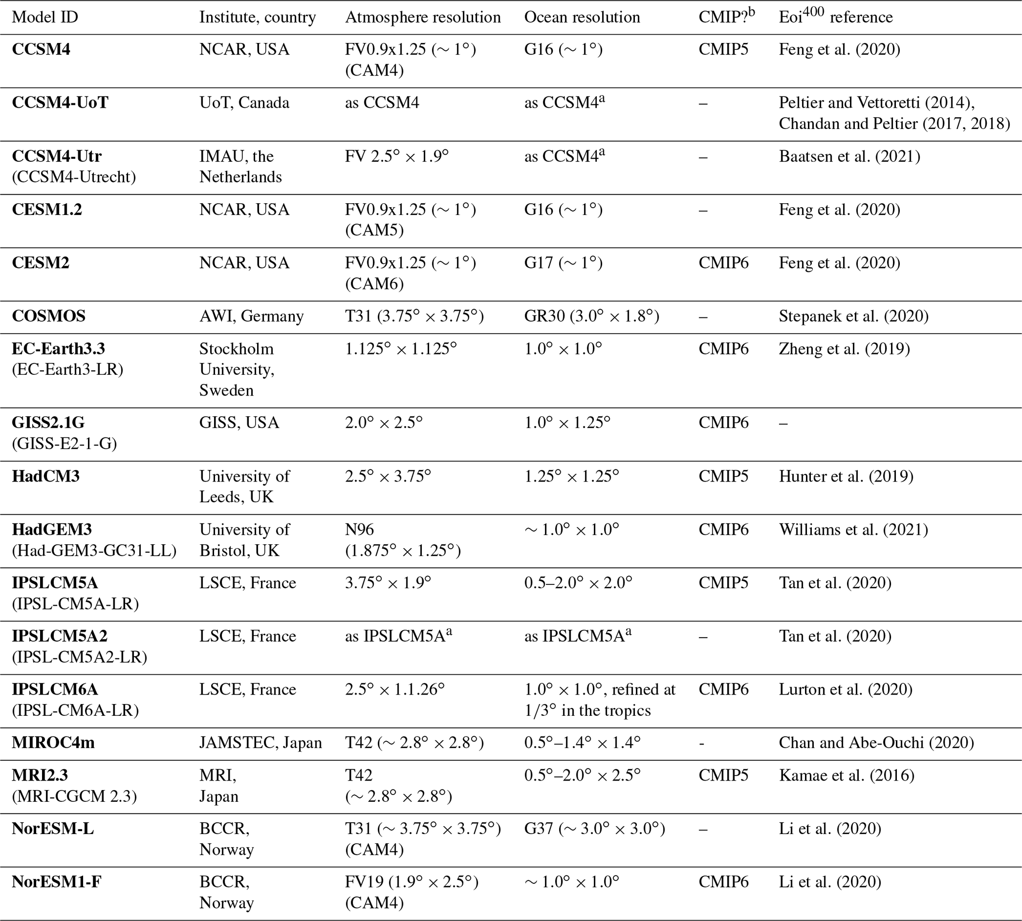
a Slight differences; check Haywood et al. (2020) for details.
b Models that contributed to the Coupled Model Intercomparison Project (CMIP) phase 5 or 6.
2.2 Analysis methods
2.2.1 Niño indices
The Niño 3.4 index, defined as the monthly SST anomaly in the Niño 3.4 region in the equatorial Pacific, is most commonly used in present-day ENSO analysis. It can be used to determine the amplitude and period of ENSO variability. The Niño 3.4 region is used since it shows the largest correlation with SST variability in the whole tropical Pacific. However, the question remains as to whether this is also true for the mid-Pliocene ENSO.
Figure 1 shows the standard deviation (SD) of the SST anomalies in the tropical Pacific for (a) the pre-industrial E280 ensemble mean and (b) the mid-Pliocene Eoi400 ensemble mean. Indicated in the plot are the four commonly used regions to study ENSO variability: the Niño 4, Niño 3.4, Niño 3 and Niño 1+2 regions. The magnitude of SST variability decreases in the mid-Pliocene equatorial Pacific, but it seems that the region with the largest ENSO-related variability keeps its position.
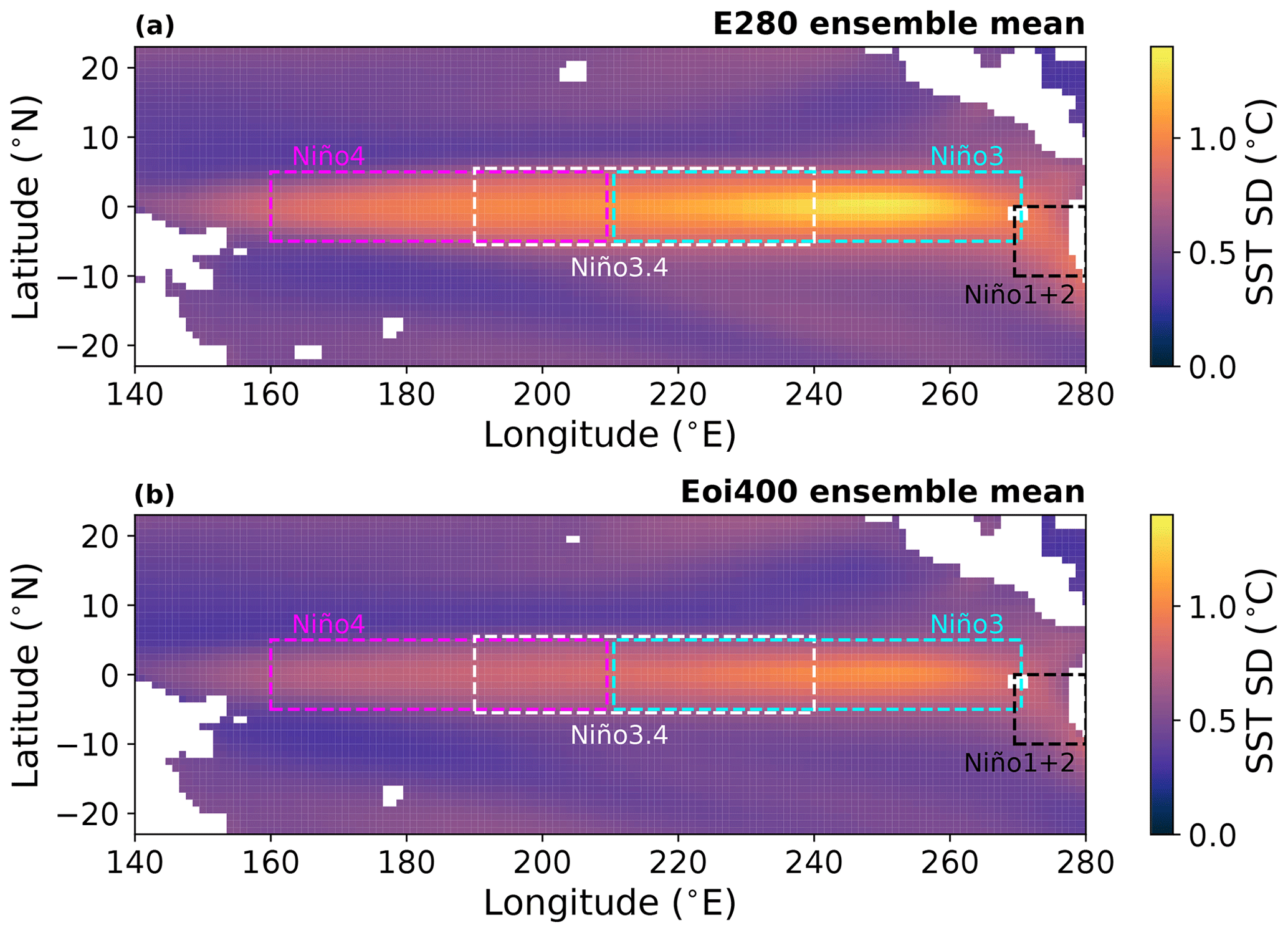
Figure 1The ensemble mean standard deviation (SD) of SST anomalies in the tropical Pacific. Results for (a) pre-industrial E280 and (b) mid-Pliocene Eoi400 simulations. Boxes drawn are the different Niño regions.
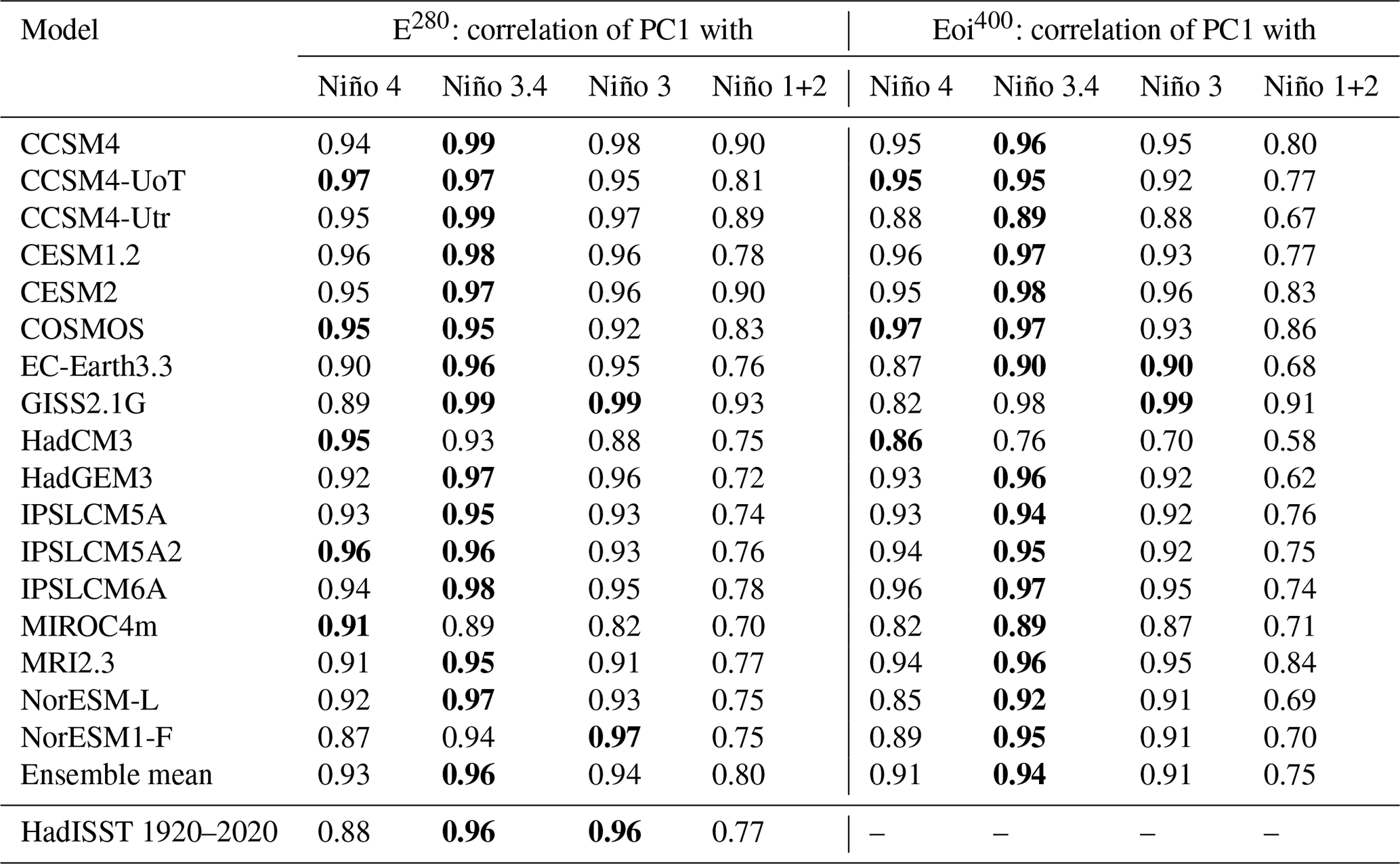
To determine the SST anomaly pattern with the largest variance, we perform principal component analysis (PCA) on the detrended monthly SST anomalies. As the climatology is subtracted, we expect the leading principal component (PC1) in the tropical Pacific to capture ENSO variability. We correlate the PC1 with the four different Niño indices to check which region is representative for ENSO variability, both in the pre-industrial simulations and in the mid-Pliocene. The results per model are presented in Table 2.
In the pre-industrial simulations, 14 of the 17 models show the largest correlation in the Niño 3.4 region. The ensemble mean shows the largest correlation for the Niño 3.4 index and the results agree well with data obtained from 1920–2020 HadISST observations (Rayner et al., 2003). Of the mid-Pliocene simulations, 15 of the 17 models show the largest correlation with the Niño 3.4 index. The mid-Pliocene ensemble mean clearly shows the largest correlation in the Niño 3.4 region. Henceforth, we will be using the Niño 3.4 index to quantify ENSO variability. Furthermore, some of the analyses performed in this study have also been repeated with the Niño 3 index instead of the Niño 3.4 index, resulting in the same conclusions.
Table 2Correlation coefficient of the first principal component (PC1) of SSTs in the tropical Pacific to the different Niño indices. The largest correlation coefficient for each model is shown in bold text.
2.2.2 Quantifying ENSO variability
In order to quantify ENSO variability within the PlioMIP2 ensemble, we look at four main features of ENSO: (1) amplitude, (2) period, (3) spatial structure and (4) El Niño flavour (see below for explanation and specific definitions used). To compute the amplitude and period we use the Niño 3.4 index. Anomalies are taken with respect to a mean seasonal cycle computed on the full 100 years of data that are available. No running mean is applied. Before any analysis, linear trends are removed from the Niño 3.4 time series. The analysis methods used here are similar to those in the analysis of ENSO in the PlioMIP1 ensemble by Brierley (2015). Results for individual models are included in the Supplement.
We assess the properties of ENSO variability using the second, third and fourth statistical moments of the Niño 3.4 index, namely the standard deviation (SD), skewness and kurtosis. The first moment, the mean, is zero by definition. The ENSO amplitude is defined as the SD of the Niño 3.4 time series. Furthermore, the skewness and kurtosis of the Niño 3.4 index are computed (following the Fischer–Pearson definition; Zwillinger and Kokoska, 2000). Both are normalized on the variance, and a factor of 3.0 is subtracted from the kurtosis to give 0.0 kurtosis for a normal distribution. Positive or negative skewness provides information on whether there are more El Niño or more La Niña events, respectively. Positive kurtosis indicates that there are more values around the mean and the SD is mainly determined by extreme values, while negative kurtosis implies a more uniform distribution of values. The kurtosis thus provides information on the relative occurrence of extreme events (i.e. El Niño and La Niña events). The variation of the Niño 3.4 SD has been investigated using 500 years of data from CESM2 and MIROC4m and was found to not be large enough to impact the conclusions of the ensemble. Results of this are included in the Supplement.
To investigate the ENSO period(s), we perform a spectral analysis of the Niño 3.4 index. Before the power spectra are computed, the indices are normalized with their SD to obtain time series with zero mean and unit SD. It was chosen to use the multi-taper spectral method as explained by Ghil et al. (2002), with three tapers and a bandwidth parameter of two. This spectral method is preferred over the classic periodogram because of its statistical robustness and reduction of spectral leakage. All spectra are scaled with respect to their respective sum. We assess the significance of spectral peaks by performing a red noise test on each time series. The 90 %, 95 % and 99 % confidence levels are determined using a first-order autoregressive (AR(1)) model with 10 000 Monte Carlo-generated surrogates.
To quantify a change in ENSO period in the mid-Pliocene from the pre-industrial, we consider two measures: (1) the ensemble mean power spectra and (2) the periods of the ensemble sum of peaks that are above the 90 %, 95 % and 99 % confidence levels. The mean power spectrum gives information on what happens to the spectral power in the mid-Pliocene. Note that the mean is taken per frequency bin to create the mean spectrum for the Eoi400 and E280 runs. However, a mean spectrum does not contain any information on the significance of the spectral peaks. For this reason, we introduce a procedure where we count all the spectral peaks above the 90 %, 95 % and 99 % confidence levels in the 1.5–10-year period per simulation. The periods of these significant peaks are then binned for the whole ensemble. This histogram of the significant peaks provides information on the period or period range that represents the most ENSO-related activity. The method has been tested for robustness by repeating the procedure using five instead of three tapers, using a bandwidth parameter of four instead of two, using the classic periodogram (fast Fourier transform) instead of the multi-taper method and using the Niño 3 instead of the Niño 3.4 index. The conclusions are found to be independent of these different settings. A summary of these results is included in the Supplement.
We use principal component analysis (PCA) on the monthly SST anomalies to investigate changes in the spatial structure of ENSO. The first empirical orthogonal function (EOF) is determined in the tropical Pacific (defined as 23∘ S–23∘ N and 140–280∘ E). We follow the methodology of Power et al. (2013) in performing EOF analysis and normalizing the EOF with the spatial SD in order to remove the ENSO amplitude signal, as Brierley (2015) did for the PlioMIP1 ensemble. As the climatology and trend are removed, we expect the first EOF in the tropical Pacific to correlate with ENSO variability and not with the seasonal cycle. The spatial EOF pattern and the percentage of variance explanation will be compared for both simulations, to assess to which degree ENSO variability differs.
We can distinguish between two El Niño “flavours”, being (1) the cold tongue or eastern Pacific El Niño and (2) the warm pool or central Pacific El Niño (also known as El Niño Modoki, Ashok and Yamagata, 2009; Yeh et al., 2009). These types are distinguishable based on the region of their largest ENSO amplitude (hence the naming). Here we use the methodology proposed by Ren and Jin (2011), using two new indices for the cold tongue (NCT) and warm pool (NWP) El Niño, combining the Niño 3 (N3) and Niño 4 (N4) indices:
where if N3N4>0 and α=0 otherwise. We will quantify whether there is a change in El Niño flavour in the mid-Pliocene by computing and comparing the SD of the NCT and NWP indices.
Lastly, we will look at the tropical Pacific mean state, specifically the zonal SST gradient in the equatorial Pacific Ocean, to find explanations for a change in ENSO behaviour. For this, we compute the annual mean SSTs in the tropical Pacific Ocean (23∘ S–23∘ N and 140–280∘ E) from the 100-year monthly data for each model and simulation. We define the zonal SST gradient as the SST difference between the warm pool region in the equatorial western Pacific Ocean (5∘ S–5∘ N, 150–170∘ E) and the cold tongue region in the equatorial eastern Pacific Ocean (5∘ S–5∘ N, 240–260∘ E). Both the tropical Pacific as well as the warm pool and cold tongue region bounds are indicated in Fig. 7, for reference. Furthermore, to assess whether the mean state of the mid-Pliocene becomes more El Niño-like, we spatially correlate the annual mean SST change (Eoi400–E280) to the pre-industrial (E280) pattern of the leading EOF.
2.2.3 Comparison with observations
We compare pre-industrial simulation results to those obtained via HadISST observational data, taken from 1920–2020 (Rayner et al., 2003, latest data available through https://www.metoffice.gov.uk/hadobs/hadisst/data/download.html, last access: 11 May 2021). The observational data can be used to assess how well individual models as well as the pre-industrial ensemble mean perform with respect to historical ENSO records. Note that there will be impacts of anthropogenic forcing such as greenhouse gas emissions in the HadISST observational data that will not be present in the pre-industrial simulation results.
The mid-Pliocene mean climate simulation results will be compared with reconstructed SST proxies by Foley and Dowsett (2019) and McClymont et al. (2020). These reconstructions resemble the 30 000 years around the KM5c interglacial in the mid-Pliocene that the Eoi400 simulations are designed to represent. The Foley and Dowsett (2019) data, part of PRISM4, are a collection of alkenone palaeo-thermometry and U SST proxies. The McClymont et al. (2020) data are a combination of U reconstructions using a BAYSPLINE calibration and foraminifera SST reconstructions (https://doi.org/10.1594/PANGAEA.911847). Together these proxies represent eight SST values from six different locations in the tropical Pacific.
3.1 ENSO variability
3.1.1 Statistical moments
Figure 2 shows the SD, skewness and kurtosis for all models with respect to their pre-industrial values. The ensemble mean is also shown in the plots, and the HadISST observational data are included as reference. Individual Niño 3.4 index time series for all ensemble members are included in Fig. S1 in the Supplement.
Figure 2a shows a clear reduction of the Niño 3.4 SD in the Eoi400 ensemble mean compared to the E280 ensemble mean, with 15 out of 17 individual models agreeing. The mid-Pliocene ensemble mean shows a 24 % reduction in ENSO amplitude (compared to 20 % in PlioMIP1, Brierley, 2015), with a standard deviation of ±18 %. The spread of the individual values is large; the difference between the smallest and largest SD is around 1.2 ∘C for both the pre-industrial and mid-Pliocene simulations. Still, the ensemble mean pre-industrial value is close to the HadISST observations (0.91±0.28 ∘C and 0.77 ∘C, respectively). Notable individual models are COSMOS for having large SD in both runs and CCSM4-Utr for showing the largest absolute decrease in SD. The models showing almost no difference between E280 and Eoi400 are COSMOS, GISS2.1G and MRI2.3. The same model version of MRI was included in the PlioMIP1 ensemble, where it also showed no change (Brierley, 2015).
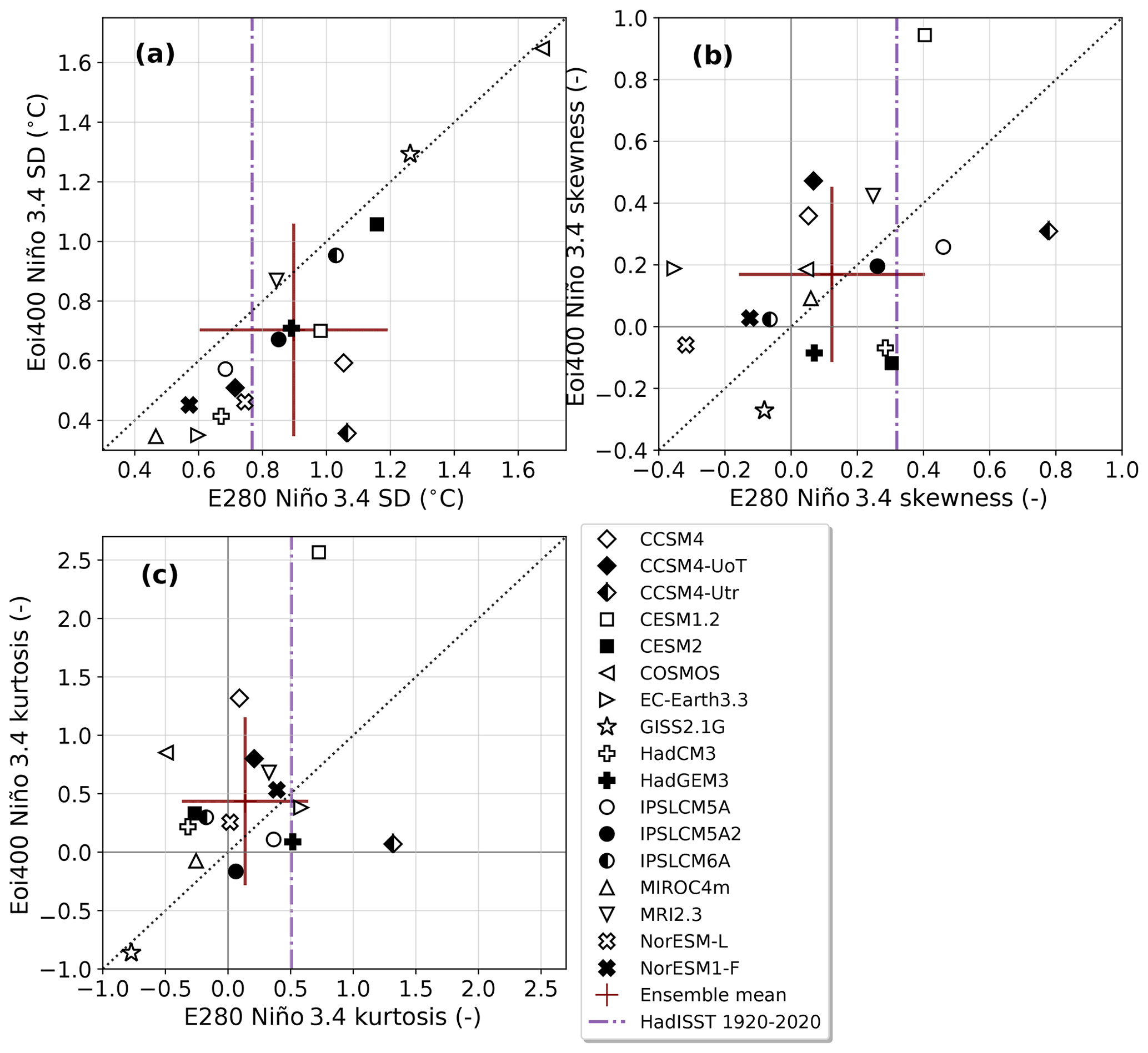
Figure 2Niño 3.4 moments for the E280 and Eoi400 runs: (a) standard deviation (SD), (b) skewness and (c) kurtosis for all models. Ensemble mean is indicated as a cross; the width and height indicate ensemble standard deviation. A dotted–dashed vertical line indicates moments from the HadISST Niño 3.4 index.
A less coherent pattern arises from the skewness of the Niño 3.4 index, shown in Fig. 2b. Again, the spread of the values is large. Most individual models (14 out of 17), as well as the ensemble mean, show a smaller skewness in the pre-industrial compared to the HadISST observations. The ensemble mean shows no significant change of the skewness in the mid-Pliocene simulations. Around half of the models (9 out of 17) show a positive skewness in both simulations, indicating generally more El Niño than La Niña events. However, the individual models do not show agreement on what happens to the skewness in the Eoi400 runs, compared to the E280 reference. GISS2.1G shows the most negative skewness in the mid-Pliocene. Both NorESM-L and EC-Earth3.3 show the most negative skewness in the pre-industrial. Notable again is CCSM4-Utr for having the largest skewness in the pre-industrial and the biggest absolute decrease in the mid-Pliocene. CESM1.2 shows the opposite behaviour with the largest increase in the skewness in the mid-Pliocene, although the pre-industrial result shows a good agreement with the HadISST data.
The kurtosis of the Niño 3.4 index is shown in Fig. 2c. The pre-industrial ensemble mean kurtosis is close to zero, which does not agree with results from the HadISST observations (albeit within standard deviation range), which show a positive kurtosis. The ensemble mean shows an increase in kurtosis in the mid-Pliocene simulations, with 11 out of 17 individual models agreeing. This indicates that the distribution becomes more “heavy-tailed”, implying that there is more activity around the mean (neutral state) and the variance is mainly determined by some extreme tail values (i.e. “extreme” El Niño or La Niña events). The notable deviations from the ensemble are GISS2.1G (large negative kurtosis in both runs), CCSM4-Utr (largest decrease) and CESM1.2 (largest increase).
3.1.2 Spectral analysis
We investigate the ENSO period by looking at the Niño 3.4 power spectra. The power spectra for all the individual simulations are shown in Fig. S2, including the HadISST spectrum. We find that 12 out of the 17 models show an increase in the period of maximum spectral power in the mid-Pliocene, compared to the pre-industrial. However, ENSO does not have one isolated period in the power spectrum. While there are models that show peaks in spectral power in the mid-Pliocene at higher periods than in their pre-industrial counterparts, in many cases these spectral peaks do not exceed the threshold for statistical significance. Therefore, we only consider the ensemble mean power spectrum as well as the histogram of significant spectral peaks here.
The ensemble mean power spectra are shown in Fig. 3. The HadISST spectrum is also included. The shading represents the second-to-smallest and second-to-largest power value per frequency. The pre-industrial spectrum resembles the HadISST spectrum, except for a less clear separation of the spectral peaks. The pre-industrial mean spectrum shows the largest power in the 3–7-year period, which is generally associated with ENSO. The mid-Pliocene mean spectrum shows a peak at a period of 5 years. The clearest change in the mid-Pliocene is the reduction of power in the 3–4-year period. However, the range in modelled values is large for both simulations, and the individual power spectra show a lot of differences in power and peak locations (see Fig. S2). Some of the models show little difference between the pre-industrial and mid-Pliocene simulations (for example CCSM4). Many show a decrease in spectral intensity in the mid-Pliocene. However, GISS2.1G and MRI2.3 also show significant peaks (>99 % CI) in the mid-Pliocene simulation that are not present in the pre-industrial reference. The clear shift to longer periods or lower frequencies found in the PlioMIP1 ensemble mean spectrum is not reproduced by the PlioMIP2 ensemble mean (Brierley, 2015).
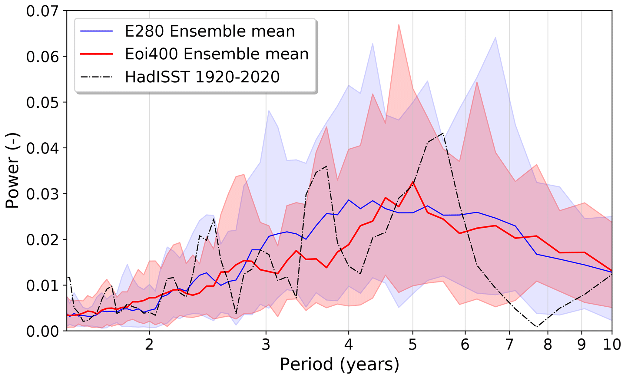
Figure 3Ensemble mean Niño 3.4 power spectra for the pre-industrial E280 (blue) and mid-Pliocene Eoi400 (red) runs. For reference, the HadISST observational Niño 3.4 spectrum is included (dotted–dashed line). Shading represents a range of modelled values, specifically the second-to-smallest and second-to-largest values.
A way to assess the change in ENSO period in the mid-Pliocene is through counting the significant peaks in the spectra, as explained in Sect. 2.2. Figure 4 shows (a) a histogram of the number of peaks that are above a certain (90 %, 95 % and 99 %) confidence level per period bin and (b) the difference between the mid-Pliocene and pre-industrial. It can be seen from Fig. 4a that the majority of the significant peaks in the pre-industrial are found in the 2–5-year period, with a clear maximum around the 3–4-year period. The total number of spectral peaks that can be called significant decreases in the mid-Pliocene for all the confidence levels. The number of peaks that are above the 99 % confidence level reduces by one-third.
The change in number of significant peaks is shown in Fig. 4b. It clearly shows the decrease in the number of peaks for all the confidence levels, mainly in the 2–5-year period. The reduction is strongest in the 3–4-year period. In the 1.5–2-year period, there is a slight increase in the number of peaks above the 90 % and 95 % confidence levels. The change in number of peaks mainly shows that the spectral power in the 3–4-year El Niño period significantly decreases and that this power does not shift to different periods.
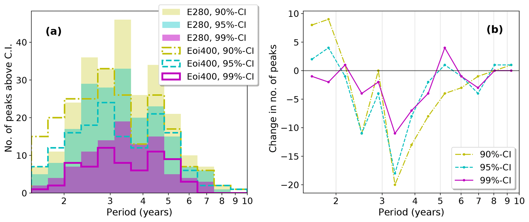
Figure 4Histogram of the number of spectral peaks that are above the 90 %, 95 % and 99 % confidence levels, binned in the 1.5–10-year period range. The number of peaks are taken from the multitaper spectra of the Niño 3.4 index for (a) pre-industrial E280 and mid-Pliocene Eoi400 runs and (b) the difference between the two.
3.1.3 Spatial structure
To study the changes in spatial structure of ENSO, we compute the EOFs of the tropical Pacific SST anomalies. The first EOFs for all the individual simulations are shown in Fig. S3. The EOFs are defined to be positive in the Niño 3.4 region. The percentage of the variance that is explained by the first EOF is also computed and shown in the bottom left of the plots.
To compare the mid-Pliocene to the pre-industrial EOFs, the ensemble means are shown in Fig. 5b–d, with the first EOF of the HadISST anomalies in 1920–2020 also included in (a). The stippling is included in regions where less than 12 out of 17 (∼70 %) models agree on the sign of the EOF. Figure 5b shows an excessive westward extension of the ENSO-related SST variability, when compared to the observational result in Fig. 5a, which is a known model bias (Jiang et al., 2021). It can be seen from Fig. 5b and c that the spatial structure looks qualitatively the same in both simulations. Also, the majority of the individual models agree with the ensemble mean pattern, indicated by the spread of the stippling. The majority of the individual models show little change, with only CCSM4-Utr, HadCM3 and MIROC4m showing spatial differences (see also Fig. S3). The percentage of variance in the tropical Pacific, which the first EOF explains, decreases from 50 % in the pre-industrial to 42 % in the mid-Pliocene within the ensemble mean. In total 14 out of 17 models agree with this decrease, with only MRI2.3 showing a slight increase in the mid-Pliocene run and COSMOS and GISS2.1G showing no change. The percentage of variance explained is very similar in the pre-industrial ensemble mean and the HadISST result.
The difference between the two ensemble mean EOFs is shown in Fig. 5d and shows a decrease in the central equatorial Pacific region. This is in agreement with the ensemble mean reduction in ENSO amplitude (or Niño 3.4 SD). The EOF difference shows an increase in the areas slightly to the north and south of this region. This suggests that there is a shift of the El Niño warmth expanding further across the tropical Pacific. This is also concluded in the PlioMIP1 ensemble, where the spatial pattern of the EOF difference looks qualitatively very similar (Brierley, 2015). Accompanying this meridional expansion of the warmth of an El Niño event is the southward migration of the South Pacific Convergence Zone (SPCZ), as was also shown by Pontes et al. (2020). It can be seen from the stippling that the majority of the models agree with a decrease in the EOF signal in the Niño 3.4 region. The rest of the tropical Pacific shows large areas with stippling, indicating that there is a lot of model disagreement on the sign of the change in EOF.
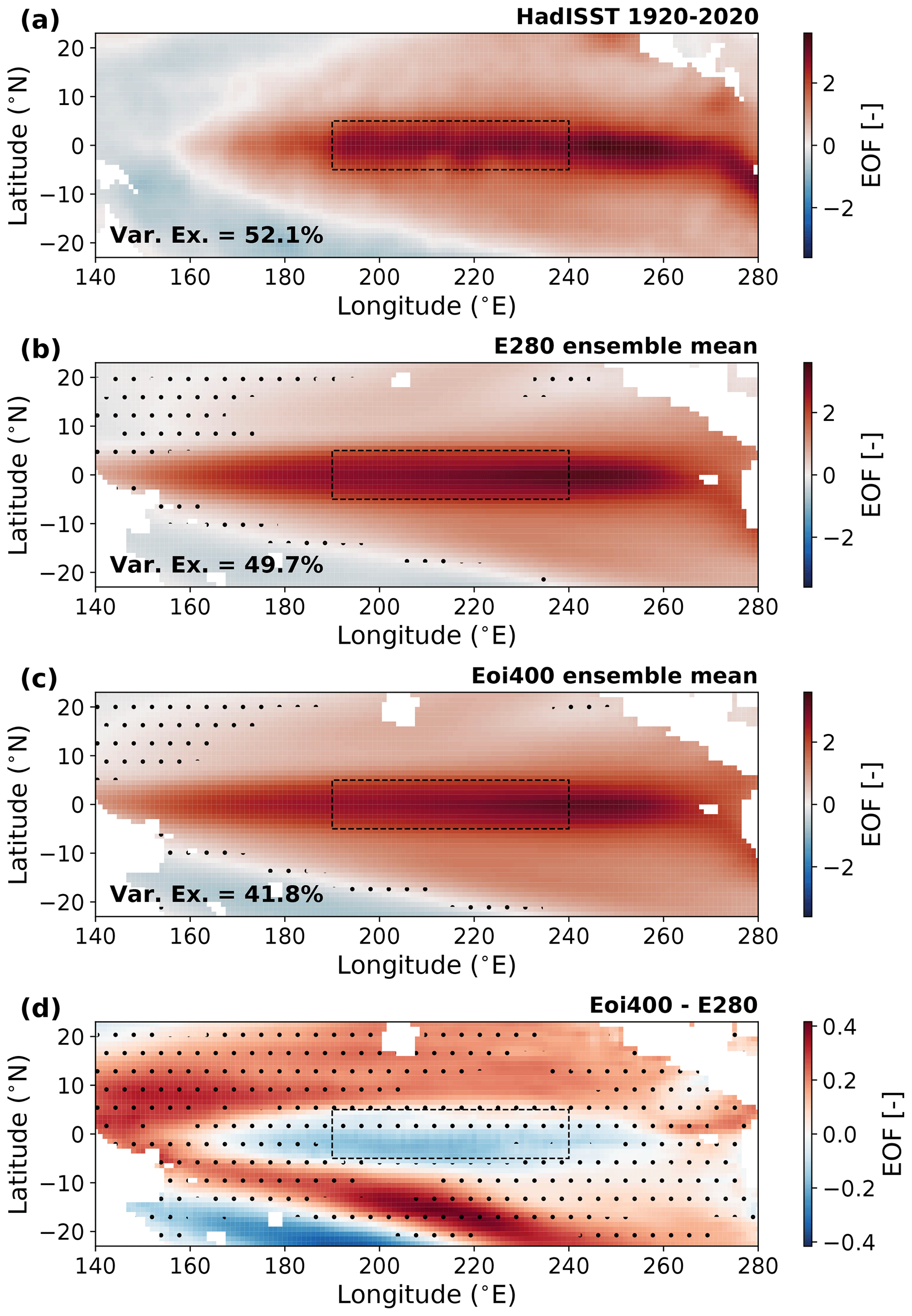
Figure 5The ensemble mean empirical orthogonal function (EOF) computed for the tropical Pacific (region shown). Ensemble mean percentage that explains the variability in the region is shown in the bottom left. Results for (a) HadISST 1920–2020 observations, (b) E280, (c) Eoi400 and (d) difference. Stippling is included if less than 12 out of 17 (∼70 %) models agree with the sign of the EOF (difference). Dashed region indicates the Niño 3.4 region, for reference.
The correlation coefficient of the leading principal component with the different Niño indices is shown in Table 2. As was concluded before, the majority of the models have the largest correlation in the Niño 3.4 region, both in the E280 as well as in the Eoi400 simulations. This result agrees with the EOF pattern results showing that the area in the tropical Pacific with the largest ENSO variability is not significantly different in the mid-Pliocene.
3.1.4 El Niño flavour
A change in El Niño “flavour” in the pre-industrial and mid-Pliocene simulations will be investigated using the methodology of Ren and Jin (2011). The amplitude of the cold tongue or eastern Pacific El Niño is defined as the standard deviation (SD) of the NCT index. Likewise, for the warm pool or central Pacific El Niño the SD of the NWP index is used. The change in magnitude of both amplitudes follows the changes in the Niño 3.4 SD results. We are interested in the difference in the ratio between the two types. The ratio of the warm pool El Niño amplitude to the cold tongue El Niño amplitude is shown in Fig. 6. For the majority of the models (13 out of 17), the ratio is smaller than 1 in both of the simulations, implying there are generally more cold tongue El Niño events. This is in agreement with the result from the HadISST observations, although the HadISST ratio is smaller than most of the model results. The ensemble mean shows no change in the ratio of warm pool to cold tongue El Niño events, and most individual models also show little change. Notable is HadCM3 for showing a majority and large relative increase in the number of warm pool El Niño events in the mid-Pliocene (very similar results to in PlioMIP1; see Brierley, 2015), and NorESM1-F and GISS2.1G for showing a small relative amount of warm pool El Niño events in both simulations. The PlioMIP2 results are somewhat similar to results from CMIP5 and CMIP6 future scenarios, which show a large model spread and no clear shift in El Niño flavour (Freund et al., 2020).
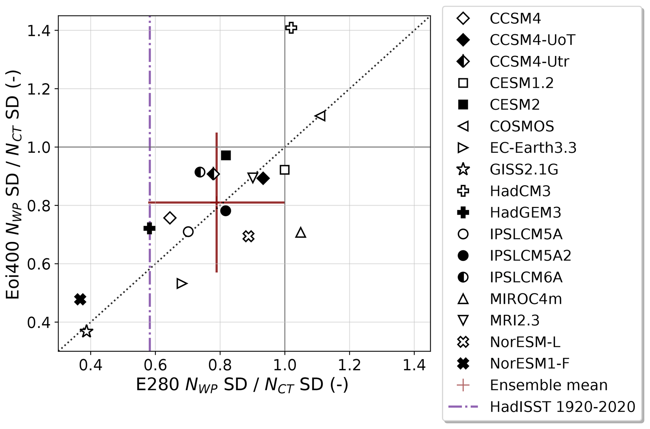
Figure 6Ratio of WP El Niño index (NWP) SD to the CT El Niño index (NCT) SD for the pre-industrial E280 and mid-Pliocene Eoi400 simulations. Ensemble mean is indicated with a cross; the width and height indicate ensemble standard deviation. A dotted–dashed vertical line indicates HadISST results.
3.2 Tropical Pacific mean climate
In this section, we will analyse changes in the tropical Pacific mean state and investigate whether this relates to the changes in ENSO variability in the mid-Pliocene simulations. We look at the tropical Pacific annual mean SSTs and specifically the zonal SST gradient along the equatorial Pacific and relate these to changes in the Niño 3.4 SD and the pre-industrial leading EOF.
3.2.1 Annual mean pattern
Figure 7 shows the annual mean SST patterns in the tropical Pacific (23∘ S–23∘ N, 140–280∘ E). The figure shows (a) results for the HadISST data from 1920–2020 (no detrending), (b–c) the pre-industrial and mid-Pliocene ensemble means, and (d) the ensemble mean differences. The circles in (b) represent the HadISST values on selected proxy locations. It can be seen that the E280 ensemble mean pattern looks qualitatively similar to the HadISST observations. Consistent with other studies using coupled GCMs (Collins et al., 2010; Coats and Karnauskas, 2017; Brown et al., 2020), the E280 means shows colder temperatures in the central and western Pacific and slightly warmer temperatures in the eastern Pacific compared to observations. The “cold bias” in the eastern Pacific can be expected since, firstly, the pre-industrial simulations are compared with historical observations and, secondly, the models have insufficient resolution to reproduce the cold conditions of coastal upwelling systems, such as the Benguela upwelling system (McClymont et al., 2020).
The Eoi400 ensemble mean is warmer but qualitatively similar to the pre-industrial result. The markers in Fig. 7c are SST proxies reconstructed by Foley and Dowsett (2019) (hereafter referred to as PRISM4) and by McClymont et al. (2020), including two U and two reconstructions (hereafter referred to as MC-UK37 and MC-Mg/Ca, respectively). There is good agreement between the PlioMIP2 ensemble mean and the PRISM4 SSTs in the eastern Pacific upwelling region. The two points in the warm pool region show slightly lower SSTs compared to the Eoi400 ensemble mean. The MC-UK37 point around 240∘ E shows a higher value compared to the ensemble mean, while the MC-Mg/Ca around 273∘ E shows a lower value.
Figure 7d shows the ensemble mean Eoi400 − E280 difference. The colour bar of the plot highlights deviations from the tropical Pacific mean SST difference ( ∘C), meaning that the red and blue areas show warmer and cooler parts with respect to the tropical Pacific mean difference, respectively. It shows specific warmer parts along the Equator and in the upwelling region in the eastern Pacific. It also shows a clear cooler part in the southern tropical Pacific, implying a shift of the SPCZ as is also seen from the change in EOF (Fig. 5d). This result agrees with findings by Pontes et al. (2020) that investigated shifts in precipitation patterns in the PlioMIP1 and PlioMIP2 ensembles.
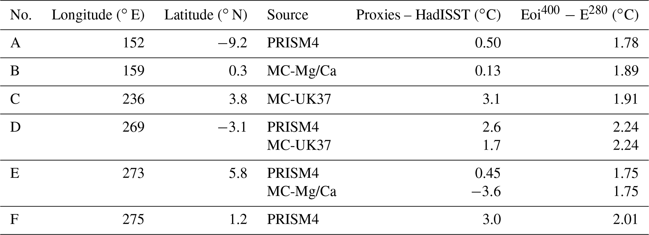
The six points A–F in Fig. 7d represent differences between proxies and HadISST; the respective eight values are presented in Table 3. Points A and B in the warm pool region show similar temperatures to those in the pre-industrial, not agreeing with the increase in temperature seen in the PlioMIP2 ensemble mean. Points C–F in the central and eastern Pacific show a better agreement with the ensemble mean difference, albeit with a range of ±1 ∘C. The only clear outlier is the MC-Mg/Ca proxy at 273∘ E at location E, indicating a significant SST decrease compared to the pre-industrial. This temperature decrease is not captured by the PlioMIP2 ensemble mean difference nor by any individual model.
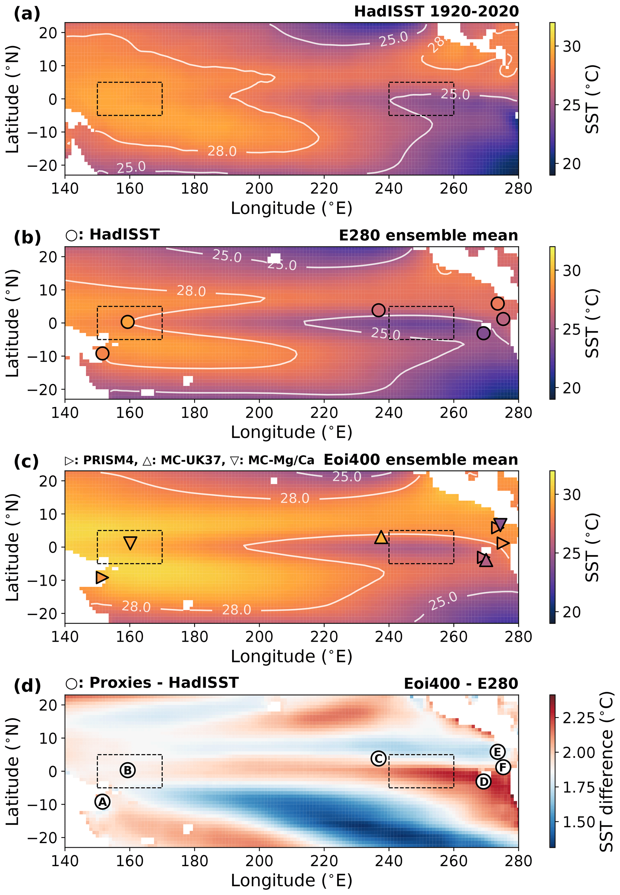
Figure 7The ensemble mean annual mean SSTs in the tropical Pacific. Results for (a) HadISST 1920–2020 observations, (b) E280, (c) Eoi400 and (d) difference between Eoi400 and E280. Dashed regions are the western Pacific warm pool and eastern Pacific cold tongue; the zonal SST gradient is computed as a difference of the mean SST in these regions. Points in (b) show the HadISST values on the proxy locations and (c) the reconstructed mid-Pliocene SST proxies from PRISM4 and MC. Points in (d) show the difference between the proxies and the HadISST data at proxy locations A–F; values are presented in Table 3.
Table 3SST difference on six different locations in the tropical Pacific, both mid-Pliocene proxy minus HadISST 1920–2020 results and the difference between Eoi400 and E280. Proxy reconstructions by Foley and Dowsett (2019) (part of PRISM4) and McClymont et al. (2020) (referred to as “MC”). Locations (with letters) are indicated in Fig. 7d.
3.2.2 Zonal SST gradient
Early observational work suggested a highly reduced zonal SST gradient in the tropical Pacific in the mid-Pliocene (Wara et al., 2005; Fedorov et al., 2013), and it has been argued that ENSO properties might be related to this mean state feature. The PlioMIP1 ensemble did not show a clear agreement on the zonal SST gradient, and it was concluded that a reduction in zonal SST gradient could not explain a reduction in ENSO variability (Brierley, 2015). Here, we will investigate whether there is any correlation between the zonal SST gradient and the change in Niño 3.4 SD in PlioMIP2.
Figure 8 shows the ensemble mean and meridional mean (5∘ S–5∘ N) SST in the Pacific Ocean. The individual model results are included in Fig. S4. The HadISST 1920–2020 result is included for reference. The shading shows the range of modelled values. The HadISST values fall within the range of pre-industrial modelled values but are on average 0.7 ∘C warmer. This “warm bias” can largely be attributed to anthropogenic warming trends that are present in the HadISST data ( ∘C in the equatorial Pacific, from 1870 to 2020) but absent in the pre-industrial simulation results. The mid-Pliocene ensemble mean follows the same zonal dependence as the pre-industrial but is consistently 2 ∘C warmer, as can be seen from the Eoi400–E280 difference. However, the model spread is large. The range of values is especially large in the eastern Pacific cold tongue region, where the modelled values range from 0 to 4 ∘C of warming.

Figure 8E280 (blue) and Eoi400 (red) ensemble mean equatorial Pacific SSTs (5∘ S–5∘ N mean), with difference shown as teal-coloured dashed line (following right vertical axis). HadISST 1920–2020 observation included as dashed–dotted line. Coloured shaded area shows the range of modelled values. Grey vertical rectangles show the region considered here to be the warm pool (left) and cold tongue (right).
We quantify the zonal SST gradient in the tropical Pacific as the SST difference between the warm pool region in the equatorial western Pacific Ocean (5∘ S–5∘ N, 150–170∘ E) and the cold tongue region in the equatorial eastern Pacific Ocean (5∘ S–5∘ N, 240–260∘ E). These regions are also indicated in Figs. 7 and 8. Figure 9a shows the zonal SST gradients for the pre-industrial and mid-Pliocene simulations. The ensemble mean shows little change in the mid-Pliocene, and a reasonable agreement with the HadISST observations. This result is in line with what is shown in Fig. 8. However, a majority of the models (13 out of 17) actually shows a slightly reduced zonal SST gradient in the mid-Pliocene simulations. The ensemble mean is very much affected by two outliers, namely MRI2.3 and COSMOS, that show a greatly increased zonal SST gradient. It should be noted that the pre-industrial simulation of MRI2.3 has its cold tongue centred around 220∘ E instead of 250∘ E, and this is the main reason for the large difference in the zonal SST gradient (see the individual model result in Fig. S4).
To investigate the relation between the zonal SST gradient and ENSO amplitude, we present a scatter plot of the change in zonal SST gradient versus the change in Niño 3.4 SD in Fig. 9b. The ensemble mean shows a ∼24 % decrease in Niño 3.4 SD despite little change in zonal SST gradient ( ∘C). The “cluster” of models around the ensemble mean does show a slightly more reduced zonal SST gradient together with a robust reduction in Niño 3.4 SD. On the one hand, CESM2 shows the largest reduction in zonal SST gradient but a small reduction in Niño 3.4 SD. On the other hand, both COSMOS and MRI2.3 show a great increase in zonal SST gradient but a similar Niño 3.4 SD, although for MRI2.3 the increase in zonal SST gradient is mainly due to the overly westward extent of the cold tongue in the MRI2.3 model discussed above. CCSM4-Utr, however, shows the largest reduction in Niño 3.4 SD despite a similar zonal SST gradient. Ultimately, there does not seem to be a strong correlation between the change in zonal SST gradient and the change in Niño 3.4 SD in the PlioMIP2 ensemble. This conclusion is consistent with a recent study by Brown et al. (2020) considering a large ensemble of CMIP5/6 and PMIP3/4 simulations, of which 10 out of the 32 models included have also contributed to the PlioMIP2. Fredriksen et al. (2020) analyse results of future scenarios with 11 CMIP6 models and link a reduced zonal SST gradient with an increase in ENSO amplitude, which would disagree with our findings. However, Beobide-Arsuaga et al. (2021) perform a similar analysis on 56 CMIP5 and CMIP6 contributions and also conclude that the relationship between ENSO amplitude change and zonal SST gradient is weak.
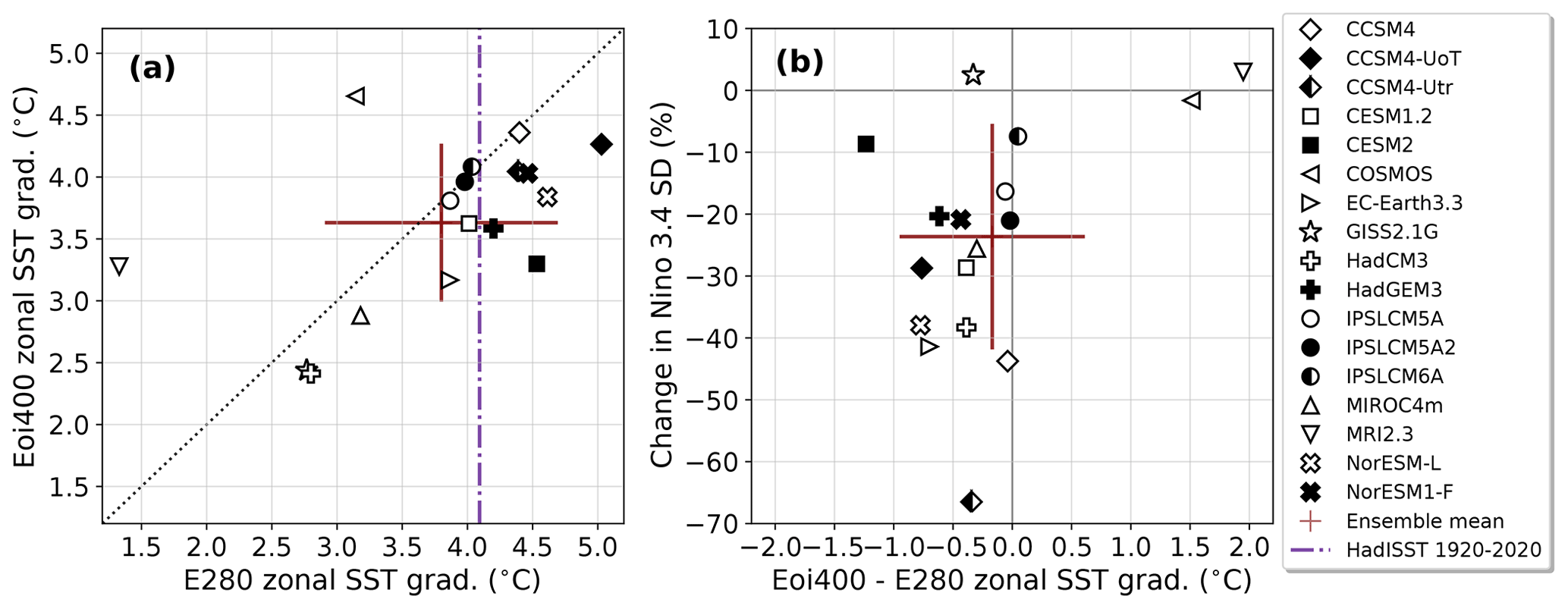
Figure 9(a) Scatter plot of E280 versus Eoi400 zonal SST gradient. Red cross represents ensemble mean; dashed–dotted line shows the HadISST 1920–2020 value. (b) Scatter plot showing the change in Niño 3.4 SD as a function of the change in zonal SST gradient in the equatorial Pacific.
3.2.3 The El Niño-like mean state
To investigate whether the mean SST pattern in the tropical Pacific is El Niño-like, we project the changes in the mean state (i.e. Eoi400 SSTs − E280 SSTs) onto the leading EOF of the pre-industrial E280 simulation for each model and perform a spatial correlation. If this correlation is positive, it implies that the mid-Pliocene mean SSTs are more similar to the pre-industrial El Niño than the pre-industrial mean SSTs. Likewise, if the correlation is negative, the mid-Pliocene mean can be said to be more similar to a La Niña. Results are shown in Fig. 10a. The ensemble mean shows no correlation of the mean state changes to either an El Niño or a La Niña, and about half of the individual models (8 out of 17) also show little correlation (between −0.3 and 0.3). Interestingly, there is a “cluster” of models (“A”: GISS2.1G, COSMOS, IPSLCM6A and CESM2) that show a clear positive correlation (El Niño-like) but little to no change in the Niño 3.4 SD. On the other side, there is cluster – albeit less clearly grouped – showing a negative correlation (La Niña-like) and the largest reduction in Niño 3.4 SD (“B”: CCSM4-Utr, EC-Earth3.3 and CCSM4). This contrasting result between CCSM4 and CESM2 was already observed by Feng et al. (2020). Taking into account all the models, there seems to be an increasing trend: the more El Niño-like, the smaller the reduction in ENSO amplitude is. A similar trend is found by Pontes et al. (2021), when considering changes in the thermocline slope in the PlioMIP2 simulations. However, we should consider here the results from the PlioMIP1 ensemble (Brierley, 2015), shown in Fig. 10b, that suggest the opposite trend. Although some of the individual models that were also a part of PlioMIP1 show very different results in PlioMIP2, the ensemble mean is actually very similar, despite the fact that different boundary conditions are used in both MIP protocols.
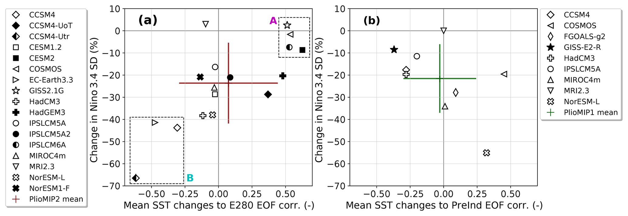
Figure 10Scatter plot of the correlation coefficient of the annual mean SST changes to the leading pre-industrial EOF in the tropical Pacific versus the change in Niño 3.4 SD. Results for (a) the PlioMIP2 ensemble as well as (b) the PlioMIP1 ensemble (Brierley, 2015). Some models were a part of both ensembles, but note that a different protocol was used in the both MIPs.
To analyse the El Niño-like mean state in a more detailed fashion, we focus on the two “clusters” that were identified in Fig. 10a. We show the cluster model-mean pattern of the annual mean SST changes and the pre-industrial E280 EOF in the tropical Pacific in Fig. 11. The first group of models is GISS2.1G, COSMOS, IPSLCM6A and CESM2 (group A, Fig. 11a–b), showing El Niño-like mean state changes and strong ENSO variability. The mean state changes show a clear warming pattern along the Equator, very much like the pre-industrial EOF pattern. The warming is also very uniform, implying no changes in the zonal SST differences compared to the pre-industrial. The second group of models is CCSM4-Utr, EC-Earth3.3 and CCSM4 (group B, Fig. 11c–d) and show La Niña-like mean state changes with a strongly reduced ENSO amplitude. The mean state changes show a relatively weaker warming along the Equator compared to the tropical Pacific mean SST changes. Large variations can be seen in the western Pacific, where the equatorial warm pool region warms the least and the subtropical regions show a higher than average warming. The mean state changes show a clear anticorrelation with the pre-industrial EOF pattern. Interestingly, this group also shows a large warming in the upwelling region along the South American Pacific coast. This implies a reduction in the zonal SST gradient between the upwelling region and the warm pool, in comparison to the pre-industrial.

Figure 11(a, c) “Cluster”-mean annual mean SST changes and (b, d) pre-industrial leading EOF in the tropical Pacific. For “A”: CESM2, COSMOS, GISS2.1G and IPSLCM6A (a, b). For “B”: CCSM4, CCSM4-Utr and EC-Earth3.3 (c, d).
We have investigated ENSO variability in the PlioMIP2 ensemble using a set of different metrics. Some results are quite robust (reduced Niño 3.4 SD, similar spatial structure), but the ensemble often shows a large spread in values. In this section, we will discuss the results in light of observations (both present-day and palaeo) and inter-model differences, and we will suggest possible physical mechanisms of a consistently reduced ENSO variability in the mid-Pliocene simulations.
4.1 Data–model comparison
4.1.1 Pre-industrial observations
We have included the results from the HadISST 1920–2020 dataset as a reference for the pre-industrial simulation results. The time range of the observational data does not cover the pre-industrial period and includes anthropogenic forcing trends (although a linear trend is removed). An argument to use the most recent data is the observational uncertainty that is present in the instrumental record, especially before 1920, as shown by Ilyas et al. (2017) using HadCRUT4 data. It was decided to use a 100-year time series, as with the PlioMIP2 data, and use the most recent data because of a higher spatial resolution. Chelton and Risien (2016) mention zonal and meridional discontinuities in the HadISST dataset, specifically in the Pacific. They advise caution for high-resolution studies but deem the data adequate for large-scale SST variability studies. Haywood et al. (2020) prefer to use the NOAA ERSST v5 dataset (Huang et al., 2017) over the HadISST data because of consistency with other observational datasets on a global scale.
The Niño 3.4 moments of the E280 simulations match reasonably well with those from the HadISST data (see Fig. 2). The ensemble mean shows a slightly higher Niño 3.4 SD (0.90) compared to the HadISST results (0.77). The PlioMIP1 ensemble mean reported a slightly lower SD (0.78, Brierley, 2015) and was compared to the Niño 3.4 SD of the ERSST data (0.69). The overestimation of the model Niño 3.4 SD compared to observational data is also reported in the CMIP5 ensemble (Kim et al., 2014). However, there is a good match with the HadISST tropical Pacific leading EOF and that of the E280 ensemble mean; both in the percentage of variance explained (both 50 %) and correlation of the Niño 3.4 index with the first PC (both 0.96). This shows that the PlioMIP2 ensemble does a reasonable job in representing pre-industrial ENSO variability.
There is a slight mismatch considering the warm pool (or Central Pacific) to cold tongue (or eastern Pacific) El Niño occurrence ratio (Fig. 6). The E280 ensemble mean shows a considerably higher ratio (0.80) compared to the HadISST ratio (0.60). The ensemble mean results do agree with a present-day model ensemble presented in Yeh et al. (2009) (approximately 0.6–0.9, although a slightly different method was used).
4.1.2 Mid-Pliocene proxies
Figure 7 shows a reasonable agreement of the annual mean SSTs with the proxy reconstructions by Foley and Dowsett (2019) and McClymont et al. (2020). The close agreement with most proxies in the eastern Pacific upwelling region is promising, as the mid-Pliocene ensemble mean shows the greatest warming in this region compared to the pre-industrial ensemble mean. One proxy around 240∘ E (point C) suggests a higher temperature than the ensemble mean. Considering the two proxy locations in the western equatorial Pacific, the proxies suggest a flat zonal SST profile, possibly indicating an El Niño-like mean state. However, the ensemble mean shows more warming in the western equatorial Pacific and shows a clear zonal SST gradient (see also Fig. 8), albeit slightly reduced compared to the pre-industrial. It should be noted here that the reconstructions by McClymont et al. (2020) are reported to have a significant cold bias, in comparison to the U reconstructions and the PlioMIP2 results. This can explain the severe underestimation in SST by the proxy at 273∘ E (at point E), in comparison to the PlioMIP2 ensemble mean. Another note regarding the McClymont et al. (2020) reconstructions is the reported error of 1.5 ∘C on their data. This is approximately the same as the range of modelled values on the proxy locations. Taking into account these uncertainties, the model differences fall within the range of the reported error around the observational differences (proxy minus HadISST) as reported in Table 3, with the exception of the 273∘ E proxy. Another comment is that some proxies are located close to coastal areas, where sharp contrasts and large spatial variations in SSTs can be present due to boundary currents and coastal upwelling systems. The PlioMIP2 models generally have insufficient resolution to reproduce upwelling systems (McClymont et al., 2020), and a significantly higher resolution (∼0.1∘) is needed to accurately resolve these (Small et al., 2014). When putting the proxies in a global perspective, there is generally a good agreement with proxies and the PlioMIP2 ensemble mean in the tropics, but discrepancies occur in the middle and higher latitudes, specifically in the Northern Hemisphere. This holds both for the PRISM4 reconstructions (Haywood et al., 2020) and for the McClymont et al. (2020) reconstructions.
The PlioMIP2 ensemble shows that it is likely that there was a slight reduction of the zonal SST gradient in the mid-Pliocene equatorial Pacific (Fig. 8), but not as large as some earlier proxy reconstructions suggested. Furthermore, the mean SST changes are not specifically El Niño-like, as the majority of the ensemble members do not show a positive correlation with the E280 leading EOF of tropical Pacific SSTs (Fig. 10). The PlioMIP2 ensemble also shows clear ENSO variability (although weaker than in the pre-industrial), agreeing with the proxy-based reconstructions by Scroxton et al. (2011), Watanabe et al. (2011) and White and Ravelo (2020). More specifically, White and Ravelo (2020) suggest that mid-Pliocene ENSO variability varied between reduced and similar to the present day, which is also captured by the PlioMIP2 ensemble. Watanabe et al. (2011), however, suggest that ENSO variability is similar to the present day, something most PlioMIP2 models do not agree with. Still, the PlioMIP2 ensemble includes four models (of which three participate in CMIP6) that show both ENSO variability similar to the present day and a mean state that is more El Niño-like (Fig. 10a).
4.2 Model differences
The PlioMIP2 ensemble shows robust signals when comparing mid-Pliocene and pre-industrial ENSO: the Eoi400 simulations show a reduced ENSO variability (15 out of 17 models, Fig. 2), a robust decrease in spectral peaks in the 3–4-year period (Fig. 4), a similar spatial structure of ENSO compared to the pre-industrial (Fig. 5 and Table 2) and a (slight) reduction of the tropical Pacific zonal SST gradient (14 out of 17 models, Fig. 9). Still, the spread of the individual model results is often large, and not all findings are unambiguous. Below we will discuss the possible causes of differences between models.
4.2.1 Models deviating from the ensemble mean
Some of the clear outliers are as follows:
-
Niño 3.4 index. COSMOS for showing by far the largest Niño 3.4 SD (∼1.7∘C) in both pre-industrial and mid-Pliocene simulations; COSMOS, GISS2.1G and MRI2.3 for showing almost unchanged Niño 3.4 SD in both simulations; CCSM4-Utr for showing the largest reduction in Niño 3.4 SD in the mid-Pliocene (−67 %); and GISS2.1G for showing a very regular Niño 3.4 index and an almost single-peaked Eoi400 power spectrum;
-
ENSO structure. CCSM4-Utr, HadCM3 and MIROC4m for showing large changes in the Eoi400 EOF pattern and COSMOS and HadCM3 for being the only models showing more warm pool to cold tongue El Niño events in both the pre-industrial and mid-Pliocene simulations;
-
Mean SSTs. COSMOS and MRI2.3 for showing a large increase in the zonal SST gradient from Eoi400 to E280 (+1.5 ∘C and +2.0 ∘C, resp.), where COSMOS shows a strong `El Niño-like' mean state whereas MRI2.3 shows no particular correlation; CESM2 for showing the largest decrease in zonal SST gradient from Eoi400 to E280 (−1.2 ∘C), as well as a clear El Niño-like mean state; and CCSM4-Utr for showing the most La Niña-like mean state changes.
MRI2.3 did not use the provided “enhanced” boundary conditions, but the “standard” version (Haywood et al., 2016b). This is the best possible realization of the mid-Pliocene conditions (such as vegetation and land ice cover) using a modern land–sea mask with closed Arctic ocean gateways. This could explain why MRI2.3 shows an unchanged Niño 3.4 index, as well as no change in the WP CT El Niño ratio. Next to this, its Eoi400 mean state changes show no particular correlation with the E280 EOF, neither in PlioMIP2 nor in MRI2.3's contribution to PlioMIP1. However, HadGEM3 also used the pre-industrial land–sea mask for its mid-Pliocene simulations (with closed Canadian Archipelago, open Bering strait, mid-Pliocene vegetation and land ice cover) and clearly shows different ENSO variability in both its simulations. The explanation for MRI2.3's large increase in zonal SST gradient is its anomalous pre-industrial equatorial Pacific zonal SSTs, showing a cold tongue around 220∘ E, disagreeing with the HadISST observations and all other ensemble members.
CCSM4-Utr started the Eoi400 spin-up with ocean temperatures obtained from PlioMIP1 results, whereas most other models used pre-industrial conditions as ocean temperature initialization (Baatsen et al., 2021). It shows one of the highest SAT differences, even though it has a very modest ECS compared to the rest of the ensemble (Haywood et al., 2020). Next to this, it shows a large increase in deep-ocean temperatures, namely 4 ∘C warmer (Baatsen et al., 2021). This is high considering the 2.8 ∘C SAT increase that the PlioMIP2 ensemble mean shows over oceans (Haywood et al., 2020). This could explain why CCSM4-Utr proves to be quite an outlier, especially showing a huge reduction in Niño 3.4 SD and the most La Niña-like mean state in the mid-Pliocene. However, also CESM1.2 and CESM2 have used a “warm” ocean initialization (Feng et al., 2020) and do not show the same extreme behaviour.
COSMOS also stands out and has one of the coarsest ocean resolutions (∼3∘) of the ensemble. NorESM-L has a similar ocean resolution, however, but usually behaves quite close to the ensemble mean. COSMOS is furthermore the only model that included a dynamic vegetation model, but it seems unlikely that this could have such a big effect on tropical Pacific variability. COSMOS is the only non-CMIP6 model that has a high ECS (4.7 ∘C), although it is not the highest of the PlioMIP2 ensemble (Haywood et al., 2020).
Other models with a high ECS are HadGEM3 (5.5 ∘C), CESM2 (5.3 ∘C) and IPSLCM6A (4.8 ∘C) and are all CMIP6 models (Haywood et al., 2020; Williams et al., 2021). Where HadGEM3 and IPSLCM6A perform reasonably close to the ensemble mean, CESM2 values are often outside of the standard deviation range around the ensemble mean. It shows a Niño 3.4 SD that is large in both the pre-industrial and the mid-Pliocene, and a change that is small compared to the ensemble mean (−9 % to −24 %). Furthermore, its mid-Pliocene mean state shows the largest reduction in zonal SSTs and the most El Niño-like mean state. A high ECS alone cannot explain this. CESM1.2 generally performs close to the ensemble mean, and differences between CESM1.2 and CESM2 include an updated atmospheric model (CAM5 to CAM6), land model, sea ice model and a new mixing scheme in the ocean model (Feng et al., 2020) that could all explain the different performance.
4.2.2 Model generation and family
PlioMIP2 includes CCSM4, CCSM4-UoT, CCSM4-Utr, CESM1.2 and CESM2 (the “CESM” family) that share a lot of similarities, especially in their ocean models. The five models show a very similar pre-industrial Niño 3.4 SD (∼0.8–1.2 ∘C), but no agreement in the mid-Pliocene Niño 3.4 SD (∼0.3–1.1 ∘C). They do show a great similarity in the ratio of WP and CT El Niño events between both simulations. However, the five models show little agreement in both the change in zonal SST gradient and the El Niño-like mean state results; CESM2 shows a strongly reduced zonal SST gradient and an El Niño-like mean state, whereas CCSM4 shows almost no change in zonal SST gradient and a more La Niña-like mean state. The results of CCSM4, CESM1.2 and CESM2 are discussed in more detail in Feng et al. (2020). They find a weakened Walker circulation and reduced upwelling in CESM1.2 and CESM2, but not in CCSM4, and this could explain the aforementioned differences.
The two NorESM models (NorESM-L and NorESM1-F) as well as the three IPSL models (IPSLCM5A, IPSLCM5A2 and IPSLCM6A) generally do show a great similarity between their results. HadCM3 and HadGEM3 both belong to the “Hadley Centre” model family but show very different results. Generally HadGEM3 performs close to both the pre-industrial and mid-Pliocene ensemble means. The HadGEM3 pre-industrial results furthermore show a great match with the HadISST observations. The HadCM3 results are overall less close to the ensemble mean. More information on the difference in large-scale features between HadCM3 and HadGEM3 can be found in Williams et al. (2021).
Brown et al. (2020) as well as Jiang et al. (2021) argue that the simulation of ENSO may be improved in CMIP6 (compared to CMIP5), especially due to improvements in the simulation of the mean state in the tropical Pacific, such as a reduced double intertropical convergence zone (ITCZ) bias and cold tongue bias. When only the results of CMIP6 models (CESM2, EC-Earth3.3, GISS2.1G, HadGEM3, IPSLCM6A, NorESM1-F) are considered, the ensemble mean results and the conclusions on mid-Pliocene ENSO variability are similar. However, the CMIP6 models do show the strongest reduction in zonal SST gradient in the mid-Pliocene (Fig. 9). Also, it is mainly the CMIP6 models that show El Niño-like mean state changes (Fig. 10), although EC-Earth3.3 exhibits a La Niña-like mean state.
4.2.3 PlioMIP2 versus PlioMIP1
In total, 7 of the 17 models that participate in PlioMIP2 also participated in PlioMIP1, namely CCSM4, COSMOS, HadCM3, IPSLCM5A, MIROC4m, MRI2.3 and NorESM-L. Some of the PlioMIP1 conclusions presented in Brierley (2015) are similar: the Niño 3.4 SD decreases (24 % (±18 %) in PlioMIP2 versus 20 % in PlioMIP1), the spatial structure of El Niño is similar and the El Niño flavour shows no robust change. However, there are also some clear differences. PlioMIP2 shows a significant reduction of the spectral power in the 3–4-year period, where PlioMIP1 mainly shows a shift of power to longer periods; the PlioMIP1 results showed a clear “low-frequency” peak in the pre-industrial around 5–6 years that seemed to shift to 7–8 years in the mid-Pliocene ensemble mean. The significance of the spectral peaks was not assessed, however. Another difference is that the PlioMIP2 models show a clear but small reduction in zonal SST gradient where PlioMIP1 shows “no preferential warming in the eastern equatorial Pacific”. An explanation for the difference between the ensemble results is that PlioMIP2 encompasses more and newer models (most CMIP6) that have a higher resolution and include the newest ocean–atmosphere models and parametrizations. Next to this, the boundary conditions of PlioMIP2 are more specifically tuned to a specific time slice in the mid-Pliocene (Dowsett et al., 2016). It should also be noted that Brierley (2015) used more than 100 years of data (up to 200 years) for analysis of some of the models, sometimes including more years of pre-industrial data than mid-Pliocene data for one model. This can impact the statistical confidence of spectral power density, particularly for the longer periods. We chose to use 100 years of data for all the simulations for the sake of consistency, as some models only had 100 years of data available. The different simulation protocol and ensemble composition means that differences between PlioMIP1 and PlioMIP2 can be expected. However, the similarities between both ensembles make the reduction of the ENSO amplitude in the mid-Pliocene more robust.
4.3 Robustness of ENSO amplitude and significant-peak analysis
Previous studies from Wittenberg (2009) and Tindall et al. (2016) show that ENSO variability can exhibit significant changes on the interdecadal and centennial scale. While a time-series length of 100 years as used here is clearly sufficient to study properties such as amplitude and spectra of ENSO on its typical interannual timescales, the presence of centennial-scale modulations on ENSO properties could imply that the choice of the 100-year segment affects our conclusions on interannual variability differences between pre-industrial and mid-Pliocene. In order to address this issue, we repeated the calculation of the ENSO amplitude with 500 years of data. For this we used data of two PlioMIP2 models, MIROC4m and CESM2. The results are included in the Supplement. There are clear variations in the ENSO amplitude on centennial timescales. The change in Niño 3.4 SD varies around ±9 % and ±4 % of the value when using 500 years of data for CESM2 and MIROC4m, respectively. However, these variations are not large enough to change the conclusion regarding the clear reduction of the ENSO amplitude in the PlioMIP2 ensemble. These results are in accordance with the findings by Tindall et al. (2016), who use 2500 model years of HadCM3 simulations. When interpreting the ±9 % variation as an error margin on the change in Niño 3.4 SD, only three out of the seven models that contributed to both PlioMIP1 and PlioMIP2 show a similar result in the both MIPs, namely IPSLCM5A, MIROC4m and MRI2.3. The other models (CCSM4, COSMOS, HadCM3 and NorESM-L) show no overlap in their PlioMIP1 and PlioMIP2 values. These discrepancies cannot be explained by centennial-scale variations of ENSO amplitude and are thus likely caused by the differences in the MIP protocols.
Next to this, the spectral “peak-counting” method is tested for robustness by repeating the procedure using different spectral settings and the Niño 3 instead of Niño 3.4 index. The conclusions are found to be independent of these different settings. A summary of these results is included in the Supplement. In conclusion, both the reduction of ENSO amplitude as well as the changes in significant spectral peaks in the PlioMIP2 ensemble are robust.
4.4 Physical mechanisms
What the PlioMIP2 simulations have in common is the use of identical forcing and (nearly) identical boundary conditions. The changes in ENSO response and mean state in the mid-Pliocene should therefore be a response to the CO2 forcing and the PRISM4 boundary conditions. Brierley (2015) discusses the impact of the PRISM3 boundary conditions on ENSO and cannot find a clear explanation when considering geography. Differences in boundary conditions from PlioMIP1 to PlioMIP2 mainly include changes to lakes, soils and vegetation, land ice cover, and Arctic gateways such as the Bering strait and Canadian archipelago (Dowsett et al., 2016; Haywood et al., 2016b). We do not expect these differences to directly impact ENSO properties. Brierley and Fedorov (2016) find that the closing of the Bering strait affects ENSO properties but mention it is hard to estimate the statistical significance of these changes. Other changes to the land–sea mask include the shoaling of the Sahul and Sunda shelves. This can affect the Indonesian throughflow, which can affect ENSO properties as shown by Jochum et al. (2009) as well as Brierley and Fedorov (2016). We did not investigate the changes in the Indonesian throughflow in the PlioMIP2 ensemble in this study.
Proxy records suggest the mid-Pliocene mean state sustained El Niño-like conditions (Fedorov et al., 2006; Wara et al., 2005) or at least a weak zonal SST gradient (Fedorov et al., 2013). Manucharyan and Fedorov (2014) state that the weak zonal SST gradient was less favourable for ENSO occurrence. The PlioMIP2 results do show a reduced zonal SST gradient, but only slightly, together with a reduced ENSO amplitude. However, a consistent relationship between the two is absent, as can be seen in Fig. 9. Brown et al. (2020) investigate the relationship between zonal SST gradient and Niño 3.4 SD for PMIP3/4 simulations of the mid-Holocene, last glacial maximum and last interglacial, as well as 1 % CO2 and abrupt 4× CO2 experiments, and also find no clear relationship. Hu et al. (2013) suggest the relationship between zonal SST gradient and ENSO amplitude might be nonlinear.
Feedback analysis shows that reduction of ENSO variability in the mid-Holocene is likely due to the increase in the negative feedback (mean current thermal advection, An and Bong, 2018), the reduction of major positive feedback processes (thermocline, zonal advection and Ekman feedbacks, Chen et al., 2019) or an enhanced seasonal cycle (Iwakiri and Watanabe, 2019). However, PlioMIP1 (Brierley, 2015) as well as PMIP3 and PMIP4 models (Brown et al., 2020) do not show any consistent relationship between changes in the seasonal amplitude and changes in ENSO variability. More recently it has been suggested that the mid-Pliocene saw a generally deeper thermocline and thus a weaker thermocline feedback (White and Ravelo, 2020). Brown et al. (2020) acknowledge that the changes in feedback processes in PMIP3/4 simulations are model-dependent. They also point out that ENSO feedbacks are still inaccurately simulated in most current GCMs (Bayr et al., 2019; Bellenger et al., 2014; Kim et al., 2014; Kim and Jin, 2011).
Recent work by Pontes et al. (2021), analysing both PlioMIP1 and PlioMIP2 results, find that models with a steeper thermocline (deemed La Niña-like in that paper) are related to major ENSO reduction, while a flatter thermocline (El Niño-like) is associated with a similar ENSO amplitude compared to the pre-industrial. This finding is in agreement with the results we find on ENSO amplitude and the El Niño-like mean state (Fig. 10), although a different methodology is used. Pontes et al. (2021) furthermore find that a combination of off-equatorial mean state changes in the mid-Pliocene is not favourable for ENSO. They find a northward displacement of the ITCZ, increased south-eastern trade winds in the western Pacific and an intensified South Pacific Subtropical High in the mid-Pliocene simulations, all associated with suppression of ENSO variability.
The Pliocene Model Intercomparison Project phase 2 (PlioMIP2) coordinated 17 global coupled climate models to simulate the mid-Pliocene and pre-industrial climate. In this work, we have studied the changes in ENSO variability in the mid-Pliocene using the PlioMIP2 ensemble and related those to SST changes in the tropical Pacific mean climate. Even with (nearly) identical forcing and geographical boundaries, the PlioMIP2 ensemble includes a range of model resolutions, parametrizations and initializations, all which contribute to a considerable model spread in the PlioMIP2 ensemble.
The PlioMIP2 ensemble shows a robust decrease in ENSO amplitude. The Niño 3.4 SD decreases for 15 of the 17 models with an ensemble mean decrease of 24 %, compared to 20 % in PlioMIP1 (Brierley, 2015). Changes in Niño 3.4 skewness and kurtosis are less coherent. Spectral analysis shows a clear reduction of spectral power in the 3–4-year period in the mid-Pliocene. Furthermore, the total number of spectral peaks that are above the 99 % confidence level decreases by one-third in the PlioMIP2 ensemble. The shift towards longer periods that is suggested by the PlioMIP1 models does not occur in PlioMIP2. The mid-Pliocene ENSO is similar in spatial structure in comparison to the pre-industrial. EOF analysis shows that the percentage of variance explained by the first EOF decreases from 50 % to 42 % and suggests that El Niño warmth expands meridionally across the tropical Pacific. Correlation with the principal component time series shows that the Niño 3.4 index best captures the ENSO-related variability in the Pacific in both the pre-industrial and mid-Pliocene, also suggesting a similar spatial structure. Analysis of El Niño flavour suggests no particular change in the mid-Pliocene, although the model spread is large.
The tropical Pacific mean SSTs show a clear warming in the eastern Pacific upwelling region, in agreement with proxy data. The PlioMIP2 models do not show a unanimous weakening of the mean zonal SST gradient, with an ensemble mean change of ∘C. However, 14 out of the 17 models show a (slight) reduction of the zonal SST gradient. A clear connection with the reduced ENSO amplitude is not found, agreeing with recent work by Brown et al. (2020). Mean SST changes are correlated with the pre-industrial EOF to study whether the mid-Pliocene is El Niño-like, as suggested by certain proxy studies (Wara et al., 2005; Fedorov et al., 2006). The PlioMIP2 ensemble does not show a unanimous response, and a correlation with the ENSO amplitude and a more or less El Niño-like mean state is not found. Interestingly, there is a “cluster” of four models (of which three are CMIP6 models) that suggest an El Niño-like mean state but a similar ENSO amplitude in the mid-Pliocene. Proxy data suggest that the mid-Pliocene ENSO was reduced (Scroxton et al., 2011), similar to the present day (Watanabe et al., 2011) or possibly varying between both (White and Ravelo, 2020). The PlioMIP2 ensemble shows a range of ENSO amplitudes, varying between strongly reduced and similar to pre-industrial, possibly even despite a slightly reduced zonal SST gradient. As such, it seems to generally agree with most proxy studies on ENSO variability as well as tropical Pacific SSTs so far.
Although it becomes more and more clear that the mid-Pliocene saw generally reduced ENSO variability, the reasons for this are still not clear. White and Ravelo (2020) suggest a weaker thermocline feedback due to a generally deeper thermocline. Pontes et al. (2021) suggest a combination of off-equatorial mean state changes that are unfavourable for ENSO activity. Future research should aim to find an answer to the question of why exactly ENSO variability was reduced in the mid-Pliocene. These answers can help us to understand the physical behaviour of ENSO in warm climates and will help us to understand the behaviour of ENSO in the future.
A selection of the data presented in the figures in this paper is available in the Supplement. The 100-year regridded SST data are available upon request from Alan M. Haywood (a.m.haywood@leeds.ac.uk), as well as more complete data for PlioMIP2 (with exception of IPSLCM6A and GISS2.1G). PlioMIP2 data from CESM2, EC-Earth3.3, NorESM1-F, IPSLCM6A and GISS2.1G can be obtained through the Earth System Grid Federation (ESGF) (https://esgf-node.llnl.gov/search/cmip6/, last access: 25 February 2021, ESGF, 2020). A selection of the data from the scatter plots presented in the paper is available in the Supplement.
The Python scripts (Jupyter Notebooks) used for data analysis are freely accessible through Zenodo (https://doi.org/10.5281/zenodo.5718483, Oldeman, 2021).
The supplement related to this article is available online at: https://doi.org/10.5194/cp-17-2427-2021-supplement.
AMO, MLJB, ASvdH and HAD conceived the presented ideas in this study. AMO performed the analysis and wrote the draft of the paper. JCT contributed data and advice in data analysis. The remaining authors provided the PlioMIP2 experiments and contributed to the writing of the paper.
At least one of the (co-)authors is a member of the editorial board of Climate of the Past.
Publisher’s note: Copernicus Publications remains neutral with regard to jurisdictional claims in published maps and institutional affiliations.
This article is part of the special issue “PlioMIP Phase 2: experimental design, implementation and scientific results”. It is not associated with a conference.
The work by Arthur M. Oldeman, Anna S. von der Heydt, Michiel L. J. Baatsen and Henk A. Dijkstra was carried out under the program of the Netherlands Earth System Science Centre (NESSC), financially supported by the Ministry of Education, Culture and Science (OCW grant no. 024.002.001). Simulations with CCSM4-Utr were performed at the SURFsara Dutch national computing facilities and were sponsored by NWO-EW (Netherlands Organisation for Scientific Research, Exact Sciences) (project no. 17189).
Alan M. Haywood, Julia C. Tindall and Stephen J. Hunter acknowledge the FP7 Ideas programme from the European Research Council (grant no. PLIO-ESS, 278636), the Past Earth Network (EPSRC grant no. EP/M008.363/1) and the University of Leeds Advanced Research Computing service. Julia C. Tindall was also supported through the Centre for Environmental Modelling and Computation (CEMAC), University of Leeds.
Bette L. Otto-Bliesner, Esther C. Brady and Ran Feng acknowledge that material for their participation is based upon work supported by the National Center for Atmospheric Research, which is a major facility sponsored by the National Science Foundation (NSF) (cooperative agreement no. 1852977 and NSF OPP grant no. 1418411). Ran Feng is also supported by NSF grant no. 1903650. The CESM project is supported primarily by the National Science Foundation. Computing and data storage resources, including the Cheyenne supercomputer (https://doi.org/10.5065/D6RX99HX), were provided by the Computational and Information Systems Laboratory (CISL) at NCAR. NCAR is sponsored by the National Science Foundation.
Ning Tan, Camille Contoux and Gilles Ramstein were granted access to the HPC resources of TGCC under the allocations 2016-A0030107732, 2017-R0040110492 and 2018-R0040110492 (gencmip6) and 2019-A0050102212 (gen2212) provided by GENCI. The IPSL-CM6 team of the IPSL Climate Modelling Centre (https://cmc.ipsl.fr/, last access: 28 April 2021) is acknowledged for having developed, tested, evaluated and tuned the IPSL climate model, as well as having performed and published the CMIP6 experiments.
Christian Stepanek acknowledges funding from the Helmholtz Climate Initiative REKLIM. Christian Stepanek and Gerrit Lohmann acknowledge funding via the Alfred Wegener Institute’s research programme Marine, Coastal and Polar Systems.
Qiong Zhang acknowledges support from the Swedish Research Council (2013-06476 and 2017-04232). Simulations with EC-Earth were performed on resources provided by the Swedish National Infrastructure for Computing (SNIC) at the National Supercomputer Centre (NSC).
Wing-Le Chan and Ayako Abe-Ouchi acknowledge funding from JSPS (KAKENHI grant no. 17H06104 and MEXT KAKENHI grant no. 17H06323). Their simulations with MIROC4m were performed on the Earth Simulator at JAMSTEC, Yokohama, Japan.
W. Richard Peltier and Deepak Chandan wish to acknowledge that data they have contributed from the CCSM4-UoT model was produced with the support of Canadian NSERC Discovery Grant A9627 t WRP, and they wish to acknowledge the support of the SciNet HPC Consortium for providing computing facilities. SciNet is funded by the Canada Foundation for Innovation under the auspices of Compute Canada, the Government of Ontario, the Ontario Research Fund – Research Excellence and the University of Toronto.
Zhongshi Zhang and Xiangyu Li acknowledge financial support from the National Natural Science Foundation of China (grant no. 42005042), the China Scholarship Council (201804910023) and the China Postdoctoral Science Foundation (project no. 2015M581154). The NorESM simulations benefitted from resources provided by UNINETT Sigma2 – the National Infrastructure for High Performance Computing and Data Storage in Norway.
Charles J. R. Williams and Dan Lunt are thankful for NERC grant NE/P01903X/1 and the NEXCS High Performance Computing facility funded by the Natural Environment Research Council and delivered by the Met Office.
Gabriel M. Pontes and Ilana Wainer acknowledge the São Paulo Research Foundation (FAPESP 2016/23670-0).
The authors would like to thank Chris Brierley and an anonymous reviewer for helpful feedback and comments on an earlier version of the manuscript.
This research has been supported by the Netherlands Earth System Science Centre (OCW (grant no. 024.002.001)).
This paper was edited by Steven Phipps and reviewed by Chris Brierley and one anonymous referee.
An, S. I. and Bong, H.: Feedback process responsible for the suppression of ENSO activity during the mid-Holocene, Theor. Appl. Climatol., 132, 779–790, https://doi.org/10.1007/s00704-017-2117-6, 2018. a
Ashok, K. and Yamagata, T.: The El Niño with a difference, Nature, 461, 481–484, https://doi.org/10.1038/461481a, 2009. a, b
Baatsen, M. L. J., von der Heydt, A. S., Kliphuis, M. A., Oldeman, A. M., and Weiffenbach, J. E.: Warm mid-Pliocene conditions without high climate sensitivity: the CCSM4-Utrecht (CESM 1.0.5) contribution to the PlioMIP2, Clim. Past Discuss. [preprint], https://doi.org/10.5194/cp-2021-140, in review, 2021. a, b, c
Badger, M. P., Schmidt, D. N., Mackensen, A., and Pancost, R. D.: High-resolution alkenone palaeobarometry indicates relatively stable pCO2 during the Pliocene (3.3–2.8 Ma), Philos. T. Roy. Soc. A, 371, https://doi.org/10.1098/rsta.2013.0094, 2013. a
Barreiro, M., Philander, G., Pacanowski, R., and Fedorov, A.: Simulations of warm tropical conditions with application to middle Pliocene atmospheres, Clim. Dynam., 26, 349–365, https://doi.org/10.1007/s00382-005-0086-4, 2006. a
Bayr, T., Wengel, C., Latif, M., Dommenget, D., Lübbecke, J., and Park, W.: Error compensation of ENSO atmospheric feedbacks in climate models and its influence on simulated ENSO dynamics, Clim. Dynam., 53, 155–172, https://doi.org/10.1007/s00382-018-4575-7, 2019. a
Bellenger, H., Guilyardi, E., Leloup, J., Lengaigne, M., and Vialard, J.: ENSO representation in climate models: From CMIP3 to CMIP5, Clim. Dynam., 42, 1999–2018, https://doi.org/10.1007/s00382-013-1783-z, 2014. a
Beobide-Arsuaga, G., Bayr, T., Reintges, A., and Latif, M.: Uncertainty of ENSO-amplitude projections in CMIP5 and CMIP6 models, Clim. Dynam., 56, 3875–3888, https://doi.org/10.1007/s00382-021-05673-4, 2021. a, b
Bonham, S. G., Haywood, A. M., Lunt, D. J., Collins, M., and Salzmann, U.: El Niño-Southern Oscillation, Pliocene climate and equifinality, Philos. T. Roy. Soc. A, 367, 127–156, https://doi.org/10.1098/rsta.2008.0212, 2009. a
Brierley, C. M.: Interannual climate variability seen in the Pliocene Model Intercomparison Project, Clim. Past, 11, 605–618, https://doi.org/10.5194/cp-11-605-2015, 2015. a, b, c, d, e, f, g, h, i, j, k, l, m, n, o, p, q
Brierley, C. M. and Fedorov, A. V.: Comparing the impacts of Miocene–Pliocene changes in inter-ocean gateways on climate: Central American Seaway, Bering Strait, and Indonesia, Earth Planet. Sci. Lett., 444, 116–130, https://doi.org/10.1016/j.epsl.2016.03.010, 2016. a, b
Brown, J. R., Brierley, C. M., An, S.-I., Guarino, M.-V., Stevenson, S., Williams, C. J. R., Zhang, Q., Zhao, A., Abe-Ouchi, A., Braconnot, P., Brady, E. C., Chandan, D., D'Agostino, R., Guo, C., LeGrande, A. N., Lohmann, G., Morozova, P. A., Ohgaito, R., O'ishi, R., Otto-Bliesner, B. L., Peltier, W. R., Shi, X., Sime, L., Volodin, E. M., Zhang, Z., and Zheng, W.: Comparison of past and future simulations of ENSO in CMIP5/PMIP3 and CMIP6/PMIP4 models, Clim. Past, 16, 1777–1805, https://doi.org/10.5194/cp-16-1777-2020, 2020. a, b, c, d, e, f, g, h
Cai, W., Borlace, S., Lengaigne, M., Van Rensch, P., Collins, M., Vecchi, G., Timmermann, A., Santoso, A., Mcphaden, M. J., Wu, L., England, M. H., Wang, G., Guilyardi, E., and Jin, F. F.: Increasing frequency of extreme El Niño events due to greenhouse warming, Nat. Clim. Change, 4, 111–116, https://doi.org/10.1038/nclimate2100, 2014. a
Cai, W., Santoso, A., Collins, M., Dewitte, B., Karamperidou, C., Kug, J.-S., Lengaigne, M., McPhaden, M. J., Stuecker, M. F., Taschetto, A. S., Timmermann, A., Wu, L., Yeh, S.-W., Wang, G., Ng, B., Jia, F., Yang, Y., Ying, J., Zheng, X.-T., Bayr, T., Brown, J. R., Capotondi, A., Cobb, K. M., Gan, B., Geng, T., Ham, Y.-G., Jin, F.-F., Jo, H.-S., Li, X., Lin, X., McGregor, S., Park, J.-H., Stein, K., Yang, K., Zhang, L., and Zhong, W.: Changing El Niño–Southern Oscillation in a warming climate, Nature Reviews Earth & Environment, 2, 628–644, https://doi.org/10.1038/s43017-021-00199-z, 2021. a
Callahan, C. W., Chen, C., Rugenstein, M., Bloch-Johnson, J., Yang, S., and Moyer, E. J.: Robust decrease in El Niño/Southern Oscillation amplitude under long-term warming, Nat. Clim. Change, 11, 752–757, https://doi.org/10.1038/s41558-021-01099-2, 2021. a
Chan, W.-L. and Abe-Ouchi, A.: Pliocene Model Intercomparison Project (PlioMIP2) simulations using the Model for Interdisciplinary Research on Climate (MIROC4m), Clim. Past, 16, 1523–1545, https://doi.org/10.5194/cp-16-1523-2020, 2020. a
Chandan, D. and Peltier, W. R.: Regional and global climate for the mid-Pliocene using the University of Toronto version of CCSM4 and PlioMIP2 boundary conditions, Clim. Past, 13, 919–942, https://doi.org/10.5194/cp-13-919-2017, 2017. a
Chandan, D. and Peltier, W. R.: On the mechanisms of warming the mid-Pliocene and the inference of a hierarchy of climate sensitivities with relevance to the understanding of climate futures, Clim. Past, 14, 825–856, https://doi.org/10.5194/cp-14-825-2018, 2018. a
Chelton, D. and Risien, C.: Zonal and Meridional Discontinuities and Other Issues with the HadISST1.1 Dataset, College of Earth, Ocean and Atmospheric Sciences, Oregon State University, ScholarsArchive@OSU, Tech. rep., available at: http://ir.library.oregonstate.edu/xmlui/handle/1957/58385 (last access: 22 November 2021), 2016. a
Chen, L., Wang, L., Li, T., and Liu, J.: Drivers of reduced ENSO variability in mid-Holocene in a coupled model, Clim. Dynam., 52, 5999–6014, https://doi.org/10.1007/s00382-018-4496-5, 2019. a
Coats, S. and Karnauskas, K. B.: Are Simulated and Observed Twentieth Century Tropical Pacific Sea Surface Temperature Trends Significant Relative to Internal Variability?, Geophys. Res. Lett., 44, 9928–9937, https://doi.org/10.1002/2017GL074622, 2017. a, b
Collins, M., An, S. I., Cai, W., Ganachaud, A., Guilyardi, E., Jin, F. F., Jochum, M., Lengaigne, M., Power, S., Timmermann, A., Vecchi, G., and Wittenberg, A.: The impact of global warming on the tropical Pacific Ocean and El Niño, Nat. Geosci., 3, 391–397, https://doi.org/10.1038/ngeo868, 2010. a, b
de la Vega, E., Chalk, T. B., Wilson, P. A., Bysani, R. P., and Foster, G. L.: Atmospheric CO2 during the Mid-Piacenzian Warm Period and the M2 glaciation, Scientific Reports, 10, 14–21, https://doi.org/10.1038/s41598-020-67154-8, 2020. a
Dowsett, H., Robinson, M., Haywood, A. M., Salzmann, U., Hill, D., Sohl, L. E., Chandler, M., Williams, M., Foley, K., and Stoll, D. K.: The PRISM3D paleoenvironmental reconstruction, Stratigraphy, 7, 123–139, available at: https://pubs.er.usgs.gov/publication/70044350 (last access: 22 November 2021), 2010. a
Dowsett, H., Dolan, A., Rowley, D., Moucha, R., Forte, A. M., Mitrovica, J. X., Pound, M., Salzmann, U., Robinson, M., Chandler, M., Foley, K., and Haywood, A.: The PRISM4 (mid-Piacenzian) paleoenvironmental reconstruction, Clim. Past, 12, 1519–1538, https://doi.org/10.5194/cp-12-1519-2016, 2016. a, b, c, d
ESGF: WCRP Coupled Model Intercomparison Project (Phase 6), available at: https://esgf-node.llnl.gov/search/cmip6/ (last access: 25 February 2021), 2020. a
Fedorov, A. V., Harper, S. L., Philander, S. G., Winter, B., and Wittenberg, A.: How predictable is El Niño?, B. Am. Meteorol. Soc., 84, 911–920, https://doi.org/10.1175/BAMS-84-7-911, 2003. a
Fedorov, A. V., Dekens, P. S., McCarthy, M., Ravelo, A. C., DeMenocal, P. B., Barreiro, M., Pacanowski, R. C., and Philander, S. G.: The Pliocene Paradox (mechanisms for a permanent El Niño), Science, 312, 1485–1489, https://doi.org/10.1126/science.1122666, 2006. a, b, c, d
Fedorov, A. V., Brierley, C. M., Lawrence, K. T., Liu, Z., Dekens, P. S., and Ravelo, A. C.: Patterns and mechanisms of early Pliocene warmth, Nature, 496, 43–49, https://doi.org/10.1038/nature12003, 2013. a, b, c
Feng, R., Otto-Bliesner, B. L., Brady, E. C., and Rosenbloom, N.: Increased Climate Response and Earth System Sensitivity From CCSM4 to CESM2 in Mid-Pliocene Simulations, J. Adv. Model. Earth Sy., 12, e2019MS002033, https://doi.org/10.1029/2019MS002033, 2020. a, b, c, d, e, f, g
Foley, K. and Dowsett, H.: Community sourced mid-Piacenzian sea surface temperature (SST) data, U.S. Geological Survey [data set], https://doi.org/10.5066/P9YP3DTV, 2019. a, b, c, d, e, f
Ford, H. L., Ravelo, A. C., Dekens, P. S., Lariviere, J. P., and Wara, M. W.: The evolution of the equatorial thermocline and the early Pliocene El Padre mean state, Geophys. Res. Lett., 42, 4878–4887, https://doi.org/10.1002/2015GL064215, 2015. a
Fredriksen, H.-B., Berner, J., Subramanian, A. C., and Capotondi, A.: How Does El Niño–Southern Oscillation Change Under Global Warming–A First Look at CMIP6, Geophys. Res. Lett., 47, e2020GL090640, https://doi.org/10.1029/2020GL090640, 2020. a, b, c
Freund, M. B., Brown, J. R., Henley, B. J., Karoly, D. J., and Brown, J. N.: Warming Patterns Affect El Niño Diversity in CMIP5 and CMIP6 Models, J. Climate, 33, 8237–8260, https://doi.org/10.1175/JCLI-D-19-0890.1, 2020. a, b
Ghil, M., Allen, M. R., Dettinger, M. D., Ide, K., Kondrashov, D., Mann, M. E., Robertson, A. W., Saunders, A., Tian, Y., Varadi, F., and Yiou, P.: Advanced spectral methods for climatic time series, Rev. Geophys., 40, 3-1–3-41, https://doi.org/10.1029/2000RG000092, 2002. a
Haywood, A. M., Valdes, P. J., and Peck, V. L.: A permanent El Niño-like state during the Pliocene?, Paleoceanography, 22, PA1213, https://doi.org/10.1029/2006PA001323, 2007. a
Haywood, A. M., Dowsett, H. J., Otto-Bliesner, B., Chandler, M. A., Dolan, A. M., Hill, D. J., Lunt, D. J., Robinson, M. M., Rosenbloom, N., Salzmann, U., and Sohl, L. E.: Pliocene Model Intercomparison Project (PlioMIP): experimental design and boundary conditions (Experiment 1), Geosci. Model Dev., 3, 227–242, https://doi.org/10.5194/gmd-3-227-2010, 2010. a, b
Haywood, A. M., Hill, D. J., Dolan, A. M., Otto-Bliesner, B. L., Bragg, F., Chan, W.-L., Chandler, M. A., Contoux, C., Dowsett, H. J., Jost, A., Kamae, Y., Lohmann, G., Lunt, D. J., Abe-Ouchi, A., Pickering, S. J., Ramstein, G., Rosenbloom, N. A., Salzmann, U., Sohl, L., Stepanek, C., Ueda, H., Yan, Q., and Zhang, Z.: Large-scale features of Pliocene climate: results from the Pliocene Model Intercomparison Project, Clim. Past, 9, 191–209, https://doi.org/10.5194/cp-9-191-2013, 2013. a, b
Haywood, A. M., Dowsett, H. J., and Dolan, A. M.: Integrating geological archives and climate models for the mid-Pliocene warm period, Nat. Commun., 7, 10646, https://doi.org/10.1038/ncomms10646, 2016a. a, b, c
Haywood, A. M., Dowsett, H. J., Dolan, A. M., Rowley, D., Abe-Ouchi, A., Otto-Bliesner, B., Chandler, M. A., Hunter, S. J., Lunt, D. J., Pound, M., and Salzmann, U.: The Pliocene Model Intercomparison Project (PlioMIP) Phase 2: scientific objectives and experimental design, Clim. Past, 12, 663–675, https://doi.org/10.5194/cp-12-663-2016, 2016b. a, b, c
Haywood, A. M., Tindall, J. C., Dowsett, H. J., Dolan, A. M., Foley, K. M., Hunter, S. J., Hill, D. J., Chan, W.-L., Abe-Ouchi, A., Stepanek, C., Lohmann, G., Chandan, D., Peltier, W. R., Tan, N., Contoux, C., Ramstein, G., Li, X., Zhang, Z., Guo, C., Nisancioglu, K. H., Zhang, Q., Li, Q., Kamae, Y., Chandler, M. A., Sohl, L. E., Otto-Bliesner, B. L., Feng, R., Brady, E. C., von der Heydt, A. S., Baatsen, M. L. J., and Lunt, D. J.: The Pliocene Model Intercomparison Project Phase 2: large-scale climate features and climate sensitivity, Clim. Past, 16, 2095–2123, https://doi.org/10.5194/cp-16-2095-2020, 2020. a, b, c, d, e, f, g, h, i, j, k, l, m
Heede, U., Fedorov, A., and Burls, N.: Time Scales and Mechanisms for the Tropical Pacific Response to Global Warming: A Tug of War between the Ocean Thermostat and Weaker Walker, J. Climate, 33, 6101–6118, https://doi.org/10.1175/JCLI-D-19-0690.1, 2020. a
Hu, Z.-Z., Kumar, A., Ren, H.-L., Wang, H., L'Heureux, M., and Jin, F.-F.: Weakened Interannual Variability in the Tropical Pacific Ocean since 2000, J. Climate, 26, 2601–2613, https://doi.org/10.1175/JCLI-D-12-00265.1, 2013. a
Huang, B., Thorne, P. W., Banzon, V. F., Boyer, T., Chepurin, G., Lawrimore, J. H., Menne, M. J., Smith, T. M., Vose, R. S., and Zhang, H.-M.: Extended Reconstructed Sea Surface Temperature, Version 5 (ERSSTv5): Upgrades, Validations, and Intercomparisons, J. Climate, 30, 8179–8205, https://doi.org/10.1175/JCLI-D-16-0836.1, 2017. a
Hunter, S. J., Haywood, A. M., Dolan, A. M., and Tindall, J. C.: The HadCM3 contribution to PlioMIP phase 2, Clim. Past, 15, 1691–1713, https://doi.org/10.5194/cp-15-1691-2019, 2019. a
Ilyas, M., Brierley, C. M., and Guillas, S.: Uncertainty in regional temperatures inferred from sparse global observations: Application to a probabilistic classification of El Niño, Geophys. Res. Lett., 44, 9068–9074, https://doi.org/10.1002/2017GL074596, 2017. a
IPCC: Climate Change 2021: The Physical Science Basis. Contribution of Working Group I to the Sixth Assessment Report of the Intergovernmental Panel on Climate Change, edited by: Masson-Delmotte, V., Zhai, P., Pirani, A., Connors, S. L., Péan, C., Berger, S., Caud, N., Chen, Y., Goldfarb, L., Gomis, M. I., Huang, M., Leitzell, K., Lonnoy, E., Matthews, J. B. R., Maycock, T. K., Waterfield, T., Yelekçi, O., Yu, R., and Zhou, B., Cambridge University Press, in press, 2021. a
Iwakiri, T. and Watanabe, M.: Mechanisms Reducing ENSO Amplitude and Asymmetry via an Enhanced Seasonal Cycle in the Mid-Holocene, J. Climate, 32, 8069–8085, https://doi.org/10.1175/JCLI-D-19-0110.1, 2019. a
Jiang, W., Huang, P., Huang, G., and Ying, J.: Origins of the Excessive Westward Extension of ENSO SST Simulated in CMIP5 and CMIP6 Models, J. Climate, 34, 2839–2851, https://doi.org/10.1175/JCLI-D-20-0551.1, 2021. a, b, c
Jochum, M., Fox-Kemper, B., Molnar, P. H., and Shields, C.: Differences in the Indonesian seaway in a coupled climate model and their relevance to pliocene climate and El niño, Paleoceanography, 24, PA1212, https://doi.org/10.1029/2008PA001678, 2009. a
Kamae, Y., Yoshida, K., and Ueda, H.: Sensitivity of Pliocene climate simulations in MRI-CGCM2.3 to respective boundary conditions, Clim. Past, 12, 1619–1634, https://doi.org/10.5194/cp-12-1619-2016, 2016. a
Kim, S. T. and Jin, F. F.: An ENSO stability analysis. Part I: Results from a hybrid coupled model, Clim. Dynam., 36, 1593–1607, https://doi.org/10.1007/s00382-010-0796-0, 2011. a
Kim, S. T., Cai, W., Jin, F. F., Santoso, A., Wu, L., Guilyardi, E., and An, S. I.: Response of El Niño sea surface temperature variability to greenhouse warming, Nat. Clim. Change, 4, 786–790, https://doi.org/10.1038/nclimate2326, 2014. a, b, c
Li, X., Guo, C., Zhang, Z., Otterå, O. H., and Zhang, R.: PlioMIP2 simulations with NorESM-L and NorESM1-F, Clim. Past, 16, 183–197, https://doi.org/10.5194/cp-16-183-2020, 2020. a, b
Lurton, T., Balkanski, Y., Bastrikov, V., Bekki, S., Bopp, L., Braconnot, P., Brockmann, P., Cadule, P., Contoux, C., Cozic, A., Cugnet, D., Dufresne, J.-L., Éthé, C., Foujols, M.-A., Ghattas, J., Hauglustaine, D., Hu, R.-M., Kageyama, M., Khodri, M., Lebas, N., Levavasseur, G., Marchand, M., Ottlé, C., Peylin, P., Sima, A., Szopa, S., Thiéblemont, R., Vuichard, N., and Boucher, O.: Implementation of the CMIP6 Forcing Data in the IPSL-CM6A-LR Model, J. Adv. Model. Earth Sy., 12, e2019MS001940, https://doi.org/10.1029/2019MS001940, 2020. a
Manucharyan, G. E. and Fedorov, A. V.: Robust ENSO across a wide range of climates, J. Climate, 27, 5836–5850, https://doi.org/10.1175/JCLI-D-13-00759.1, 2014. a
McClymont, E. L., Ford, H. L., Ho, S. L., Tindall, J. C., Haywood, A. M., Alonso-Garcia, M., Bailey, I., Berke, M. A., Littler, K., Patterson, M. O., Petrick, B., Peterse, F., Ravelo, A. C., Risebrobakken, B., De Schepper, S., Swann, G. E. A., Thirumalai, K., Tierney, J. E., van der Weijst, C., White, S., Abe-Ouchi, A., Baatsen, M. L. J., Brady, E. C., Chan, W.-L., Chandan, D., Feng, R., Guo, C., von der Heydt, A. S., Hunter, S., Li, X., Lohmann, G., Nisancioglu, K. H., Otto-Bliesner, B. L., Peltier, W. R., Stepanek, C., and Zhang, Z.: Lessons from a high-CO2 world: an ocean view from ∼3 million years ago, Clim. Past, 16, 1599–1615, https://doi.org/10.5194/cp-16-1599-2020, 2020. a, b, c, d, e, f, g, h, i, j, k
Molnar, P. and Cane, M. A.: El Niño's tropical climate and teleconnections as a blueprint for pre-Ice Age climates, Paleoceanography, 17, 11-1–11-11, https://doi.org/10.1029/2001pa000663, 2002. a
Oldeman, A. M.: arthuroldeman/pliomip2-enso: v1.0, pliomip2_enso, Zenodo [code], https://doi.org/10.5281/zenodo.5718483, 2021. a
Peltier, W. R. and Vettoretti, G.: Dansgaard-Oeschger oscillations predicted in a comprehensive model of glacial climate: A “kicked” salt oscillator in the Atlantic, Geophys. Res. Lett., 41, 7306–7313, https://doi.org/10.1002/2014GL061413, 2014. a
Philander, S. G. H.: El Niño and the Southern Oscillation, Academic Press, New York, 1990. a
Pontes, G. M., Wainer, I., Taschetto, A. S., Sen Gupta, A., Abe-Ouchi, A., Brady, E. C., Chan, W. L., Chandan, D., Contoux, C., Feng, R., Hunter, S. J., Kame, Y., Lohmann, G., Otto-Bliesner, B. L., Peltier, W. R., Stepanek, C., Tindall, J., Tan, N., Zhang, Q., and Zhang, Z.: Drier tropical and subtropical Southern Hemisphere in the mid-Pliocene Warm Period, Scientific Reports, 10, 13458, https://doi.org/10.1038/s41598-020-68884-5, 2020. a, b
Pontes, G. M., Taschetto, A. S., Gupta, A. S., Santoso, A., Wainer, I., Haywood, A., Chan, W.-L., Abe-Ouchi, A., Stepanek, C., Lohmann, G., Hunter, S., Tindall, J., Chandler, M., Sohl, L., Peltier, R., Chandan, D., Kamae, Y., Nisancioglu, K., Zhang, Z., Contoux, C., Tan, N., Zhang, Q., Otto-Bliesner, B., Brady, E., Feng, R., von der Heydt, A., Baatsen, M., and Oldeman, A.: Northward ITCZ shift drives reduced ENSO activity in the Mid-Pliocene Warm Period, Nature Portfolio Journal [preprint], https://doi.org/10.21203/rs.3.rs-402220/v1, in review, 2021. a, b, c, d
Power, S., Delage, F., Chung, C., Kociuba, G., and Keay, K.: Robust twenty-first-century projections of El Niño and related precipitation variability, Nature, 502, 541–545, https://doi.org/10.1038/nature12580, 2013. a
Räisänen, J. and Ylhäisi, J. S.: How much should climate model output be smoothed in space?, J. Climate, 24, 867–880, https://doi.org/10.1175/2010JCLI3872.1, 2011. a
Ravelo, A. C., Dekens, P. S., and McCarthy, M.: Evidence for El Niño-like conditions during the Pliocene, GSA Today, 16, 4–11, https://doi.org/10.1130/1052-5173(2006)016<4:EFENLC>2.0.CO;2, 2006. a
Rayner, N. A., Parker, D. E., Horton, E. B., Folland, C. K., Alexander, L. V., Rowell, D. P., Kent, E. C., and Kaplan, A.: Global analyses of sea surface temperature, sea ice, and night marine air temperature since the late nineteenth century, J. Geophys. Res., 108, 4407, https://doi.org/10.1029/2002jd002670, 2003. a, b
Ren, H. L. and Jin, F. F.: Niño indices for two types of ENSO, Geophys. Res. Lett., 38, L04704, https://doi.org/10.1029/2010GL046031, 2011. a, b
Rickaby, R. E. and Halloran, P.: Cool La Niña during the warmth of the Pliocene?, Science, 307, 1948–1952, https://doi.org/10.1126/science.1104666, 2005. a
Scroxton, N., Bonham, S. G., Rickaby, R. E., Lawrence, S. H., Hermoso, M., and Haywood, A. M.: Persistent El Niño-Southern Oscillation variation during the Pliocene Epoch, Paleoceanography, 26, PA2215, https://doi.org/10.1029/2010PA002097, 2011. a, b, c
Seager, R., Cane, M., Henderson, N., Lee, D.-E., Abernathey, R., and Zhang, H.: Strengthening tropical Pacific zonal sea surface temperature gradient consistent with rising greenhouse gases, Nat. Clim. Change, 9, 517–522, https://doi.org/10.1038/s41558-019-0505-x, 2019. a
Small, R. J., Bacmeister, J., Bailey, D., Baker, A., Bishop, S., Bryan, F., Caron, J., Dennis, J., Gent, P., Hsu, H.-m., Jochum, M., Lawrence, D., Muñoz, E., diNezio, P., Scheitlin, T., Tomas, R., Tribbia, J., Tseng, Y.-h., and Vertenstein, M.: A new synoptic scale resolving global climate simulation using the Community Earth System Model, J. Adv. Model. Earth Sy., 6, 1065–1094, https://doi.org/10.1002/2014MS000363, 2014. a
Stepanek, C., Samakinwa, E., Knorr, G., and Lohmann, G.: Contribution of the coupled atmosphere–ocean–sea ice–vegetation model COSMOS to the PlioMIP2, Clim. Past, 16, 2275–2323, https://doi.org/10.5194/cp-16-2275-2020, 2020. a
Tan, N., Contoux, C., Ramstein, G., Sun, Y., Dumas, C., Sepulchre, P., and Guo, Z.: Modeling a modern-like pCO2 warm period (Marine Isotope Stage KM5c) with two versions of an Institut Pierre Simon Laplace atmosphere–ocean coupled general circulation model, Clim. Past, 16, 1–16, https://doi.org/10.5194/cp-16-1-2020, 2020. a, b
Tierney, J. E., Haywood, A. M., Feng, R., Bhattacharya, T., and Otto-Bliesner, B. L.: Pliocene Warmth Consistent With Greenhouse Gas Forcing, Geophys. Res. Lett., 46, 9136–9144, https://doi.org/10.1029/2019GL083802, 2019. a
Tindall, J. C., Haywood, A. M., and Howell, F. W.: Accounting for centennial-scale variability when detecting changes in ENSO: A study of the Pliocene, Paleoceanography, 31, 1330–1349, https://doi.org/10.1002/2016PA002951, 2016. a, b, c
Tan, N., Contoux, C., Ramstein, G., Sun, Y., Dumas, C., Sepulchre, P., and Guo, Z.: Modeling a modern-like pCO2 warm period (Marine Isotope Stage KM5c) with two versions of an Institut Pierre Simon Laplace atmosphere–ocean coupled general circulation model, Clim. Past, 16, 1–16, https://doi.org/10.5194/cp-16-1-2020, 2011. a, b
Wara, M. W., Ravelo, A. C., and Delaney, M. L.: Climate change: Permanent El Niño-like conditions during the Pliocene warm period, Science, 309, 758–761, https://doi.org/10.1126/science.1112596, 2005. a, b, c, d
Watanabe, T., Suzuki, A., Minobe, S., Kawashima, T., Kameo, K., Minoshima, K., Aguilar, Y. M., Wani, R., Kawahata, H., Sowa, K., Nagai, T., and Kase, T.: Permanent El Niño during the Pliocene warm period not supported by coral evidence, Nature, 471, 209–211, https://doi.org/10.1038/nature09777, 2011. a, b, c, d
White, S. M. and Ravelo, A. C.: Dampened El Niño in the Early Pliocene Warm Period, Geophys. Res. Lett., 47, e2019GL085504, https://doi.org/10.1029/2019GL085504, 2020. a, b, c, d, e, f
Williams, C. J. R., Sellar, A. A., Ren, X., Haywood, A. M., Hopcroft, P., Hunter, S. J., Roberts, W. H. G., Smith, R. S., Stone, E. J., Tindall, J. C., and Lunt, D. J.: Simulation of the mid-Pliocene Warm Period using HadGEM3: experimental design and results from model–model and model–data comparison, Clim. Past, 17, 2139–2163, https://doi.org/10.5194/cp-17-2139-2021, 2021. a, b, c, d, e, f
Wittenberg, A. T.: Are historical records sufficient to constrain ENSO simulations?, Geophys. Res. Lett., 36, L12702, https://doi.org/10.1029/2009GL038710, 2009. a
Yeh, S. W., Kug, J. S., Dewitte, B., Kwon, M. H., Kirtman, B. P., and Jin, F. F.: El Niño in a changing climate, Nature, 461, 511–514, https://doi.org/10.1038/nature08316, 2009. a, b, c
Zheng, J., Zhang, Q., Li, Q., Zhang, Q., and Cai, M.: Contribution of sea ice albedo and insulation effects to Arctic amplification in the EC-Earth Pliocene simulation, Clim. Past, 15, 291–305, https://doi.org/10.5194/cp-15-291-2019, 2019. a
Zwillinger, D. and Kokoska, S.: CRC Standard Probability and Statistics Tables and Formulae, Chapman & Hall, New York, 2000. a