Data-constrained assessment of ocean circulation changes since the middle Miocene in an Earth system model

Since the middle Miocene (15 Ma, million years ago), the Earth's climate has undergone a long-term cooling trend, characterised by a reduction in ocean temperatures of up to 7–8 ^∘C. The causes of this cooling are primarily thought to be due to tectonic plate movements driving changes in large-scale ocean circulation patterns, and hence heat redistribution, in conjunction with a drop in atmospheric greenhouse gas forcing (and attendant ice-sheet growth and feedback). In this study, we assess the potential to constrain the evolving patterns of global ocean circulation and cooling over the last 15 Ma by assimilating a variety of marine sediment proxy data in an Earth system model. We do this by first compiling surface and benthic ocean temperature and benthic carbon-13 (δ¹³C) data in a series of seven time slices spaced at approximately 2.5 Myr intervals. We then pair this with a corresponding series of tectonic and climate boundary condition reconstructions in the cGENIE (“muffin” release) Earth system model, including alternative possibilities for an open vs. closed Central American Seaway (CAS) from 10 Ma onwards. In the cGENIE model, we explore uncertainty in greenhouse gas forcing and the magnitude of North Pacific to North Atlantic salinity flux adjustment required in the model to create an Atlantic Meridional Overturning Circulation (AMOC) of a specific strength, via a series of 12 (one for each tectonic reconstruction) 2D parameter ensembles. Each ensemble member is then tested against the observed global temperature and benthic δ¹³C patterns. We identify that a relatively high CO₂ equivalent forcing of 1120 ppm is required at 15 Ma in cGENIE to reproduce proxy temperature estimates in the model, noting that this CO₂ forcing is dependent on the cGENIE model's climate sensitivity and that it incorporates the effects of all greenhouse gases. We find that reproducing the observed long-term cooling trend requires a progressively declining greenhouse gas forcing in the model. In parallel to this, the strength of the AMOC increases with time despite a reduction in the salinity of the surface North Atlantic over the cooling period, attributable to falling intensity of the hydrological cycle and to lowering polar temperatures, both caused by CO₂-driven global cooling. We also find that a closed CAS from 10 Ma to present shows better agreement between benthic δ¹³C patterns and our particular series of model configurations and data. A final outcome of our analysis is a pronounced ca. 1.5 ‰ decline occurring in atmospheric (and ca. 1 ‰ ocean surface) δ¹³C that could be used to inform future δ¹³C-based proxy reconstructions.

1 Introduction and background

Since the middle Miocene (∼15 Ma), the Earth has experienced a pronounced and quasi-continuous period of global cooling, characterised by an expansion of ice sheets over Antarctica and the subsequent establishment of the Greenland ice sheet (Zachos et al., 2008; Cramer et al., 2011). The Pleistocene (2.6 Ma to present) also saw the intensification of glacial–interglacial cycles and the episodic establishment of the North American ice sheet. Terrestrial temperature proxies indicate that the Miocene was significantly warmer than the present day (Pound et al., 2012, and references therein). Marine data also indicate a significantly warmer-than-present Miocene climate, with global surface ocean temperatures 6 ^∘C warmer than present (Stewart et al., 2004; Herbert et al., 2016) and global deep-ocean temperature 4 to 6 ^∘C warmer than present (Cramer et al., 2011). However, early proxy estimates of atmospheric CO₂ in the mid-Miocene show that levels may have been similar to or even lower than present (Pagani et al., 2005, Pearson and Palmer 2000). Climate modelling studies have tended to apply a forcing of around 400 ppm for the general Miocene period (but not necessarily to represent peak mid-Miocene warmth) (Burls et al., 2021; Londoño et al., 2018, and references therein). More recent work places mid-Miocene CO₂ higher still, from ∼500 ppm to ∼1000 ppm, although uncertainty still exists (Londoño et al., 2018; Sosdian et al., 2018; Stoll et al., 2019). Regardless, falling atmospheric CO₂ is thought to have been a driver of global cooling since the middle Miocene (Rae et al., 2021).

Associated with this interval of global cooling, fundamental changes have also occurred in large-scale ocean circulation patterns (Butzin et al., 2011). Specifically, the Atlantic Meridional Overturning Circulation (AMOC), which today redistributes heat to the Northern Hemisphere at the expense of the South, is thought to have established in its current form sometime after the middle Miocene (Sepulchre et al., 2014; Bell et al., 2015) (although this was not necessarily its first appearance; see Abelson and Eres 2017). This “switching on” of a prominent AMOC is suspected to have been linked to the closing of the seaway between the Atlantic and the Pacific with the creation of the Isthmus of Panama (Lunt et al., 2008; Montes et al., 2015; O'Dea et al., 2016; Jaramillo et al., 2017) that finally closed the Central American Seaway (CAS). Other seaways have also been tectonically transformed since the mid-Miocene, particularly the disappearance of the Tethys Sea due to the northward movement of Africa (Rogl et al., 1999; Hamon et al., 2013; Bialik et al., 2019), the restriction of the Indonesian seaway with the northward movement of Australia (Srinivasan et al., 1998), and the widening of the Drake Passage driven by the northward movement of South America relative to Antarctica (Lagabrielle et al., 2009). Associated with these plate movements, the mid-Miocene to Holocene was characterised by significant mountain building which may have played a direct role in the drawdown of atmospheric CO₂ via weathering and, hence, a key role in the progressive cooling (Filippelli et al., 1997; Raymo et al., 1988), although this is far from certain (Steinthorsdottir et al., 2020).

Putting all of these changes together, Miocene climate modelling efforts have found that reconciling the combined constraints of ocean temperature, CO₂ indicators, and Antarctic ice-sheet dynamics is a non-trivial task (Micheels et al., 2009; Henrot et al., 2010, Bradshaw et al., 2012; Sijp et al., 2014). Vegetation feedbacks have also likely been integral in creating the Miocene climatic conditions (Henrot et al., 2010; Knorr et al., 2011; Micheels et al., 2011; Bradshaw et al., 2015) in addition to altered bathymetry, topography, and atmospheric CO₂ as drivers of a warmer climate.

In this paper, we aim to step back from the spatial and dynamical complexities of the land surface and terrestrial biosphere and their interaction with the atmosphere, and we instead focus on exploring the extent to which proxy data can constrain changing ocean circulation and temperature patterns in conjunction with a simplified forcing of surface climate, using an Earth system model (of “intermediate complexity”). We do not provide an exhaustive sensitivity study of Miocene seaways or details of the marine carbon cycle here. For an overview of Miocene circulation and the effects of seaways on that circulation, the reader is referred to studies such as Butzin et al. (2011) and Sijp et al. (2014). A full review of δ¹³C and δ¹⁸C as ocean circulation tracers used to infer seaway and global ice volume and climate changes in the Cenozoic is available in MacKensen and Schmiedl (2019), and a review of Miocene climate and data indicators is given in Steinthorsdottir et al. (2020). Instead, we aim to combine constraints of temperature and ocean circulation to create plausible and self-consistent palaeo-realisations of climate and ocean circulation for seven respective time slices spanning the middle Miocene to the late Holocene. Hence, our focus in this paper is on the model–data methodology as well as the self-consistency and plausibility of the outcome.

2 Model–data methodology

Our overall methodology is based on creating a suite of data sets that can help constrain the large-scale patterns of ocean circulation and temperature (and, hence, climate in a broad sense). We compile and employ foraminifera proxy data for surface temperature, benthic δ¹⁸O (to calculate benthic temperature), and benthic δ¹³C. The surface and benthic (seafloor) temperature data allow us to evaluate the model skill in reproducing ocean heat distribution and, hence, the model's simulated global-scale pattern of ocean circulation. It also provides a means of determining the atmospheric forcing (in terms of CO₂) that produces surface and deep-ocean temperatures that best match the data. We further compare modelled benthic global mean ocean temperature to a published estimate from Cramer et al. (2011) that used the Mg$/$Ca thermometer. The isotope of carbon (carbon-13, or δ¹³C) has been used as a tracer for palaeo-ocean circulation for many years (Lynch-Stieglitz, 2003), and we also employ it here as a further circulation constraint. Different water masses have characteristic δ¹³C signatures, which depend on biological activity (carbon pumps in the ocean) and, critically for this study, also on ocean circulation patterns. Rather than attempt a continuous model–data analysis for the entire 15 Ma long interval, we discretise the mid-Miocene to the present (late Holocene) (Table 1) in a series of seven time slices.

Table 1 Data slices for the approximate carbon cycling locations (in time), and the HadCM3L set-ups used to create cGENIE bathymetry. The 7.5 and 2.5 Ma time slices are just outside the ages to which they are assigned; however, in order to not have two points in the other ages, they are placed in the Messinian and Piacenzian respectively.

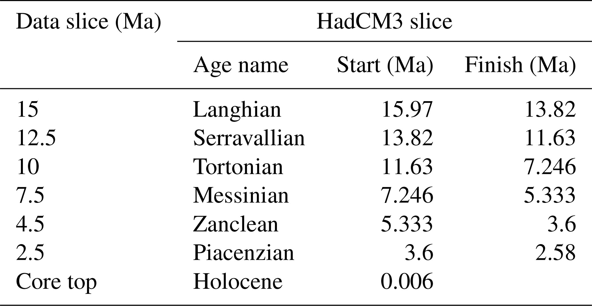
For convenience, uncertainty in model climate forcing is assumed to be represented by atmospheric CO₂ – this should be understood as an “equivalent” CO₂ forcing that encompasses changes in all atmospheric greenhouse gases (especially methane). Ocean circulation in the model is a function of surface ocean boundary conditions (especially wind stress) and climate (including atmospheric CO₂ forcing), ocean bathymetry, and the existence and nature of seaways and gateways – all of which we adjust at each time slice (along with the solar constant). We further introduce a variable (parameter uncertainty) to the model that alters the salinity transfer between the North Pacific and North Atlantic – a classic “flux adjustment”. This represents the effect of atmospheric moisture transport and the relative precipitation that east- vs. west-draining watersheds receive on the North American continental land mass, none of which can be resolved well in the simple 2D energy–moisture balance model-based approach employed here (Edwards and Marsh, 2005; Marsh et al., 2011). This “flux correction” results in an Atlantic Meridional Overturning Circulation (AMOC) being induced (and/or strengthened) in cGENIE and, hence, represents a parameter “knob” in trying to find a fit to ocean proxy data. (Indeed, it is required in the standard present-day configuration (Ridgwell et al., 2007; Marsh et al., 2011) in order to rectify the aforementioned simplification in modelled atmospheric moisture transport and dynamics.)

2.1 Data sets

We selected published surface ocean temperature data based on either alkenones or TEX₈₆ for all seven slices (with the exception of two data points at 15 Ma), noting that our selected proxies, like any proxy, are still subject to uncertainties and limitations, such as seasonality effects, surface/subsurface water representation, or non-thermal influences (discussed in Richey and Tierney, 2016, for ${\mathrm{U}}_{\mathrm{37}}^{\mathrm{K}}$ and TEX₈₆). Figure 1 shows surface temperature data locations, and Supplement A contains the data set. For slices 2.5 to 15 Ma, published benthic δ¹³C and δ¹⁸O data were selected only for the Cibicidoides and Planulina foraminifera species. These species were selected so that temperature could be calculated from shell δ¹⁸O using the linear model from Marchitto et al. (2014) in order to reduce uncertainty driven by species-specific effects on shell isotopic signatures. We ensured that at least 15 data points were available for each time slice and that coverage included the Atlantic and Pacific basins (Fig. 1 shows the benthic data locations, Fig. 2 shows the δ¹³C data plotted by palaeolatitude, and Supplement B provides the data set). Final benthic temperatures calculated from δ¹⁸O consider the effect of benthic water salinity on δ¹⁸O_sw which, in turn, is influenced by ocean circulation (the calculated temperatures in Table S2 in the Supplement are uncorrected for salinity), and we use the modelled benthic salinity field to create the correction for the local water δ¹⁸O_sw. The method used in this calculation is described in detail in Appendix A. Palaeo-locations for each data point were found using the reconstructions from http://www.paleolocation.org/ (last access: 11 October 2021) (Urban and Hardisty 2013) that provide Zanclean (4.466 Ma), Tortonian (9.427 Ma), and Burdigalian (18.2 Ma) palaeo-locations using PLATES reconstructions (University of Texas, 2015). Thereafter, the palaeo-locations for each data point at our time slices (Table 1) were interpolated using these three points and the present-day location in a cubic model regression.

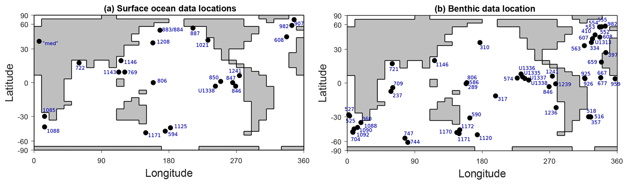
Figure 1 Present-day location of surface ocean temperature data points (a) and benthic δ¹⁸O and δ¹³C data points (b) collated for this study (the Holocene δ¹³C data set from Peterson et al., 2014, is not plotted).

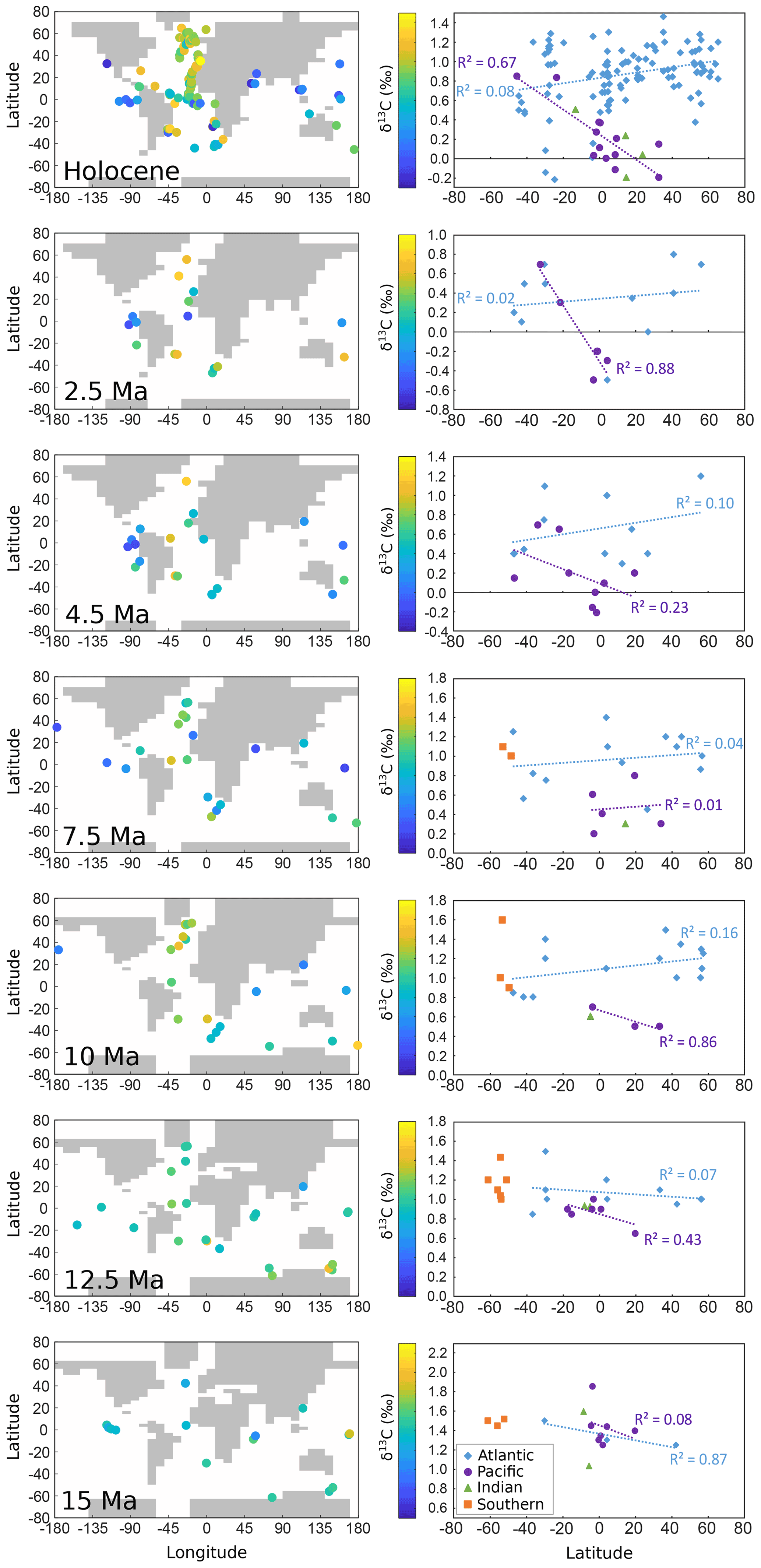
Figure 2 Benthic δ¹³C data and palaeo-locations overlaid on palaeo-coastlines (left column). Benthic δ¹³C data plotted by latitude for each time slice, showing the linear regression and R² for the Atlantic and Pacific basins (right column). The colour scale for the map is also the y axis scale for the per-latitude data, and all axes have a range of 1.8 ‰.

To account for age model uncertainties in the isotope data, a window of ±1 Myr was inspected for each δ¹⁸O and δ¹³C data point to ensure that the data value was not unrepresentative of the general value at that site around the target age (rather than taking a mean value over a certain window of time). This approach was applied to try to ameliorate the effect of uncertainties in age models, particularly for periods in which isotope values change significantly over the 2 Myr interval. In data sets with high resolution (i.e. showing possible orbital-type climate cycling) and generally better age models, an intermediate value between the high and low nearest to the target age was selected (thereby targeting mid-climate states). All of the data points and their palaeo-locations as well as the ± million-year time series plotted for each data location are available in Supplement C, Fig. S1.

We created data sets for the late-Holocene time slice slightly differently. For this, we took the Holocene benthic δ¹³C from Peterson et al. (2014). For ocean temperature, we used data from the World Ocean Atlas (WOA) 2009 (Levitus et al., 2010), assuming that deep-ocean temperature has changed little between the late Holocene and the present. Data points for the deep ocean (at 4000 m) were extracted from WOA 2009 to create the benthic temperature data set for model–data fit statistics (only data locations where the cGENIE model's seafloor depth closely matched the WOA 2009 seafloor depth were used).

2.2 The cGENIE.muffin Earth system model

We run the open-source intermediate-complexity Earth system model cGENIE (“muffin” release) (see the “Code availability” section for details). As implemented in our study, this comprises (1) a 3D ocean circulation model configured on a 36×36 equal area grid with 16 non-equally spaced vertical levels in the ocean, (2) a 2D energy–moisture balance atmospheric model (EMBM) component, and (3) a 2D dynamic–thermodynamic sea-ice model component. These three individual components and their coupling are described in Marsh et al. (2011, and references therein). The basic physics parameter calibration of the climate model component is as per Cao et al. (2009) unless described otherwise. For the modern Atlantic Basin configuration (and, as per the findings of this paper, also over the past 15 Ma), the lack of both atmospheric dynamics and explicit topography on land in our configuration model requires that a freshwater flux adjustment is applied. This is implemented in the modern configuration of the model, principally by transferring salinity to the North Atlantic region from the North Pacific as described in Edwards and Marsh (2005), although we deviate from this flux pattern as described in the following.

Our implementation of the cGENIE model includes a relatively complete description of the cycling of carbon and oxygen in the ocean as well as exchange with the atmosphere, as described in Ridgwell et al. (2007) and Cao et al. (2009). In addition, the carbon isotopic (δ¹³C) composition of all of the carbon pools as well as associated fractionations between them are explicitly account for, as described in Ridgwell et al. (2007) and with additional description and evaluation in Kirtland Turner and Ridgwell (2016). Given the paucity of constraints on the evolving patterns of aeolian fluxes to the ocean surface, we omit a marine iron cycle and include only a single nutrient (phosphate) as potentially limiting to biological productivity in the ocean in our configuration. We also employ an idealised organic matter export scheme and, hence, biological carbon pump (Cao et al., 2009) and do not attempt to simulate ecosystem composition and dynamics (as per, for example, Wilson et al., 2018).

In the original modern configurations of the cGENIE model, ocean bathymetry and land–sea mask grids as well as files supporting the calculation of ocean circulation files (defining “islands” and circulation paths around islands) are derived from filtered global topographic observations (ETOPO5) (Edwards and Marsh, 2005). Furthermore, because the atmospheric EMBM component lacks clouds and dynamics (e.g. winds), additional spatial fields must be provided as fixed (annual average) boundary conditions. Firstly, a zonally averaged planetary albedo profile is applied (originally as a simple cosine function of latitude as per Edwards and Marsh, 2005). Secondly, fields for (a) vectors of wind stress on the ocean surface, (b) vectors of surface wind velocity in the atmosphere, and (c) short-term wind speed are derived from modern observations and applied to (a) driving surface ocean circulation, (b) transporting heat and moisture in the atmosphere and for calculating heat and moisture exchange between the ocean surface and atmosphere, and (c) in calculating air–sea gas exchange respectively.

For this study, we create a series of new continental and surface boundary condition configurations of the cGENIE model for the seven time slices spanning the late Holocene through to mid-Miocene. As per previous (deeper time) palaeo-applications of the cGENIE.muffin model (e.g. Ridgwell and Schmidt, 2010), rather than observations, we derive the required boundary conditions from a representative fully coupled GCM (general circulation model) experiment. To create the Miocene slices' boundary conditions, we re-grid the GCM HadCM3LM2.1aE (hereafter referred to as HadCM3L) model configuration to the cGENIE grid using the method described in Appendix B, including bathymetry, wind stress and velocity, and planetary albedo. Due to the re-gridding process, this results in an open Central American Seaway (CAS) from 15 Ma up to and including the present (late Holocene). To test for the role of closing the CAS, we create a parallel series of an additional five time slices spanning 10 Ma to present, in which we force a fully closed CAS in the cGENIE model grid. (Although the CAS is not open today, we include an open CAS for the late-Holocene time slice for completeness and to test for the ability of benthic δ¹³C observations to distinguish between the two alternatives.) The resultant cGENIE bathymetry for each time slice is shown in Fig. 3 for all 12 (7 open-CAS and 5 closed-CAS) continental configurations, with a close-up section around the CAS and a cross section of the shallowest CAS depths for each open CAS configuration. We compare our PLATES-derived palaeo-locations to those derived from the HadCM3L in Fig. B1.

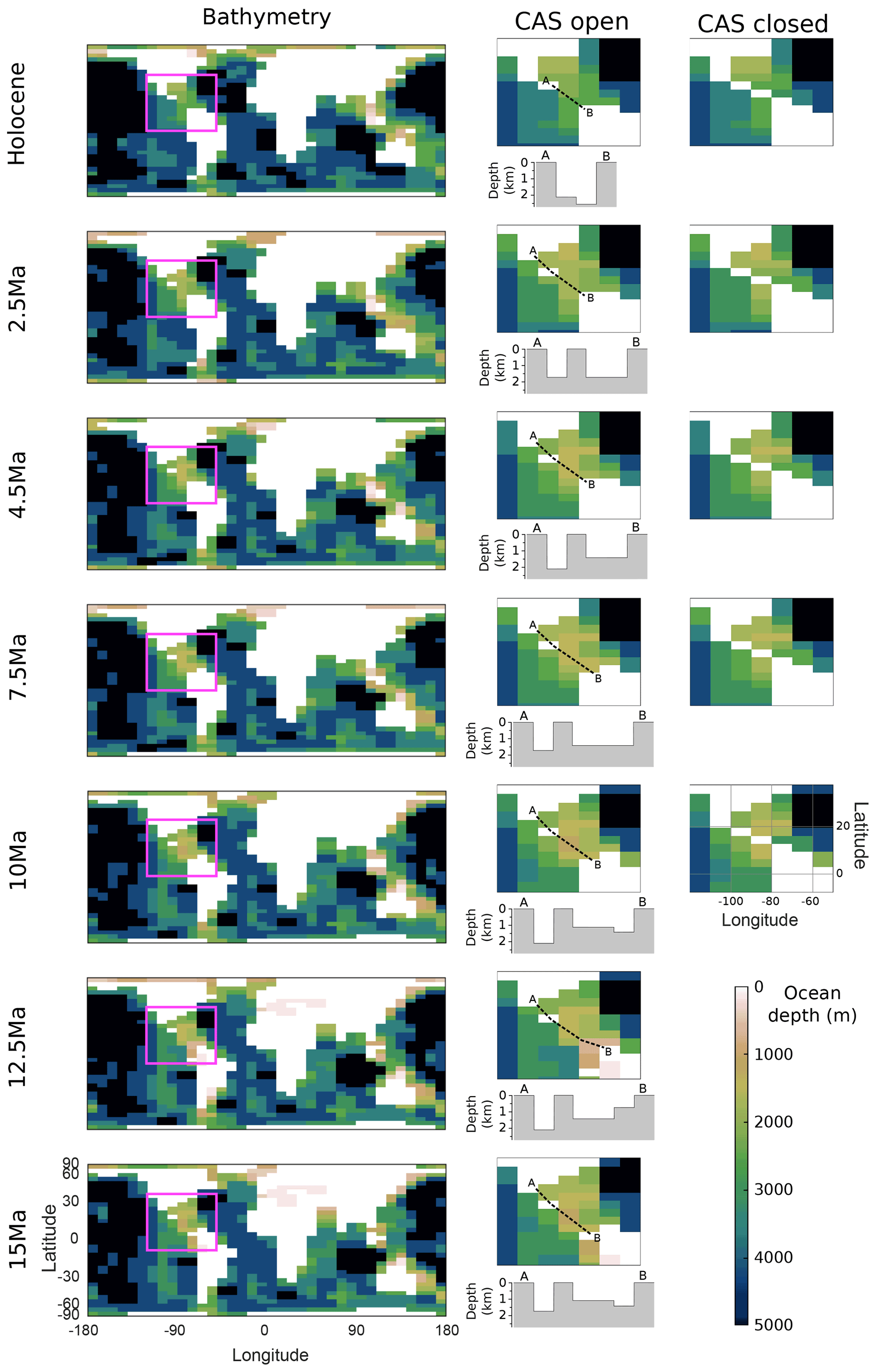
Figure 3 Model bathymetry and coastlines for each time slice, and a close-up of the region covering the Central American Seaway (CAS), including a transect showing the most depth-restricted pathway for the open-CAS configurations and the ocean depths for both open- and closed-CAS configurations.

The impact of changing grid resolution and swapping the HadCM3L physics for that of the cGENIE model on the ocean circulation is included in Fig. B2 in the form of a comparison of modern (late-Holocene) simulations. HadCM3L generally shows much stronger currents, such as the Antarctic Circumpolar Current (ACC), than cGENIE, with the finer-resolution HadCM3L enabling features like the western boundary current in the Atlantic to be reasonably resolved, whereas it appears weak and diffuse at much lower resolution in cGENIE. In addition to the lower-resolution model grid employed in this study, the frictional geostrophic approximation physics employed in cGENIE (Edwards et al., 1998) also tends to dampen the wind-driven circulation. However, the fidelity of the large-scale patterns of ocean circulation in cGENIE is sufficient to support the simulation of anthropogenic carbon uptake and deep-ocean radiocarbon on par with other 3D ocean-circulation-based Earth system models (Cao et al., 2009) as well as generally plausible distributions of dissolved nutrients and oxygen (e.g. Crichton et al., 2021).

2.3 Model experimental design

In a “perfect” palaeo-model (which does not exist) and under the correct greenhouse gas boundary conditions (which are poorly constrained), climate and ocean circulation would be a correct and emergent property of the model and would provide an exact (within proxy measurements and calibration error) match to the data. Rather, the premise of our experimental design and study is that we can find a specific combination of climate state and pattern of global ocean circulation that reasonably accounts for the observed distribution of ocean temperature proxies and benthic δ¹³C. In cGENIE, we consider CO₂ as a primary uncertainty in the model – not only in terms of uncertainty in the real past value but also with respect to the radiative forcing required in cGENIE to generate appropriate ocean temperatures. Additionally, because there is no prior expectation that the emergent state of ocean circulation is at all correct for a “correct” surface climate in cGENIE, we consider the salinity flux adjustment (hereafter “FwF”) as an additional “unknown” and also as a means to an end in adjusting basin-scale (to global-scale) patterns and the strength of circulation (specifically Atlantic overturning circulation). By varying both controlling factors (parameters), we seek to find the circulation pattern and climate (temperature) state that best reproduces the data. It should be noted that we ignore the strength of the biological pump as an additional and independent control on benthic δ¹³C for this study, and in our particular model configuration, remineralisation rates of organic matter in the ocean interior are not dependent on local temperature. Similarly, we assume the modern ocean nutrient (phosphate) inventory throughout all time slices.

For each of the 12 (7 open-CAS and 5 closed-CAS) time slices and model configurations, we carry out a 2D parameter space (CO₂ vs. FwF) sweep via an ensemble of model experiments. In each ensemble, we test (radiative forcing equivalent) atmospheric CO₂ values of 280, 400, 560, 800, 1120, and 1600 ppm, and vary the salinity flux correction applied to the North Atlantic (FwF) between 0.0 and 0.7 Sv, in increments of 0.1 Sv, for a total of 48 members in each ensemble. The CO₂ values are chosen as either simple multiples of 280 ppm (pre-industrial/late Holocene), or commonly assumed GCM values (e.g. the 400 ppm in Farnsworth et al., 2019) and multiples thereof. We chose the range of FwF values to encompass the equivalent tuned modern cGENIE model value of 0.32 Sv (Edwards and Marsh, 2005). Furthermore, because the land–sea mask progressively changes across the seven time slices, we create a common mask for the purpose of salt transfer: first, we identify all of the grid points that are ocean (“wet” points) across all configurations and that lie northwards of the northernmost extent of the CAS, and we add salinity to these; second, we identify all of the grid points outside of the North Atlantic that are ocean in all configurations, and we remove salinity from these; finally, the total FwF value is divided evenly across all (equal area) grid points in the North Atlantic (positive salinity input) and “elsewhere” (negative salinity input) such that global ocean salinity is always conserved. The mask is shown in Fig. B3.

For each ensemble member and each time slice (a total of $\mathrm{48}\times \mathrm{12}=\mathrm{576}$ model simulations), we spin-up the cGENIE model for 10 000 years. In the absence of appreciable inter-annual variability and unlike in fully coupled GCM experiments, multi-decadal averaging is not necessary in the cGENIE model; thus, we take the last annual average (year 10 000) of the simulation in order to carry out the model–data comparison.

The one caveat and complication regarding how we conduct the model–data comparison is that, in running the parameter ensembles, we identified self-sustained oscillations in global ocean circulation in a subset of the simulations that affected both mean benthic temperature (up to several ^∘C) and δ¹³C (several tenths of a ‰). These oscillations were of varying period and magnitude and occurred only in simulations with sea-ice cover present (and, hence, in the lower range of eq.CO₂ forcing), and generally for the low to middle range of FwF values (see Appendix C and Fig. C1 for more details). Whilst this raises extremely interesting questions about past ocean circulation dynamics, it is not the focus of this study (although it will be followed up in a subsequent study). Here, we need to identify a “representative” ocean state of the model in order to carry out the model–data comparison consistently. Therefore, to create a representative state for each CO₂–FwF combination, we parsed the ensemble cGENIE model output, identifying ensemble members characterised by self-sustained oscillations. For these ensemble members, we identified the period of the oscillation and averaged the model output over one full period, starting the average from the end of the 10 000-year spin-up and working back (towards the start of the model experiment). Both unmodified run-end and reconstructed mean annual averages were then treated exactly the same in terms of carrying out model–data comparison.

2.4 Model–data comparison

The collated data sets were used as an observational constraint to determine which combination of CO₂ and North Atlantic salinity flux correction (FwF) produces the best fit ocean state to the data. This is performed quantitatively by statistically comparing local model output with the data points for all three data sets and combining these to produce a final “best fit” model setting for each time slice. The statistical methods applied are as follows: (1) the difference between the mean of the data set and the mean of the model output at the data locations, producing an offset value or mean bias, and (2) an overall measure of goodness of fit of the model to the data set, known as the “M-score” (Watterson, 1996). Where several data points are located within one model grid square, the mean of the data values is used for comparison with the model value. For the benthic data, each data point is assumed to be on the ocean floor, so the model's bathymetry determines the data depth, and the data value is compared with the model value in the deepest water in that location.

3 Results

3.1 Global mean and spatial data constraints

We start by assessing the model ensemble members against global mean observational constraints. In Fig. 4, we show the global mean benthic temperature data estimate from Cramer et al. (2011) plotted on top of the modelled global mean benthic (seafloor arithmetic mean) ocean temperature for our ensemble. Both CO₂ and FwF have a strong effect on benthic temperature. Bathymetry, albedo, and wind fields (which differ in our time slices; see Appendix B) also have a direct effect on benthic ocean temperature, with 15 Ma having a tendency toward a warmer deep ocean compared with other time slices, even for the same CO₂ and FwF in the open-CAS cases. A range of combinations of CO₂ and FwF would satisfy the global mean benthic temperature constraint (shown as the dashed white line in Fig. 4, with the range shown using thin white lines). The FwF affects North Atlantic surface salinity and, therefore, has an impact on thermohaline circulation; higher FwF values create more saline surface North Atlantic waters of lower buoyancy, transporting more of the surface heat to the deep ocean. This results in combinations of higher CO₂–low FwF or lower CO₂–high FwF being equally possible to satisfy the benthic global mean temperature constraint, although with a general trend from 15 Ma towards the Holocene of decreasing CO₂ and FwF (as the dashed line moves towards the top left in Fig. 4) for both the open-CAS and closed-CAS cases. For almost all slices, an elbow-type shape is present in the modelled benthic temperatures. As CO₂ decreases for a given FwF, the global mean benthic temperature is either stable or even increases at a certain point (Fig. 4). At CO₂ levels lower than this “elbow”, the cooler surface ocean favours the sinking of waters at high latitudes, supporting the thermohaline circulation. At 12.5 Ma, the elbow turning-point CO₂ value is around 800 ppm, and this gradually decreases to about 400 ppm in the Holocene (for mid-range FwF). At CO₂ higher than this elbow, there is only a weak (or shallow) AMOC. In the closed-CAS cases, this elbow is less evident than for the open-CAS cases, which may suggest that an open CAS results in a climate more (or differently) sensitive to CO₂ changes than a closed CAS, via AMOC.

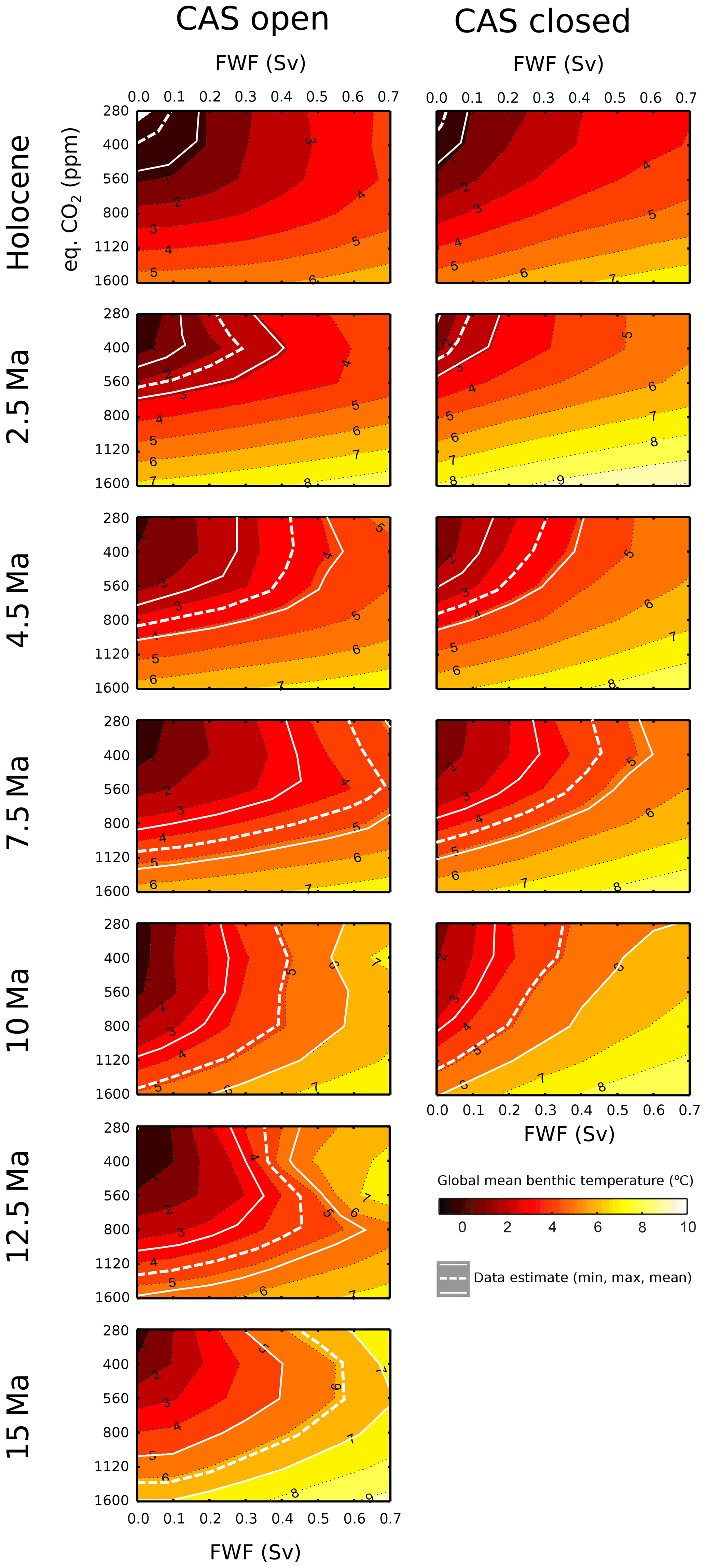
Figure 4 Modelled benthic temperature with the global mean temperature estimate (and minimum and maximum range) (Cramer et al., 2011) overlaid (dashed line and solid white lines respectively). The global mean temperature shown for the Holocene time slice denotes 0.1 Ma, representing a mean value for the Pleistocene glacial–interglacial climate.

The results of the M-score spatial statistical comparison (the closer the value is to 1, the better the model can simulate the data) for the three individual data sets and all model ensemble members are shown in Fig. 5, where the FwF from 0.0 to 0.7 is plotted sequentially for each eq.CO₂ forcing.

Figure 5 The M-score for the fit of the model to data for surface temperature, benthic temperature, and benthic δ¹³C. The model settings are plotted on the y axis (totalling 48 simulations per chart).

The surface temperature constraint is rather insensitive to FwF, with eq.CO₂ being the main controller on the fit to data. Whether the CAS is open or closed also has very little effect on the ability of the model to reproduce the data. The highest M-scores indicate that a general fall in eq.CO₂ forcing results in the best fit to the surface temperature data, with generally higher M-scores achieved in the more recent time slices. The 12.5 and 15 Ma time slices have low scores (less than 0.4) compared with other time slices for surface ocean temperature, indicating that, even at 1600 ppm, the model cannot reproduce the data-indicated surface ocean temperatures very well.

For the benthic temperature data set, as for the global mean ocean temperature (Fig. 4), both eq.CO₂ and FwF control deep-ocean heat distribution, with the highest M-scores again generally showing decreasing CO₂ and decreasing FwF towards the present. The open-CAS case results in higher M-scores (i.e. better fit to data) than the closed-CAS case, even for the Holocene. As we know that the CAS is closed in the Holocene, these higher M-scores may be the result of a model bias.

The δ¹³C M-scores for the Holocene show higher values for a closed CAS than for an open CAS, indicating that δ¹³C may be a better indicator than benthic temperature for whether CAS is open or closed in our cGENIE model configurations. For the 10 Ma slice, a closed CAS better fits benthic δ¹³C data for a higher CO₂ value, and if gradually decreasing CO₂ is assumed (from the surface temperature data) toward the present, a closed CAS generally results in higher M-scores for all other time slices as well. A shift occurring in the patterns of benthic δ¹³C can also be seen in the raw data. The latitudinal trend for δ¹³C data (dotted lines) in Fig. 2 shows that the Atlantic appears to switch trend between 12.5 and 10 Ma. Prior to 12.5 Ma, the North Atlantic data indicate a generally more negative δ¹³C than in the South Atlantic – a situation that reverses from 10 Ma onwards when more positive δ¹³C values tend to occur in the North Atlantic (although R² is low). In the Pacific Ocean, the δ¹³C gradient from south to north tends to intensify towards the present, with the largest gradient seen at 2.5 Ma. Overall, the range of δ¹³C values increases from 15 Ma towards the present. (Note that the colour bar values change, but the range – the difference between the minimum and maximum value – is 1.8 ‰ for all time slices in Fig. 2.)

3.2 Combining the constraints

All proxy data constraints combined are shown in Fig. 6, the surface and the deep-ocean temperature constraints (showing both M-scores and regions where the bias in deep-ocean temperature is less than 2 ^∘C), and the global mean benthic temperature estimates are mapped onto the statistical fit surface (M-score) of model vs. observed δ¹³C. We mark the best fit selection with a star and include a range of estimates delineated by whiskers on the best fit CO₂ and FwF values. Note that the best fit is only identified from those specific values for which we ran the model ensemble members (i.e. we do not interpolate between settings).

Figure 6 All proxy data constraints combined. The M-score for the modelled benthic δ¹³C fit to the data set is shown using filled contours (grey). The modelled benthic global mean temperature nearest to that identified in Cramer et al. (2011) is shown using a dashed white line, with the maximum and minimum estimates shown as solid thin white lines. The benthic temperature constraint is shown using blue; the blue filled region is where modelled benthic temperature has a bias of less than <2 ^∘C with respect to the δ¹⁸O-derived temperature data (or the WOA 2009 for the Holocene), and the blue contour indicates the M-score, with the value given in blue. The M-score contour for the modelled surface ocean temperature fit to data is shown using red shading, with the value marked on the edge of the contour. The overall best fit settings are shown using a white star, with the upper and lower range estimates shown using whiskers.

It is clear from this that the primary constraint on atmospheric eq.CO₂ in the model in this study is the proxy-reconstructed surface ocean temperature. This is much less sensitive to the FwF value than the other benthic ocean constraints. This is because surface ocean circulation patterns are largely dictated by the wind stress forcing, which we do not vary within any single time slice. Given a surface ocean circulation pattern that is relatively immune to changes in the applied FwF, the ensemble member eq.CO₂ value and the surface climate state control the mean and pole-to-Equator gradient of sea surface temperature (SST) and, hence, the model–data surface temperature fit. Thus, for all of the following model–data fit analyses, we start by considering SSTs and the choice of eq.CO₂ for each respective time slice and then bring in additional constraints and consideration of the value of FwF.

A priority for selecting good combinations of eq.CO₂ and FwF values is to ensure that the global ocean heat distribution shows reasonable agreement with our proxy temperature data. The benthic global mean temperature estimate of Cramer et al. (2011) is then used as an ancillary guide for our benthic temperature set derived from δ¹⁸O and the salinity correction; in most cases, these show quite good agreement with one another (with 15 Ma and both of the Holocene cases showing the lowest agreement; note that the Cramer et al. (2011) estimate applied for the Holocene actually represents a mid-climate state rather than the interglacial, which explains the difference there). It should be noted that the global ice-volume-linked global δ¹⁸O_sw value that we use in our temperature calculation is derived from the Mg$/$Ca temperature data set from Cramer et al. (2011) (Table S2 in the Supplement), so these are not fully independent data sets. The M-score for the δ¹³C is used to determine the direction of any adjustment needed when SST and benthic temperature constraints have low agreement for the best eq.CO₂–FwF combination, especially for particularly high δ¹³C M-scores (e.g. for the 10 Ma open-CAS case, where benthic temperature suggests an FwF value of 0.1 Sv and an eq.CO₂ value of 1120 ppm, but the δ¹³C M-score strongly increases in the direction of lower CO₂ and higher FwF values). More details on the selected combinations are available in Appendix D. All of the selected settings for eq.CO₂ and FwF and their ranges are summarised in Fig. 7 (and marked in Fig. 5), along with some recent data estimates of atmospheric CO₂. Also plotted in Fig. 7 are global mean ocean surface and benthic temperatures as well as sea-ice extent and thickness for each time slice, showing the modelled evolution from 15 Ma to the Holocene.

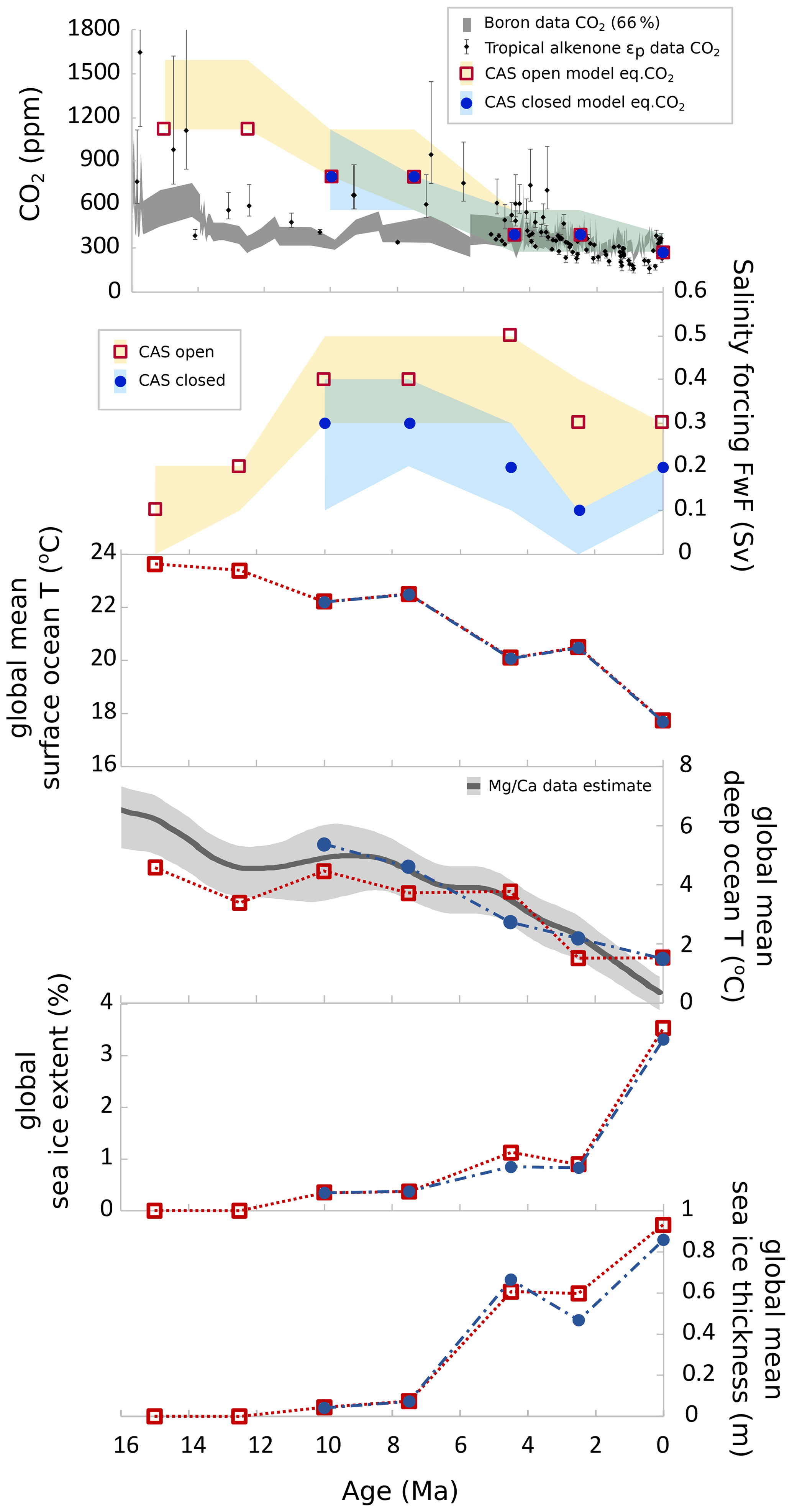
Figure 7 The eq.CO₂ and FwF settings (and estimated ranges) that agree with temperature and benthic δ¹³C data constraints according to this study. Plotted with eq.CO₂ are estimates for atmospheric CO₂ levels from two recent studies on tropical alkenones (Stoll et al., 2019) and boron (Sosdian et al., 2018). Also shown are modelled global mean surface ocean temperature, global mean benthic ocean temperature (and the Mg$/$Ca thermometer estimate from Cramer et al., 2011), modelled global sea-ice extent, and modelled global mean sea-ice thickness for the best fit settings.

Modelled surface ocean temperature drops with decreasing eq.CO₂; deep-ocean (benthic) temperatures also fall, but they show some dependence on FwF at the same time (Fig. 7). In the highest FwF case (4.5 Ma, open CAS), despite a halving of eq.CO₂ compared with 7.5 Ma, deep-ocean temperatures are only slightly lower than 7.5 Ma. This is due to more saline North Atlantic waters and cooler polar temperatures (demonstrated by the presence of more sea ice) promoting the sinking of these surface waters to the deep, thereby delivering relatively more surface heat to the deep ocean at 4.5 than at 7.5 Ma. Conversely, in the 2.5 Ma open-CAS case, FwF is lower than at 4.5 Ma, but eq.CO₂ is the same. Here, less of the surface heat is delivered to the deep ocean, resulting in a cooler deep ocean but a warmer surface ocean and lower sea ice than at 4.5 Ma (for the best fit setting). Sea ice is present from eq.CO₂ levels of 800 ppm from 10 Ma, generally increasing with respect to both extent and thickness with decreasing eq.CO₂ (with the exception of the previous example), irrespective of whether the CAS is open or closed.

It should be noted that the imposed eq.CO₂ does not change due to changes in ocean carbon distribution or carbon exchange with the atmosphere; we apply a flux correction such that atmospheric CO₂ is always restored to the eq.CO₂ value that we initially impose; therefore, we do not attempt to attribute the source of CO₂ decline since 15 Ma to any particular mechanism.

3.3 Atmospheric and global mean benthic carbon-13 ratios

Using the CO₂ FwF settings identified from the combined constraints, we can derive model-predicted estimates of the trends in atmospheric δ¹³CO₂ and of global mean benthic δ¹³C over the past 15 Myr. In the ensembles, the model atmosphere is forced with a δ¹³CO₂ value of −6.5 ‰ for all simulations; thus, by determining the mean bias between the modelled benthic δ¹³C points and the data benthic δ¹³C points, we can derive the δ¹³CO₂ value that would produce the lowest overall model–data error (thereby essentially inverse modelling the δ¹³CO₂ value). This is shown in Fig. 8. This diagnosed history of atmospheric δ¹³CO₂ can be used as a means of identifying changes in the global carbon cycle (e.g. Hilting et al., 2008) or as initial condition values for future model-based (and model–data-based) studies.

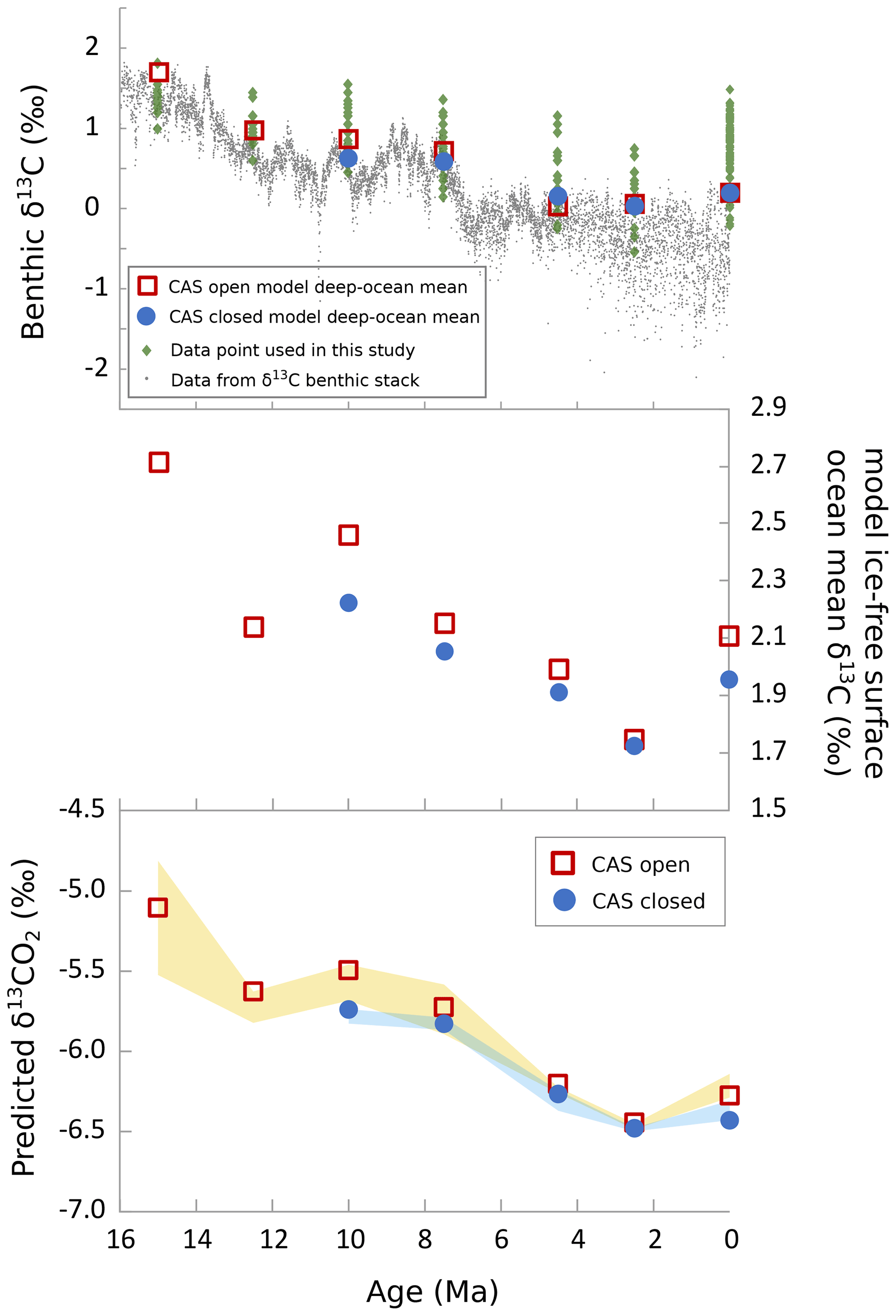
Figure 8 Inferred global benthic mean δ¹³C, global mean surface ocean δ¹³C, and atmospheric δ¹³CO₂ calculated using the mean bias of the best fit model to the data-indicated benthic ocean δ¹³C in each time slice. The data points from the δ¹³C benthic stack are from Westerhold et al. (2020). The shaded regions for predicted δ¹³CO₂ show the range of δ¹³CO₂ using the best ranges identified in Fig. 6.

Similarly, using this model–data benthic δ¹³C bias we can derive the global surface and benthic mean δ¹³C trend using the local bias of our model to the benthic δ¹³C data. This global mean deep-ocean δ¹³C is shown in Fig. 8 and is plotted along with the benthic δ¹³C stack from Westerhold et al. (2020). The data points from our benthic δ¹³C data set are also shown in Fig. 8 and tend to be higher (especially in younger time slices) than the benthic stack data; unlike the benthic stack data, our benthic data set is not limited to low latitudes and mid-latitudes (see Fig. 2). The North Atlantic data points generally have more positive δ¹³C values than other regions, and a large proportion of our data points are from this region. We use local model–data benthic δ¹³C differences to constrain the global benthic δ¹³C mean, but we still find this mean to be on the higher (heavier) end of the benthic δ¹³C stack from Westerhold et al. (2020). The modelled surface and deep-ocean mean δ¹³C falls by around 0.8 ‰ between 15 Ma and the Holocene, whereas atmospheric δ¹³CO₂ falls by up to 1.5 ‰ at the same time.

3.4 Best fit model–data maps

In general, in the older time slices, cGENIE underestimates temperatures in the North Atlantic (Fig. 9), and this results in a higher M-score for the highest CO₂ settings for the 15, 12.5, and 10 Ma slices (see Fig. 5). In these older time slices, the model high-latitude temperatures tend to be too low compared with data: this is an established characteristic of warm climates, where climate models tend to struggle to reproduce the flatter latitudinal temperature gradients seen in data (Goldner et al., 2014). Whether the CAS is open or closed makes little difference to the model–data fit, as our data points are not in regions that are very strongly affected by any resulting change in surface heat distribution. However, the temperature difference map shows that a closed CAS results in a colder modelled South Atlantic surface ocean than an open CAS as well as a slightly warmer Pacific surface ocean (note that although the FwF values are not the same between the cases, it is the CAS configuration that dominates the surface ocean temperature differences). These temperature differences of 1 or 2 ^∘C at high latitudes would have implications for sea-ice and ice-shelf growth in the cooler time slices.

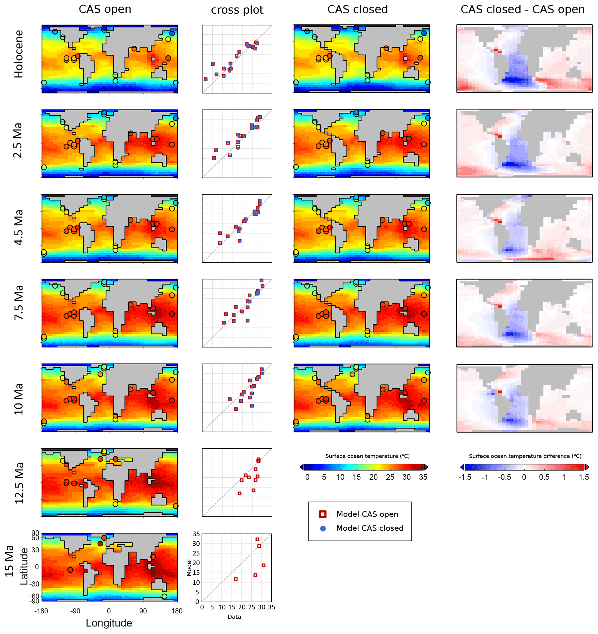
Figure 9 Modelled and data-indicated surface ocean temperatures for the best fit model settings, with data overlaid as shaded circles (temperature maps), and cross plots of data points (x axis) and model points (y axis) for both CAS cases. The surface temperature difference is shown on the right. The model–data fit statistic (M-score) is shown in Fig. 5.

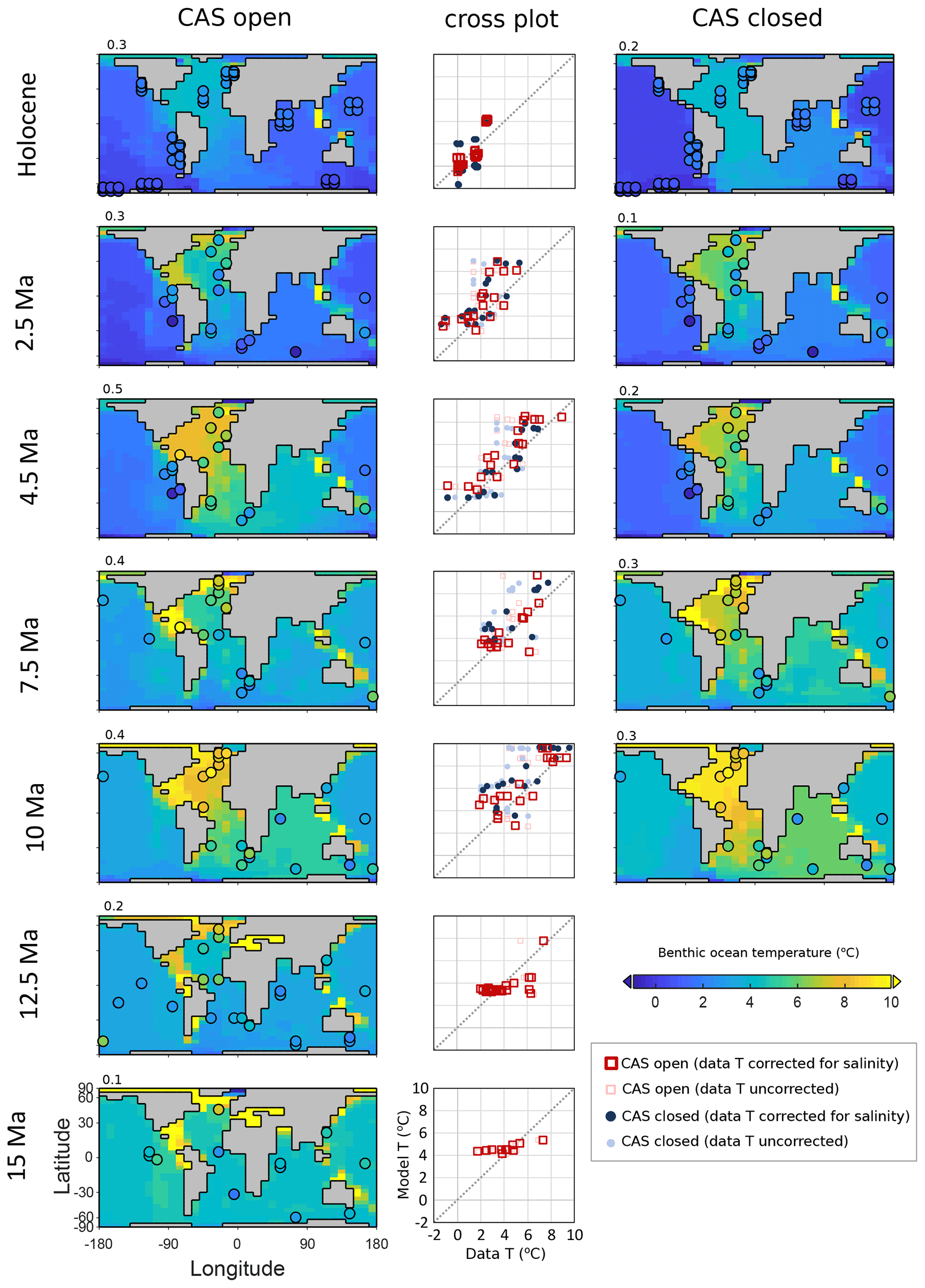
Figure 10 Benthic temperature for the best fit model settings, with data overlaid as shaded circles, and cross plots of data points (x axis) and model points (y axis), with temperature calculated with no salinity correction (semi-transparent) and with salinity correction (opaque). Noted above each map is the FwF setting (in Sv). The model–data fit statistic (M-score) is shown in Fig. 5.

Taking account of the deep-ocean salinity in the temperature calculation with δ¹⁸O data makes a significant difference to deep-ocean temperature patterns (Fig. 10). When flux corrections are higher (mainly from 10 Ma), the saltier North Atlantic waters are less buoyant and sink more readily. This higher salinity results in higher calculated temperatures (as δ¹⁸O_sw is corrected for local salinity), with data points in shallower waters most strongly affected (see Appendix A). Accounting for water salinity increases some data points' temperature by more than 3 ^∘C (Fig. 10) in the North Atlantic. The inverse is true for data locations in the deep Pacific, where some temperatures are corrected lower. In both cases, this affects the model–data fit, likely resulting in higher CO₂ and/or higher FwF combinations than would otherwise be the case if we had conducted the model–data comparison using only uncorrected δ¹⁸O-derived temperatures. The open-CAS case for the Holocene shows a higher M-score than the closed-CAS case for the model fit to benthic temperature (which we know should not be the case, as the CAS is actually closed in the Holocene) (Fig. 5). The Indian Ocean appears to be a location where modelled benthic temperature is too high compared with our δ¹⁸O-derived data, whereas the Pacific is generally too low (and the open-CAS case shows a better fit to data). The 2.5 Ma modelled benthic temperature is slightly too high, and this is probably due to the 400 ppm forcing, where 280 ppm would also have been a good fit (see Appendix D). The two oldest time slices show modelled benthic temperature with a much smaller range than the data indicates, which may be a result of assuming all benthic data points are located on the ocean floor in the cGENIE model grid (where ocean bathymetry is smoothed out compared with the real-world case). In general, a closed CAS results in a relatively warmer deep Atlantic and cooler Pacific than an open CAS for the best fit settings.

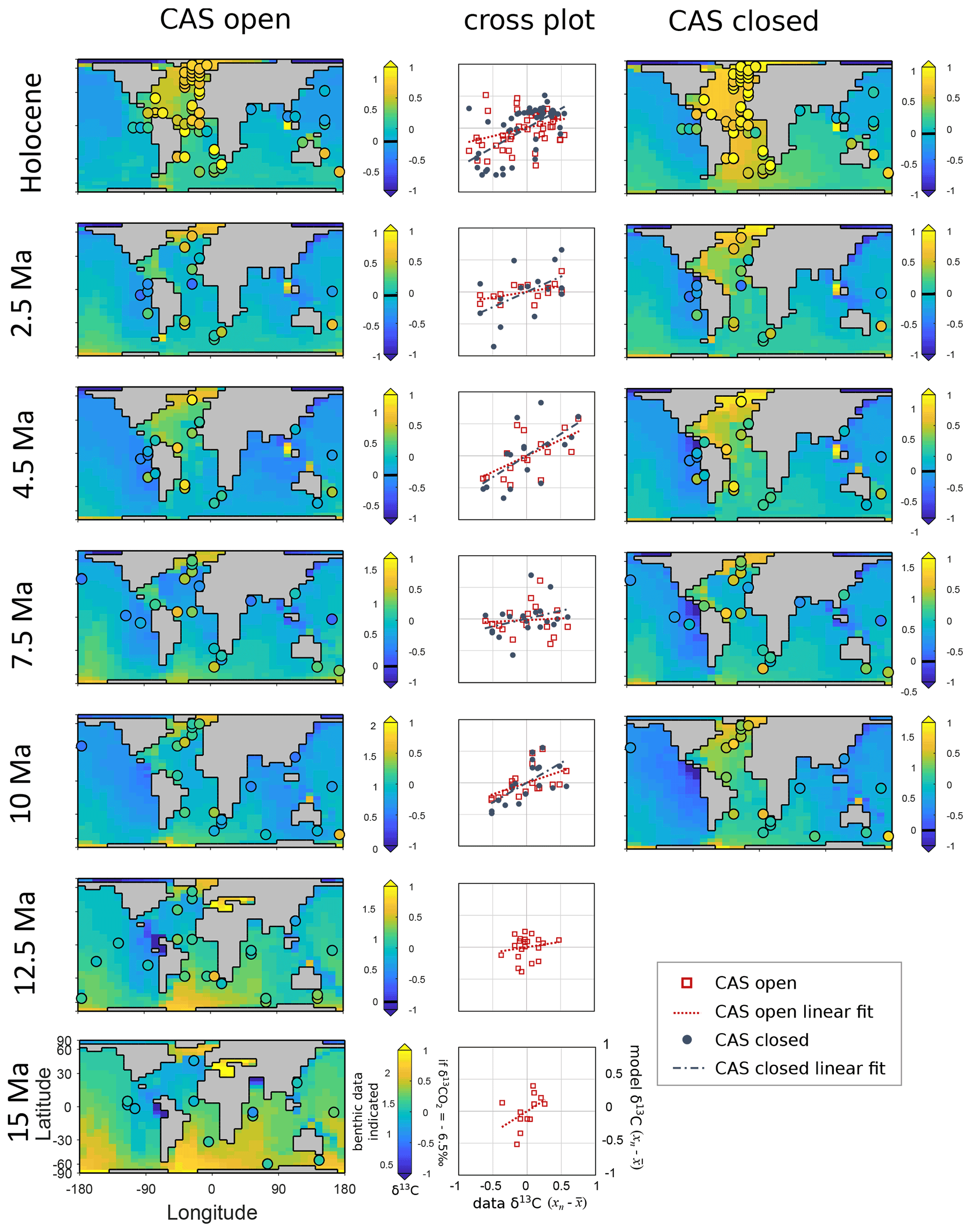
Figure 11 Modelled δ¹³C of dissolved inorganic carbon (DIC) for the best fit model settings, with data overlaid as shaded circles, and cross plots of mean-adjusted data points (x axis) and mean-adjusted model points (y axis). Note that shading is with respect to an atmospheric δ¹³CO₂ forcing of −6.5 ‰. This shading allows the comparison of the benthic ocean δ¹³C patterns between the time slices. The data-indicated δ¹³C value is shown to the left of each colour bar. The model–data fit statistic (M-score) is shown in Fig. 5.

The range of modelled δ¹³C values are in general agreement with the data-indicated range (Fig. 11). At 15 Ma, the modelled higher δ¹³C values in the high southern latitudes are not clearly shown in the data, which particularly affects the Indian Ocean. The 12.5 Ma slice shows a very low correlation for the distribution of δ¹³C. This may reflect the large climate and/or circulation changes occurring at the time (the mid-Miocene climate transition; Mackensen and Schmiedl, 2019) and the fidelity of the complied data set, especially with respect to age or, again, perhaps partly due to the smoothed model bathymetry. From 10 Ma to the Holocene, all of the closed-CAS cases show better fit to data than open-CAS cases (see also Fig. 5; the linear regression for each is shown in the cross plots (Fig. 11), and the closer this line is to diagonal, or the 1:1 line, the better the fit to data). Importantly, the model–data benthic δ¹³C correlation for 0 Ma is notably better for the closed-CAS cases than the open-CAS cases. This can also be seen in Fig. 5 where, regardless of the parameter combination, a better M-score is always obtained for a closed CAS (0 Ma) (with the exception of a single ensemble member for 0 Sv FwF and 280 ppm CO₂).

Every ensemble member, regardless of the specific atmospheric CO₂ assumption, was driven with a δ¹³CO₂ value of −6.5 ‰. The model output in Fig. 11 is colour-coded according to this value (coloured shading) so that each model time slice can be compared with any other; the coloured shading indicates deep-ocean δ¹³C relative to a universal atmospheric δ¹³CO₂ value (the data-indicated actual benthic δ¹³C value is shown to the left of each colour bar, and the scale for δ¹³CO₂ at −6.5 ‰ is shown to the right of each colour bar). As a general rule, during the warmest earlier periods, the surface ocean southern high-latitude signal dominates the deep ocean from the south, and as time progresses and the climate cools, the surface North Atlantic becomes dominant over the deep Atlantic. This is accentuated for the closed-CAS cases.

3.5 Best fit ocean cross sections

The modelled Pacific and Atlantic ocean δ¹³C cross sections are presented in Fig. 12. (Note that for benthic δ¹³C data points, we always assume that they are at the modelled seafloor, so they are not shown here.) The cross sections are for the transects shown on the inset map in Fig. 12; the mean value of model output from a swath of 30^∘ of latitude about the centre of the transect line is used to create the model ocean cross section data. Again, the coloured shading is with respect to a δ¹³CO₂ of −6.5 ‰ in order to be able to compare time slices (as in Fig. 11). In the older slices, there is a larger offset between the whole-ocean δ¹³C and atmosphere than in the younger slices (the ocean is relatively heavier in δ¹³C in older time slices). The Pacific Ocean becomes progressively more negative (lighter) in δ¹³C through time, accentuated by a closed CAS. The mid-depth mid-latitude Pacific appears sensitive to the closing or opening of CAS, with modelled δ¹³C indicating some 0.2‰–0.5‰ differences between the open- or closed-CAS cases.

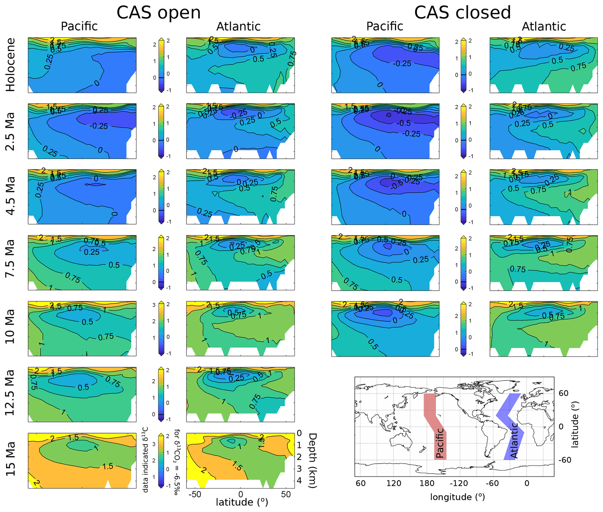
Figure 12 Pacific and Atlantic ocean cross sections of δ¹³C, where the shading and contour labelling are with respect to an atmospheric δ¹³CO₂ forcing of −6.5 ‰. This shading allows the comparison of the inner-ocean δ¹³C between the time slices, for example, 15 Ma shows values further from the atmospheric value than the Holocene. The data-indicated δ¹³C value is shown on the left of each colour bar. The inset map shows the transect locations used to make the cross sections.

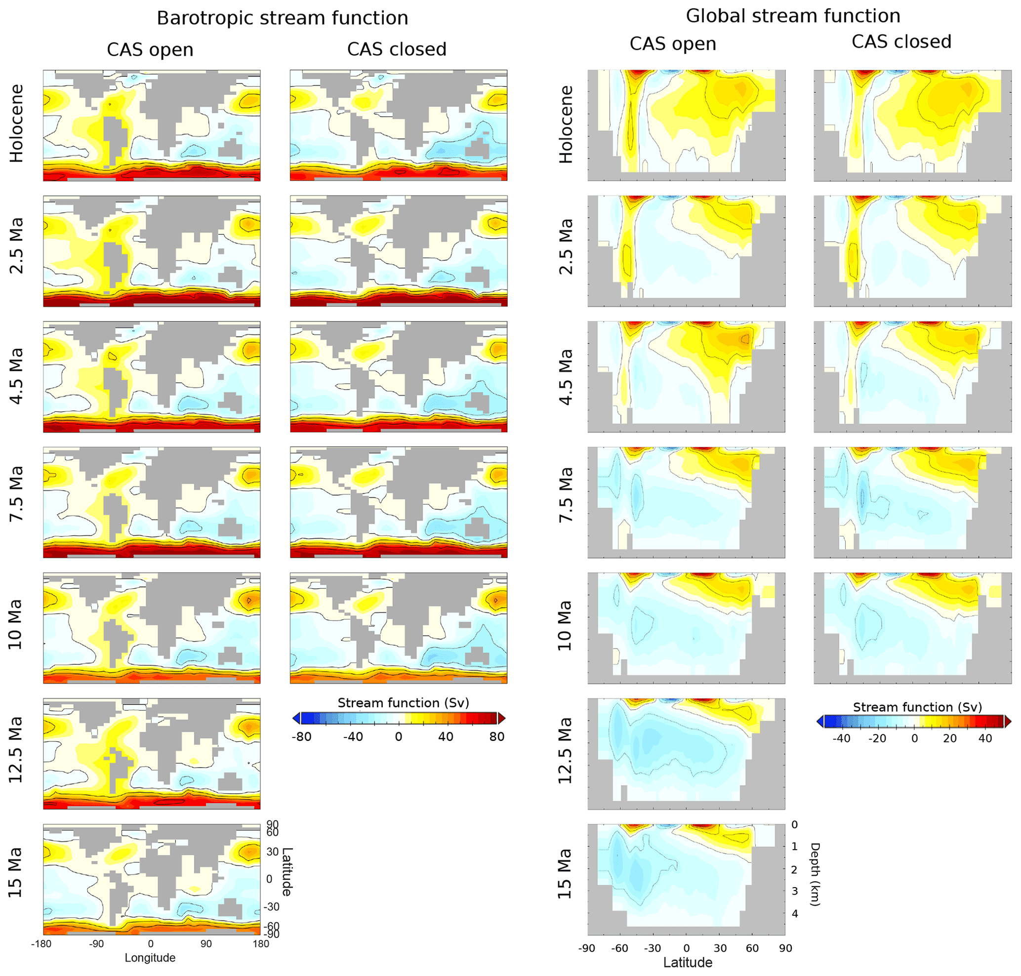
Figure 13 Modelled barotropic stream function (left) and global stream function (right) for each time slice for the best fit model settings. Contours for the barotropic stream function are at 20 Sv intervals, and contours for the global stream function are at 10 Sv intervals. Note the difference in colour scale between the barotropic and global stream functions.

The modelled barotropic and global stream functions for the best fit settings are shown in Fig. 13. Surface wind fields derived from HadCM3L exert some control on the barotropic streamfunction, as do thermohaline circulation and bathymetry. When the CAS is open, a circum-South America circulation is in operation, allowing the mixing of Pacific and Atlantic water masses. The Antarctic Circumpolar Current (ACC) is already well established by 15 Ma, and it strengthens towards 2.5 Ma with cooling and with the northern movement of South America (and associated widening of the Drake Passage). In the Holocene, the ACC is weaker compared with 2.5 Ma; this may be a similar effect to the weakening of the ACC in cold glacials relative to interglacials (Toyos et al., 2020) and may possibly be related to increased sea-ice extent in the lower-eq.CO₂ Holocene (280 ppm) compared with the 2.5 Ma (400 ppm forcing), among other things (such as bathymetry and wind field).

The global streamfunction shows the increasing dominance of Northern Hemisphere deep water through the cooling from the Miocene to the Holocene, with a gradually deepening and strengthening AMOC. This is the case for both open-CAS and closed-CAS sets, although the open CAS-set requires a higher FwF in the North Atlantic to induce it than the closed-CAS set. The strongest AMOC is achieved in the coldest Holocene time slice, with eq.CO₂ of 280 ppm, cool poles, and the largest sea-ice extent and thickness.

4 Discussion

Overall, we find that global surface and deep-ocean cooling since the mid-Miocene can be accounted for in cGENIE by the combined effects of changing bathymetry, eq.CO₂ forcing, and salinity of the North Atlantic Ocean. The middle-Miocene eq.CO₂ required in the model is relatively high (1120 ppm), and a small (0.1 Sv) salinity forcing of the North Atlantic can reproduce surface to deep-ocean heat distribution fairly well. However, latitudinal temperature gradients are not well reproduced, with high latitudes being too cool compared with data in the warmer time slices. The eq.CO₂ forcing decreases steadily from the mid-Miocene to the present to satisfy surface temperature data, while the required salinity forcing of the North Atlantic increases to a maximum in the late Miocene/early Pliocene and then decreases again towards the present. Our modelled closed-CAS cases from 10 Ma to present all show better agreement with δ¹³C data distributions than the open-CAS cases. (Note that, due to data-indicated δ¹³C Atlantic Ocean latitudinal gradient trends in Fig. 2, we did not simulate a closed CAS at 12.5 or 15 Ma.)

In the next sections, we compare findings from this study against published evidence for the plausibility of the climate forcings and conditions that we have identified.

4.1 Heat distribution and eq.CO₂

Previous climate modelling studies of the Miocene have generally found that proxy data for an atmospheric CO₂ concentration of around 400pm are insufficient to explain the observed warmth (Greenop et al., 2014; Goldner et al., 2014; Bradshaw et al., 2012; Krapp and Jungclaus, 2011). Estimates of Miocene CO₂ in more recent studies have trended higher compared with the earlier estimates (e.g. ∼220 ppm at 15 Ma; Pagani et al., 1999). Our required eq.CO₂ forcing in the oldest, 15 Ma time slice is 1120 ppm. This contrasts with recent estimates of 450–550 ppm using a multi-method multi-taxon pCO₂ reconstruction (Steinthorsdottir et al., 2021), 470 to 630 ppm from a boron CO₂ proxy (Sosdian et al., 2018), 528 or 912 ppm from Neotropical fossil leaf assemblages (Londoño et al., 2018), or in the region of 1000 ppm in a recalculation of the alkenone ε_p CO₂ proxy (Stoll et al., 2019). However, despite our eq.CO₂ forcing being higher than these recent estimates, we still obtain a low M-score for the surface ocean temperature distribution.

A portion of the CO₂ forcing model–data discrepancy may be explained by the contribution of other greenhouse gases to climate forcing during the Miocene. In the configuration of the cGENIE model used here, only CO₂ is imposed as a greenhouse gas, so the imposed atmospheric eq.CO₂ concentration should be understood as an “equivalent” climate forcing encompassing other greenhouse gases. Wetlands are a significant source of atmospheric methane in the present day as well as representing large terrestrial carbon stores. Extensive wetlands existed during the middle Miocene (Eronen and Rossner, 2007; Hoorn et al., 2010; Morley and Morley, 2013), with the generally warmer, wetter climate and lower-elevation topography being favourable to their initiation and persistence. These conditions would have been conducive to elevated methane production in the past (Dean et al., 2018). A large Antarctic ice sheet has been identified for the period soon after the Miocene climatic optimum (Hautvogel et al., 2012; Badger et al., 2013; Pierce et al., 2017), which would have caused a fall in sea level. Gas hydrates were found to have likely destabilised during the sea level lowering of the Miocene in the (present-day) Apennines in Italy (Argentino et al., 2019) and in the Black Sea basin (Kitchka et al., 2016), which may have had a transient impact on atmospheric methane levels and climate fluctuations. A larger contribution of methane to eq.CO₂ forcing in the Miocene relative to the Holocene is certainly plausible (atmospheric chemistry and baseline methane levels also affect the lifetime of atmospheric methane; Schmidt and Shindell, 2003).

During the warmest intervals – 12.5 and 15 Ma – we find our largest differences in model–data surface temperature in the North Atlantic (Fig. 8), with modelled North Atlantic temperature being much lower than sea surface temperature (SST) indicators. The model overestimates the latitudinal temperature gradient in the warmer climates, with heat transport to the poles likely being too low. Increased ocean heat transport was found to reduce the latitudinal temperature gradient and the location of Hadley and Ferrel cells in a modelling study by Knietzsch et al. (2015). Changes in land surface cover and increased northern transient eddy atmospheric heat transport (linked to storm tracks at mid-latitudes) were found to increase heat transport to high latitudes in a modelled late Miocene in a fully coupled atmosphere–ocean general circulation model (AOGCM) by Micheels et al. (2011). These indicate the importance of atmospheric circulation, which is highly idealised in the 2D energy–moisture balance atmosphere configuration used here.

Equilibrium climate sensitivity is almost the same in all of our modelled climates, with a value of 2.9 (±0.05 at 1σ) and a range of 0.174. However, in more complex models, the interaction between vegetation and palaeogeography has been shown to give rise to a higher climate sensitivity in Miocene climate modelling (Bradshaw et al., 2015; Micheels et al., 2010), with warming occurring independent of CO₂ increase due to vegetation and lower-elevation topography (Henrot et al., 2010) and their atmosphere feedbacks (Knorr et al., 2011). Indeed, chemistry–climate feedbacks linked to vegetation were also found to be as strong as or more important than CO₂ forcing in the Pliocene (Unger and Yue, 2014). The significant changes occurring in global vegetation distribution since the middle Miocene (Pound et al., 2012) may then be critical to fully reproducing observed SST patterns. The absence of any representation of vegetation and associated feedbacks in the version of cGENIE that we employ may then help account for the low M-scores in model–data fit at a high mid-Miocene CO₂ forcing of 1120 ppm as well as some of the discrepancies between model eq.CO₂ and data-indicated CO₂ in the older time slices (Fig. 7). Therefore, a higher climate sensitivity in the Miocene, vegetation–atmospheric feedbacks, and increased heat transport to the poles may be able to improve the model–data fit.

Miocene climatic optimum (MCO) proxy data suggest global surface temperatures that are 7 to 8 ^∘C warmer than modern temperatures (Steindthorsdottir et al., 2020). Our modelled mid-Miocene is around 6 ^∘C warmer than the Holocene, but this is in response to a relatively high estimate of eq.CO₂ forcing (1120 ppm). The Mg$/$Ca thermometer estimates deep-ocean temperatures that are around 6 to 7 ^∘C warmer than present (Cramer et al., 2011, Lear et al., 2015), whereas we model temperatures that are around 3 to 4 ^∘C warmer (as a deep-ocean global mean). Indian Ocean benthic temperatures were found to be 9 ^∘C warmer than present at the Miocene climate optimum and 6 ^∘C warmer than present after the Miocene climate transition at 14.7 to 13 Ma by Modestou et al. (2020), which are far warmer than we model (Fig. 10). If high-latitude surface waters were warmer in the model (as data suggest), this would not only raise the global mean (and possibly allow for a lower eq.CO₂ forcing) but would also drive a globally warmer deep ocean, as meridional overturning circulation transports high-latitude warm waters to the deep; thus, this may then explain some of the disagreement in surface and deep-ocean T constraints at 15 Ma (Fig. 6). However, it would probably not raise the deep Indian Ocean temperatures enough to be in line with the recent estimates from Modestou et al. (2020), suggesting a possible model circulation bias for the Indian Ocean in the mid-Miocene.

The feedbacks affecting climate sensitivity and the latitudinal temperature gradient are likely climate-sensitive, affected by topography, and are perhaps also directly temperature-sensitive. Topography, climate, and temperature approach those seen in the present over each successive time slice, suggesting that these climate feedbacks that we do not capture may become less important with each time slice as we approach the Holocene.

4.2 North Atlantic salinity and mountain uplift

The salinity flux correction that we apply to the North Atlantic can be considered to primarily represent an incompletely resolved runoff pattern across North America, which arises from (poorly resolved) atmospheric moisture transport and (unresolved) topography. In a warm, higher-CO₂ climate like the Miocene, the atmosphere is able to hold more water vapour, resulting in a globally wetter climate. However, the North American plains saw the rise of grasslands that favour a drier climate (Janis et al., 2002) through the Miocene, and this is linked to the uplift of mountain ranges in the west that created a rain shadow on the central plains. Over the last 12 Myr in the Sierra Nevada, a rain shadow similar to present was identified by Mulch et al. (2008), indicating that mountain uplift in this area occurred prior to 12 Ma. Further north in the Cascades, high uplift and erosion rates were dated to the late Miocene (12 to 6 Ma) and the Coast Mountains and British Colombia uplift from 10 Ma (Reiners et al., 2002). The flux correction implicitly includes the impact of mountain building from around 12.5 to 6 Ma in addition to changing atmospheric moisture content (and after 6 Ma, a global cooling reduces the energy in the hydrological cycle). The modelled CAS being open or closed has an effect on the required FwF, with a closed CAS reducing the required salinity correction by isolating the Atlantic from the Pacific water masses and affecting North Atlantic water buoyancy. Our best fit FwF increases from 15 Ma, with the highest values seen at 4.5 Ma for an open CAS and 7.5 Ma for a closed CAS (Fig. 7), which is generally in agreement with evidence on the timing of North American mountain building and changing atmospheric moisture capacity, and with open-CAS cases requiring a higher FwF than the closed-CAS cases.

4.3 Ocean gateways and circulation

The Antarctic Circumpolar Current (ACC) strengthens through time up to 2.5 Ma in our best fit model time slices, with an ACC already clearly established at 15 Ma, when the Drake Passage was already open and fairly deep (Figs. 3, 13). Some evidence suggests that a volcanic arc may have inhibited ACC flow until after the mid-Miocene (Dalziel et al., 2013) or even later (Pérez et al., 2021), although other studies find an earlier onset for the ACC (e.g. Pfuhl et al., 2005). However, even if a volcanic arc was present, the upscaling to the cGENIE grid would smooth out this feature. A full consideration of changing bathymetry and gateways and how this impacts the ACC, Antarctic bottom water production and properties, and any knock-on effect on global climate would need to be the subject of a separate study.

Evidence shows a global cooling and an increase in ice growth at the mid-Miocene climate transition (MMCT, occurring from 14.5 to 12.5 Ma), which we do not identify in our 12.5 Ma time slice. The MMCT has been linked to the closing of the eastern gateway of the Tethys Sea, which is already closed at 15 Ma in our model set-up. An open eastern Tethys gateway allowed Tethyan Indian Saline Water (TISW) flow into the Indian Ocean that may have inhibited East Antarctic sea-ice growth until the gateway's closure at 14 Ma (MacKensen and Schmiedl, 2018). Surface North Atlantic temperature data lend some support to an enhanced AMOC or strengthened North Atlantic Current during the MMCT (and that heat distribution patterns are not consistent with solely CO₂-driven cooling in this location) (Super et al., 2020). Furthermore, for the 12.5 Ma time slice, our δ¹³C data set provides only a very weak constraint on the forcings. It is certainly possible that with a better (less noisy) δ¹³C data set, the 12.5 Ma best fit could target a lower-CO₂ value (more in line with CO₂ proxy data, such as the data shown in Fig. 7) and a higher-FwF value, with a more saline North Atlantic very possibly linked to a salty-water contribution from the Tethys Sea that is now closed off from the Indian Ocean. However, this lower CO₂ value would then result in lower modelled surface ocean temperatures at low latitudes, which are already slightly too low at 1120 ppm in cGENIE according to data (Fig. 9).

We identify a possible early CAS closure/restriction from 10 Ma according to the combined temperature and δ¹³C constraint. A “washhouse” (warm and wet) climate was identified in Europe in certain periods of the Miocene, from 10.2 to 9.8 and from 9.0 to 8.5 Ma, which appeared to be linked to temperatures in the deep North Atlantic Ocean (Böhme et al., 2008). This was subsequently linked to a possible temporary restriction of the CAS and greater northward heat transport. A middle-Miocene (even if temporary; Jaramillo et al., 2017) closure of the CAS was identified by Montes et al. (2015), further supporting our findings. The CAS is thought to have been definitely closed by 2.5 Ma (O'Dea et al., 2016), and evidence shows that some flow between the Pacific and Atlantic was still occurring up until that point (O'Dea et al., 2017, Jaramillo et al., 2017). A closed CAS from 10 Ma shows better agreement with δ¹³C data in our study, but we do not consider a restricted CAS – only open or closed (Fig. 3 shows CAS depths of at least 1000 m for our open-CAS cases); periodic CAS closing or restriction from 10 up until 2.5 Ma is consistent with our findings. A shallow CAS still allowed the formation of deep water in the Miocene North Atlantic in a GCM model study by Nisancioglu et al. (2003), and even an open CAS in this study (at >1000 m; Fig. 3) does not impede the establishment of the AMOC if the surface North Atlantic is sufficiently saline. Our modelled global overturning circulation shows a gradual increase in the dominance of Northern Hemisphere deep water from the mid-Miocene as well as the development of the AMOC (Fig. 13). The onset of the AMOC was thought to be a key factor in the expansion of ice at the poles. However, Bell et al. (2015) found that an early Pliocene (4.7 to 4.2 Ma) shoaling of CAS had no profound impact on climate evolution, as North Atlantic deep-water formation was found to already be vigorous by 4.7 Ma. Vigorous North Atlantic deep-water formation appears to have probably started by 4.5 Ma in our study (Fig. 13), when CO₂ drops to 400 ppm. A definitive closure of the CAS dates to the late Pliocene (∼3 Ma; O'Dea et al., 2017). This final Pliocene closure of CAS had been thought to be linked to conditions conducive to Northern Hemisphere glaciation, although Lunt et al. (2008) found that an open or closed CAS made little difference to ice-sheet size in their model study of the Pliocene. The closed CAS has a lesser effect on sea ice compared with CO₂ in our study; sea-ice growth intensifies when CO₂ drops to 280 ppm in the Holocene time slice (Fig. 7) for both open or closed CAS, indicating that it is CO₂ that would probably drive Northern Hemisphere glaciation (in cGENIE), rather than a CAS closure.

4.4 Benthic temperatures and the AMOC

The pattern of temperature in the deep ocean arises as a combination of the pattern of ocean surface temperature (and surface climate in general) and the large-scale circulation of the ocean. In our model, increasing the net salinity transport into the North Atlantic region induces and strengthens a meridional overturning circulation that, in turn, drives a warming of the deep ocean, independently of atmospheric CO₂ forcing (Fig. 4). Local water salinity has a strong control on δ¹⁸O. For example, an increase in measured benthic δ¹⁸O in benthic foraminifera from the North Atlantic during the late Miocene could be interpreted as evidence of a cooling or, equally, it could be attributable to the increased salinity of the sea water, where salinity (rather than temperature) dominates the δ¹⁸O signal. With the strengthening of Atlantic overturning circulation during the Miocene, the increased salinity of deep North Atlantic waters exerts a relatively stronger control on temperature calculated from shell δ¹⁸O (than for a weaker AMOC). When accounting for local salinity in the temperature calculation, increases of up to 3^∘C in some locations are seen when compared with the temperature that is uncorrected for salinity (Fig. 10). Without this correction to the δ¹⁸O temperature calculation, the North Atlantic would appear to be cooler (and the Pacific warmer), and this would have a large impact on what the best fit settings would be for our study (see Appendix A).

4.5 Caveats for δ¹³C as an ocean circulation tracer

Changes in deep-ocean circulation patterns and specifically the ageing of water masses and progressive accumulation of isotopically light respired carbon should, in theory, be identifiable in global patterns of δ¹³C data from benthic foraminifera. However, the processes that control δ¹³C are complex, involving both circulation and ocean carbon pumps, which are also not independent; hence, large-scale changes in circulation that affect nutrient return to the surface will also modulate the strength of the biological pump in the ocean. Changing ocean interior temperature patterns may also influence where carbon is respired via a temperature control on the rate of carbon respiration (John et al., 2014), further affecting δ¹³C.

In this study, we have applied two of the circulation-linked controllers of δ¹³C by applying palaeobathymetry and altering thermohaline circulation by forcing eq.CO₂ and North Atlantic salinity (FwF). There are uncertainties in the applied palaeobathymetries as well as in the re-gridding method that up-scales to the cGENIE grid (as demonstrated in the re-gridding resulting in an open and fairly deep CAS up to and including the Holocene, which is an issue equally applicable to GCMs given the relatively small width of the Isthmus of Panama). Re-gridding also affects the depth at which benthic data are assumed to be located, as it smoothes out peaks and troughs in the ocean floor; thus, some data locations may have been forced deeper or shallower in the ocean than they would have actually been.

Orbital variations will also have an effect on recorded δ¹³C via changes in climate and ocean circulation. Some of the benthic data were high-resolution data sets where it was possible to select a mid-climate value (i.e. between the highest and lowest values in the orbit oscillation). However many of the data were not of this type; therefore, the data set may not represent the same point in time well (in an orbital cycle). This is also generally the case for uncertainties in age models of the benthic data, and it would particularly affect periods in which climate is likely to have been changing over the 2 Myr window (that we used to select data) – such as the 12.5 Ma slice. This may explain why δ¹³C distributions show very little model–data agreement for any eq.CO₂–FwF combination at 12.5 Ma. These combined effects create noise in the δ¹³C data set (on top of uncertainties in the data itself), with some time slices showing higher M-scores (in general) than others (Fig. 5).

Despite these limitations, the δ¹³C model–data comparison combined with temperature data provided higher M-scores for more plausible forcings at each time slice and also showed agreement with published work on Miocene to Pleistocene climate and circulation patterns. We identify a likely restricted CAS at 10 and 4.5 Ma as well as a closed CAS at 2.5 Ma and in the Holocene. At 7.5 Ma, we identify a possible intermediate state (where data may be a mix of both open and closed cases), with low M-scores from δ¹³C in both open-CAS and closed-CAS “best fit” cases. At 12.5 Ma, our combined δ¹³C–temperature approach showed very poor agreement with other indicators of climate changes, for example, in reconciling surface ocean temperature reconstructions with evidence of extensive cooling and ice growth at this time. Importantly, benthic δ¹³C patterns are able to distinguish between open and closed CAS for the present-day in the model, which we found is not the case for benthic temperature proxies.

5 Conclusions and summary

In this study, we used proxy data estimates for both surface and benthic temperature (δ¹⁸O) as well as benthic δ¹³C in order to constrain the evolution of atmospheric eq.CO₂ and large-scale ocean circulation in the “cGENIE.muffin” Earth system model and, hence, identify plausible climatic states for seven respective time slices spanning the mid-Miocene to Holocene cooling. Constrained by changes in the absolute magnitude and pattern of benthic δ¹³C, we also diagnosed a plausible history of atmospheric δ¹³CO₂ over this time interval for use as boundary conditions in future modelling studies or for use as a data target for assimilation in geochemical box models.

In the cGENIE model, we diagnose a progressive reduction in atmospheric greenhouse gas forcing since the mid-Miocene, driving global cooling. Simultaneously, from the middle Miocene, we diagnose a gradual strengthening of overturning circulation in the Atlantic that transports heat to the deep Atlantic Ocean over the cooling period and leads to a stronger cooling in surface waters (at ∼6 ^∘C) than in deep waters (at ∼3 ^∘C). This onset and strength of the AMOC in cGENIE is controlled by the combined effects of the progressive restriction of the Central American Seaway together with our two free parameters: a salinity adjustment (representing mountain building in North America and an increasing Atlantic–Pacific salinity gradient) and declining atmospheric CO₂. Declining CO₂ drives cooling which helps to promote the sinking of salty waters in the North Atlantic. The net result in the model is a strong and deep AMOC in the Holocene when the CAS is closed and atmospheric CO₂ is low.

Appendix A: Correcting benthic temperature calculated from δ¹⁸O for local salinity

The Cramer et al. (2011) δ¹⁸O_sw estimate for sea water is a global mean value. Therefore, applying the Marchitto et al. (2014) palaeotemperature calculation using one global mean δ¹⁸O_sw results in an uncertainty in temperature depending on location (Fig. A1) due to local differences in δ¹⁸O_sw values (Fig. A2).

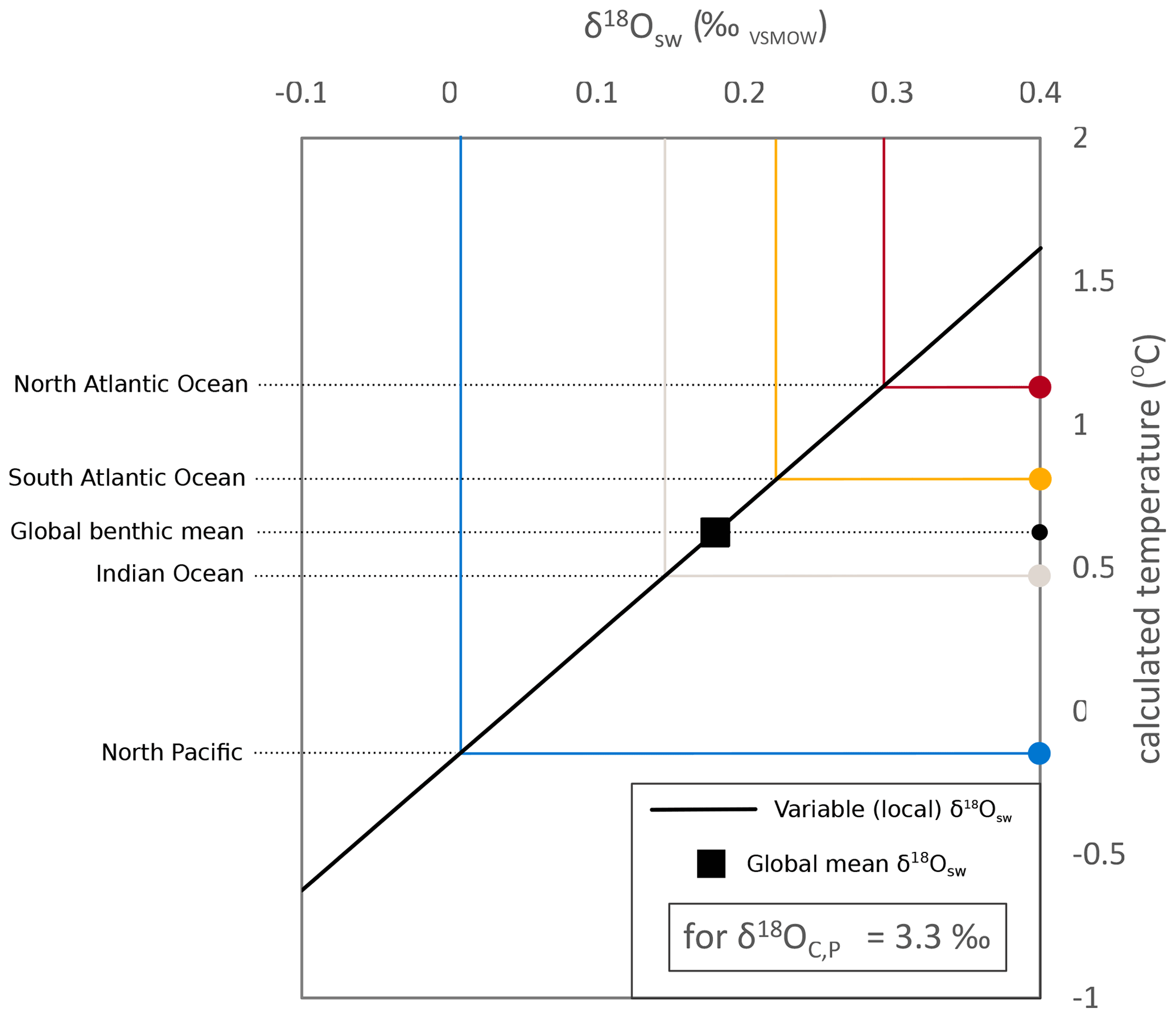
Figure A1 Example palaeotemperature calculation of Marchitto et al. (2014) for a δ¹⁸O_{Cibicidoides, Planulina} of 3.3 ‰ with a variable δ¹⁸O_sw. The calculated temperature using the global mean δ¹⁸O_sw from Cramer et al. (2011) for the Holocene is marked, and selected ocean region mean δ¹⁸O_sw values have been labelled on the figure (values evident in Fig. A2 for ocean basin means). When applying a local correction to δ¹⁸O_sw, the North Atlantic calculated temperature is ∼0.5 ^∘C warmer, and the North Pacific calculated temperature is ∼0.7 ^∘C cooler, than the when applying the global mean δ¹⁸O_sw.

The seawater δ¹⁸O_sw is determined by global ice volume (which we get from Cramer et al., 2011), local temperature, and local salinity (Rohling, 2013). In the present day, with an active AMOC, the North Atlantic benthos have a more positive δ¹⁸O_sw than, for example, the North Pacific. This is due to both temperature and salinity, with the salty North Atlantic waters transported to the deep by the AMOC. In our model ensembles, the benthic salinity is affected by both CO₂ and flux correction, as these affect ocean circulation. Therefore, for each simulation, we apply a δ¹⁸O_sw-driven correction to the palaeotemperatures due to their locally modelled salinity. To do this, we use present-day deep-water (2500 m) δ¹⁸O_sw (LeGrande and Schmidt, 2006) and salinity (WOA 2013; Zweng et al., 2013) to create a general linear model (Eq. A1):

$$\begin{array}{}\text{(A1)}& {\mathit{\delta }}^{\mathrm{18}}{\mathrm{O}}_{\text{sw}}=\mathrm{0.8}S-\mathrm{27.7},\end{array}$$

where S is salinity.

The North Atlantic is the region that is most affected by changes in salinity; therefore, the greatest temperature offset will be in this location. We adjusted the salinity model to get best fit values for the North Atlantic as well as a good fit for the difference in δ¹⁸O_sw between the North Atlantic and the Pacific. All ocean locations with δ¹⁸O_sw between −0.3 ‰ and 0.3 ‰ are shown in a cross plot of data and salinity-model-derived δ¹⁸O_sw in Fig. A3. The grouping of points clearly offset from the 1:1 line are the high southern latitudes (also clearly visible in Fig. A2). The accuracy of the salinity model in finding δ¹⁸O_sw is ±0.03 ‰ at 1 standard deviation and ±0.06 ‰ at the 95 % confidence level excluding latitudes higher than 70^∘ (where we have no foraminifera shell δ¹⁸O data points in any case).

The palaeotemperature equation that we apply is the linear model from Marchitto et al. (2014, Eq. 8 therein), using the global ice volume estimate from Cramer et al. (2011). The δ¹⁸O_sw model from salinity is also linear, so we apply a simple linear correction to the calculated temperature (Table S2). To obtain the δ¹⁸O_sw offset, we first find the modelled global mean salinity (not including latitudes higher than 70^∘) and then subtract it from the modelled benthic salinity, giving a ΔS field (an offset from the mean). We apply Eq. (A2) to find ΔT, where 0.8 is the gradient of the linear δ¹⁸O_sw model (Eq. A1), and 0.224 is the gradient of the linear palaeotemperature model (Marchitto et al., 2014), and we use this to correct T for salinity. The uncertainty for the temperature correction is ±0.13 ^∘C at 1 standard deviation and 0.23 ^∘C at the 95 % confidence level (based on the δ¹⁸O model uncertainties). The range of temperature correction corresponding to the benthic δ¹⁸O_sw spread (of ∼0.4 ‰) in the present day is 1.8 ^∘C.

$$\begin{array}{}\text{(A2)}& \mathrm{\Delta }T={\displaystyle \frac{\mathrm{0.8}\mathrm{\Delta }S}{\mathrm{0.224}}}\end{array}$$

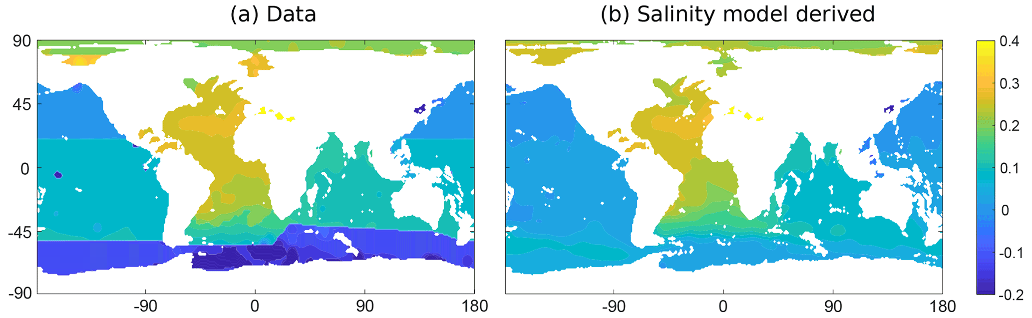
Figure A2 δ¹⁸O_sw data from LeGrande and Schmidt (2006) at 2500 m depth (at depths below 2500 m, the data set shows little change in δ¹⁸O_sw compared with the values shown) (a) and salinity-derived δ¹⁸O_sw (b), where salinity data from WOA 2013 (Zweng et al., 2013) are used in the model in Eq. (A1) (all in ‰_VSMOW).

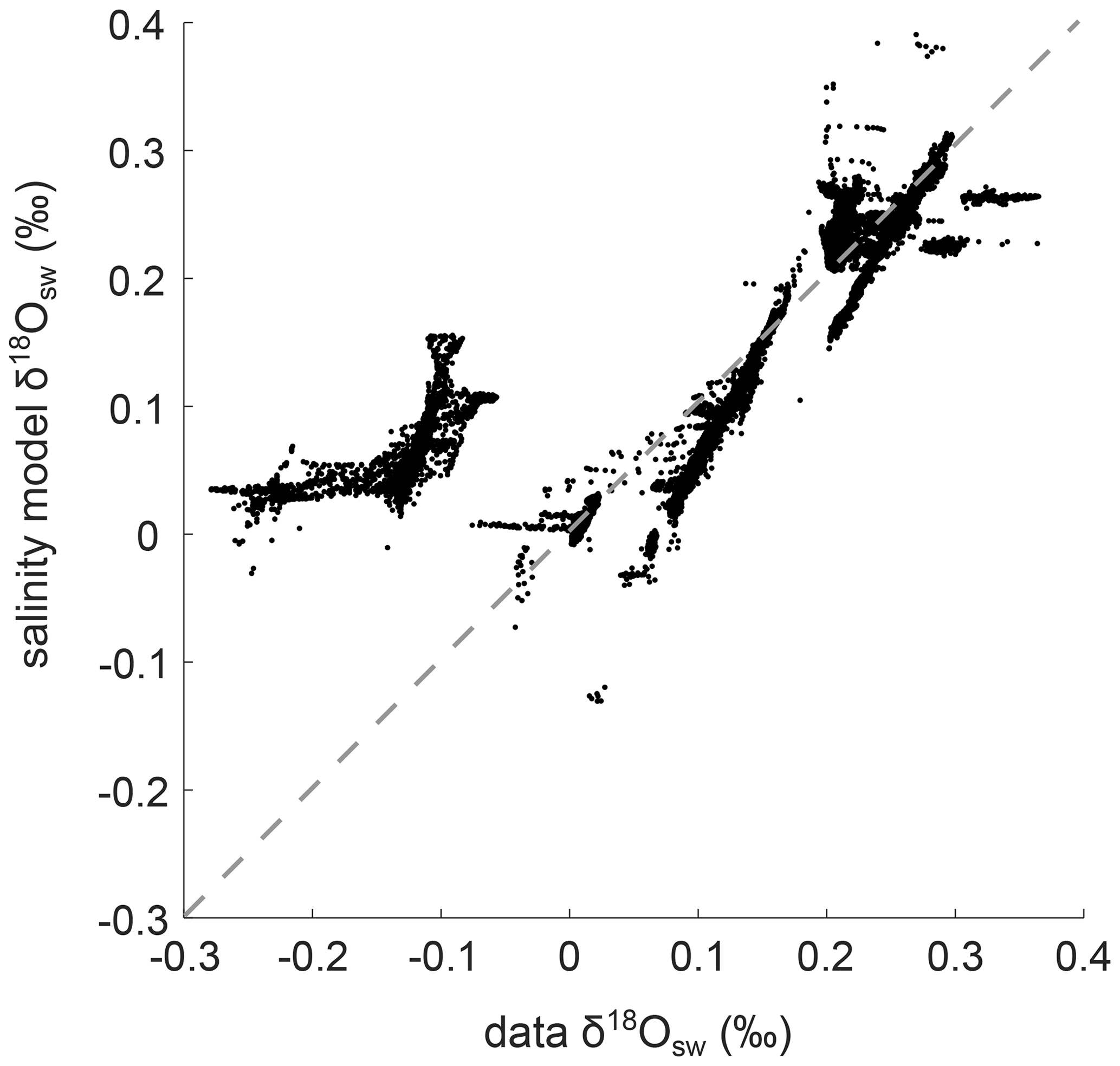
Figure A3 Cross plot of data δ¹⁸O_sw and salinity-model-derived δ¹⁸O_sw as shown in Fig. A2. The offset region (where data shows low δ¹⁸O_sw compared with the derived salinity model) is the Southern Ocean, where the polar front more strongly affects ocean water δ¹⁸O_sw than salinity/thermohaline circulation.

Appendix B: Model boundary conditions

In this paper, as per previous (deeper time) palaeo-applications of the cGENIE.muffin model (e.g. Ridgwell and Schmidt, 2010), we derive the required boundary conditions from a representative fully coupled GCM experiment using the “muffingen” open-source software version v0.9.20 (which is assigned the following DOI: https://doi.org/10.5281/zenodo.4615664), rather than using observations. This software takes a specific GCM experiment as input and carries out the following:

1. It creates output (here, 36×36 with 16 levels in the ocean) grids.

2. Using (1), it derives a land–sea mask and ocean bathymetry on the output grid. The land–sea mask is filtered to prevent the occurrence of isolated inland seas and single-cell-width coastal embayment, while the ocean bathymetry is filtered to avoid single-cell “holes” occurring in the ocean floor.

3. The model then generates drainage basins determining where precipitation is directed towards the ocean (and, hence, runoff direction). The specific scheme used here is known as a “roofing scheme” and operates to create a watershed approximately equidistant from the coast.

4. It next derives island and ocean path files required by the ocean circulation model.

5. The model then re-grids GCM wind stress and (10 m) wind velocity to the output grid (for wind stress, this means re-gridding to both u- and v-edge grids). Wind speed is calculated from the mean annual wind velocity components.

6. Finally, it re-grids the GCM planetary albedo and converts to a zonally averaged profile.

The GCM simulations underlying our cGENIE model configurations were carried out using HadCM3LM2.1aE, which is described in detail in Valdes et al. (2017). The models are constrained with palaeogeographies and a solar constant appropriate for each geological stage in the Miocene as well as a CO₂ mixing ratio of 400 ppmv. The experimental design is described in detail in Farnsworth et al. (2019). The specific GCM experiments that we used from Farnsworth et al. (2019) are those for the Holocene (0 Ma), Piacenzian (2.58–3.6 Ma), Zanclean (3.6–5.333 Ma), Messinian (5.333–7.246 Ma), Tortonian (7.246–11.63 Ma), Serravallian (11.63–13.82 Ma), and Langhian (13.82–15.97 Ma); we simplified and adopted these experiments to approximately evenly spaced slices at 0.0, 2.5, 4.5, 7.5, 10.0, 12.5, and 15.0 Ma (Table 1 main text).

For all time-slice configurations we generally follow the default re-gridding algorithm of the muffingen software in order to avoid imposing prior assumptions regarding the importance of specific ocean features, meaning that a Mediterranean Sea is not present for most of the reconstructed continental configurations in cGENIE. Only in the 12.5 and 15.0 Ma time slices is the remnant Tethys Ocean sufficiently expansive to re-grid as an ocean basin at the selected 36×36 (16 levels) model resolution. We do, however, make the following manual interventions in the generation of the land–sea mask (but not in ocean bathymetry):

• for 0 Ma (late Holocene), the Panama Isthmus as well as the tip of South America is made continuous;

• for 10.0, 12.5, and 15.0 Ma, the Arctic is opened up (turning land cells to ocean) in order to approximately preserve the global land fraction of 0.29 in the underlying GCM across all seven reconstructions;

• in a second set of simulations, the Panama Isthmus is made continuous for the 10 to 2.5 Ma time slices and the late-Holocene Panama Isthmus is left open.

The resulting cGENIE bathymetry for each time slice is shown in Fig. 3. The Drake Passage is already open at 15 Ma, but it widens by 12.5 Ma and gradually deepens. The Atlantic Ocean widens and deepens throughout, and the Pacific generally deepens. The Australian land mass moves north, and the Indonesian seaway gradually reduces. Africa moves north, reducing the Tethys Sea area, which is already closed off from the Indian Ocean at 15 Ma. The Tethys disappears by 10 Ma, and the Mediterranean Sea is not included in the simulations. Greenland is isolated from North America until 7.5 Ma, and the Bering Strait is closed until 7.5 Ma. Only at the Holocene is the Bering Strait open and is Greenland once again isolated from North America, allowing mixing between the Arctic Ocean, the North Pacific, and North Atlantic at the same time.

We chose and calculate a zonally average (GCM-derived) planetary albedo profile (rather than a 2D re-gridded one) in order to retain closer back-compatibility with the original GENIE configuration in which an idealised zonal profile is applied (e.g. Edwards and Marsh, 2005). Different GCMs average and save wind speed differently (or only as velocity vectors), meaning that the final re-gridded wind speed product can differ substantially between GCMs and with modern observations. Because of this, we re-scale air–sea gas exchange in the late-Holocene configuration in order to give a mean global and annual average modern air–sea coefficient value for CO₂ of approximately 0.058 $\mathrm{mol}{\mathrm{m}}^{-\mathrm{2}}{\mathrm{yr}}^{-\mathrm{1}}\mathrm{\mu }{\mathrm{atm}}^{-\mathrm{1}}$. This same air–sea gas exchange scaling is then applied to all older time slices. As compared to Cao et al. (2009), we also forego the high southern latitude zone of reduced atmospheric diffusivity, previously used for present-day model configurations (described further in Marsh et al., 2011). Initial mean salinity was reduced by 1 to 33.9 PSU in all time-slice configurations for simplicity and consistency (although we recognise that mean ocean salinity should realistically progressively decrease from a modern value of 34.9 back in time with progressively decreasing global land ice volume). The orbital configuration was kept at its modern settings throughout all time slices (0.0167 eccentricity, 0.397789 for sine of obliquity, and 102.92 for the longitude of perihelion; longitude is in degrees). However, we did vary the following model parameter values and initial conditions as a function of (geological) time (time-slice age):

• The solar constant is assumed to change with time and to follow Gough (1981) (see also Feulner, 2012), resulting in a small increase between 15.0 and 0 Ma, from 1366.09 W m⁻² (a reduction of 0.14 % compared to modern) at 15.0 Ma to 1368.0 W m⁻² by the late Holocene.

• The mean Mg$/$Ca ratio of the ocean is also assumed to change with time, following Tyrrell and Zeebe (2004). The corresponding range is then from 13.15 $\mathrm{mmol}{\mathrm{kg}}^{-\mathrm{1}}{\mathrm{Ca}}^{\mathrm{2}+}$ and 41.21 $\mathrm{mmol}{\mathrm{kg}}^{-\mathrm{1}}{\mathrm{Mg}}^{\mathrm{2}+}$ at 15.0 Ma to 10.28 $\mathrm{mmol}{\mathrm{kg}}^{-\mathrm{1}}{\mathrm{Ca}}^{\mathrm{2}+}$ and 52.81 $\mathrm{mmol}{\mathrm{kg}}^{-\mathrm{1}}{\mathrm{Mg}}^{\mathrm{2}+}$ in the present-day ocean. (Changing ocean Mg$/$Ca with time influences the calculation of carbonate saturation as well as dissociated constants.)

All boundary configurations and relevant parameter settings (as well as the cGENIE.muffin model code itself) are open-source. Refer to our “Code availability” statement for information regarding obtaining and running any or all of these model configurations.

Figure B1 Comparison of PLATES-derived rotation (applied to the full data set) to the HadCM3 rotation (used as a basis for the cGENIE model). The mean difference between PLATES and HadCM3 palaeo-locations for latitude is 0.216^∘ (standard deviation of 1.14^∘), whereas for longitude, the mean difference is −0.498^∘ (standard deviation of 1.80^∘).

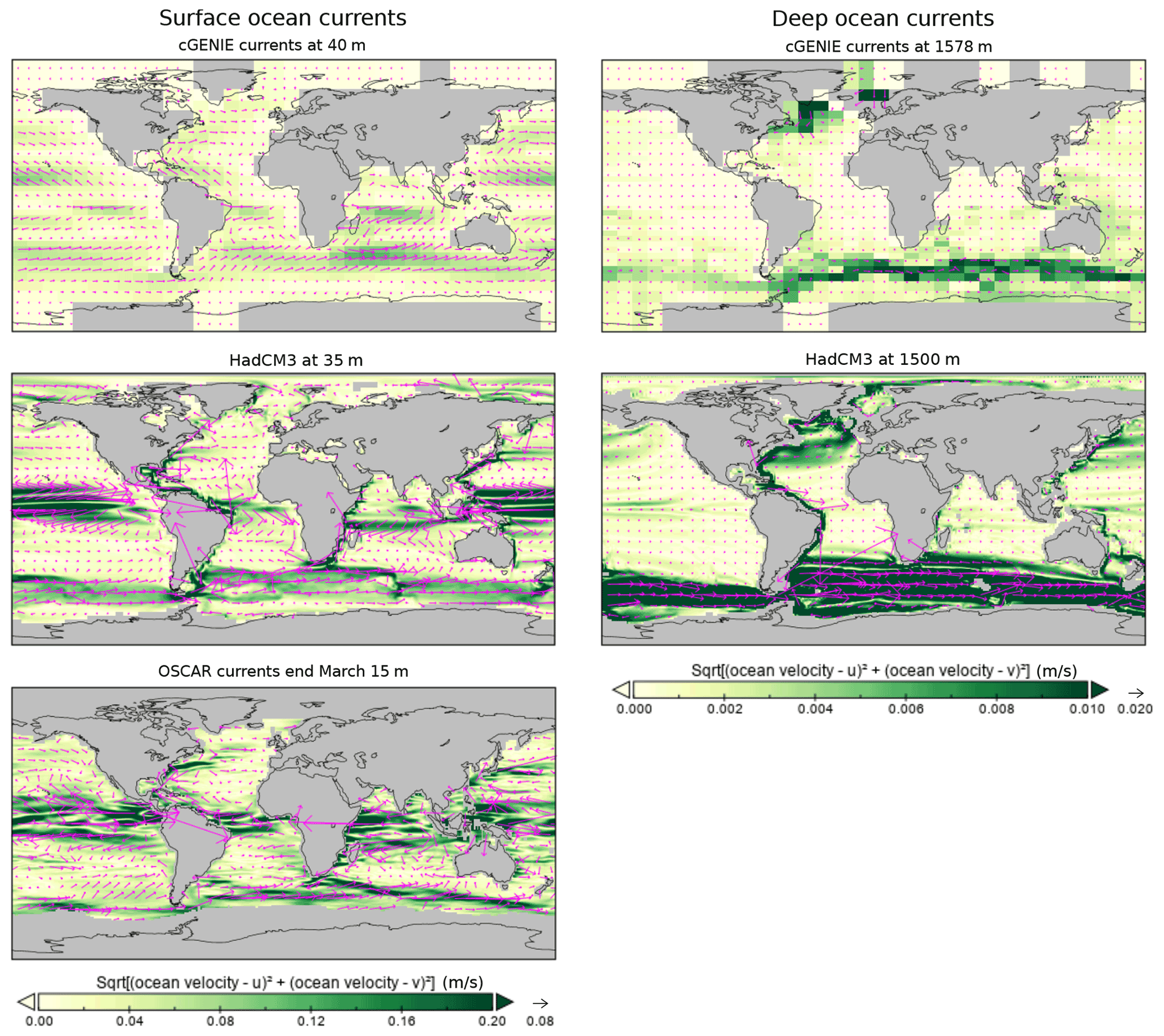
Figure B2 Comparison of cGENIE to HadCM3 near-surface and deep-ocean currents and to data-indicated near-surface currents from OSCAR (Ocean Surface Current Analysis in Real-time) (ESR, 2009). Note the scale difference for the surface and deep-ocean colour bars and vectors.

Figure B3 Location of salinity addition and salinity removal common to all configurations for the salinity flux adjustment controller “FwF”.

Appendix C: Sustained climate oscillations in the ensemble

The settings for which sustained climate oscillations were identified are shown in Fig. C1. These oscillations were present in a subset of ensemble members in all time-slice ensembles except the Holocene, and they were more prevalent for the open-CAS configurations. They ranged in amplitude from 0.3 to 2.5 ^∘C in benthic temperature with periods of 1.7 to 4.5 kyr.

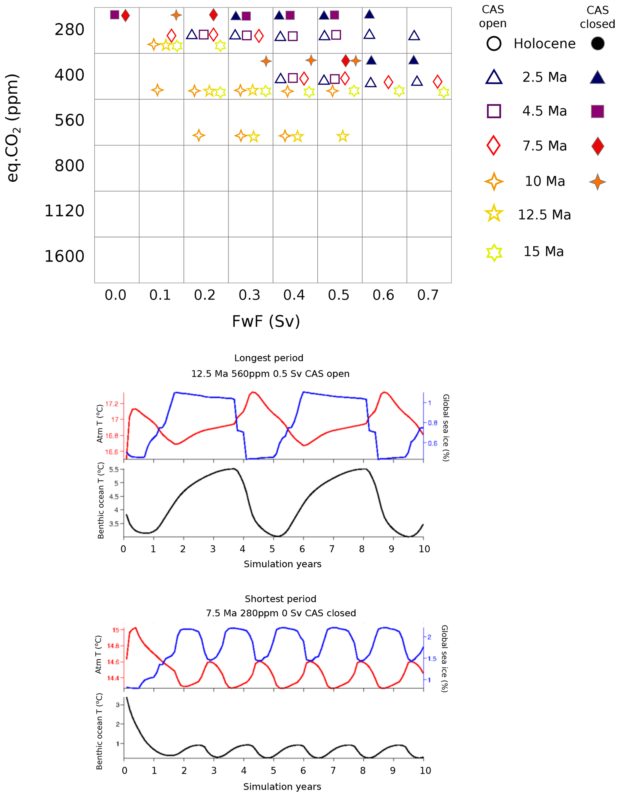
Figure C1 Ensemble settings that displayed sustained oscillations in benthic ocean temperature (top). Model output for atmospheric temperature, sea ice, and benthic temperature for the longest- and shortest-period oscillations (bottom panels).

Appendix D: Details on selecting the “best fit” settings

D1 Holocene, 0 Ma

For the Holocene slice, we have a priori knowledge that CO₂ during this warm interglacial period was around 280 ppm (Indermühle et al., 1999) – a value which in cGENIE agrees with the surface ocean temperature data. This gives us some confidence in the cGENIE Earth system model and the methodology; however, although we use a new and different GCM-derived (Farnsworth et al., 2019) modern continental configuration here, cGENIE has already been calibrated against present-day observed ocean temperatures at an atmospheric CO₂ value of ca. 280 ppm (e.g. Price et al., 2009; Ridgwell et al., 2007), so an acceptable fit to SSTs for an eq.CO₂ value of 280 ppm is not necessarily unexpected. The global benthic temperature estimate from Cramer et al. (2011) represents a mean climate for both glacial and interglacials, which is around 2 ^∘C cooler than the warmer Holocene. For a global benthic temperature that is 2 ^∘C warmer than that from Cramer et al. (2011), a relatively low flux correction of 0.1 to 0.2 Sv is required to fit the data (in comparison, the present-day calibrated value in cGENIE is 0.32 Sv). However, the benthic δ¹³C data constraints (Fig. 6) tend towards a higher M-score for a higher flux correction, so we chose a best fit value of FwF 0.2 Sv for the closed-CAS case. In an open-CAS case, the δ¹³C constraint suggests a higher FwF, so the open-CAS best fit is set at 0.3 Sv.

D2 Piacenzian, 2.5 Ma

For the 2.5 Ma slice, surface and benthic temperatures both suggest a higher (and larger range for a fit to) eq.CO₂ than for the Holocene, so 400 ppm is selected as the best fit eq.CO₂ value (although 280 ppm would also work well). Similar to the Holocene, a higher flux correction (FwF) at 2.5 Ma tends to show a better model–data benthic δ¹³C agreement for the open-CAS case, although this constraint is less strong than the benthic temperature constraint (maximum M-score for benthic temperature is ∼0.4, whereas it is ∼0.2 for δ¹³C at 0.5 Sv). Hence, for the open CAS, we select 0.3 Sv as the FwF value, which is at the higher end of the benthic temperature (δ¹⁸O-derived) data set but is in agreement with global mean benthic temperature from Cramer et al. (2011). The closed CAS shows a generally cooler benthic ocean temperature and a lower FwF, so an eq.CO₂ value of 400 ppm is combined with a FwF of 0.1 Sv for the closed CAS.

D3 Zanclean, 4.5 Ma

At 4.5 Ma, the surface temperature data support an even higher eq.CO₂ value in cGENIE, but here the δ¹³C constraint is stronger (compared with that at 2.5 Ma) for both CAS cases (and instead supports a lower CO₂ and higher FwF) as the M-score increases in this direction of parameter space (Fig. 6). Hence, we place the best fit in this direction for the open CAS, with an eq.CO₂ value of 400 ppm and an FwF value of 0.5 Sv. For the closed CAS, the benthic δ¹³C constraint is stronger still, and, together with a benthic temperature constraint indicating a lower FwF than for the open CAS, an eq.CO₂ of 400 ppm is combined with a FwF of 0.2 Sv for the closed CAS.

D4 Messinian, 7.5 Ma

At 7.5 Ma, surface temperature data require a significantly increased eq.CO₂ compared with 4.5 Ma, with 800 ppm clearly being the best fit CO₂ value. A similar tendency (to 4.5 Ma) toward lower CO₂ but higher FwF is also apparent in the δ¹³C constraint for this time slice, although at 800 ppm, this is less strong (with a low M-score for the δ¹³C constraint at 800 ppm and high FwF). Again, with a closed CAS, the benthic temperature constraints indicate lower FwF than for the open CAS. The flux correction is set at 0.4 Sv, which is near the centre of the benthic temperature maximum M-score (shown as a dashed blue contour in Fig. 6) for the open-CAS case. For the closed-CAS case, 800 ppm is combined with an FwF of 0.3 Sv, which is towards the higher end of the benthic temperature constraint, but in the direction of increasing δ¹³C M-score.

D5 Tortonian, 10 Ma

For 10 Ma and older time slices, the model–data M-score for surface temperature declines, although with higher scores for higher CO₂ in all three cases. At 10 Ma, for open CAS, the benthic (δ¹⁸O) temperature data set suggests a CO₂ of 800 ppm and an FwF of 0.3 to 0.4 Sv. The δ¹³C fit surface tends towards higher M-score values for higher flux, so we set FwF at 0.4 Sv for open CAS. For closed CAS, both benthic constraints suggest a lower FwF, so 800 ppm combined with an FwF of 0.3 Sv is selected for closed CAS.

D6 Serravallian, 12.5 Ma

The 12.5 Ma slice seems to show a transition state for the trends in δ¹³C, with an overall low M-score for all combinations of CO₂ and FwF. As δ¹³C provides a weak constraint, the CO₂ and FwF values are selected as 1120 ppm and 0.2 Sv respectively as a compromise between the high-CO₂ requirement for surface temperature and the lower-CO₂–higher-FwF for the benthic temperature.

D7 Langhian, 15 Ma

At 15 Ma, the ensemble surface of the M-score for δ¹³C is inversed compared with other time slices, showing a higher score for (generally) higher eq.CO₂ combined with a lower FwF. Although we have fewer surface temperature data points, they suggest a high eq.CO₂, which is somewhat in disagreement with the benthic temperature data set that favours a mid-range eq.CO₂ and a higher FwF. As the δ¹³C constraint tends towards a lower FwF (compared with time slices younger than 10 Ma), we select an eq.CO₂ value of 1120 ppm and a low flux correction of 0.1 Sv.