the Creative Commons Attribution 4.0 License.
the Creative Commons Attribution 4.0 License.
 | 21 Sep 2021
FYRE Climate: a high-resolution reanalysis of daily precipitation and temperature in France from 1871 to 2012
Alexandre Devers
Jean-Philippe Vidal
Claire Lauvernet
Olivier Vannier
Surface observations are usually too few and far between to properly assess multidecadal variations at the local scale and characterize historical local extreme events at the same time. A data assimilation scheme has been recently presented to assimilate daily observations of temperature and precipitation into downscaled reconstructions from a global extended reanalysis through an Ensemble Kalman fitting approach and to derive high-resolution fields. Recent studies also showed that assimilating observations at high temporal resolution does not guarantee correct multidecadal variations. The current paper thus proposes (1) to apply the data assimilation scheme over France and over the 1871–2012 period based on the SCOPE Climate reconstructions background dataset and all available daily historical surface observations of temperature and precipitation, (2) to develop an assimilation scheme at the yearly timescale and to apply it over the same period and lastly, (3) to derive the FYRE Climate reanalysis, a 25-member ensemble hybrid dataset resulting from the daily and yearly assimilation schemes, spanning the whole 1871–2012 period at a daily and 8 km resolution over France. Assimilating daily observations only allows reconstructing accurately daily characteristics, but fails in reproducing robust multidecadal variations when compared to independent datasets. Combining the daily and yearly assimilation schemes, FYRE Climate clearly performs better than the SCOPE Climate background in terms of bias, error, and correlation, but also better than the Safran reference surface reanalysis over France available from 1958 onward only. FYRE Climate also succeeds in reconstructing both local extreme events and multidecadal variability. It is freely available at https://doi.org/10.5281/zenodo.4005573 (precipitation, Devers et al., 2020b) and https://doi.org/10.5281/zenodo.4006472 (temperature, Devers et al., 2020c).
- Article
(8030 KB) - Full-text XML
- BibTeX
- EndNote


Several studies show that long-term meteorological observation often displays strong multidecadal variations both in terms of annual values (Slonosky, 2002) and extremes (Willems, 2013). These variations in meteorological variables end up affecting multidecadal variations of streamflow observations (Boé and Habets, 2014). However, the few available long-term observations do not allow us to grasp the evolving climate in a spatially continuous way. To solve this discontinuity issue, daily meteorological high-resolution surface reanalyses have been built at the country scale (Vidal et al., 2010a; Quintana-Segui et al., 2017) or spanning Europe (Landelius et al., 2016; Soci et al., 2016). These reanalyses are mainly built using optimal interpolation (Gandin, 1965) combining daily observations and large-scale atmospheric reanalyses as background. However, due to the low number of daily meteorological observations before the 1950s (Caillouet et al., 2019), these reanalyses are usually limited to the second half of the 20th century (Minvielle et al., 2015). This lack of sufficient daily historical observations in many countries in Europe led to the creation of several long-term high-resolution reconstructions. These datasets are mainly built using statistical downscaling of global atmospheric reanalyses (Dayon et al., 2015; Minvielle et al., 2015; Caillouet et al., 2019; Horton and Brönnimann, 2018), but in data rich areas, some are also built as an interpolation of surface observations (Keller et al., 2015).
In the past few years, some studies have also developed or used different processes to take advantage of both historical observations and downscaled reconstructions. For instance, the downscaled reconstructions may be modified using individual long-term observed time series (Kuentz et al., 2015; Brigode et al., 2016). Observations may also be integrated in a postprocessing of the downscaling step, e.g., through the selection of a unique member from a downscaled ensemble (Bonnet et al., 2017, 2020; Minvielle et al., 2015).
In parallel, paleoclimate studies that usually deal with coarser temporal and spatial resolutions have used data assimilation (DA) to reconstruct past climate fields. DA usually combines (i) a background, (ii) observations, (iii) a model, and (iv) the associated uncertainty in providing an optimal analysis and its associated error (Asch et al., 2016). DA is usually composed of two steps: the analysis and the forecast, which is a propagation of the analysis by the (dynamical) model. In paleoclimate studies in which the propagation step may be typically highly computationally demanding, DA methods have been applied “offline” (Goosse et al., 2006; Annan and Hargreaves, 2012; Bhend et al., 2012; Hakim et al., 2016; Valler et al., 2019): the background is computed by the dynamical model once for the entire period, and the DA comes down to the analysis step (Matsikaris et al., 2015).
Some recent studies have also attempted to follow the offline DA methodology at higher resolution to assimilate daily observations into various reconstructions. Pfister et al. (2020) have assimilated daily temperature over Switzerland into a statistical reconstruction, leading to an improvement using only a limited number of stations – 25 over all of Switzerland. Devers et al. (2020a) also developed a DA scheme of daily precipitation and temperature over France into the SCOPE Climate (Spatially COherent Probabilistic Extension Method) downscaled reconstruction dataset (Caillouet et al., 2019). The DA method is an offline Ensemble Kalman Filter (Evensen, 2003), also referred to as Ensemble Kalman fitting (EnKf, Bhend et al., 2012). They showed that the DA scheme allows for improvements upon the background even with a limited number of assimilated stations. However, assimilating observations at a high temporal resolution as in the two previous examples does not guarantee a correct multidecadal variation in the reanalysis (Steiger and Hakim, 2016). To bypass this problem, some studies in paleoclimatology assimilate temporal averages of observations through offline DA in existing reconstructions (Steiger and Hakim, 2016; Dirren and Hakim, 2005; Huntley and Hakim, 2010; Steiger et al., 2014).
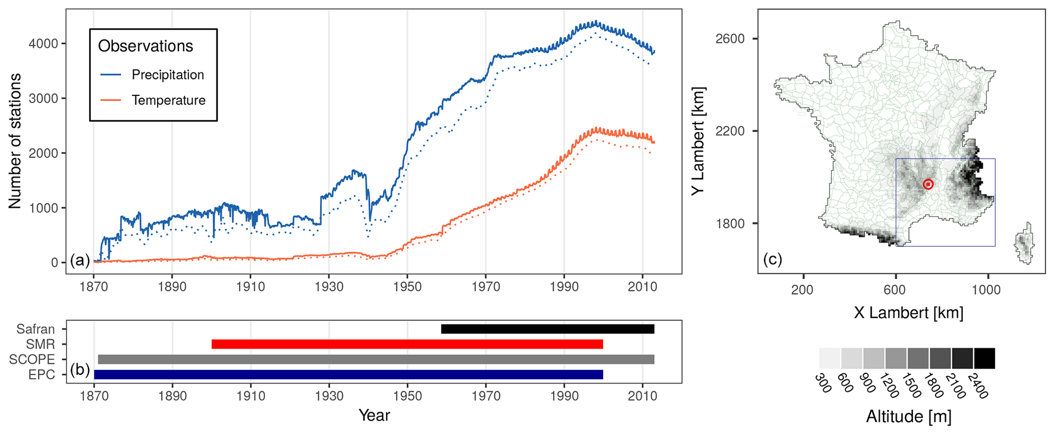
Figure 1(a) Availability of meteorological observations in the Météo-France database over the 1871–2012 period. Full lines represent the number of open stations during the considered year and dotted lines represent the number of stations with a complete series. (b) Availability of the different gridded datasets: SCOPE Climate, Safran, European pattern climatology, and monthly homogenized series. (c) Map of the 608 climatologically homogeneous zones – in green – as defined in Safran, and altitude of the 8 km grid cells of SCOPE Climate and Safran. The case study cell (id: 7548), highlighted in red, is located in the Cevennes area at the altitude of 1165 m a.s.l. in a mountainous Mediterranean climate. An observation station (id: 7154005, Mazan-l'Abbaye) is located in this cell at the altitude of 1240 m a.s.l. The blue frame represents the study area for the heavy rainfall event of 21 September 1890 (see Sect. 4.5).
Devers et al. (2020a) developed and tested their ensemble DA scheme over a short period of time (2009–2012) with assimilated observation density reproducing the historical density (number and spatial patterns) at a few carefully selected years between 1871 and 2012, representative of the evolution of the observation network: 1871, 1900, 1930, and 1950 (see Fig. 1a, for the evolution of the number of available observations). Such a setup allowed for keeping a large number of independent observations – 783 for precipitation and 1500 for temperature – for validation purposes. The authors showed that the ensemble produced is well calibrated, and that the performance of the reanalysis decreases when the density of assimilated observations decreases, i.e., when one goes further back in time. Over the 2009–2012 period, the DA scheme furthermore leads to a better performance than the current reference surface reanalysis over France (Safran, which assimilates all available observations Vidal et al., 2010b), for (1) temperature even with an assimilated density as low as that of 1871, and (2) for precipitation with a density as low as that of 1930. Note that assessing the DA scheme against independent observations as done by Devers et al. (2020a) is a prerequisite to the current study, which uses all available observations.
Indeed, this study applies the scheme developed by Devers et al. (2020a) over the 1871–2012 period in order to produce the full FYRE Daily reanalysis, composed of 25 members of daily precipitation and temperature at a 8 km resolution over France. In order to address multidecadal variations, a new DA scheme at the yearly timescale is then proposed once again using SCOPE Climate (Caillouet et al., 2019) as a background. The scheme is then applied over the 1871–2012 period for both precipitation and temperature leading to the 25-member yearly reanalysis of precipitation and temperature at 8 km resolution: FYRE Yearly. In order to include both multidecadal variations and extreme events, FYRE Daily and FYRE Yearly are hybridized to build a new reanalysis: FYRE Climate. Finally, the benefits of hybridization is assessed by comparing FYRE Daily and FYRE Climate against several products over a recent period (1950–2000) and over the entire 20th century. These comparisons include the computation of several metrics: continuous ranked probability score (CRPS, Brown, 1974), bias, error, and correlation. The multidecadal variations of the two reanalyses and the background are also compared with those of other products. Furthermore, the reconstruction of extreme events is investigated using the study of an extreme rainfall event during September 1890 and the unusually cold month of December 1879.
The paper is organized as follows: Sect. 2 introduces the background, the assimilated observations and their metadata, as well as validation datasets. Section 3 describes the DA implementation and the creation of the different reanalyses. Their validation through different comparisons and examples is presented in Sect. 4. Finally, several points are discussed in Sect. 5 and conclusions are drawn in Sect. 6.
2.1 Background
The SCOPE (Spatially COherent Probabilistic Extension Method, Caillouet et al., 2016, 2017) climate downscaling method is based on the analog approach, which assumes that similar large-scale patterns of atmospheric circulation lead to similar local meteorological conditions of, e.g., temperature and precipitation (Lorenz, 1969). SCOPE uses an ensemble analog approach to reconstruct high-resolution climate fields from large-scale information on atmospheric circulation. SCOPE draws on several works on climate downscaling with analogs (Radanovics et al., 2013; Ben Daoud et al., 2016; Caillouet et al., 2016, 2017), and the reader may refer to these for more details. In short, based on information on large-scale atmospheric circulation from, e.g., a global reanalysis, SCOPE generates an ensemble of high-resolution daily meteorological fields through a resampling of an archive of such fields. Note that the resulting fields from each ensemble member are coherent in space as well as across variables, thanks to the use of the Schaake Shuffle (Clark et al., 2004).
The application of the SCOPE method using the ensemble mean values of the Twentieth Century Reanalysis (Compo et al., 2011) as a source of large-scale information – predictors – and the Safran reanalysis (Vidal et al., 2010b) as an archive for analogs – predictands – has led to the creation of the SCOPE Climate dataset (Caillouet et al., 2019). This daily 25-member ensemble reconstruction is available on a 8 km grid (see Fig. 1) over the 1871–2012 period for precipitation (Caillouet et al., 2018a), temperature (Caillouet et al., 2018b), and Penman-Monteith reference evapotranspiration (Caillouet et al., 2018c). Note that as SCOPE Climate resamples Safran data, the daily temperature is actually computed as the daily average of hourly temperature.
The comparison of SCOPE Climate with the independent Météo-France long-term homogenized series (Moisselin et al., 2002, see Sect. 2.4.2 for details about this dataset) has put forward a low and steady error – at the monthly timescale – over the whole 20th century (Caillouet et al., 2019).
Two background ensembles were extracted from SCOPE Climate for this study:
-
for daily DA, the 25-member ensemble of daily values of temperature and precipitation from SCOPE Climate;
-
for yearly DA, the 25-member ensemble of yearly-average temperature and the yearly-accumulated precipitation from SCOPE Climate.
In both cases, data were extracted between 1 January 1871 and 29 December 2012, i.e the entire period of availability of SCOPE Climate. 2012 yearly values are computed over the available period.
2.2 Assimilated observations
Surface observations originate from the Météo-France database composed of the daily sum of precipitation, and daily minimum and maximum temperature. The observation network has evolved from less than 10 stations of temperature and precipitation in the 1870s to more than 2500 stations for temperature and 4300 for precipitation at the end of the 20th century (Fig. 1a). The number of stations with a full year of available data evolved in parallel. This large number of observations is partially based on a strong voluntary observation network in France (Galliot, 2003; Capel, 2009).
Variables used as observations over the 1871–2012 period are
-
for daily DA: the daily sum of precipitation and the daily mean temperature;
-
for yearly DA: the yearly sum of precipitation and yearly mean temperature for stations with a full year of available data. Values are otherwise discarded and not used in the yearly DA.
Note that because of the low availability of hourly measurements in the past, the daily mean temperature is computed here as the mean of the daily maximum temperature and the daily minimum temperature. Observed yearly values for 2012 are computed between 1 January and 29 December to stick to the background data availability.
2.3 Metadata for observations
Along with observed values, some metadata are available over the 1871–2012 period. Three types of metadata have been used in this study in order to best define the measurement error of temperature and precipitation.
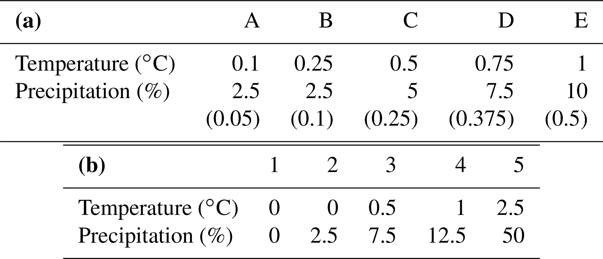
The first type of metadata available over the entire period is the type of station, ranging from 0 for the highest quality to 5 for the lowest quality. This classification is not linked to any numerical values of measurement error but can be used as an indicator of the overall quality of the station. The second type of metadata, noted σMP, is only available from 1999 onward and represents the maintained performance of each station (Table 1a; Leroy, 2010). This classification includes the intrinsic quality of the measurement device and the quality of the measurement method. Lastly, the site representativeness, noted σSR, is also available over the 1999–2012 period (Table 1b; Leroy and Lèches, 2014). This classification takes into account the error due to the influence of the nearby environment of the station. The maintained performance and site representativeness give information about the daily error measurement and are related to the station quality as established by Météo-France and the World Meteorological Organization (WMO, 2014).
Table 1Station classifications and related measurement uncertainty – standard deviation, computed as half of the 95 % confidence interval – for daily temperature and daily precipitation. (a) Maintained performance (Leroy, 2010). The standard deviation for precipitation is selected as the maximum between the percentage value and the minimum value indicated in brackets (in mm). (b) Representativeness of the site (Leroy and Lèches, 2014).
2.4 Other datasets
2.4.1 Safran
The Safran system is an analysis system based on an optimal interpolation scheme that merges in situ observation (temperature, precipitation, relative humidity, wind speed, and cloudiness) and a background – ERA-40 large-scale reanalysis (Uppala et al., 2005) and ECMWF operational analyses, or climatological values (for precipitation). The analysis is performed on 608 climatologically homogeneous zones (see Fig. 1c) and is afterwards disaggregated onto 8602 cells in France (8 km grid) based only on altitude (Quintana-Segui et al., 2008). The Safran reanalysis is available from 1 August 1958 onwards and is updated annually (Vidal et al., 2010b). In this study, daily precipitation and daily temperature – computed as the average of hourly values – are extracted from the Safran database over the 1 January 1958–29 December 2012 period. The Safran reanalysis is used here to assess features of the background and the different reanalyses over the last 50 years or so.
2.4.2 Monthly homogenized series (SMR)
The monthly homogenized series – called SMR for “Séries Mensuelles de Référence” – are produced by Météo-France. The homogenization is intended to detect and correct potential homogeneity breaks related to changes in location or instrumentation (Moisselin et al., 2002; Gibelin et al., 2014). SMR comprise two different datasets:
-
1583 time series for precipitation and 308 for temperature allowing for the capture of the spatial patterns over France but only covering the period 1959–2009 (Gibelin et al., 2014);
-
332 time series for precipitation and 88 for temperature covering the period 1900–2000 (Moisselin et al., 2002). Although stations are not distributed in a homogeneous way over France, these series constitute a reliable reference for analyzing multidecadal variations as well as long-term trends.
The SMR is a high-quality dataset that will be used to assess the quality of the background and several reanalyses in terms of multidecadal variations and trends, but also to evaluate their quality at the monthly timescale through different metrics – bias, correlation, and error – over different periods.
2.4.3 European pattern climatology
The monthly gridded reconstructions of precipitation and temperature developed by Casty et al. (2005, 2007) – here called European pattern climatology (EPC) – were created by regressing a network of station data against a modern climate dataset (CRU TS2, Mitchell and Jones, 2005). Transfer functions via principal component regressions are computed over a recent period where both products are available. Finally, the transfer functions are fed by a limited number of precipitation and temperature stations having a long instrumental record. The reconstruction covers the 1766–2000 period over the North Atlantic and European sector with a spatial resolution of 0.5∘. It is important to note that this methodology assumes a stationary behavior during the entire period. Furthermore, nonhomogeneity may appear because the dataset is composed of the CRU TS2 between 1901 and 2000 and of a climate field reconstruction based on principal component regression before 1900.
For this study, values are extracted over the 254 cells covering the France area between January 1871 and December 2000 for precipitation and temperature. The EPC reconstruction will be used to evaluate the coherence of the multidecadal variations of the background and the reanalyses over a long period.
3.1 Ensemble Kalman fitting
The Ensemble Kalman Filter is a sequential data assimilation method relying on an approximation of the Kalman filter in which the error statistics are computed from an ensemble of members (Evensen, 2003). The background is generally computed from a propagation (by the dynamical model) of the analysis state ensemble at the previous time step. In an offline approach such as in this study, only the analysis step is carried out. Hence, we name this application Ensemble Kalman fitting (EnKf) in lieu of Ensemble Kalman Filter (Bhend et al., 2012; Franke et al., 2017).
The background ensemble is noted with n the size of the background state vector – i.e the number of grid points – and N the number of ensemble members. In a Gaussian context the background can be defined by the ensemble mean , and the background error covariance matrix Pb . In the EnKf, Pb is estimated using the ensemble perturbation matrix :
The observation vector y∈ℝm contains all observations (in this case m) for a specific time step, that is, in this study, daily or yearly, with an error assumed to be Gaussian. Burgers et al. (1998) showed the benefits of perturbed observations in EnKF and demonstrated that using nonperturbed observations can lead to filter divergence (Houtekamer and Mitchell, 1998). Following them, the perturbed ensemble observation matrix Y is generated
where the matrix ϵ is the ensemble of perturbations ϵi∈ℝm, for drawn from a normal distribution , with as the observation error variance.
The analysis step of the Ensemble Kalman Filter can be solved using the two following equations from the original Kalman Filter:
where is the analysis ensemble, the Kalman gain, the observation operator that maps the background to the observation space, and as the observation error covariance.
3.2 Observation errors
For both daily DA and yearly DA, correlations between observation errors in space are neglected. This assumption is strong but common in data assimilation applications, due to the lack of available information on potential correlations (Carrassi et al., 2018). In practice, this corresponds to a diagonal observation error covariance matrix R, which is filled with the observation error variance . In order to define at best , two different approaches have been implemented depending on the DA timescale.
3.2.1 Daily DA
Errors derived from the maintained performance (σMP) and the site representativeness (σSR) are available during the 1999–2012 period, and used to define the measurement error, assuming that the two types of errors are Gaussian:
Before 1999, only the type of station is available (see Sect. 2.3), and it is used to provide an estimate of observation error as in Devers et al. (2020a). Type 0 and type 1 stations are classified as class B for the maintained performance and class 2 for the representativeness of the site (see Table 1a and b). Stations with a type higher than 1 are classified as class C for the maintained performance and class 3 for the representativeness of the site. For precipitation, the minimum standard deviation is set at 1 mm. Equation (4) is used here again to derive the estimated measurement error.
3.2.2 Yearly DA
No metadata on the quality of observations aggregated at a yearly timescale is available. However, the work of Moisselin et al. (2002) and Gibelin et al. (2014), and a graphical analysis of long-term stations allow for a rough estimate of at the yearly timescale:
with Tobs the yearly-average observed temperature and Pobs the yearly-accumulated observed precipitation. The observation error as defined here is purposely on the upper range for both temperature and precipitation to take into account the lack of information at this timescale.
3.3 Observation operator
The observation operator H was validated in Devers et al. (2020a) for the 1999–2012 period. H is linear and identical for both daily and yearly DA but varies slightly according to the variable considered.
At each time step t, an altitudinal gradient α(t) is computed using the background values in a linear regression. α is estimated within each climatologically homogeneous zone (Fig. 1). Moreover, if the altitude difference between the cells is greater than 300 m, the zone is again split by a bandwidth of 300 m. At each time step, the following formula is thus applied:
with α(t) a vector containing the altitude gradient by zone defined previously, Altcell the altitude of the cell, Altstation the altitude of the measurement station and t as the time index.
For precipitation, in order to limit the noise due to small altitude differences, when m, and when all background member values are null.
3.4 Localization matrices
Considering the 25-member ensemble size of the background, a localization is applied to the background error covariance matrix to reduce or even remove covariances that seem physically erroneous (Houtekamer and Mitchell, 1998; Houtekamer and Zhang, 2016). Equation (3) of the Kalman gain becomes
with the localization matrix and ∘ an element-wise (Schur) product.
The localization matrix is generally built on a specific distance representative of the decorrelation distance inside the variable (Anderson, 2012). However, these approaches rely on the assumption that the error is isotropic. This assumption may be wrong with respect to daily precipitation and temperature at high resolution (8 km). Hence, the localization matrices ρ are here built upon the background climatology in such a way that a plausible anisotropic behavior is intrinsically integrated (see Devers et al., 2020a).
The correlation matrices are computed as follows:
-
For the daily DA, the seasonally-adjusted daily time series of SCOPE Climate over the 1958–2008 period are extracted. The Pearson correlation coefficient between each pair of cells is then computed for each member, leading to 25 correlations matrices.
-
For the yearly DA, the yearly time series of SCOPE Climate over the 1958–2008 period are used. Once again the Pearson correlation is computed for each of the 25 members.
The correlation matrices are then processed in the same way for both the daily and yearly DA. First, a matrix ρ1 is computed as the element-wise median of the 25 correlation matrices previously created. Inside a given climatically homogeneous zone, correlations are close to 1, resulting from the hypothesis made originally in Safran and transferred to SCOPE Climate. To remove this strong hypothesis of climatologically homogeneous zones, a second correlation matrix ρ2 is based on an exponential function of the distance between cells. This function is calibrated for each cell permitting a larger radius in areas with oceanic climate and a smaller one in mountains, for example (for more details, see Devers et al., 2020a). An element-wise product of the two matrices allows for obtaining the final localization matrix ρ:
Localization matrices ρ thus hold an anisotropic behavior and allow different values inside the climatologically homogeneous zones (Fig. 2).
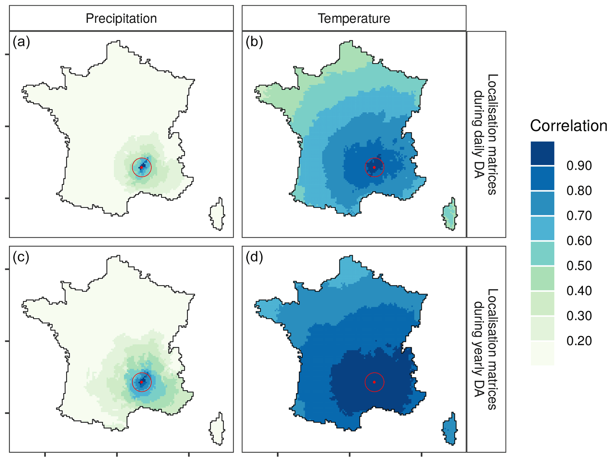
Figure 2Correlation matrices between values from the case study cell (in red) and all other cells, for daily (a, b) and yearly (c, d) data assimilation, for precipitation (a, c) and temperature (b, d).
3.5 Precipitation transformation
The Ensemble Kalman fitting scheme is optimal in a Gaussian framework, but daily and yearly precipitation follows a positive, skewed, and asymmetric distribution with a spike at zero for daily precipitation (Fig. 3). However, the nonnormality of daily precipitation is often neglected in data assimilation (e.g., Quintana-Segui et al., 2008; Bhargava and Danard, 1994; Soci et al., 2016), while Mahfouf et al. (2007) assume a lognormal distribution. Lien et al. (2013) and Devers et al. (2020a) applied an anamorphosis to precipitation, that consists in projecting the daily precipitation into a normal space where the analysis is carried out and mapping the analysis back into the original space using the inverse of the transformation (Wackernagel, 2003; Bertino et al., 2003). Devers et al. (2020a) showed that the impact of the Gaussian anamorphosis on daily precipitation is lower than the impact of localization, but that it improves estimates in areas with sparse observations. In the current study, two different strategies are selected to transform the precipitation depending on the DA timescale.
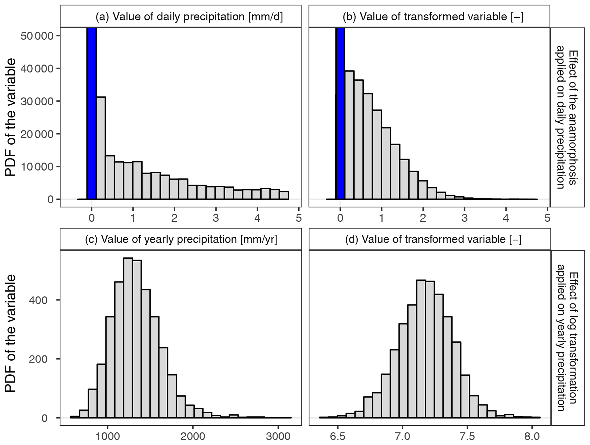
Figure 3Schematic view of the transformations applied to SCOPE Climate daily (a, b) and yearly (c, d) precipitation for the case study cell during the 1958–2008 period. The blue line represents zero values. For daily precipitation the x-axis of panels (a) and (b) is truncated at 5 mm d−1 for readability.
3.5.1 Daily DA
An anamorphosis transforming the raw daily precipitation X into a transformed variable Z is applied as follows:
with F(X) the cumulative density function X, G the cumulative density function of Z, and erf−1 the inverse error function satisfying .
The anamorphosis is defined locally for each grid cell with X the ensemble from SCOPE Climate during the 1958–2008 period, and the function is then piecewise-linearized (Simon and Bertino, 2009; Brankart et al., 2012). Outside of this period, the following rules are applied. Considering Xmin and Xmax the limit of the function domain, if then . If X>Xmax, then a linear regression fitted on values higher than the 99th percentile of nonzero precipitation is used, meaning that the tail of the transformed distribution is considered Gaussian (Devers et al., 2020a). However, even with the anamorphosis, the distribution obtained is closer to a truncated Gaussian pdf (probability density function) than a true Gaussian pdf (see Fig. 3a, b).
3.5.2 Yearly DA
For yearly precipitation, a simpler approach is implemented, assuming that yearly precipitation follows a lognormal distribution for each cell, thus making extrapolation more straightforward (Fig. 3). Yearly precipitation values X are thus transformed as follows, adding a 1 mm offset to allow for transforming zero total annual precipitation (even if this case is unlikely to happen in France):
3.5.3 Common processing
Irrespective of the timescale, the above transformation functions are applied before the analysis to (1) the background values, (2) the observations, and (3) the standard deviations. For the standard deviations, the nonlinearity of the transformations is taken into account as follows (see Lien et al., 2013):
with y the observation vector in the original space, σ the associated error, and the index trans indicating the variable transformed in the Gaussian space. After the analysis step, the analysis state Xa is then transformed back into the original space with the reciprocal functions of the anamorphosis and the logarithmic transformation.
3.6 Production of the reanalyses over 1871-2012
This section describes how the different reanalyses are produced over the 1871–2012 period (Fig. 4).
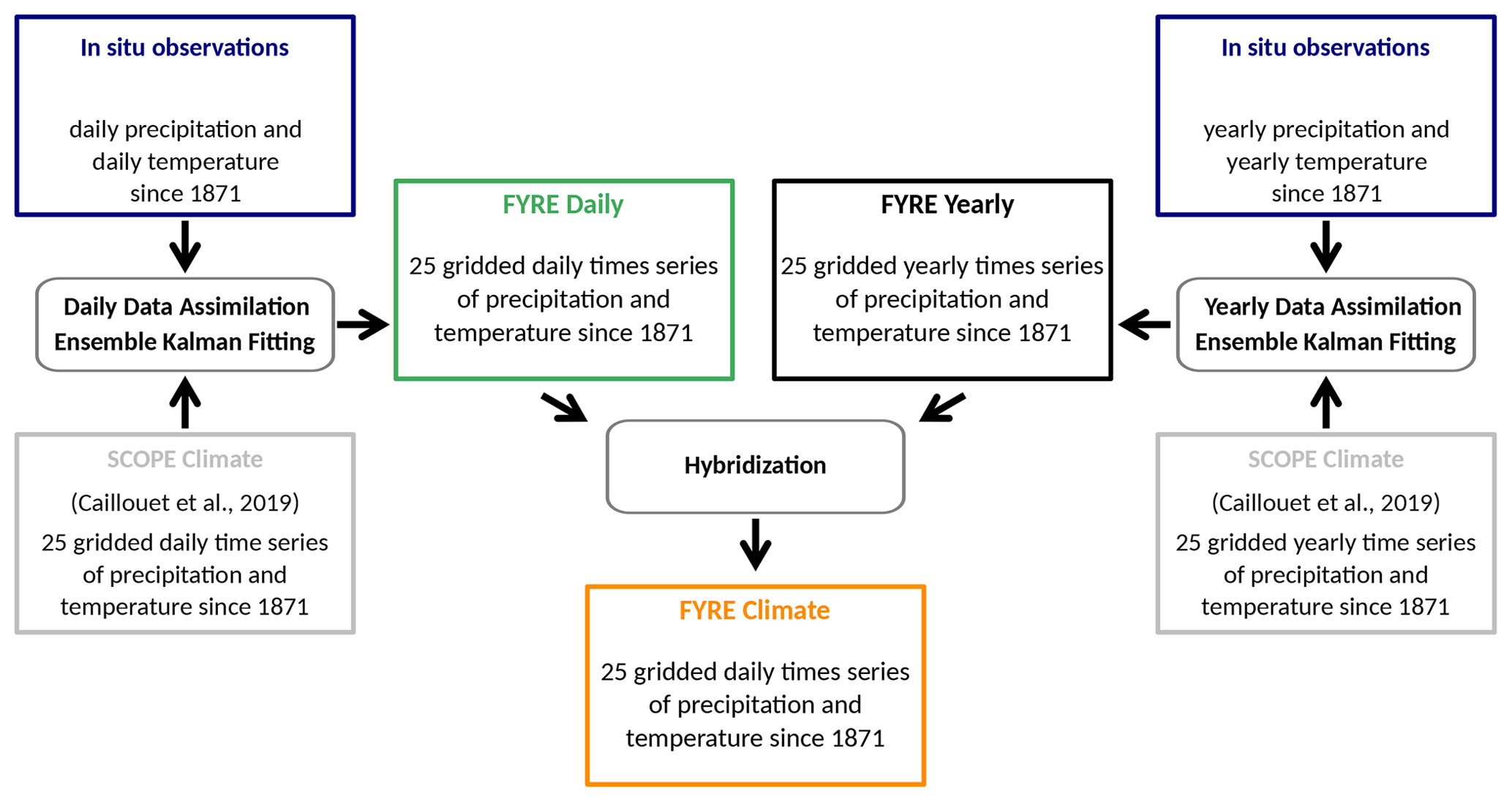
3.6.1 Application of the Ensemble Kalman fitting
The EnKf described in Sect. 3.1 is applied here for the two timescales. The FYRE Daily reanalysis is created using the scheme proposed by Devers et al. (2020a). The assimilation is done independently each day from 1 January 1871 to 29 December 2012 using the 25 SCOPE Climate members of temperature and precipitation as the background. The assimilated observations are daily in situ measurements of temperature and precipitation originating from the Météo-France database. FYRE Daily is thus a daily gridded reanalysis composed of 25 time series of precipitation and temperature fields.
The FYRE Yearly reanalysis is produced using yearly-averaged temperature values and yearly-accumulated precipitation. Once again the background is given by SCOPE Climate, and observations from the Météo-France database are assimilated (see Sect. 2.2). The assimilation is applied each year independently between 1871 and 2012, leading to the FYRE Yearly reanalysis composed of 25 yearly-averaged gridded time series of precipitation and temperature fields.
In FYRE Daily and FYRE Yearly, the assimilation is performed independently for temperature and precipitation, and independently at each time step. This means that assimilating precipitation has no impact on the temperature analysis (see the discussion in Devers et al., 2020a), and that assimilating an observation at a given time step has no effect on the analysis at another time step.
3.6.2 Hybridization
Finally, the FYRE Climate daily product combining the information of the daily and yearly reanalyses is derived through a hybridization between FYRE Daily and FYRE Yearly, following approaches adopted in numerous meteorological studies (Magand et al., 2018; Sheffield et al., 2006) and paleoclimate studies (Dirren and Hakim, 2005; Steiger and Hakim, 2016; Huntley and Hakim, 2010). The hybridization here aims at transforming daily values from FYRE Daily to match yearly values from FYRE Yearly.
For temperature, an additive transformation is commonly used and is adopted here (Dirren and Hakim, 2005; Steiger and Hakim, 2016; Huntley and Hakim, 2010). For precipitation, a multiplicative transformation is commonly used and is adopted here (Ngo-Duc et al., 2005; Keller et al., 2015). Note that such a transformation leads to largest changes in higher precipitation values, and that dry days from FYRE Daily will remain unchanged in FYRE Climate.
Each member of FYRE Climate is generated as follows. First, the ratio of precipitation β and temperature α are computed for each year based on the annual values of FYRE Yearly and FYRE Daily:
where y and d are the year and day considered, D the number of days during year y, c the cell, P and T the value of precipitation and temperature, respectively, with the index defining the dataset considered: daily for FYRE Daily and yearly for FYRE Yearly. Then, the time series of FYRE Climate are computed using the previously defined ratio and the daily time series of FYRE Daily:
with notations as above. The climate index refers to the final FYRE Climate values. This process leads to two daily 25-member ensemble products over the 1871–2012 period: FYRE Daily and FYRE Climate, whose differences are assessed below.
The first part of the results section is dedicated to the comparison between SCOPE Climate/FYRE Daily/FYRE Climate, and (1) the Safran reanalysis, (2) the monthly homogenized series (SMR) and (3) the European pattern climatology (EPC). A second part will provide examples of time series and extreme events to give a more precise idea of the characteristics of each dataset.
4.1 Comparison with the Safran reanalysis
An initial verification is done using the Safran reanalysis as a reference (Fig. 5). Scores are averaged over the 1960–2000 period and the ensemble median is displayed to provide a robust estimate of the central tendency of the ensemble. A more detailed year-by-year evaluation is proposed in the next section.
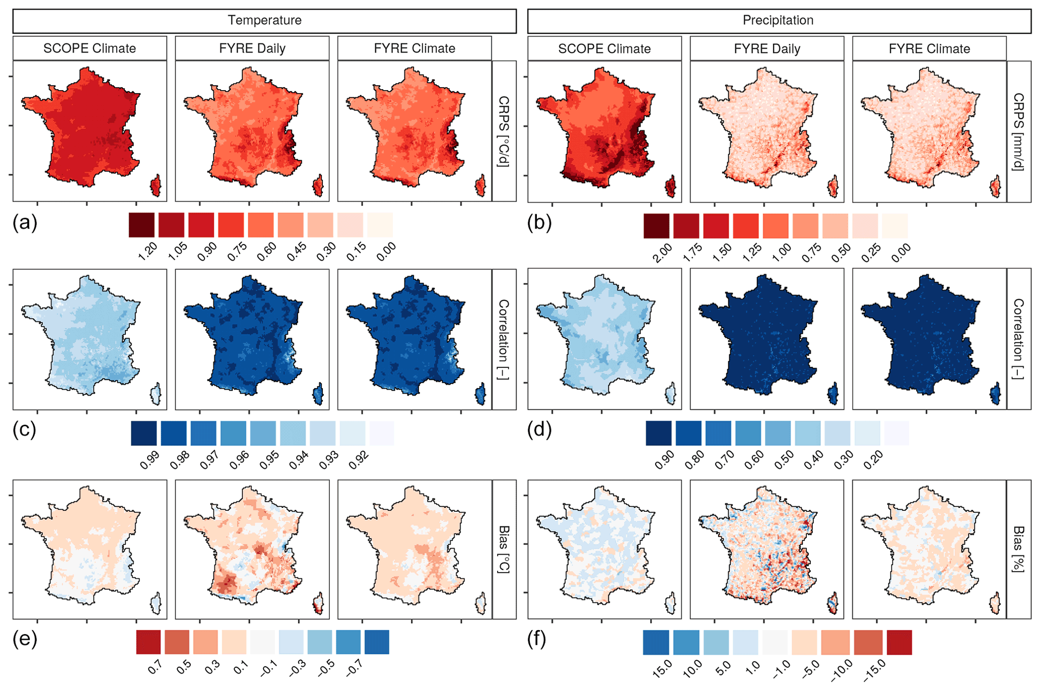
Figure 5Mean of daily continuous ranked probability score (CRPS) (a, b), daily correlation (c, d) and daily bias (e, f) between Safran and SCOPE Climate, FYRE Daily, and FYRE Climate for the 1960–2000 period for temperature (a, c, e) and precipitation (b, d, f). Correlation and bias are median values over each ensemble.
For temperature, over the 1960–2000 period, the behavior of FYRE Daily and FYRE Climate is similar to the Safran reanalysis with a low CRPS and a high daily correlation (see Fig. 5a, c, e). The impact of DA can be evaluated by comparing the background and reanalysis metrics. SCOPE Climate shows a higher CRPS and a lower daily correlation with Safran, but a slightly lower daily bias than the two reanalyses for specific areas. These differences may be explained by the assimilation of mean daily temperature that is computed using the minimum and maximum temperature, while the mean daily temperature in Safran is computed from hourly data. Indeed, this difference in the computation leads to a difference in the estimation of the mean daily temperature when the diurnal cycle is not perfectly symmetric. Biases shown by FYRE Daily are highly reduced in FYRE Climate, showing the benefits of the hybridization.
Panels b, d, f of Fig. 5 demonstrate the interest of DA concerning precipitation. The FYRE Daily and FYRE Climate reanalyses have a much lower CRPS and a much higher correlation with Safran than SCOPE Climate all over France. Although some differences are of the opposite sign on contiguous cells, there is a clear underestimation of FYRE Daily precipitation in mountainous areas, which is highly reduced in FYRE Climate, reaching values between −5 % and 5 %.
4.2 Comparison to the monthly homogenized series
In order to produce a verification constant over time – i.e with a rather steady number of validation stations – the analysis is divided into two periods. The reanalyses are compared to the monthly homogenized series (SMR) over the 1959–2009 period and the 1900–2000 period, that include 1583 and 332 stations respectively for precipitation and 308 and 88 for temperature (see Sect. 2.4.2). Scores (bias, correlation, and RMSE) are computed for each station and then averaged over France to provide a synthetic assessment of the performance with respect to SMR.
4.2.1 Over the 1959–2009 period
For temperature, the Safran reanalysis is negatively biased with respect to SMR (Fig. 6a, c, e). This difference is probably induced by differences in the computation of the mean daily temperature (see above), and the nonstationarity of the bias over time could reflect the asymmetric evolution of the minimum and maximum temperature. The bias of the background SCOPE Climate is around 0 at the start of the period and slowly degrades towards negative values, resulting from an underestimation of the recent warming already noted by Caillouet et al. (2019). FYRE Daily and FYRE Climate both display a much smaller negative bias – with values around −0.2 ∘C – and relatively constant over the last 30 years. SCOPE Climate has a lower correlation than all other products over the entire period. The FYRE Daily and FYRE Climate reanalyses show a higher correlation than Safran, and an uncertainty – defined by the spread of the ensemble – quite reduced compared to SCOPE Climate. A similar analysis may be drawn for the RMSE. FYRE Daily shows slightly lower RMSE values than FYRE Climate, but the two reanalyses perform overall similarly, and much better than SCOPE Climate or even Safran.
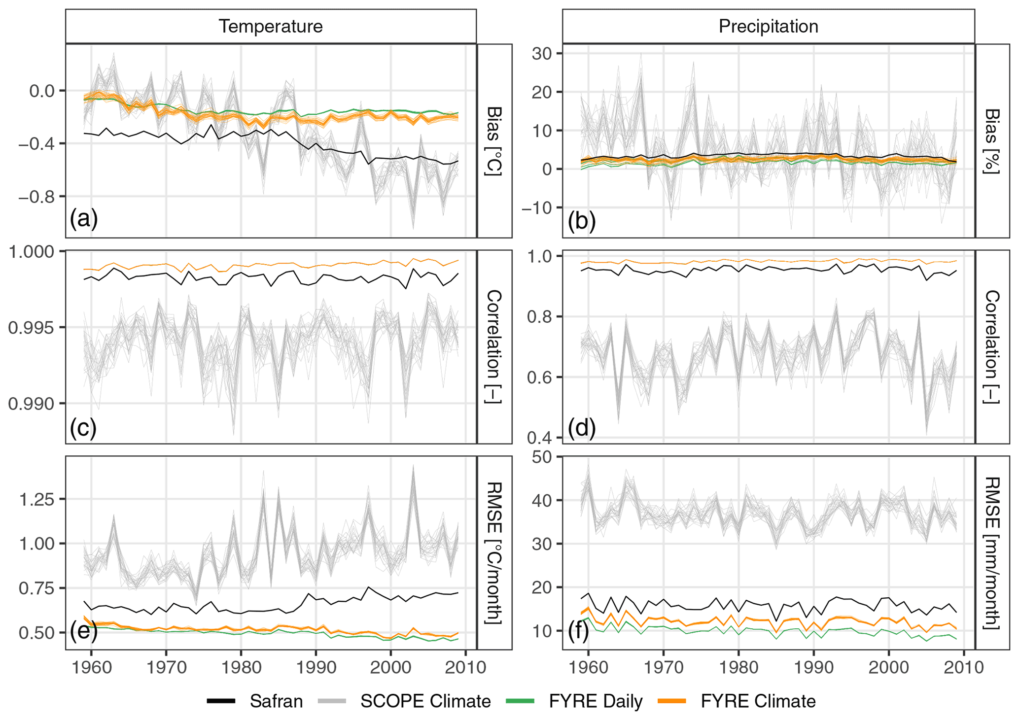
Figure 6Evolution of the mean monthly bias (a, b), correlation (c, d) and root mean square error (RMSE, e, f) between the monthly homogenized series and each member of SCOPE Climate/FYRE Daily/FYRE Climate/Safran for temperature (a, c, e) and precipitation (b, d, f) between 1959 and 2009. See text for details. Please note that the correlation curve of FYRE Daily is actually hidden by that of FYRE Climate.
For precipitation, SCOPE Climate shows a bias with a high interannual variability (Fig. 6b). All reanalyses including Safran show a very low and constant bias, with a very small spread for FYRE Daily and FYRE Climate. The impact of DA on correlation is also very clear, with a 0.3 increase on average for FYRE Daily and FYRE Climate compared to SCOPE Climate. Once again, the spread of the ensemble is reduced through the DA over the entire period. Finally, the Safran reanalysis has slightly lower correlations than the FYRE Daily and the FYRE Climate reanalyses. The RMSE is four times higher in SCOPE Climate than in the reanalyses. Among those, FYRE Daily shows the lowest errors, followed by FYRE Climate and then by Safran.
Figure 6 shows an overall large impact of the DA that allows FYRE Daily and FYRE Yearly to reach higher performances (lower bias, higher correlation, and lower RMSE) than Safran – the current reference reanalysis – over the 1959–2009 period compared to the monthly homogenized series. This result may be surprising but has already been pointed out by Devers et al. (2020a) in their validation setups. Even if the same observations are assimilated in both reanalyses, many differences may explain this result, notably the two following ones: (1) Safran is based on the strong hypothesis of climatically homogeneous zones (of 15 cells each on average, but with large variations across France with up to 50 cells for one zone, see Vidal et al., 2010b), where values only depend on altitude, and not on the specific 8 km cell, and (2) as a background, Safran uses vertical profiles from the ERA-40 global reanalysis and operational Météo-France analyses after 2002 (for temperature), and from climatological values (for precipitation) as mentioned in Sect. 2.4.1, so with a larger spatial information content compared to SCOPE Climate used by FYRE Daily and FYRE Climate as a background. FYRE Climate and FYRE Daily have therefore more assets to match the individual time series at local stations composing SMR.
4.2.2 Over the 1900–2000 period
Most of the comments made above with the most recent SMR dataset are also valid here for the post-1950s period, and a focus is thus made on centennial evolutions.
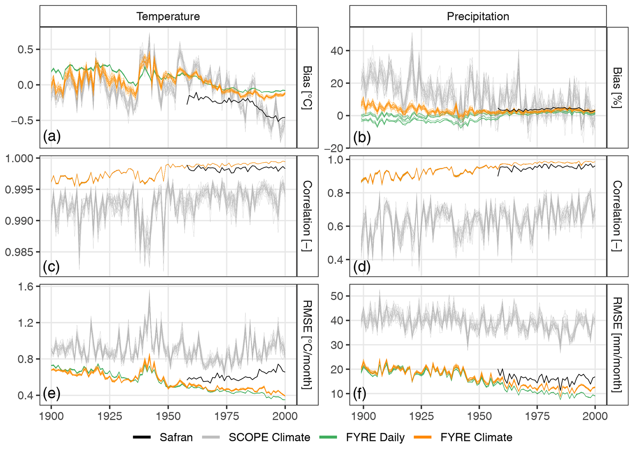
Figure 7Similar to Fig. 6, but over the 1900–2000 period with corresponding centennial homogenized time series.
The average bias of temperature between SMR and SCOPE Climate roughly varies between −0.5 and +0.5 ∘C (Fig. 7a). Before the 1950s, the two reanalyses do not share the same bias characteristics: FYRE Daily shows a slightly positive bias as well as a strong reduction of the ensemble spread after the 1900s, while FYRE Climate shows a strong dependency on the background and an ensemble spread that gradually shrinks over the 20th century. The correlation of the two reanalyses with SMR is clearly linked to the density of assimilated stations (see Fig. 1), with slightly reduced values before 1950, and drops during the two world wars. Nevertheless, values are consistently higher than those of the background. While RMSE for SCOPE Climate do not show any trend over the 20th century, those of the two reanalyses show a steady decrease from 0.7∘ per month in 1900 to 0.4∘ per month in 2000, only interrupted during the second world war as a consequence again of the drop in assimilated observations. During this period the background SCOPE Climate also shows a lower performance. This could be linked to the lack of surface observations assimilated across Western Europe in 20CR as a result of WWII, as shown by Cram et al. (2015) in their description of ISPDv2.
For precipitation, the background shows a global overestimation during the 1900–1960 period and an overall bias close to zero afterwards, but with a high interannual variability (+30 % to −10 %) (Fig. 7b). The absolute bias values are rather constant and much lower for the two reanalyses, albeit slightly increasing towards the beginning of the century. FYRE Daily (resp. FYRE Climate) shows a slightly negative (resp. positive) bias before 1960. FYRE Daily also shows an intriguing split of the ensemble before 1960, which will be discussed in Sect. 4.4 below. As for temperature, the correlation of the two reanalyses is quite a bit higher than those of the background, with slightly lower values during the first half of the century. The RMSE pattern is similar to that of temperature, with a steady decrease for the two reanalyses over the century, ranging from 20 mm per month in 1900 to around 10 mm per month in 2000, when SCOPE Climate values vary around 40 mm per month.
Overall, and beyond the evolution of ensemble-average values, the spread of the two reanalyses tends to shrink over the course of the century for all indicators, following the increasing number of assimilated observations.
4.3 Multidecadal variability
The long-term consistency between different datasets allows for further evaluation of the two reanalyses. To that end, anomalies are computed over the 1871–2012 period for several long-term datasets described in Sect. 2.4, using the 1900–2000 period as a reference. Anomalies are computed for each cell over France (see Sect. 2.4 for the number of cells in each dataset). Their median value is retained, smoothed with a 20-year rolling mean, and plotted in Fig. 8. Smoothed anomalies are computed for each member when available. EPC and SMR show a similar evolution of both temperature and precipitation over the 20th century. Negative temperature anomalies are found before the 1940s – from around −0.35∘ in 1910 and down to −0.6∘ in 1880 for EPC – and around the 1970s, and positive ones for other periods, with a steep recent warming from the 1980s onward reaching 0.5∘ in 1990 (Fig. 8a). Negative precipitation anomalies are found before 1910 and around the 1940s–1950s, and positive ones in other periods, including the most recent one.
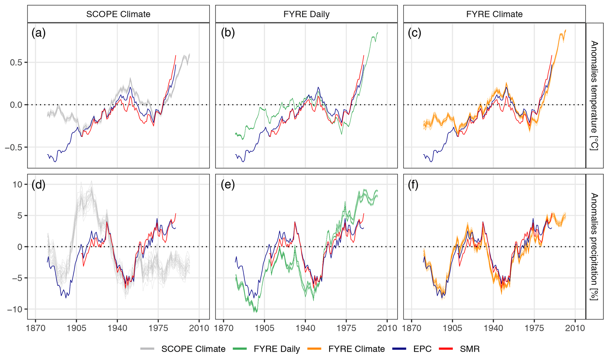
Figure 8Anomalies of annual temperature (a–c) and precipitation (d–f) averaged over France, and smoothed with a 20-year rolling mean. See text for details.
For temperature, SCOPE Climate anomalies are rather consistent with those from EPC and SMR over the 20th century. However, SCOPE Climate shows much higher – but still negative – anomalies than EPC before 1900, and underestimate the recent warming compared to EPC and SMR. FYRE Daily anomalies are closer to those of EPC and SMR after 1940 compared to SCOPE Climate – including during the recent warming –, but the original discrepancy at the beginning of the period extends to 1940. FYRE Climate anomalies are quite consistent with those of EPC and SMR from 1910 onward. However, before 1910, they are roughly constant around −0.2∘, i.e., much less negative than those of EPC. This discrepancy may come from the nonhomogeneity in underlying data in EPC: gridded observations after 1900 and climate field regression before that (see Sect. 2.4).
For precipitation, the high multidecadal variability of SCOPE Climate leads to positive anomalies over the 1890–1930 period, with values reaching nearly +10 %, when EPC and SMR values are only slightly positive. This is probably a bias inherited from the 20CR driving global extended reanalysis. Indeed, Bonnet et al. (2017) found much higher positive anomalies in 20CR precipitation over France than in the SMR over this period. SCOPE Climate also shows negative anomalies from 1960 onward when both EPC and SMR show positive anomalies. The overall multidecadal evolution of FYRE Daily is much more consistent with those of EPC and SMR, and the ensemble spread is quite reduced with respect to the background SCOPE Climate. However, anomalies are systematically shifted towards lower ones by 2 % to 3 % before 1950 and to higher ones – up to +5 % – after 1970, showing that only assimilating daily observations does not allow for accurate reproduction of multidecadal variability. Lastly, FYRE Climate is much more consistent with EPC and SMR long-term evolution, even with a small spread, as small as that of FYRE Daily.
4.4 Time series analysis
Time series over the Cévennes case study cell (see Fig. 1) derived from observations, Safran, SCOPE Climate, FYRE Daily, and FYRE Climate are presented in Figs. 9 and 10 to exemplify the behavior of the different datasets at different timescales and for selected periods differing in the amount of data assimilated: 1871–2012 at the annual timescale, years 1900, 1936, and 2000 at the monthly timescale, and June 1900, June 1936, and June 2000 at the daily timescale.
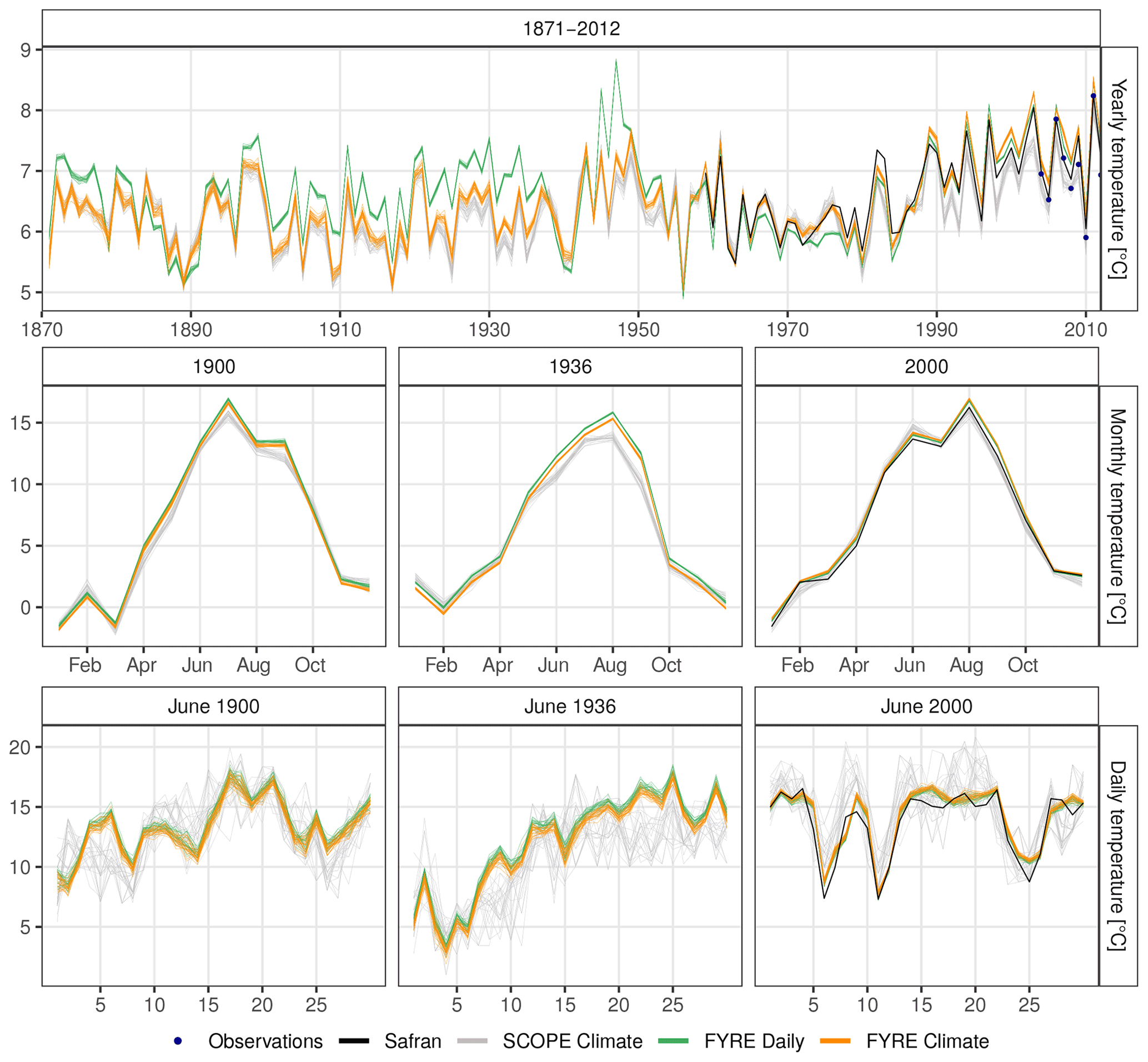
Figure 9Temperature time series of SCOPE Climate, FYRE Climate, FYRE Daily, and Safran over the case study cell for different periods and different time steps.

For temperature, all long-term datasets are well correlated at the annual timescale, but FYRE Daily values are systematically hotter before 1950. The ensemble spread is rather constant for SCOPE Climate while it is shrinking in the two reanalyses when more observations are assimilated. The underestimation of the recent warming by SCOPE Climate is once again visible here. The amplitude of the annual cycle for the three years considered appears underestimated in SCOPE Climate compared to the two reanalyses, an issue already identified by Caillouet et al. (2019) with respect to Safran. At the daily timescale, the ensemble spread is much reduced in both reanalyses compared to SCOPE Climate, even more so for June 2000 when many observations are assimilated close to – and not within – the case study cell considered.
For precipitation, Fig. 10 shows that DA tends to reduce the ensemble spread at the annual timescale even at the beginning of the period when only few data are assimilated. Large discrepancies are found for specific years between SCOPE Climate, FYRE Daily, and FYRE Climate. More specifically, extreme values are found for FYRE Daily in, e.g., 1879 and 1936, the latter year also showing a split of the ensemble, already noted earlier in Fig. 7. Similar comments may be drawn at the monthly and daily timescales, including the ensemble split over 1936, which is also present in FYRE Climate, but to a lesser extent. The puzzling behavior of FYRE Daily is in fact explained by two stations located close to the cell – less than 10 km, hence with high covariances – that give contradictory input to the DA scheme. Indeed, the two stations – #7235003, Sainte-Eulalie, 1350 m a.s.l., and #7326003, Usclades-et-Rieutord, 1270 m a.s.l. – both start providing precipitation data on 1 January 1936 and are assimilated, but with very different daily amounts (not shown here). At the end of 1936, the station #7235003 is closed, and FYRE Daily then shows a much more coherent ensemble as seen at the yearly timescale (Fig. 10, top panel). Hence, the large separation is due to the assimilation of two stations with contradictory values, possibly due to measurement errors. In an ideal framework where variables are Gaussian and observations are consistent, the analysis would lead to a Gaussian distribution. However, we deal here with daily precipitation whose distribution is (1) positive, (2) skewed, and (3) with a spike in zero. Note that we put an emphasis on this issue by applying a Gaussian anamorphosis prior to the assimilation, but this does not completely eliminate this issue. Moreover, and perhaps more importantly, measurement errors (coming, e.g., from exposure like proximity to walls or trees) may easily lead to inconsistent values within a given grid cell, and consequently to a multimodal analysis. It is interesting to note that the hybridization leads to a much reduced ensemble split, showing an unexpected advantage of FYRE Climate.
4.5 Examples of extreme events
The impact of DA on the representation of extreme events is investigated here with two events: (1) the cold month of December 1879 over the northeast of France (Fig. 11), and (2) an extreme precipitation event in the Cévennes area on 21 September 1890 (Fig. 12). To that end, three members – #8, #15 and #19 – have been randomly selected from SCOPE Climate, FYRE Daily, and FYRE Climate and are compared with the available observations at the time. The three randomly selected members are used to give an idea of the ensemble dispersion.
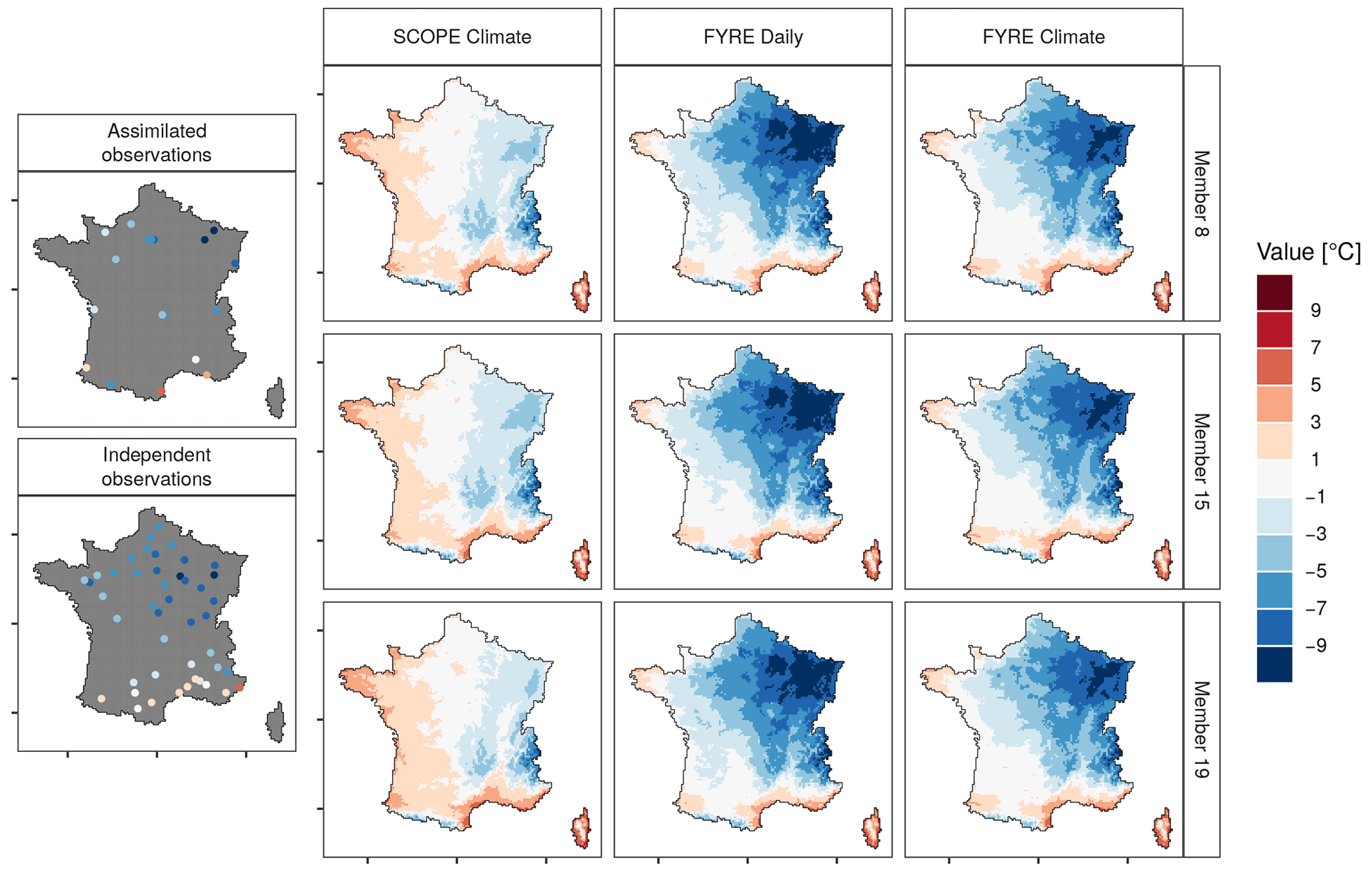
Figure 11Average daily mean temperature in France during December 1879 from observations (left panels), and from three randomly selected members of SCOPE Climate/FYRE Daily/FYRE Climate (right panels).
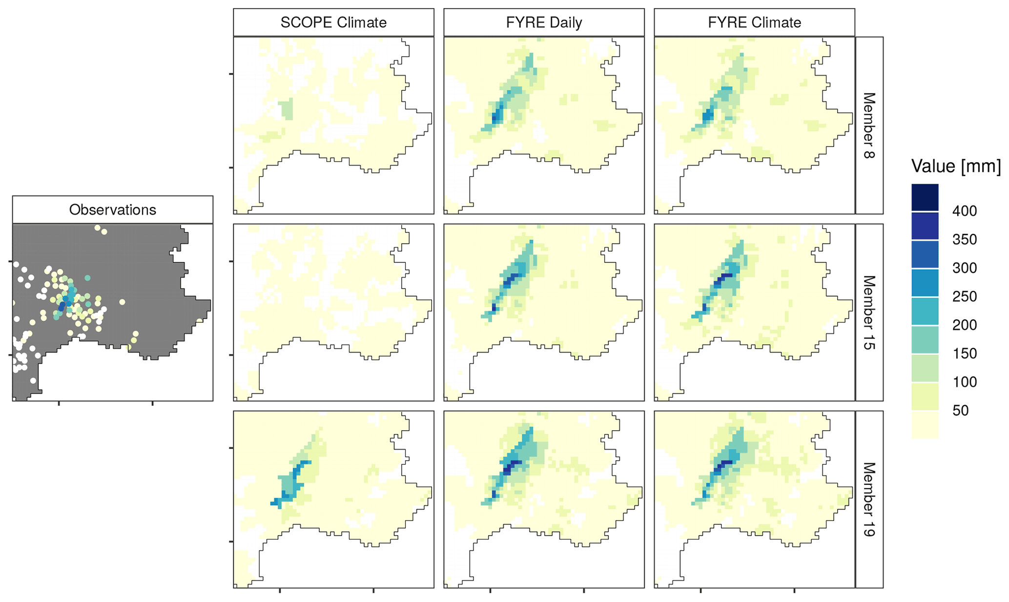
Figure 1221 September 1890 precipitation over southeast France from observations (left panel) and from three randomly selected members of SCOPE Climate/FYRE Daily/FYRE Climate (right panels).
4.5.1 An extreme cold wave
December 1879 is an extremely cold month in France as shown by the frost of the Loire, the Seine, the Saône, and the Rhône rivers (Dubrion, 2008) with a negative anomaly of −10.2 ∘C (Le Roy Ladurie et al., 2011, p. 202). The Annals of the Central Meteorological Office of France describe in detail the anticyclonic state lasting most of the month and the consequent very cold temperature over France and central Europe (Angot, 1881, pp. 19–23). Minimum values dropped for example below −25∘ in Paris on 10 December (Le Roy Ladurie and Séchet, 2009, pp. 43–44). The specificity of this cold wave is its duration, which led to December-averaged daily mean temperature reaching values well below −5 ∘C in the northeast of France, and even −10.3 ∘C for the Commercy station (id: 55122003). In order to obtain a more detailed validation of this event, monthly independent observations have been digitized from the Annals of the Central Meteorological Office of France (Mascart, 1881, pp. 217–240).
Figure 11 shows the December-averaged temperature over France, in the assimilated observations, in the independent observations, in the background SCOPE Climate, and in the two reanalyses. Compared to the observations, SCOPE Climate members largely overestimate the temperature everywhere except around the Mediterranean. This is especially true in the northeast, with more than 3 ∘C discrepancies. The impact of DA is quite clear, with both reanalyses showing much colder values, thanks to only 18 unevenly distributed assimilated stations. FYRE Climate is slightly less cold than FYRE Daily, but differences are minor overall. The independent observations confirm both the location and the intensity of the extreme cold temperature given by the two reanalyses, with, e.g., −9.4 ∘C in Troyes and −9.55 ∘C in Mirecourt located in the center of the event and a larger area with temperatures between −7 and −9 ∘C. The independent stations located in the south and west of France also allow us to grasp the positive impact of the DA outside the area impacted by the cold event.
4.5.2 An extreme precipitation event
At the end of September 1890, an extreme rainfall event in the Cévennes area (for an extended description of the event, see http://pluiesextremes.meteo.fr/france-metropole/Inondations-en-Cevennes-Crue-historique-de-l-Ardeche.html, last access: 1 September 2021) led to a record flood over the Ardèche river between 21 and 23 September 1890 (Sheffer et al., 2003; Naulet et al., 2005). Extreme precipitation amounts were recorded from 18 to 23 September reaching 971 mm at the Montpezat station (Météo-France, 1995, pp. 26–27). Figure 12 focuses on 21 September, when the highest daily amount of precipitation – 346 mm at Saint-André de Valeborgne, id: 30231001 – was recorded, with similar very high values in a small area oriented southwest to northeast (Fig. 12, left panel). Observations are mainly located in the central part of the Cévennes area, with few or no stations further north or south, thus impeding a global view of the event. The first two selected members of SCOPE Climate display very low precipitation values compared to observations, while the third one reaches values higher than 250 mm, but still underestimating recorded values. This latter member furthermore provides a spatial pattern of precipitation consistent with the classical shape of heavy precipitation events – called Cévenol events – in this region (see, e.g., Boudevillain et al., 2016). This high uncertainty in SCOPE Climate is dramatically reduced through DA, with both reanalyses providing precipitation values much closer to the observations, with amounts reaching 400 mm –, i.e., exceeding recorded ones – in some cells. A similar spatial pattern of the event is given by the two reanalyses, with a northeastern extension. Remaining differences between members reflect the uncertainty due the lack of observations, notably to the northeast, where reanalyses still suggest very high values. This example shows that DA thus allows us to strongly reduce uncertainty and to produce gridded meteorological fields more coherent with in situ observations.
5.1 Transforming precipitation
The anamorphosis chosen for transforming daily precipitation had already been applied with a large improvement of the analysis by Lien et al. (2013), and with a smaller one by Devers et al. (2020a). Implementing the anamorphosis, however, requires additional choices for extrapolating values, to both very low and positive values and to very high values (Lien et al., 2013, 2016). Choices are made here following Devers et al. (2020a).
A logarithmic transformation is applied here to yearly precipitation. The impact of this transformation has been studied in an experimental setup similar to the one proposed by Devers et al. (2020a) for daily precipitation, by varying the density of assimilated stations over the 1950–2000 period and evaluating the analysis on independent data. These experiments showed that the logarithmic transformation allows for canceling a dry bias in the analysis resulting from DA without transformation (not shown).
5.2 Estimating the observation error
Applying the DA scheme over the 1871–2012 period has put forward the need for quantifying the observation error, a key variable in the analysis step.
For the daily DA, the 1999–2012 period is rich in metadata, allowing for precisely defining the observation error based on the work of Météo-France and the World Meteorological Organization (WMO, 2014). Before 1999, the type of station is the only relevant metadata available. Devers et al. (2020a) translated the type of station into the framework of measurement errors linked to the maintained performance and site representativeness (Leroy, 2010; Leroy and Lèches, 2014) and found that making such an hypothesis improved both the reanalysis uncertainty and its reliability. This approach thus makes the most of available information, by distinguishing two classes of stations and associated measurement errors when no other metadata are available.
Estimating the observation error is even more difficult for the yearly DA, as no information is available at this timescale. Estimates used here may seem large (see Sect. 3.2), but a conservative choice has been made here to reflect, e.g., the homogeneity breaks that can be observed in the annual temperature and precipitation time series for some long-term stations. Further investigation of the yearly estimates of the observation error could focus on the intensity of the correction applied during the homogenization process of the SMR (Moisselin et al., 2002; Gibelin et al., 2014) at the yearly time step.
5.3 On the background uncertainty
The background for DA – SCOPE Climate – comes from a downscaling of the ensemble-mean fields of the 56-member Twentieth Century Reanalysis (Compo et al., 2011). SCOPE Climate may therefore underestimate the reconstruction uncertainty, especially at the end of the 19th century when few pressure observations were available, as discussed by Caillouet et al. (2016). Caillouet et al. (2019) showed that SCOPE Climate ensemble spread is presumably too small for temperature at the Paris-Montsouris station. However, DA experiments made here show that the background uncertainty is yet large enough to lead to very satisfactory results even before 1900 (see Sect. 4.5).
5.4 Assimilating yearly-averaged observations
Assimilating yearly observations allowed for the recovering of multidecadal variations consistent with other products such as SMR and EPC, as opposed to daily-only DA. For precipitation, this gain could be linked to the non-Gaussian properties of daily precipitation – even after anamorphosis – in contrast to log-transformed yearly precipitation. However, it is not so clear why this is the case with daily temperature. Nonetheless, Steiger and Hakim (2016) showed that assimilating low-frequency data improves the low-frequency components of reconstructions compared to using only high-frequency data.
In addition, most of the observations are assimilated twice in FYRE Climate: through the daily DA, and through the yearly DA. This can be problematic, as it is strongly advised not to assimilate the same observations twice in a DA scheme to avoid overemphasizing observations with respect to the background. However, in this case and similarly to recent paleoclimate DA studies (Steiger and Hakim, 2016, see, e.g.,) where the background is composed of the same dataset for the two timescales, the daily reanalysis is not used as a background for the yearly DA, thus maintaining relative independence.
5.5 On the hybridization
Choices made for the hybridization build on previous studies, notably for the additive formulation for temperature, in paleoclimate after DA of time-average observations (Steiger et al., 2014; Steiger and Hakim, 2016; Dirren and Hakim, 2005; Huntley and Hakim, 2010), but also for the more recent climate (Ngo-Duc et al., 2005; Weedon et al., 2011; Sheffield et al., 2004). A step further would be to make these additive corrections also depend on the season. To that end, the most direct approach would be to assimilate temperature observations at monthly or seasonal timescales.
The multiplicative correction applied to precipitation has been implemented following the work of Ngo-Duc et al. (2005) and Keller et al. (2015). The intensity of the correction is thus by construction higher during the wet season than during the dry season. Moreover, the correction has an impact only on wet days and does not affect the number of dry days. Methods have been developed to modify the number of wet days (Weedon et al., 2011; Sheffield et al., 2004) using wet-to-wet and dry-to-dry conditional probabilities of the compared dataset, but Sheffield et al. (2004) also note that they may compromise the spatial consistency.
5.6 On the validation
Validating a long-term product, and especially a reanalysis, is always difficult as (1) the amount of information available decreases when going back further in time, and (2) all available information is by definition used in the process. That is why a first study had been dedicated to the sole purpose of testing the DA scheme with a density of assimilated observations similar to selected years from the past, and therefore allowing for independent observations for validation (Devers et al., 2020a). More drastic validation setups like removing one-third of the observations over the 1971–2012 period would have resulted in no assimilated stations in the north of France or in the Alps, thus impeding any robust evaluation of the reanalysis over France. Additionally, it would be impossible to withhold the same set of stations for the whole period given the large changes in the observation network.
Hence, the choice was made to conduct the validation through comparison with a diversity of products. Even if these products are mainly based on similar observations, the comparison still allow for grasping the overall quality of the product assessed. Furthermore, the study of extreme events (Sect. 4.5) highlights the crucial value of the literary source when assessing a long-term product both in terms of quantitative or qualitative description. Further comparisons to other shorter products could be conducted, for example, with the E-OBS ensemble dataset available across Europe (Cornes et al., 2018). In order to better apprehend the characteristics of the reanalyses, an indirect validation using independent streamflow observations could also be performed through hydrological modeling as done in several studies (Raimonet et al., 2017; Caillouet et al., 2017; Smith et al., 2019).
The present study goal was to build on the work of Devers et al. (2020a) to provide a long-term daily reanalysis of precipitation and temperature at high resolution over France. Two reanalyses were produced based on DA using the SCOPE Climate downscaled reconstruction (Caillouet et al., 2019) as background. FYRE Daily (resp. FYRE Yearly) used daily (resp. annual) observations in the DA process. These two intermediate reanalyses were then hybridized to derived the final FYRE Climate reanalysis corresponding to the study objective.
Section 4.1 showed that both FYRE Daily and FYRE Climate have strong similarities with the current reference Safran reanalysis over the period 1950–2000, and clearly improve on the SCOPE Climate background. Devers et al. (2020a) even found that FYRE Daily performs better than Safran with respect to independent data on a set of experiments over the 2009–2012 period. Section 4.2 also showed better performance (bias, correlation, RMSE) than SCOPE Climate but also than Safran when compared to monthly homogenized time series. Section 4.5 lastly showed that both reanalyses perform very well in reproducing extreme temperature and precipitation events, which was a weak point in SCOPE Climate (Caillouet et al., 2019). All these elements clearly show the benefit of data assimilation for century-long reconstructions.
Section 4.3 highlighted the most important difference between FYRE Daily and FYRE Climate. While FYRE Daily clearly improves on the reconstruction of multidecadal variability as inferred from the SMR and EPC long-term datasets at the scale of France, FYRE Climate displays variations much more consistent with these datasets than FYRE Daily, for both precipitation and temperature, and for all subperiods. FYRE Climate thus provides the best features, by performing as well as FYRE Daily on small timescales, and much better at longer timescales.
FYRE Climate is therefore the final product of this work: a daily surface reanalysis of precipitation and temperature at the daily timescale and at a 8 km resolution over France between 1 January 1871 and 29 December 2012. Moreover, FYRE Climate is an ensemble reanalysis composed of 25 members whose spread reflects the uncertainty in both the reconstruction used as background for DA, and the assimilated observations. As such, it is the first century-long surface reanalysis at a country scale, paving the way for assessing the long-term evolution of climate at the local scale and studying past extreme meteorological events. To this aim, FYRE Climate is made available freely to the research community through two joined datasets: precipitation (Devers et al., 2020b) and temperature (Devers et al., 2020c).
FYRE Climate is available as netcdf files on the zenodo.org platform. For practical reasons, the dataset is split into one for precipitation (https://doi.org/10.5281/zenodo.4005573, Devers et al., 2020b) and another for temperature (https://doi.org/10.5281/zenodo.4006472, Devers et al., 2020c). Each dataset comprises 25 netcdf files, one for each ensemble member. Please note that ensemble member #1 for temperature should be associated with member #1 for precipitation, and so on. Values are available over the Safran grid (see Vidal et al., 2010a), but only for grid cells located within French borders, as for SCOPE Climate (Caillouet et al., 2019). SCOPE Climate, described in Caillouet et al. (2019), is available as netcdf files on the Zenodo platform for precipitation (https://doi.org/10.5281/zenodo.1299760, Caillouet et al., 2018a), temperature (https://doi.org/10.5281/zenodo.1299712, Caillouet et al., 2018b), and reference evapotranspiration (https://doi.org/10.5281/zenodo.1251843, Caillouet et al., 2018c).
AD designed the study and the analysis with support of JPV, CL, and OV. AD performed the analysis and drafted the manuscript. All authors revised the manuscript.
The authors declare that they have no conflict of interest.
Publisher’s note: Copernicus Publications remains neutral with regard to jurisdictional claims in published maps and institutional affiliations.
The authors would like to thank Météo-France for providing access to the Safran surface reanalysis, the monthly homogenized series, as well as to surface observations and associated metadata. Analyses were performed in R (R Core Team, 2018) with packages ncdf4 (Pierce, 2015), dplyr (Wickham et al., 2017), tidyr (Wickham and Henry, 2018), ggplot2 (Wickham, 2009), fst (Klik, 2018) and sp (Bivand et al., 2013).
Alexandre Devers' PhD thesis was funded by Irstea (now INRAE) and CNR.
This paper was edited by Hans Linderholm and reviewed by two anonymous referees.
Anderson, J. L.: Localization and Sampling Error Correction in Ensemble Kalman Filter Data Assimilation, Mon. Weather Rev., 140, 2359–2371, https://doi.org/10.1175/MWR-D-11-00013.1, 2012. a
Angot, A.: Annales du Bureau Central Météorologique de France – Année 1879. Tome II. Bulletin des observations françaises et revue climatologique. Revue climatologique mensuelle pour la France et les contrées voisines, Gauthiers-Villars, Paris, France, 1881. a
Annan, J. D. and Hargreaves, J. C.: Identification of climatic state with limited proxy data, Clim. Past, 8, 1141–1151, https://doi.org/10.5194/cp-8-1141-2012, 2012. a
Asch, M., Bocquet, M., and Nodet, M.: Data assimilation: methods, algorithms, and applications, in: Fundamentals of Algorithms, Society for Industrial and Applied Mathematics (SIAM), Philadelphia, PA, USA, available at: https://hal.inria.fr/hal-01402885 (last access: 1 September 2021), 2016. a
Ben Daoud, A., Sauquet, E., Bontron, G., Obled, C., and Lang, M.: Daily quantitative precipitation forecasts based on the analogue method: Improvements and application to a French large river basin, Atmos. Res., 169, 147–159, https://doi.org/10.1016/j.atmosres.2015.09.015, 2016. a
Bertino, L., Evensen, G., and Wackernagel, H.: Sequential Data Assimilation Techniques in Oceanography, Int. Stat. Rev., 71, 223–241, https://doi.org/10.1111/j.1751-5823.2003.tb00194.x, 2003. a
Bhargava, M. and Danard, M.: Application of Optimum Interpolation to the Analysis of Precipitation in Complex Terrain, J. Appl. Meteorol., 33, 508–518, https://doi.org/10.1175/1520-0450(1994)033<0508:AOOITT>2.0.CO;2, 1994. a
Bhend, J., Franke, J., Folini, D., Wild, M., and Brönnimann, S.: An ensemble-based approach to climate reconstructions, Clim. Past, 8, 963–976, https://doi.org/10.5194/cp-8-963-2012, 2012. a, b, c
Bivand, R. S., Pebesma, E., and Gomez-Rubio, V.: Applied spatial data analysis with R, Second edition, Springer, NY, USA, 2013. a
Boé, J. and Habets, F.: Multi-decadal river flow variations in France, Hydrol. Earth Syst. Sci., 18, 691–708, https://doi.org/10.5194/hess-18-691-2014, 2014. a
Bonnet, R., Boé, J., Dayon, G., and Martin, E.: Twentieth-Century Hydrometeorological Reconstructions to Study the Multidecadal Variations of the Water Cycle Over France, Water Resour. Res., 53, 8366–8382, https://doi.org/10.1002/2017WR020596, 2017. a, b
Bonnet, R., Boé, J., and Habets, F.: Influence of multidecadal variability on high and low flows: the case of the Seine basin, Hydrol. Earth Syst. Sci., 24, 1611–1631, https://doi.org/10.5194/hess-24-1611-2020, 2020. a
Boudevillain, B., Delrieu, G., Wijbrans, A., and Confoland, A.: A high-resolution rainfall re-analysis based on radar–raingauge merging in the Cévennes-Vivarais region, France, J. Hydrol., 541, 14–23, https://doi.org/10.1016/j.jhydrol.2016.03.058, 2016. a
Brankart, J.-M., Testut, C.-E., Béal, D., Doron, M., Fontana, C., Meinvielle, M., Brasseur, P., and Verron, J.: Towards an improved description of ocean uncertainties: effect of local anamorphic transformations on spatial correlations, Ocean Sci., 8, 121–142, https://doi.org/10.5194/os-8-121-2012, 2012. a
Brigode, P., Brissette, F., Nicault, A., Perreault, L., Kuentz, A., Mathevet, T., and Gailhard, J.: Streamflow variability over the 1881–2011 period in northern Québec: comparison of hydrological reconstructions based on tree rings and geopotential height field reanalysis, Clim. Past, 12, 1785–1804, https://doi.org/10.5194/cp-12-1785-2016, 2016. a
Brown, T. A.: Admissible Scoring Systems for Continuous Distributions., Tech. rep., Rand Corp., Santa Monica, CA, USA, available at: https://eric.ed.gov/?id=ED135799 (last access: 6 September 2021), 1974. a
Burgers, G., van Leeuwen, P. J., and Evensen, G.: Analysis Scheme in the Ensemble Kalman Filter, Mon. Weather Rev., 126, 1719–1724, https://doi.org/10.1175/1520-0493(1998)126<1719:asitek>2.0.co;2, 1998. a
Caillouet, L., Vidal, J.-P., Sauquet, E., and Graff, B.: Probabilistic precipitation and temperature downscaling of the Twentieth Century Reanalysis over France, Clim. Past, 12, 635–662, https://doi.org/10.5194/cp-12-635-2016, 2016. a, b, c
Caillouet, L., Vidal, J.-P., Sauquet, E., Devers, A., and Graff, B.: Ensemble reconstruction of spatio-temporal extreme low-flow events in France since 1871, Hydrol. Earth Syst. Sci., 21, 2923–2951, https://doi.org/10.5194/hess-21-2923-2017, 2017. a, b, c
Caillouet, L., Vidal, J.-P., Sauquet, E., Graff, B., and Soubeyroux, J.-M.: SCOPE Climate: precipitation, Zenodo [data set], https://doi.org/10.5281/zenodo.1299760, 2018a. a, b
Caillouet, L., Vidal, J.-P., Sauquet, E., Graff, B., and Soubeyroux, J.-M.: SCOPE Climate: temperature, Zenodo [data set], https://doi.org/10.5281/zenodo.1299712, 2018b. a, b
Caillouet, L., Vidal, J.-P., Sauquet, E., Graff, B., and Soubeyroux, J.-M.: SCOPE Climate: Penman-Monteith reference evapotranspiration, Zenodo [data set], https://doi.org/10.5281/zenodo.1251843, 2018c. a, b
Caillouet, L., Vidal, J.-P., Sauquet, E., Graff, B., and Soubeyroux, J.-M.: SCOPE Climate: a 142-year daily high-resolution ensemble meteorological reconstruction dataset over France, Earth Syst. Sci. Data, 11, 241–260, https://doi.org/10.5194/essd-11-241-2019, 2019. a, b, c, d, e, f, g, h, i, j, k, l, m
Capel, C.: Qui sont les observateurs bénévoles de Météo France?, Ethnologie française, 39, 631–637, https://doi.org/10.3917/ethn.094.0631, 2009. a
Carrassi, A., Bocquet, M., Bertino, L., and Evensen, G.: Data assimilation in the geosciences: An overview of methods, issues, and perspectives, WIRES Clim. Change, 9, e535, https://doi.org/10.1002/wcc.535, 2018. a
Casty, C., Handorf, D., and Sempf, M.: Combined winter climate regimes over the North Atlantic European sector 1766–2000, Geophys. Res. Lett., 32, L13801, https://doi.org/10.1029/2005GL022431, 2005. a
Casty, C., Raible, C. C., Stocker, T. F., Wanner, H., and Luterbacher, J.: A European pattern climatology 1766–2000, Clim. Dynam., 29, 791–805, https://doi.org/10.1007/s00382-007-0257-6, 2007. a
Clark, M., Gangopadhyay, S., Hay, L., Rajagopalan, B., and Wilby, R.: The Schaake Shuffle: A Method for Reconstructing Space–Time Variability in Forecasted Precipitation and Temperature Fields, J. Hydrometeorol., 5, 243–262, https://doi.org/10.1175/1525-7541(2004)005<0243:tssamf>2.0.co;2, 2004. a
Compo, G. P., Whitaker, J. S., Sardeshmukh, P. D., Matsui, N., Allan, R. J., Yin, X., Gleason, B. E., Vose, R. S., Rutledge, G., Bessemoulin, P., Brönnimann, S., Brunet, M., Crouthamel, R. I., Grant, A. N., Groisman, P. Y., Jones, P. D., Kruk, M. C., Kruger, A. C., Marshall, G. J., Maugeri, M., Mok, H. Y., Nordli, Ø., Ross, T. F., Trigo, R. M., Wang, X. L., Woodruff, S. D., and Worley, S. J.: The Twentieth Century Reanalysis Project, Q. J. Roy. Meteor. Soc., 137, 1–28, https://doi.org/10.1002/qj.776, 2011. a, b
Cornes, R. C., van der Schrier, G., van den Besselaar, E. J. M., and Jones, P. D.: An Ensemble Version of the E-OBS Temperature and Precipitation Data Sets, J. Geophys. Res.-Atmos., 123, 9391–9409, https://doi.org/10.1029/2017JD028200, 2018. a
Cram, T. A., Compo, G. P., Yin, X., Allan, R. J., McColl, C., Vose, R. S., Whitaker, J. S., Matsui, N., Ashcroft, L., Auchmann, R., Bessemoulin, P., Brandsma, T., Brohan, P., Brunet, M., Comeaux, J., Crouthamel, R., Gleason Jr, B. E., Groisman, P. Y., Hersbach, H., Jones, P. D., Jónsson, T., Jourdain, S., Kelly, G., Knapp, K. R., Kruger, A., Kubota, H., Lentini, G., Lorrey, A., Lott, N., Lubker, S. J., Luterbacher, J., Marshall, G. J., Maugeri, M., Mock, C. J., Mok, H. Y., Nordli, Ø., Rodwell, M. J., Ross, T. F., Schuster, D., Srnec, L., Valente, M. A., Vizi, Z., Wang, X. L., Westcott, N., Woollen, J. S., and Worley, S. J.: The International Surface Pressure Databank version 2, Geosci. Data J., 2, 31–46, https://doi.org/10.1002/gdj3.25, 2015. a
Dayon, G., Boé, J., and Martin, E.: Transferability in the future climate of a statistical downscaling method for precipitation in France, J. Geophys. Res.-Atmos., 120, 1023–1043, https://doi.org/10.1002/2014JD022236, 2015. a
Devers, A., Vidal, J.-P., Lauvernet, C., Graff, B., and Vannier, O.: A framework for high-resolution meteorological surface reanalysis through offline data assimilation in an ensemble of downscaled reconstructions, Q. J. Roy. Meteor. Soc., 146, 153–173, https://doi.org/10.1002/qj.3663, 2020a. a, b, c, d, e, f, g, h, i, j, k, l, m, n, o, p, q, r, s, t, u
Devers, A., Vidal, J.-P., Lauvernet, C., and Vannier, O.: FYRE Climate: Precipitation, Zenodo [data set], https://doi.org/10.5281/zenodo.4005573, 2020b. a, b, c
Devers, A., Vidal, J.-P., Lauvernet, C., and Vannier, O.: FYRE Climate: Temperature, Zenodo [data set], https://doi.org/10.5281/zenodo.4006472, 2020c. a, b, c
Dirren, S. and Hakim, G. J.: Toward the assimilation of time-averaged observations, Geophys. Res. Lett., 32, L04804, https://doi.org/10.1029/2004GL021444, 2005. a, b, c, d
Dubrion, R.: Le climat et ses excés, Féret, Bordeaux, France, 2008. a
Evensen, G.: The Ensemble Kalman Filter: theoretical formulation and practical implementation, Ocean Dynam., 53, 343–367, https://doi.org/10.1007/s10236-003-0036-9, 2003. a, b
Franke, J., Brönnimann, S., Bhend, J., and Brugnara, Y.: A monthly global paleo-reanalysis of the atmosphere from 1600 to 2005 for studying past climatic variations, Scientific Data, 4, 170076, https://doi.org/10.1038/sdata.2017.76, 2017. a
Galliot, M.: Le réseau des observateurs bénévoles en France, La Météorologie, 40, 64–67, https://doi.org/10.4267/2042/36266, 2003. a
Gandin, L. V.: Objective analysis of meteorological fields, Israel Program for Scientific Translations, Jerusalem, Isreal, https://doi.org/10.1002/qj.49709239320, 1965. a
Gibelin, A.-L., Dubuisson, B., Corre, L., Jourdain, S., Laval, L., Piquemal, J.-M., Mestre, O., Dennetière, D., Desmidt, S., and Tamburini, A.: Evolution de la température en France depuis les années 1950: Constitution d'un nouveau jeu de séries homogénéisées de référence, La Météorologie, 87, 45–53, https://doi.org/10.4267/2042/54336, 2014. a, b, c, d
Goosse, H., Renssen, H., Timmermann, A., Bradley, R. S., and Mann, M. E.: Using paleoclimate proxy-data to select optimal realisations in an ensemble of simulations of the climate of the past millennium, Clim. Dynam., 27, 165–184, https://doi.org/10.1007/s00382-006-0128-6, 2006. a
Hakim, G. J., Emile-Geay, J., Steig, E. J., Noone, D., Anderson, D. M., Tardif, R., Steiger, N., and Perkins, W. A.: The last millennium climate reanalysis project: Framework and first results, J. Geophys. Res.-Atmos., 121, 6745–6764, https://doi.org/10.1002/2016jd024751, 2016. a
Horton, P. and Brönnimann, S.: Impact of global atmospheric reanalyses on statistical precipitation downscaling, Clim. Dynam., 52, 5189–5211, https://doi.org/10.1007/s00382-018-4442-6, 2018. a
Houtekamer, P. L. and Mitchell, H. L.: Data Assimilation Using an Ensemble Kalman Filter Technique, Mon. Weather Rev., 126, 796–811, https://doi.org/10.1175/1520-0493(1998)126<0796:dauaek>2.0.co;2, 1998. a, b
Houtekamer, P. L. and Zhang, F.: Review of the Ensemble Kalman Filter for Atmospheric Data Assimilation, Mon. Weather Rev., 144, 4490–4525, https://doi.org/10.1175/MWR-D-15-0440.1, 2016. a
Huntley, H. S. and Hakim, G. J.: Assimilation of time-averaged observations in a quasi-geostrophic atmospheric jet model, Clim. Dynam., 35, 995–1009, https://doi.org/10.1007/s00382-009-0714-5, 2010. a, b, c, d
Keller, V. D. J., Tanguy, M., Prosdocimi, I., Terry, J. A., Hitt, O., Cole, S. J., Fry, M., Morris, D. G., and Dixon, H.: CEH-GEAR: 1 km resolution daily and monthly areal rainfall estimates for the UK for hydrological and other applications, Earth Syst. Sci. Data, 7, 143–155, https://doi.org/10.5194/essd-7-143-2015, 2015. a, b, c
Klik, M.: fst: Lightning Fast Serialization of Data Frames for R, R package version 0.8.4, available at: https://cran.r-project.org/package=fst (last access: 8 September 2021), 2018. a
Kuentz, A., Mathevet, T., Gailhard, J., and Hingray, B.: Building long-term and high spatio-temporal resolution precipitation and air temperature reanalyses by mixing local observations and global atmospheric reanalyses: the ANATEM model, Hydrol. Earth Syst. Sci., 19, 2717–2736, https://doi.org/10.5194/hess-19-2717-2015, 2015. a
Landelius, T., Dahlgren, P., Gollvik, S., Jansson, A., and Olsson, E.: A high-resolution regional reanalysis for Europe. Part 2: 2D analysis of surface temperature, precipitation and wind, Q. J. Roy. Meteor. Soc., 142, 2132–2142, https://doi.org/10.1002/qj.2813, 2016. a
Leroy, M.: Classification de performance maintenue, Technical note, Météo France: Direction des Systèmes d'Observation, Toulouse, France, 2010. a, b, c
Leroy, M. and Lèches, G.: Classification d'un site, Note technique, Météo France: Direction des Systèmes d'Observation, Toulouse, France, 2014. a, b, c
Le Roy Ladurie, E. and Séchet, G.: Histoire humaine et comparée du climat, vol. III, Fayard, Paris, France, 2009. a
Le Roy Ladurie, E., Rousseau, D., and Vazak, A.: Les fluctuations du climat de l'an mil à aujourd'hui, Fayard, Paris, France, 2011. a
Lien, G.-Y., Kalnay, E., and Miyoshi, T.: Effective assimilation of global precipitation: simulation experiments, Tellus A, 65, 19915, https://doi.org/10.3402/tellusa.v65i0.19915, 2013. a, b, c, d
Lien, G.-Y., Kalnay, E., Miyoshi, T., and Huffman, G. J.: Statistical Properties of Global Precipitation in the NCEP GFS Model and TMPA Observations for Data Assimilation, Mon. Weather Rev., 144, 663–679, https://doi.org/10.1175/MWR-D-15-0150.1, 2016. a
Lorenz, E. N.: Atmospheric Predictability as Revealed by Naturally Occurring Analogues, J. Atmos. Sci., 26, 636–646, https://doi.org/10.1175/1520-0469(1969)26<636:aparbn>2.0.co;2, 1969. a
Magand, C., Ducharne, A., Tilmant, François Le Moine, N., Sauquet, E., Mathevet, T., Vidal, J.-P., and Perrin, C.: Hybridation de réanalyses météorologiques de surface pour les zones de montagne : exemple du produit DuO sur le bassin de la Durance, La Houille Blanche, 104, 77–85, https://doi.org/10.1051/lhb/2018035, 2018. a
Mahfouf, J.-F., Brasnett, B., and Gagnon, S.: A Canadian precipitation analysis (CaPA) project: Description and preliminary results, Atmos.-Ocean, 45, 1–17, https://doi.org/10.3137/ao.v450101, 2007. a
Mascart, E., ed.: Annales du Bureau Central Météorologique de France – Année 1879. Tome II. Bulletin des observations françaises et revue climatologique. Première partie: Bulletin des observations francçaises, Gauthiers-Villars, Paris, France, 1881. a
Matsikaris, A., Widmann, M., and Jungclaus, J.: On-line and off-line data assimilation in palaeoclimatology: a case study, Clim. Past, 11, 81–93, https://doi.org/10.5194/cp-11-81-2015, 2015. a
Météo-France: Inventaire des épisodes de fortes pluies en Ardèche – Tome I: 1807–1927, Aubenas, France, 1995. a
Minvielle, M., Pagé, C., Céron, J.-P., and Besson, F.: Extension of the SIM Reanalysis by Combination of Observations and Statistical Downscaling, in: Engineering Geology for Society and Territory – Volume 1, edited by: Lollino, G., Manconi, A., Clague, J., Shan, W., and Chiarle, M., 189–192, Springer International Publishing, Cham, Switzerland, https://doi.org/10.1007/978-3-319-09300-0_36, 2015. a, b, c
Mitchell, T. D. and Jones, P. D.: An improved method of constructing a database of monthly climate observations and associated high-resolution grids, Int. J. Climatol., 25, 693–712, https://doi.org/10.1002/joc.1181, 2005. a
Moisselin, J.-M., Schneider, M., and Canellas, C.: Les changements climatiques en France au XXè siècle. Etude des longues séries homogénéisées de données de température et de précipitations, La Météorologie, 38, 45–56, https://doi.org/10.4267/2042/36233, 2002. a, b, c, d, e
Naulet, R., Lang, M., Ouarda, T. B. M. J., Coeur, D., Bobée, B., Recking, A., and Moussay, D.: Flood frequency analysis on the Ardèche river using French documentary sources from the last two centuries, J. Hydrol., 313, 58–78, https://doi.org/10.1016/j.jhydrol.2005.02.011, 2005. a
Ngo-Duc, T., Polcher, J., and Laval, K.: A 53-year forcing data set for land surface models, J. Geophys. Res.-Atmos., 110, D06116, https://doi.org/10.1029/2004JD005434, 2005. a, b, c
Pfister, L., Brönnimann, S., Schwander, M., Isotta, F. A., Horton, P., and Rohr, C.: Statistical reconstruction of daily precipitation and temperature fields in Switzerland back to 1864, Clim. Past, 16, 663–678, https://doi.org/10.5194/cp-16-663-2020, 2020. a
Pierce, D.: ncdf4: Interface to Unidata netCDF (Version 4 or Earlier) Format Data Files, R package version 1.15, available at: https://CRAN.R-project.org/package=ncdf4 (last access: 8 September 2021), 2015. a
Quintana-Segui, P., Moigne, P. L., Durand, Y., Martin, E., Habets, F., Baillon, M., Canellas, C., Franchisteguy, L., and Morel, S.: Analysis of Near-Surface Atmospheric Variables: Validation of the SAFRAN Analysis over France, J. Appl. Meteorol. Clim., 47, 92–107, https://doi.org/10.1175/2007jamc1636.1, 2008. a, b
Quintana-Seguí, P., Turco, M., Herrera, S., and Miguez-Macho, G.: Validation of a new SAFRAN-based gridded precipitation product for Spain and comparisons to Spain02 and ERA-Interim, Hydrol. Earth Syst. Sci., 21, 2187–2201, https://doi.org/10.5194/hess-21-2187-2017, 2017. a
Radanovics, S., Vidal, J.-P., Sauquet, E., Ben Daoud, A., and Bontron, G.: Optimising predictor domains for spatially coherent precipitation downscaling, Hydrol. Earth Syst. Sci., 17, 4189–4208, https://doi.org/10.5194/hess-17-4189-2013, 2013. a
Raimonet, M., Oudin, L., Thieu, V., Silvestre, M., Vautard, R., Rabouille, C., and Le Moigne, P.: Evaluation of Gridded Meteorological Datasets for Hydrological Modeling, J. Hydrometeorol., 18, 3027–3041, https://doi.org/10.1175/JHM-D-17-0018.1, 2017. a
R Core Team: R: A Language and Environment for Statistical Computing, R Foundation for Statistical Computing, Vienna, Austria, 2018. a
Sheffer, N. A., Enzel, Y., Benito, G., Grodek, T., Poart, N., Lang, M., Naulet, R., and Cœur, D.: Paleofloods and historical floods of the Ardèche River, France, Water Resour. Res., 39, 1376, https://doi.org/10.1029/2003WR002468, 2003. a
Sheffield, J., Ziegler, A. D., Wood, E. F., and Chen, Y.: Correction of the High-Latitude Rain Day Anomaly in the NCEP–NCAR Reanalysis for Land Surface Hydrological Modeling, J. Climate, 17, 3814–3828, https://doi.org/10.1175/1520-0442(2004)017<3814:COTHRD>2.0.CO;2, 2004. a, b, c
Sheffield, J., Goteti, G., and Wood, E. F.: Development of a 50-Year High-Resolution Global Dataset of Meteorological Forcings for Land Surface Modeling, J. Climate, 19, 3088–3111, https://doi.org/10.1175/JCLI3790.1, 2006. a
Simon, E. and Bertino, L.: Application of the Gaussian anamorphosis to assimilation in a 3-D coupled physical-ecosystem model of the North Atlantic with the EnKF: a twin experiment, Ocean Sci., 5, 495–510, https://doi.org/10.5194/os-5-495-2009, 2009. a
Slonosky, V. C.: Wet winters, dry summers? Three centuries of precipitation data from Paris, Geophys. Res. Lett., 29, 34-1–34-4, https://doi.org/10.1029/2001GL014302, 2002. a
Smith, K. A., Barker, L. J., Tanguy, M., Parry, S., Harrigan, S., Legg, T. P., Prudhomme, C., and Hannaford, J.: A multi-objective ensemble approach to hydrological modelling in the UK: an application to historic drought reconstruction, Hydrol. Earth Syst. Sci., 23, 3247–3268, https://doi.org/10.5194/hess-23-3247-2019, 2019. a
Soci, C., Bazile, E., Besson, F., and Landelius, T.: High-resolution precipitation re-analysis system for climatological purposes, Tellus A, 68, 29879, https://doi.org/10.3402/tellusa.v68.29879, 2016. a, b
Steiger, N. and Hakim, G.: Multi-timescale data assimilation for atmosphere–ocean state estimates, Clim. Past, 12, 1375–1388, https://doi.org/10.5194/cp-12-1375-2016, 2016. a, b, c, d, e, f, g
Steiger, N. J., Hakim, G. J., Steig, E. J., Battisti, D. S., and Roe, G. H.: Assimilation of Time-Averaged Pseudoproxies for Climate Reconstruction, J. Climate, 27, 426–441, https://doi.org/10.1175/jcli-d-12-00693.1, 2014. a, b
Uppala, S. M., KÅllberg, P. W., Simmons, A. J., Andrae, U., Bechtold, V. D. C., Fiorino, M., Gibson, J. K., Haseler, J., Hernandez, A., Kelly, G. A., Li, X., Onogi, K., Saarinen, S., Sokka, N., Allan, R. P., Andersson, E., Arpe, K., Balmaseda, M. A., Beljaars, A. C. M., Berg, L. V. D., Bidlot, J., Bormann, N., Caires, S., Chevallier, F., Dethof, A., Dragosavac, M., Fisher, M., Fuentes, M., Hagemann, S., Hólm, E., Hoskins, B. J., Isaksen, L., Janssen, P. A. E. M., Jenne, R., Mcnally, A. P., Mahfouf, J.-F., Morcrette, J.-J., Rayner, N. A., Saunders, R. W., Simon, P., Sterl, A., Trenberth, K. E., Untch, A., Vasiljevic, D., Viterbo, P., and Woollen, J.: The ERA-40 re-analysis, Q. J. Roy. Meteor. Soc., 131, 2961–3012, https://doi.org/10.1256/qj.04.176, 2005. a
Valler, V., Brugnara, Y., Franke, J., and Brönnimann, S.: Assimilating monthly precipitation data in a paleoclimate data assimilation framework, Clim. Past, 16, 1309–1323, https://doi.org/10.5194/cp-16-1309-2020, 2020. a
Vidal, J.-P., Martin, E., Franchistéguy, L., Baillon, M., and Soubeyroux, J.-M.: A 50-year high-resolution atmospheric reanalysis over France with the Safran system, Int. J. Climatol., 30, 1627–1644, https://doi.org/10.1002/joc.2003, 2010a. a, b
Vidal, J.-P., Martin, E., Franchistéguy, L., Habets, F., Soubeyroux, J.-M., Blanchard, M., and Baillon, M.: Multilevel and multiscale drought reanalysis over France with the Safran-Isba-Modcou hydrometeorological suite, Hydrol. Earth Syst. Sci., 14, 459–478, https://doi.org/10.5194/hess-14-459-2010, 2010b. a, b, c, d
Wackernagel, H.: Multivariate Geostatistics: An Introduction with Applications, Springer Science & Business Media, Berlin, Germany, 388 pp., 2003. a
Weedon, G. P., Gomes, S., Viterbo, P., Shuttleworth, W. J., Blyth, E., Österle, H., Adam, J. C., Bellouin, N., Boucher, O., and Best, M.: Creation of the WATCH Forcing Data and Its Use to Assess Global and Regional Reference Crop Evaporation over Land during the Twentieth Century, J. Hydrometeorol., 12, 823–848, https://doi.org/10.1175/2011JHM1369.1, 2011. a, b
Wickham, H.: ggplot2: Elegant Graphics for Data Analysis, Springer-Verlag, New York, USA, 2009. a
Wickham, H. and Henry, L.: tidyr: Easily Tidy Data with 'spread()' and 'gather()' Functions, R package version 0.8.0, available at: https://CRAN.R-project.org/package=tidyr (last access: 8 September 2021), 2018. a
Wickham, H., Francois, R., Henry, L., and Müller, K.: dplyr: A Grammar of Data Manipulation, R package version 0.7.4, available at: https://CRAN.R-project.org/package=dplyr (last access: 8 September 2021), 2017. a
Willems, P.: Multidecadal oscillatory behavior of rainfall extremes in Europe, Climatic Change, 120, 931–944, https://doi.org/10.1007/s10584-013-0837-x, 2013. a
WMO: Guide to Meteorological Instruments and Methods of Observation: CIMO guide, No. 8, WMO, Geneva, Switzerland, 2014. a, b