Quantifying Southern Annular Mode paleo-reconstruction skill in a model framework

Past attempts to reconstruct the Southern Annular Mode (SAM) using paleo-archives have resulted in records which can differ significantly from one another prior to the window over which the proxies are calibrated. This study attempts to quantify not only the skill with which we may expect to reconstruct the SAM but also to assess the contribution of regional bias in proxy selection and the impact of non-stationary proxy–SAM teleconnections on a resulting reconstruction. This is achieved using a pseudoproxy framework with output from the GFDL CM2.1 global climate model. Reconstructions derived from precipitation fields perform better, with 89 % of the reconstructions calibrated over a 61 year window able to reproduce at least 50 % of the inter-annual variance in the SAM, as opposed to just 25 % for surface air temperature (SAT)-derived reconstructions. Non-stationarity of proxy–SAM teleconnections, as defined here, plays a small role in reconstructions, but the range in reconstruction skill is not negligible. Reconstructions are most likely to be skilful when proxies are sourced from a geographically broad region with a network size of at least 70 proxies.

1 Introduction

The Southern Annular Mode (SAM), which describes the intensity and latitudinal location of the subtropical westerly jet, is the leading mode of atmospheric variability in the Southern Hemisphere. Positive and negative phases of the SAM have been linked to changes in surface air temperature (SAT) and precipitation in Australia (Hendon et al., 2007), New Zealand (Gallant et al., 2013), as well as South America and Africa (Gillet et al., 2006; Silvestri and Vera, 2009). For example, positive phases of the SAM over the period 1979–2005 are typically associated with cool annual temperature anomalies over the Antarctic continent (Thompson and Solomon, 2002; Kwok and Comiso, 2002; Gillet et al., 2006) and warm anomalies over the Antarctic Peninsula, southern South America, and southern New Zealand (Kwok and Comiso, 2002; Silvestri and Vera, 2009). Precipitation changes typically found during a positive SAM phase include negative annual precipitation anomalies over southern South America, New Zealand, and Tasmania, as well as positive precipitation anomalies over Australia and South Africa (Silvestri and Vera, 2009).

Over the last five decades, the SAM has shown a trend towards more positive values, consistent with a poleward intensification of the surface westerly winds, which has been largely attributed to anthropogenic forcing, such as stratospheric ozone depletion and the increase in atmospheric CO₂ (Son et al., 2008; Lee and Feldstein, 2013; Previdi and Polvani, 2014). In addition, both high-frequency (3–4 months) and low-frequency (16 years) variability, as derived from reanalysis experiments, has been observed in the SAM (Raphael and Holland, 2006). It is important to place these observed trends over the last five decades into a long-term context in order to understand the contributions of forced and natural variability. These relative contributions are important for understanding projected future changes, given the impact of the SAM on not only regional weather patterns but also large-scale ocean circulation and heat uptake (Russell et al., 2006; Marini et al., 2011; Liu et al., 2018) and even the marine carbon cycle (Lovenduski et al., 2007; Lenton and Matear, 2007; Le Quéré et al., 2007; Huiskamp and Meissner, 2012; Hauck et al., 2013; Huiskamp et al., 2016; Keppler and Landschützer, 2019).

Instrumental reconstructions of the SAM extend as far back as 1865 (Jones et al., 2009), but those for periods prior to the mid-twentieth century involve significant uncertainty due to fewer observations and the methods used to compensate for this (i.e. estimates based on atmospheric conservation of mass, e.g. in Jones et al., 2009). Direct measurements, meanwhile, only extend as far back as 1958 (Marshall, 2003). Thus, if we wish to extend our understanding of SAM trends and variability back beyond the instrumental record, reconstructions derived from paleo-archives are required.

1.1 Paleo-reconstructions of SAM variations

Paleo-reconstructions are generated by examining changes preserved in natural environmental archives (biological, chemical, and physical records) that are sensitive to climatic impacts of the mode of variability being reconstructed. In the case of the SAM, this has traditionally been achieved by finding proxies that are sensitive to precipitation or surface air temperature changes associated with the two different phases of the SAM. Proxies that record changes in temperature and precipitation include tree rings, ice cores, and terrestrial sediment cores, although the latter are less favoured due to chronological uncertainties and, typically, a lower temporal resolution. Tree growth, and therefore ring width and/or density, can be sensitive to both temperature and precipitation depending on the tree type and its location, while ice cores can provide accumulation rates, δ¹⁸O and δD (e.g. Steig et al., 2005), which record air temperature and precipitation (accumulation).

1.1.1 Reconstructions and their potential issues

The relationship to the SAM is typically initially established by correlating changes in these proxy records with a SAM index developed from instrumental or reanalysis data over a period spanning several decades (Villalba et al., 2012 and references therein; Abram et al., 2014). The individual proxy records are then combined into a single index using a reconstruction method such as a regression approach (Zhang et al., 2010; Villalba et al., 2012) or weighted composite plus scaling (CPS; Abram et al., 2014; Dätwyler et al., 2018).

However, two fundamental assumptions are being made when we reconstruct the past climate in this way. Firstly, we assume that a hemisphere-wide mode of variability can be accurately reconstructed using records from a geographically limited sample space. As there is relatively little land in the Southern Hemisphere, particularly in the latitude of the westerlies, SAM reconstructions often rely disproportionately on records from narrow longitude bands. Sites are primarily in South America, Australia and New Zealand (Villalba et al., 2012), and Antarctica (Zhang et al., 2010; Abram et al., 2014; Dätwyler et al., 2018), with Antarctica being the only location that is able to provide samples with good longitudinal coverage. Abram et al. (2014) show that their regional Drake Passage sector paleo-reconstruction of the SAM is representative of the hemispheric mean signal by extracting a sea level pressure-derived (SLP) SAM index from a suite of eight global climate models and comparing it with a secondary SAM index derived from the same SLP field but restricted to the Drake Passage sector. They find that the regional expression of the SAM in these models closely resembles the hemispheric expression over 1000 years, a conclusion supported by the regional SAM records of Visbeck (2009). Dätwyler et al. (2018), on the other hand, find non-trivial differences between their hemisphere-wide SAM reconstruction and that of Abram et al. (2014), implying that an annual-mean SAM reconstructed from paleo-proxies is not well approximated by sampling from a limited region.

Secondly, when we correlate a proxy with the modern SAM over a calibration window of several decades, we make the assumption that this relationship remains the same through time. This is commonly referred to as proxy stationarity. Gallant et al. (2013) investigated SAT/precipitation non-stationarity using instrumental data spanning the period 1900–2009 and reported that 21 %–37 % of Australian precipitation records showed non-stationary teleconnections to the El Niño–Southern Oscillation (ENSO) and the SAM. Silvestri and Vera (2009) performed a similar study with observed precipitation and surface air temperature records for the spring months in Australia and South America spanning the 1960s/1970s and the 1980s/1990s. They found that significant positive correlations of the SAM with SAT in the Australia/New Zealand region in the earlier decades could become insignificant or even negative in more recent decades. Dätwyler et al. (2018) built on this by adding stationarity criteria to their proxies for reconstructing the SAM, but at a cost of calibrating their proxies with a longer but less reliable record (Jones et al., 2009). The resulting reconstructions showed a more stable teleconnection through time but were not necessarily more skilful (as measured by validation statistics). Finally, when considering multi-decadal calibration periods, stochastic noise or other climate signals (e.g. ENSO) can modulate the correlation strength between, for example, South American precipitation and the SAM without the precipitation record being classified as non-stationary (Yun and Timmermann, 2018).

This study aims to quantify the uncertainties raised by the aforementioned assumptions within a modelling framework, similar to Batehup et al. (2015), and seeks to address the following questions: (1) What impacts do the proxy network size and calibration window size have on the skill of a resulting reconstruction? (2) How does the geographical distribution of the proxies affect reconstruction skill? (3) Are any regions in our model framework prone to producing non-stationary proxies, and what could be modulating the SAM–proxy teleconnection? The use of climate models to assess the paleo-reconstruction skill provides an opportunity to investigate a “perfect” time series of the climate index we wish to reconstruct and the ability to reconstruct this index with fields from a model that act as pseudopaleo-proxies (Mann and Rutherford, 2002; Mann et al., 2007). These “perfect” proxies are free from non-climatic noise that may degrade a teleconnection signal between a real proxy and the SAM. Instead, our pseudoproxies isolate changes in teleconnection strength due to underlying variability in the climate only. This is in contrast to “real world” proxies, which are also prone to other influences inherent to the physical/chemical/biological nature of the proxy itself. It is often assumed that these effects will be minimised by sampling proxies from a range of regions, as local factors from different locations would not be expected to be correlated. Additionally, model data allow us to assess multi-decadal to centennial changes in proxy–SAM teleconnection and how calibration over certain windows in time affects the skilfulness of a SAM reconstruction.

2 Methods

2.1 Model and data

The data used in this study are a 500-year pre-industrial control simulation of the Geophysical Fluid Dynamics Laboratory's Coupled Model 2.1 (CM2.1 hereafter), with all boundary conditions set to CE 1860 levels. This assures that any changes in the model SAM are due to internal variability in the climate system only. CM2.1 is a fully coupled global climate model with ocean (OM3.1), atmosphere (AM2.1), land (LM2.1), and sea-ice (SIS) components. The ocean model has a resolution of 1^∘ × 1^∘, which increases equatorward from 30^∘ latitude to a meridional resolution of $\mathrm{1}/\mathrm{3}$^∘ at the equator (Griffies et al., 2005). The atmospheric and land surface models have a resolution of 2^∘ latitude by 2.5^∘ longitude, and the AM2.1 has 24 vertical levels (Delworth et al., 2006).

CM2.1 is selected due to its good representation of the SAM compared to similar models from the CMIP5 and CMIP6 archives (Bracegirdle et al., 2020), while Karpechko et al. (2009) find its performance to be favourable when compared to ERA-40 data. The spatial structure of the SAM is well simulated, accurately capturing the centre of action over the Pacific while being slightly too zonally symmetric in the eastern half of the Southern Hemisphere (Raphael and Holland, 2006). Importantly for our purposes, CM2.1 accurately simulates the latitude at which the SAM transitions from its positive to its negative phase (as expressed via regression onto 850 hPa winds) over South America, which many models of a similar age and computational complexity fail to achieve (Raphael and Holland, 2006, their Fig. 4b). The amplitude of the model's SAM index is comparable with observations (Raphael and Holland, 2006), although its variability is larger than observed (Karpechko et al., 2009). As previously noted, we should be cautious about directly comparing observations spanning a brief time period (in this instance, ERA-Interim (Dee et al., 2011) data correlated with the Marshall SAM index (Marshall, 2003) over the 36 year period 1979–2014) for which there is a well-observed SAM trend with our model data, which represents a stable pre-industrial climate spanning 500 years. To address this, we calculate a 36 year running correlation between the model SAM and our SAT and precipitation fields and identify whether the correlations derived from observations fall within the model range (Fig. 1). The SAM index in the model is calculated according to the method of Gallant et al. (2013) as the difference in normalised, zonally averaged sea level pressure anomalies between 40 and 60^∘ S. Except in a region of equatorial South America in the SAT field, the agreement is good, with 87 % of the SAT and 95 % of the precipitation grid cells on land showing agreement with observations.

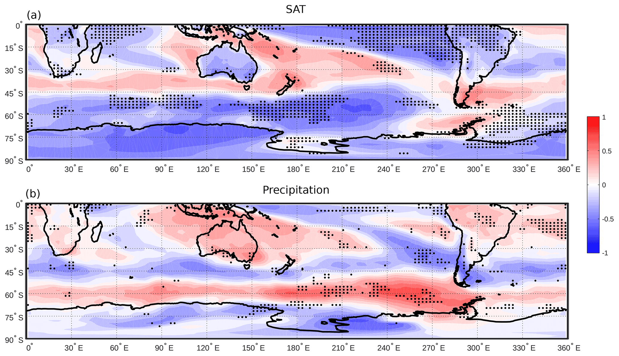
Figure 1 Correlations of annual-mean (January–December) SAT (a) and precipitation (b) from the GFDL CM2.1 model with the model-derived SAM, calculated over 500 years. Black dots show where the correlation of the ERA-Interim reanalysis product with the Marshall SAM index, calculated over a 36 year period from 1979 to 2014, does not fall within the range of the model's 36 year running correlation at each grid cell.

Paleo-proxies are not uniformly sensitive to one season or variable; their sensitivities depend on the region from which they are sourced. For example, a tree ring record constructed by Cullen and Grierson (2009) from south-west Western Australia was shown to be particularly sensitive to austral autumn–winter precipitation. Alternatively, South American tree ring records compiled by Villalba et al. (2012) show sensitivity to summer–autumn precipitation, while New Zealand records appear to be most responsive to summer temperature. In addition, while the proxies are sensitive to SAT or precipitation during one season, the strongest influence of the SAM on these variables may occur during a different season entirely. For example, while the South American tree rings of Villalba et al. (2012) are sensitive to summer–autumn precipitation, the SAM signal is most clearly seen in late spring and winter precipitation in south-eastern South America (Silvestri and Vera, 2009). With this in mind, we employ annual mean (January–December) fields for sea level pressure, surface air temperature, and precipitation for the following reasons: (1) the CMIP5 generation of models (including CM2.1) are less skilful at representing the seasonal variability in the SAM–SAT relationship than they are at representing the annual mean (Marshall and Bracegirdle, 2015); (2) reconstructing the SAM on an annual-mean timescale should smooth out high-frequency noise in the proxies and enhance the signal-to-noise ratio of our reconstructions; and (3) it enables us to simplify the experimental parameter space and focus instead on the impacts of network size and calibration window length rather than seasonal effects.

2.2 Calculation of non-stationarity

A proxy is typically considered non-stationary if its teleconnection to the SAM is changed by a dynamical process rather than stochastic variability (localised weather), such that the signal it records no longer represents changes in the SAM. Here, the SAM teleconnection is modelled via a running correlation between the proxy and the SAM index over a window of 31, 61, or 91 years. We define non-stationary teleconnections following the method of Gallant et al. (2013) and Batehup et al. (2015), such that a proxy is considered non-stationary when the variability in its running correlation with the SAM exceeds what would be expected if the proxy were only influenced by local random noise.

Following on from this, a Monte Carlo approach (van Oldenborgh and Burgers, 2005; Sterl et al., 2007; Gallant et al., 2013) is used to create stochastic simulations of SAT and precipitation at each grid point in the model. These stochastic simulations are created to have the same statistical properties as the original SAT and precipitation data from the CM2.1 simulation. To determine the range of variability expected due to the stochastic processes mentioned previously, 1000 of these time series are created at each grid point according to the following equation from Gallant et al. (2013):

$$\begin{array}{}\text{(1)}& v\left(t\right)=a_{\mathrm{0}}+a_{\mathrm{1}}c\left(t\right)+{\mathit{\sigma }}_v\sqrt{\mathrm{1}-r^{\mathrm{2}}}\left[{\mathit{\eta }}_v\right(t)+\mathit{\beta }{\mathit{\eta }}_v(t-\mathrm{1}\left)\right].\end{array}$$

Here, v(t) is the stochastic SAT or precipitation time series, a₀ and a₁ are regression coefficients representing the stationary teleconnection strength between the SAT or precipitation and the SAM index (c(t)), while the remaining terms represent the noise added to the time series. A red noise, $\left[{\mathit{\eta }}_v\right(t)+\mathit{\beta }{\mathit{\eta }}_v(t-\mathrm{1}\left)\right]$, is added and weighted by the standard deviation σ_v of the local SAT or precipitation time series as well as the proportion of the variance not related to the regression ($\sqrt{\mathrm{1}-r^{\mathrm{2}}}$), where r is the correlation between the SAT/precipitation time series and the SAM index. The red noise is a combination of random Gaussian noise (η_v(t)) and the autocorrelation (β) of the SAT or precipitation time series at a lag of 1 year multiplied by the Gaussian noise (βη_v(t−1)).

The stochastic simulations of SAT and precipitation are used to create a 95 % confidence interval for each grid point of all possible running correlations a time series could have and still be considered to have a stationary teleconnection with the SAM. Therefore, if the time series from our model proxy has a running correlation that falls outside the confidence interval, we consider that proxy to be non-stationary with the SAM in that temporal window, as it is unlikely to be affected by stochastic processes alone. It should be noted that as a 95 % confidence interval is used, non-stationarity will be falsely identified 5 % of the time, hence we define a grid point as non-stationary only if the running correlation falls out of the confidence interval more than 10 % of the time – more than double the 5 % we might expect by chance alone. The running correlations are converted to Fisher Z-scores to ensure they are normally distributed for the calculation of confidence intervals:

$$\begin{array}{}\text{(2)}& Z={\displaystyle \frac{\mathrm{1}}{\mathrm{2}}}\ln \left({\displaystyle \frac{\mathrm{1}+r}{\mathrm{1}-r}}\right),\end{array}$$

where r is the running correlation value.

2.3 Generation of pseudoproxies

SAT and precipitation fields from the model are used to represent climate proxies in the model, as discussed in Sect. 2.1. Rather than being inferred via changes in tree ring growth, these proxies are direct measures of these variables and therefore free of non-climatic noise (von Storch et al., 2009). We do not add noise to increase the realism of these proxies; rather, we assess reconstruction skill and non-stationarity in a “best case scenario” where we assume that the proxy is a perfect analogue for the climate variable it is deemed to represent (SAT or precipitation), similar to the experiments of Dätwyler et al. (2020).

Proxies are randomly selected in accordance with two conditions. Ideally, proxies would be calibrated with the SAM over the full length of the time series (500 years); however, as previously noted, real-world proxies are calibrated over shorter windows of several decades. For each grid point in the model, the time series is split into 10 windows either 31, 61, or 91 years in length, whose midpoints are evenly spaced throughout the 500 years regardless of the overlap or space between them. A proxy may be selected if it is (1) on land in the Southern Hemisphere and (2) has a correlation with the model SAM index of $\left|\mathrm{0.3}\right|$ or greater within the calibration window, after the method of McGregor et al. (2013) and Batehup et al. (2015). A threshold correlation of 0.3 is an arbitrary choice, but it ensures that the proxy represents the SAM to some extent while not being so high that proxies are only sourced from a geographically limited region.

The number of proxies that meet our criteria in each region/window size is shown in Table 1. This approach allows for the possibility that a proxy has a strong correlation with the SAM over the selected calibration window but an insignificant or even reversed correlation over other windows, or indeed the full 500 years. The window sizes were chosen to assess the effect of window length on the resulting skill of the reconstruction. For example, the use of a 61 year calibration window, as opposed to a 31 year one, may decrease the effect of decadal climate variability and its modulation of the pseudoproxy–SAM teleconnection.

Table 1 The range in the number of sites available for use in a SAT or precipitation proxy network in each region and the calibration window size. The range was calculated across the 10 different calibration windows used when creating the network, as discussed in Sect. 2.3.

Reconstructions are computed with a network size of between 2 and 70 proxies, a range typical of past reconstructions with strict selection criteria (e.g. Abram et al., 2014 and Dätwyler et al., 2018). This is done to quantify the dependence of reconstruction skill on network size. 1000 networks are generated for each of the 10 calibration windows for each network size. Each site in each network is randomly selected and unique, while the same site may be included in more than one network. Similarly, all sites in a network are selected based upon correlations over a single window and may therefore be absent from networks calibrated using a different window.

To reconstruct the proxy networks into a single proxy-SAM index, we use the weighted composite plus scale (CPS) method (Esper et al., 2005; Hegerl et al., 2007), similar to that used by Abram et al. (2014). The scope of this study does not include the effects of different reconstruction methods on the skill of the reconstructed index, so we choose to use CPS because it is commonly employed in paleo-reconstructions (PAGES 2k Consortium, 2013; Abram et al., 2014; Batehup et al., 2015; Dätwyler et al., 2018). Using this method, proxies are normalised to have a zero mean and unit standard deviation, and are then weighted according to their correlation with the model SAM over the calibration window before being summed into a single time series. To quantify the skill of the pseudoproxy reconstructions, Pearson correlation coefficients between each normalised SAT/precipitation-derived SAM index and the sea level pressure-derived SAM index over the full 500 years of data are calculated. We define a skilful reconstruction as one that is able to reproduce at least 50 % of the model SAM variability (i.e. r²≥0.5 or $r\ge \sim \mathrm{0.71}$).

To investigate the role that ENSO may play in modulating the pseudoproxy–SAM teleconnection, a correlation coefficient is calculated between the running correlation time series of SAM-SAT/precipitation and the model Nino3.4 (n3.4) index at each grid point. The n3.4 index is chosen due to its optimal representation of the character and evolution of El Niño and La Niña events (Bamston et al., 1997; Trenberth and Stepaniak, 2001). The model n3.4 index is calculated as the sea surface temperature anomaly in the region from 5^∘ N to 5^∘ S and from 170^∘ W to 120^∘ W.

Each SAT and precipitation grid cell is correlated with the SAM over a 31, 61, and 91 year running window, while the n3.4 index is bandpass filtered using the same window size to remove high-frequency variability. The two time series are then correlated over their common interval (500 years minus the window size), with the significance calculated using a reduced degrees of freedom method (Davis, 1976). An additional set of SAM reconstructions are calculated which exclude any proxy whose SAM–proxy running correlation is found to have a significant (p<0.05) correlation to the filtered n3.4 index over the relevant calibration window.

3 Results

The importance of a long calibration window is illustrated in Fig. 2. For example, a true correlation of −0.3 between precipitation and the SAM may become anything ranging from −0.65 to 0.1 when evaluated over a shorter 31 year window (Fig. 2d). However, as the window size increases, it is increasingly likely that the calculated correlation is representative of the true correlation. For example, calibration windows of 61 and 91 years ensure that our proxy's correlation with SAM is always the same sign as it is over the 500 year period (Fig. 2e and f). Also noteworthy is the considerable decrease in the maximum available number of proxies eligible for inclusion in reconstructions when calibrating with a 61 year window rather than a 31 year window (Table 1). A smaller decrease in the proxy pool is seen when lengthening the window from 61 to 91 years.

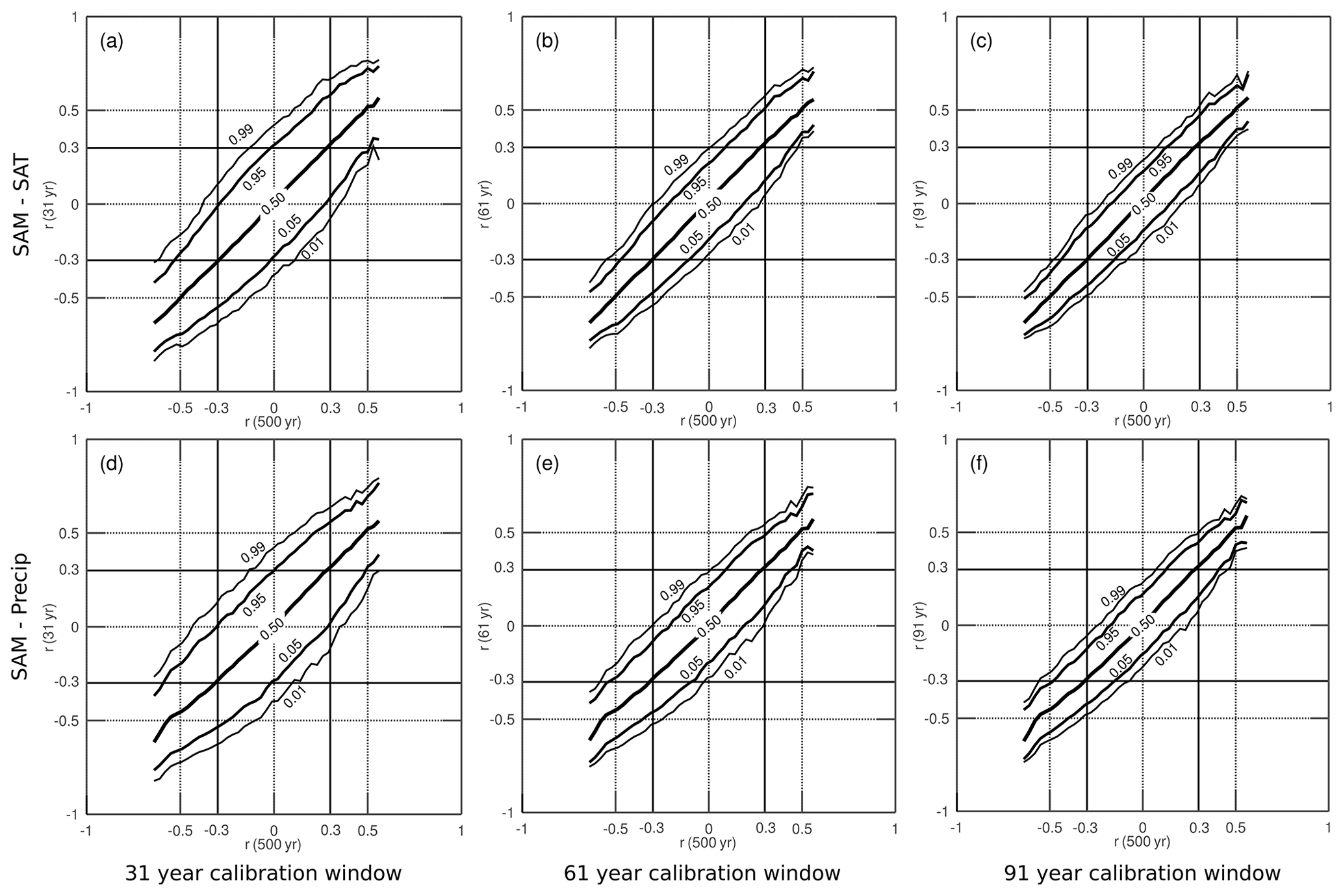
Figure 2 Correlation coefficients between the model SAM index and both SAT (a, b, c) and precipitation (d, e, f) fields. Panels show the probability distribution of a grid point with a certain probability in a 31 year (a, d), 61 year (b, e), and 91 year (c, f) calibration window given the same point's correlation over the full 500 years. This illustrates how a longer calibration window will ensure that the correlation of a point to the SAM within that window will be closer to the “true” correlation calculated over the full 500 years.

3.1 Reconstruction skill

Reconstructions of the SAM often rely heavily on proxies from a very limited geographic location. What follows are several reconstructions, each one utilising proxies from one or more regions which are commonly used to reconstruct the SAM. In the first scenario, shown in Fig. 3a–f, pseudoproxies are sourced from the entire Southern Hemisphere (SH), including Antarctica. The reconstruction skill is displayed as a correlation (y axis) between the pseudoproxy-generated SAM index and the “real” SAM index calculated from sea level pressure (SLP) fields in the model. This is plotted against the number of proxies used to generate the reconstruction (x axis). The ranges of the 5th, 50th, and 95th percentiles represent the use of 10 different calibration windows and show the effect this has on the reconstruction.

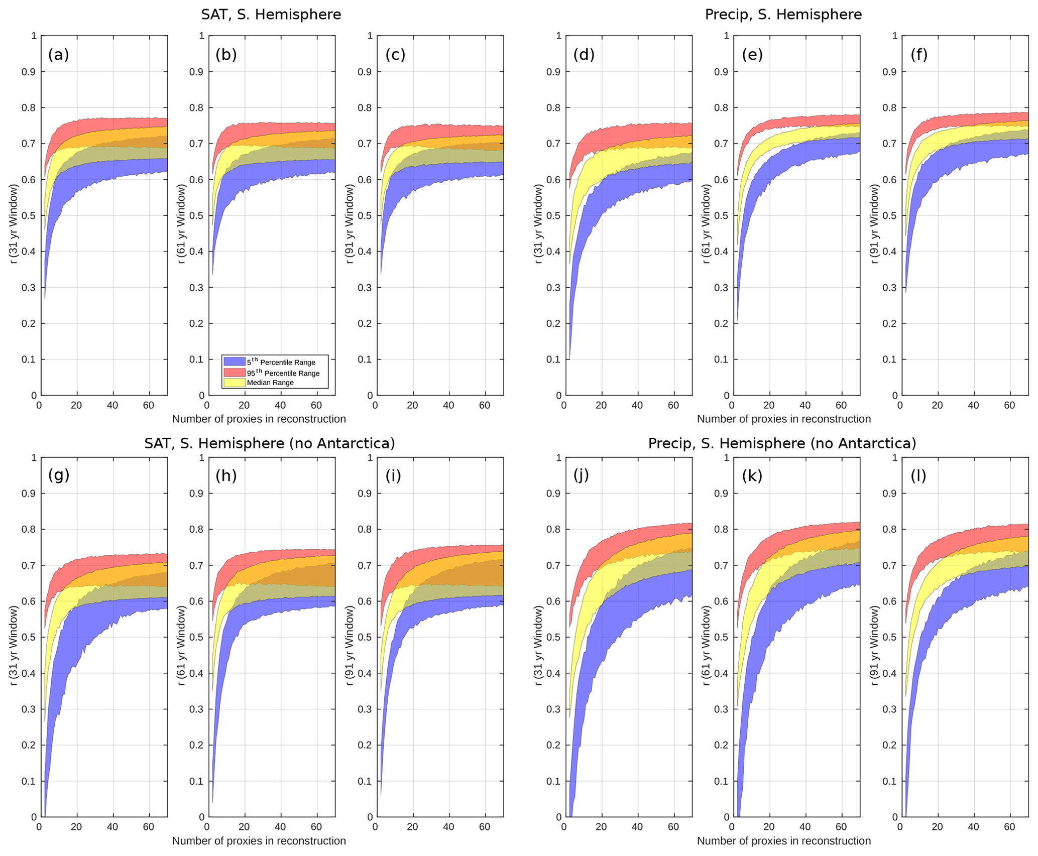
Figure 3 Correlation of the model SAM index (y axis) to the pseudoproxy reconstructions described in Sect. 2.3, plotted here by network size (x axis). Each panel shows the reconstruction skill for the 31, 61, or 91 year calibration window. The three shaded areas show the 5th, 50th, and 95th percentiles, respectively. Their ranges represent the ranges of these percentiles across the 10 different calibration windows for each window/network size. Panels (a)–(c) and (d)–(f) show reconstructions for SAT and precipitation, respectively, are proxies are sourced from the entire Southern Hemisphere. Panels (g)–(i) and (j)–(l) show reconstructions generated using proxies sourced from everywhere but Antarctica, but are otherwise equivalent to (a)–(f).

Results suggest that small proxy networks (2–10 proxies) rarely provide skilful reconstructions of the SAM, even when the calibration window is a relatively large 91 years (Figs. 4 and 5, panels a, e, i; red line), though a greater proportion of precipitation-derived reconstructions are considered skilful across all window sizes. The range in reconstruction skill is smaller for precipitation than for SAT, particularly when longer calibration windows are used, suggesting larger multi-decadal variability in the SAM–SAT teleconnection over time. Maximising the number of records in the proxy network leads to a larger proportion of skilful reconstructions, although for the shortest window of 31 years, the reconstruction skill in the 95th percentile is never greater than r=0.76 for precipitation and r=0.77 for SAT (r² = 0.58 and 0.59, respectively), suggesting that around 60 % of the model SAM variability can be reproduced at most. Minimum values (the lowest r value in the 5th percentile for 70 proxies and the 31 year window) are r=0.62 for SAT and r=0.59 for precipitation, reconstructing 38 % and 35 % of the SAM variability, respectively (Fig. 3a and d).

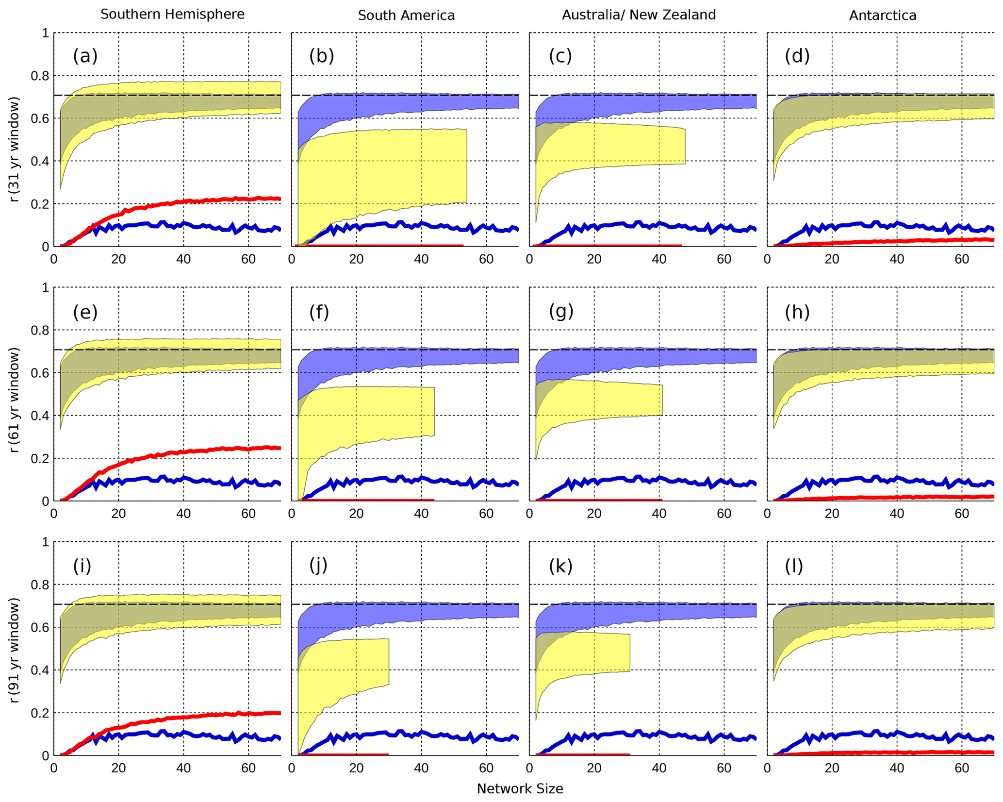
Figure 4 Differing reconstruction skill achieved when using SAT-derived proxies sourced from the entire Southern Hemisphere (a, e, i), South America (b, f, j), Australia and New Zealand (c, g, k), and Antarctica (d, h, l) only. The correlation between a SAT-derived reconstruction and the SAM is plotted on the y axis, while the number of sites used ($n=\mathrm{2}:\mathrm{70}$) in a reconstruction is plotted on the x axis. Shaded regions represent the range between the minimum of the 5th percentile and the maximum of the 95th percentile for each network size across 10 000 reconstructions (described in Sect. 2.3). Each set of regional reconstructions is shaded in yellow, and the end of this yellow region indicates the number of samples available when it is below 70. Each panel also includes the range in skill for reconstructions with sites sourced from the entire Southern Hemisphere and calibrated with a “true” 500 year window (blue shading). The blue line indicates the percentage of true SH reconstructions that meet or exceed our skill threshold of being able to explain 50 % or more of the variability in the SAM. The red line indicates the same thing, but for each regional reconstruction. The dashed black line indicates the r value required to meet our skill threshold.

Figure 5 Differing reconstruction skill achieved when using precipitation-derived proxies sourced from the entire Southern Hemisphere (a, e, i), South America (b, f, j), Australia and New Zealand (c, g, k), and Antarctica (d, h, l) only. The correlation between a precipitation-derived reconstruction and the SAM is plotted on the y axis, while the number of sites used ($n=\mathrm{2}:\mathrm{70}$) in a reconstruction is plotted on the x axis. Shaded regions represent the range between the minimum of the 5th percentile and the maximum of the 95th percentile for each network size across 10 000 reconstructions (described in Sect. 2.3). Each set of regional reconstructions is shaded in yellow, and the end of this yellow region indicates the number of samples available when it is below 70. Each panel also includes the range in skill for reconstructions with sites sourced from the entire Southern Hemisphere and calibrated with a “true” 500 year window (blue shading). The blue line indicates the percentage of true SH reconstructions that meet or exceed our skill threshold of being able to explain 50 % or more of the variability in the SAM. The red line indicates the same thing, but for each regional reconstruction. The dashed black line indicates the r value required to meet our skill threshold.

The range in reconstruction skill presented in Fig. 3 indicates that even when the network size is maximised and a long window is selected, simply calibrating during a different period can change the skill of the resulting reconstruction. It is noteworthy that increasing the calibration window length does not necessarily increase the maximum possible skill of the resulting reconstruction, but rather leads to a reconstruction converging towards the skill of a so-called “true” reconstruction. This true reconstruction utilises the entire time span of our data for calibration, which is 500 years here, and shows the actual ability of these proxies to reconstruct the SAM. This convergence is visible for the SH SAT reconstructions (Fig. 4a, e, and i), where a longer calibration window does not increase the 95th percentile of reconstruction skill nor necessarily increase the proportion of skilful reconstructions (Fig. 4e and i; red lines). In other words, a longer calibration window will more realistically represent a proxy's relationship with the SAM, but, as a result, it may decrease the skill of the reconstructed SAM.

As Antarctica represents a large percentage of the available proxies (Table 1), reconstructions are included for proxies sourced from the entire Southern Hemisphere other than Antarctica to ensure they are not disproportionately impacting the skill of our reconstructions. The Antarctic-free SAT reconstructions are less skilful for the 31 and 61 year windows with a larger range in r. Note that most of the 95th percentile (Fig. 3g, h, i – red shading) is below the r²>0.5 skilful threshold, as opposed to reconstructions with Antarctic sites. Antarctic-free precipitation reconstructions typically see an increase in maximum skill but a similar increase in the range (Fig. 3i–l). The contrasting effects of Antarctica could be due to Antarctic precipitation having a generally weak correlation with the model SAM, while SAT shows strong negative correlation with the SAM continent-wide (Fig. 1); by removing these points, we lose skill in the SAT-derived reconstructions and increase skill in the precipitation-derived reconstructions.

Data from different regions may also act to increase or decrease the skill of reconstructions. Figures 4 and 5 illustrate the skill of each regional reconstruction in comparison to the SH one. In addition, comparisons are made to a reconstruction with a true calibration window of 500 years, showing the actual range in skill that the pseudoproxies can produce. Southern Africa was excluded from this analysis, as too few grid cells met our criteria for reconstruction. When we utilise records from individual regions, the reconstructive skill of the proxy network is significantly reduced. Reconstructions for the Australia–New Zealand region (Figs. 4 and 5c, g, k), South America (Figs. 4 and 5b, f, j), and Antarctica (Figs. 4 and 5d, h, l) all show reduced reconstructive skill when compared with the entire SH network (Figs. 4 and 5a, e, i), with Antarctica being the only individual region capable of generating any skilful reconstructions. In general, then, reconstructing the SAM using pseudoproxies in CM2.1 is most successful when we maximise network size and source sites from as many geographical regions as possible, particularly at longer calibration windows, where the proxy pool becomes too small for a full network in many regions. The exceptions here are precipitation-based reconstructions, where leaving out Antarctica improves reconstruction skill.

When comparing proxy types, there are significantly more skilful precipitation-derived reconstructions than for SAT, and this is true across all window sizes for the Southern Hemisphere-wide reconstructions (Figs. 4 and 5a, e, i). In particular, when using a 61 or 91 year window, 89 % and 91 % of SH precipitation reconstructions are considered skilful, respectively (with a network size of 70) (Fig. 5e and i), and an increase in window size increases the proportion of skilful reconstructions (Fig. 5a, e, i; red line). In contrast, SAT reconstructions calibrated with 61 and 91 year windows only produce skilful reconstructions 25 % and 20 % of the time, respectively (Fig. 4e and i). Most striking here is that a longer calibration window both decreases the 95th percentile skill and the proportion of SAT-derived reconstructions that can be considered skilful. But this is reasonable when we see that, at best, 11 % of true SAT reconstructions are skilful and have a lower maximum skill for the 95th percentile (Fig. 4e and i). This result indicates that shorter calibration windows are sufficiently susceptible to climatic noise or modulation that they are producing reconstructions with spuriously larger reconstruction skill. It is also worth noting that the reduction in the reconstruction skill range visible for the 61 and 91 year windows relative to the 31 year window will necessarily be in part due to the overlapping of the 10 calibration windows over the 500 years of model data. With a longer data set, the lack of such an overlap would almost certainly result in this spread being larger.

While increasing the number of sites used in each reconstruction does not necessarily improve the maximum 95th percentile skill after approximately n=10, it does narrow the range of possible reconstruction skill (Figs. 4 and 5a, e, i; note the yellow envelope converging on the blue with increasing window size). Figures 4a, e, i give the impression that our reconstructions outperform the true reconstructions, but they have virtually the same maximum skill at each network size. This apparent incongruence occurs due to the probability distribution of reconstruction skill for our true proxies being far narrower than for the reconstructions with varying window length, resulting in the 95th percentile having a generally lower value for each network size.

3.2 Mapping non-stationarity

In this section, we examine whether certain regions are more or less non-stationary to the SAM, which would contribute to these regions being better or worse than others at reconstructing the SAM. Figure 6 shows the number of non-stationary years at each grid point for SAT (a) and precipitation (b) as defined in Sect. 2.2. Grid points with running correlations that fall outside the 95 % confidence interval of stochastic variability more than 10 % of the time are highlighted with solid contours; we define these regions as non-stationary. For SAT, 6 % (31 year window) and 11 % (61 and 91 year windows) of the land cells are non-stationary; for precipitation, 7 % (31 year window) and 14 % (61 and 91 year windows) are.

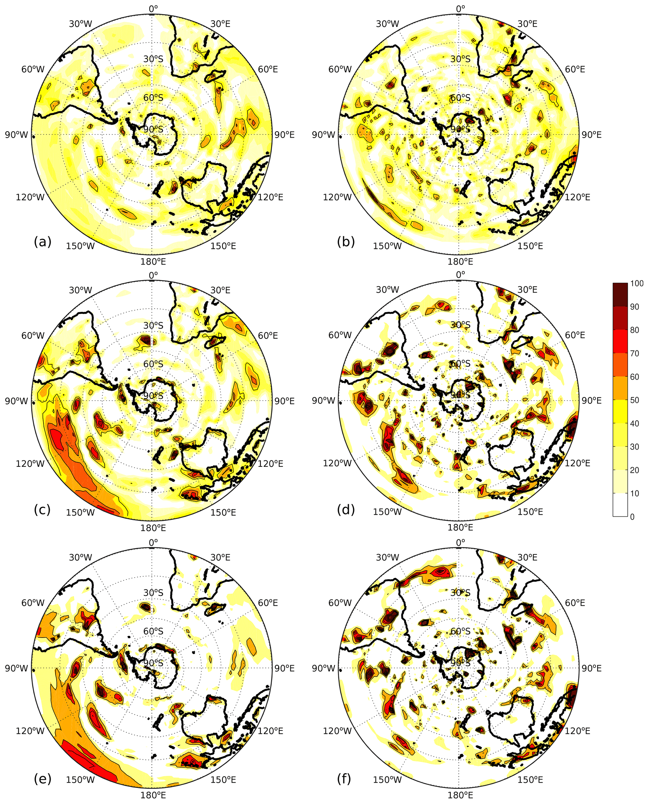
Figure 6 Number of years at each grid point where the 31 year (a, b), 61 year (c, d), and 91 year (e, f) running correlation between SAT (a, c, e) or precipitation (b, d, f) and the model SAM falls outside the 95 % stationarity confidence interval (Sect. 2.2). As per our definition of non-stationarity, regions which fall outside this interval 10 % of the time or more (≥47, 44, and 41 years for the 31, 61, and 91 windows, respectively) are highlighted with solid black contours and are considered to be non-stationary.

Depending on the length of the calibration window, different patterns of non-stationarity appear, particularly for SAT. Aside from three small regions in south-east Australia, central South America, and the Queen Elizabeth Range in Antarctica, there are almost no land sites that can be considered non-stationary when using a 31 year running correlation for SAT. It is also noteworthy that these non-stationary regions (as calculated using the 31 year running correlation) appear to fall, on average, in regions where correlations are weaker (though still significant at p<0.1 when r>0.08) over the full 500 years (Fig. 1a). The same is also broadly true for precipitation, where large regions of non-stationary points do occur but fall in regions of weaker or zero correlation with the SAM, particularly in East Antarctica (Fig. 1b). It is worth noting, however, that despite not meeting the requirement of being classified as non-stationary, large regions of the Southern Hemisphere land surface show modulation of the SAM–proxy teleconnection (Fig. 6, yellow regions).

To better illustrate the impact of non-stationary proxies on reconstructions, Fig. 7a compares the skill of our SH reconstructions with the percentage of non-stationary proxies in each. The effect of non-stationary sites is negative in all but one instance. Correlations are typically stable with network size and are relatively weak, with mean r² values of 0.03. Reconstructions calibrated with a 31 year window are outliers, both of which see a slight increase in skill with larger network sizes. In particular, the positive relationship observed for the precipitation reconstructions (Fig. 7a and b, purple line) suggests that these proxies provide a net benefit to the reconstructions they are part of, despite their non-stationary nature. SAT reconstructions calibrated over 61 and 91 years are noteworthy as the impact of non-stationary sites is larger (r² = 0.19 for 70 proxies calibrated over 91 years) and increases with network size when compared to other scenarios (Fig. 7a and b, yellow line).

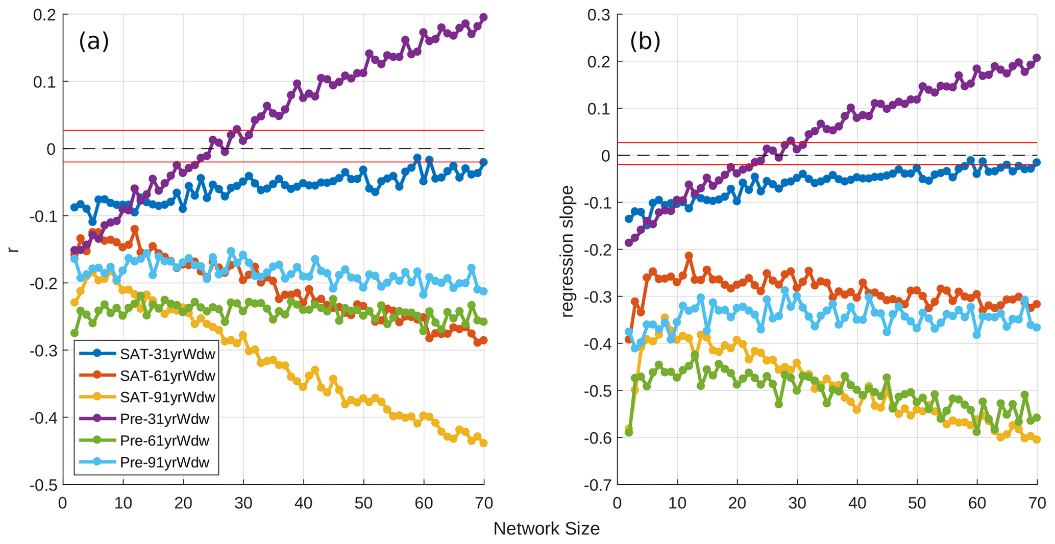
Figure 7 Correlation (y axis) between the skill of a given reconstruction and the percentage of non-stationary proxies it contains (a), plotted as a function of network size. (b) is the same as panel (a), but the y axis shows the regression slope. Calculations are over 10 000 reconstructions for each network size. r=0 is plotted as a dashed black line. All correlations are significant to at least p<0.05, other than in the region bounded by the two red lines about r=0.

The negative relationship between reconstruction skill and non-stationarity belies the chances of producing a reconstruction with a large proportion of non-stationary proxies. Figure A1c and d demonstrate that, for a network size of 70, the most likely proportion of non-stationary proxies in a reconstruction is ∼5 %, and even this constitutes only 10–15 % of reconstructions. While increasing the calibration window results in a larger number of non-stationary sites in the reconstruction, a sufficiently large proxy network minimises the probability that these non-stationary sites will represent a significant proportion of the network. In summary, there is a weak negative relationship between the proportion of non-stationary proxies in a reconstruction and its skill, but this impact is not felt by the majority of our reconstructions.

3.3 Modulation of the SAM–proxy teleconnection

While few terrestrial cells qualify as non-stationary based on the definition in Sect. 2.2, there is still considerable variance in the teleconnection strength between SAM and SAT/precipitation over the 500 years of the simulation (Fig. 8). While this could be due to climatic noise, it is not unreasonable that other modes of climatic variability – in particular ENSO – may be modulating this teleconnection (Silvestri and Vera, 2009; Fogt et al., 2011; Dätwyler et al., 2020). The regions from which we source our proxies, such as Australia/New Zealand and South America, are strongly impacted by ENSO, with its teleconnections visible in both temperature and precipitation fields (Davey et al., 2014). The following section will examine which regions show the most variance in proxy–SAM teleconnection and whether these regions appear to be influenced by the model ENSO.

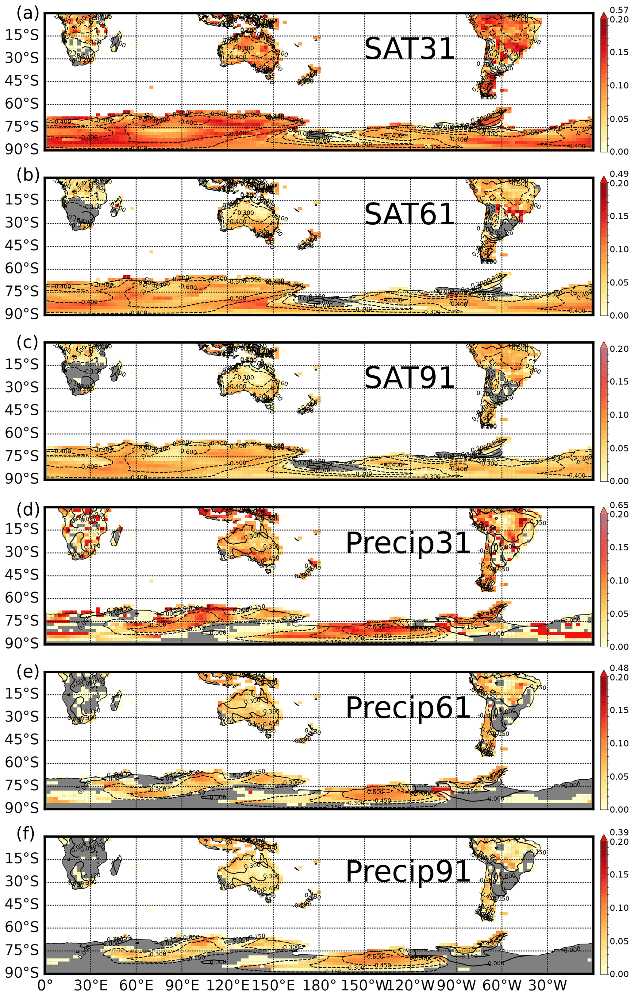
Figure 8 One standard deviation of the correlation of either the model SAT (a–c) or the precipitation (d–f) with the model SAM index over the 10 calibration windows. Panel (a) shows values for the ten 31 year calibration windows for SAT. Panels (b) and (c) show values for the ten 61 and 91 year windows, respectively. Panels (d), (e) and (f) are the same, but for precipitation. Maximum values on the colour bars for panels (a), (b), (d), (e), and (f) indicate the colour of several outliers in the data. Grey regions indicate cells that did not meet the minimum correlation criteria ($r\ge \left|\mathrm{0.3}\right|$) over any windows, meaning that no standard deviation could be calculated. Dashed contours show the model SAM–SAT (a–c) and SAM–precipitation (d–f) 500 year correlation fields from Fig. 1.

Variations in SAM teleconnection strength for SAT proxies show considerable variance in Antarctica, northern and southern South America, and, for the 31 and 61 year windows, parts of Australia and New Zealand (Fig. 8a–c). Distinct regions of higher teleconnection variance in Antarctica are typically in regions of high SAM–SAT correlation over the full 500 years (Fig. 8a–c; dashed contours), with this variance decreasing as we move to a 91 year calibration window. Further to this, variance is typically low for regions with a small 500 year r value.

Significant correlations between the running correlations of SAM–SAT and the filtered n3.4 index can be seen over much of Western Antarctica, south-eastern Australia, and parts of South America (all windows, Fig. 9a–c), while significant correlations are also seen in East Antarctica in the 31 year window. ENSO's modulating influence can be seen to vary depending on both the strength of the underlying SAM–proxy correlation as well as the calibration window length (Fig.  10). For the 31 year window, the regression coefficient between ENSO and the SAM–SAT running correlation is relatively low, clustering predominately between 0.2 and 0.4 (Fig. 10a), and it generally decreases if a site has a stronger correlation with SAM over the full 500 year period. A similar relationship is visible for the 61 year window, but the regression coefficients are slightly larger (∼0.25–0.5), and a decrease in the ENSO regression coefficient with increasing SAM–SAT r is less apparent. The 91 year window sees this relationship disappear altogether, with relatively large (∼0.6–0.8) regression coefficients independent of the SAM–proxy correlation (Fig. 10c and f). This is of lesser consequence, however, as most sites show little variance in SAM–SAT teleconnection at this longer window length (Fig. 8c; most regions have an r_std<0.1), despite ENSO potentially being responsible for 50 % or more of this variance (Fig. 10c). Furthermore, any impact of ENSO on the SAM–SAT teleconnection can be reduced with a longer calibration window, as the number of land points (SAM–SAT running correlation) that are significantly correlated with the filtered n3.4 index decreases as the window length increases (i.e. this is, respectively, 30 %, 24 %, and 15 % for the 31, 61, and 91 year windows).

Figure 9 Correlation between the (a) 31 year, (b) 61 year, and (c) 91 year SAM–SAT running correlation at each grid cell and the model-derived n3.4 index. The n3.4 index is filtered with a corresponding 30, 60, or 90 year filter. Hatched regions indicate p<0.05.

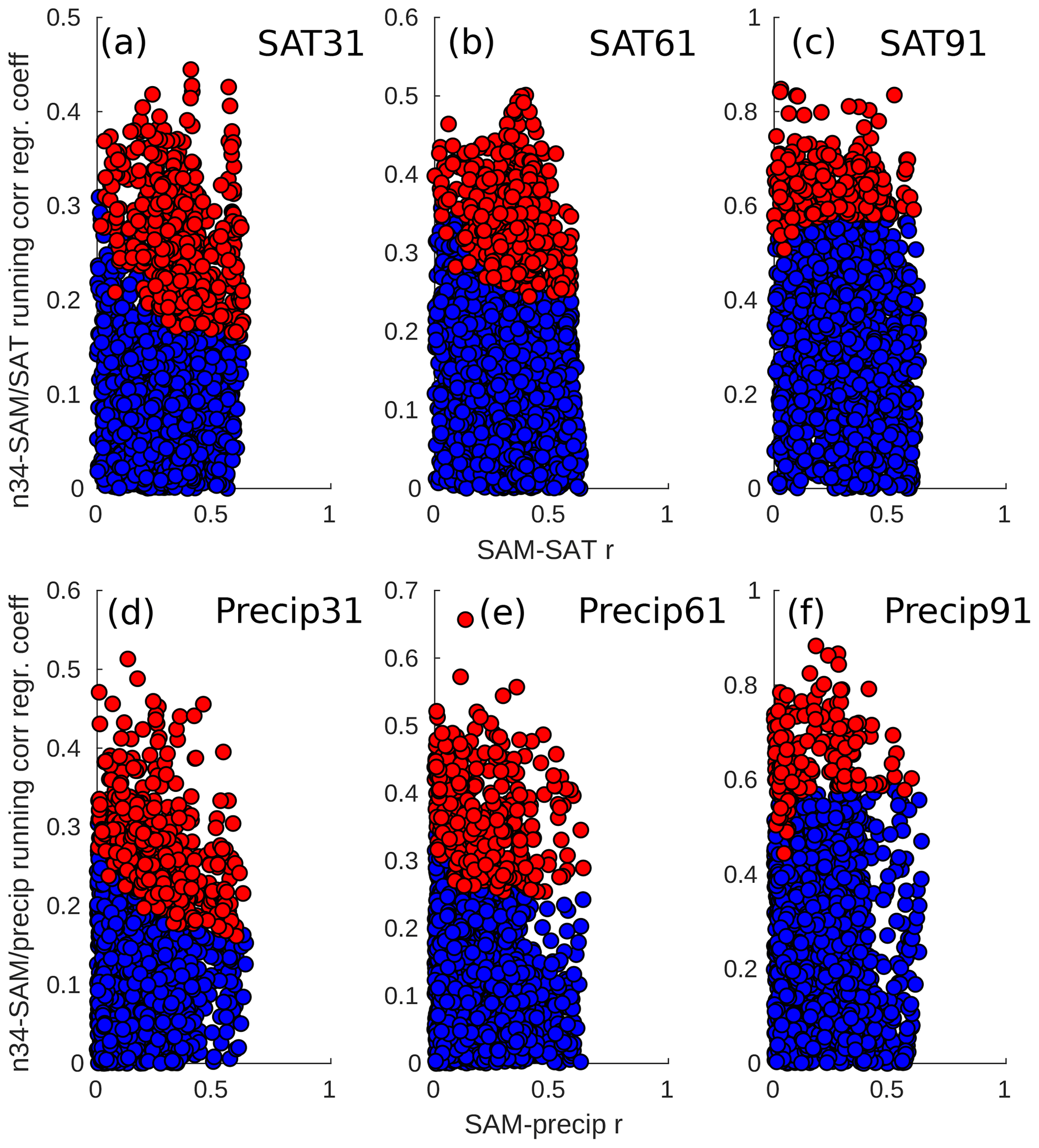
Figure 10 Scatter plots of the regression slopes from the significant (red) and non-significant (blue) land points shown in Figs. 9 and 11 against the 500 year correlation coefficient between the SAM and either the SAT (a, b, c) or the precipitation (d, e, f). Both the SAM–proxy running correlations for each cell and the n3.4 index are standardised prior to the regression calculation. Note that the vertical scale varies depending on the panel.

For precipitation, teleconnection strength is less variable, and only parts of Australia, Indonesia, and the Ross Ice Shelf/Marie Byrd Land in Antarctica show large changes (Fig. 8d–f). Correlation of this precipitation teleconnection variance with the model n3.4 index reveals few regions of significant ENSO influence (Fig. 11), and little coherent spatial structure is observed for this correlation. The magnitude of the impact of ENSO on the SAM–precipitation teleconnection (Fig. 10d, e, f) is similar to the magnitude of the impact of ENSO on the SAM–SAT teleconnection. The number of grid cells impacted by ENSO is fewer than that for SAT, with the running correlation of SAM to precipitation being significantly correlated with n3.4 in 21 %, 16 %, and 8 % of land cells for the 31, 61, and 91 year windows.

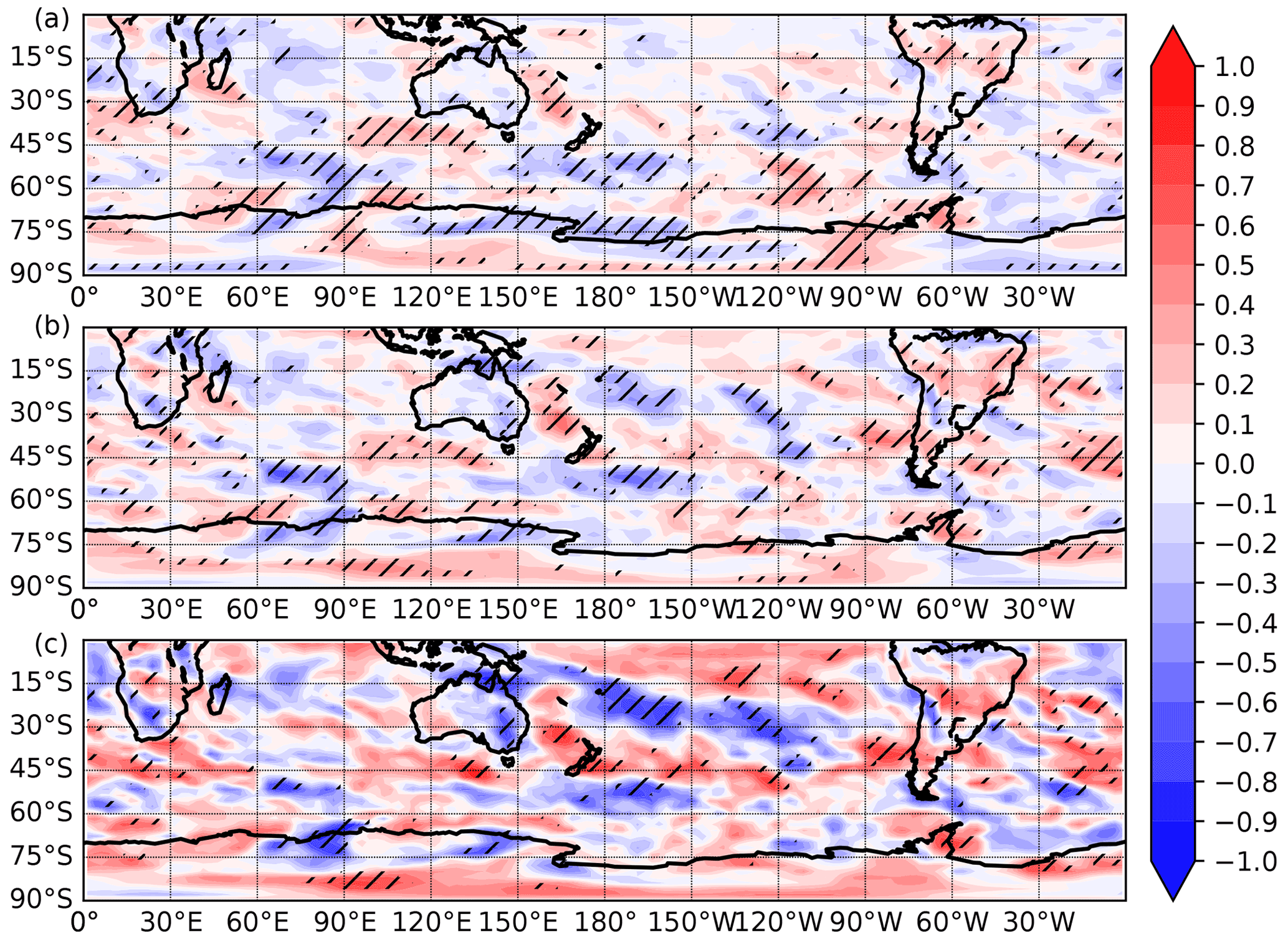
Figure 11 Correlation between the (a) 31 year, (b) 61 year, and (c) 91 year SAM–precipitation running correlation at each grid cell and the model-derived n3.4 index. The n3.4 index is filtered with a corresponding 30, 60, and 90 year filter. Hatched regions indicate p<0.05.

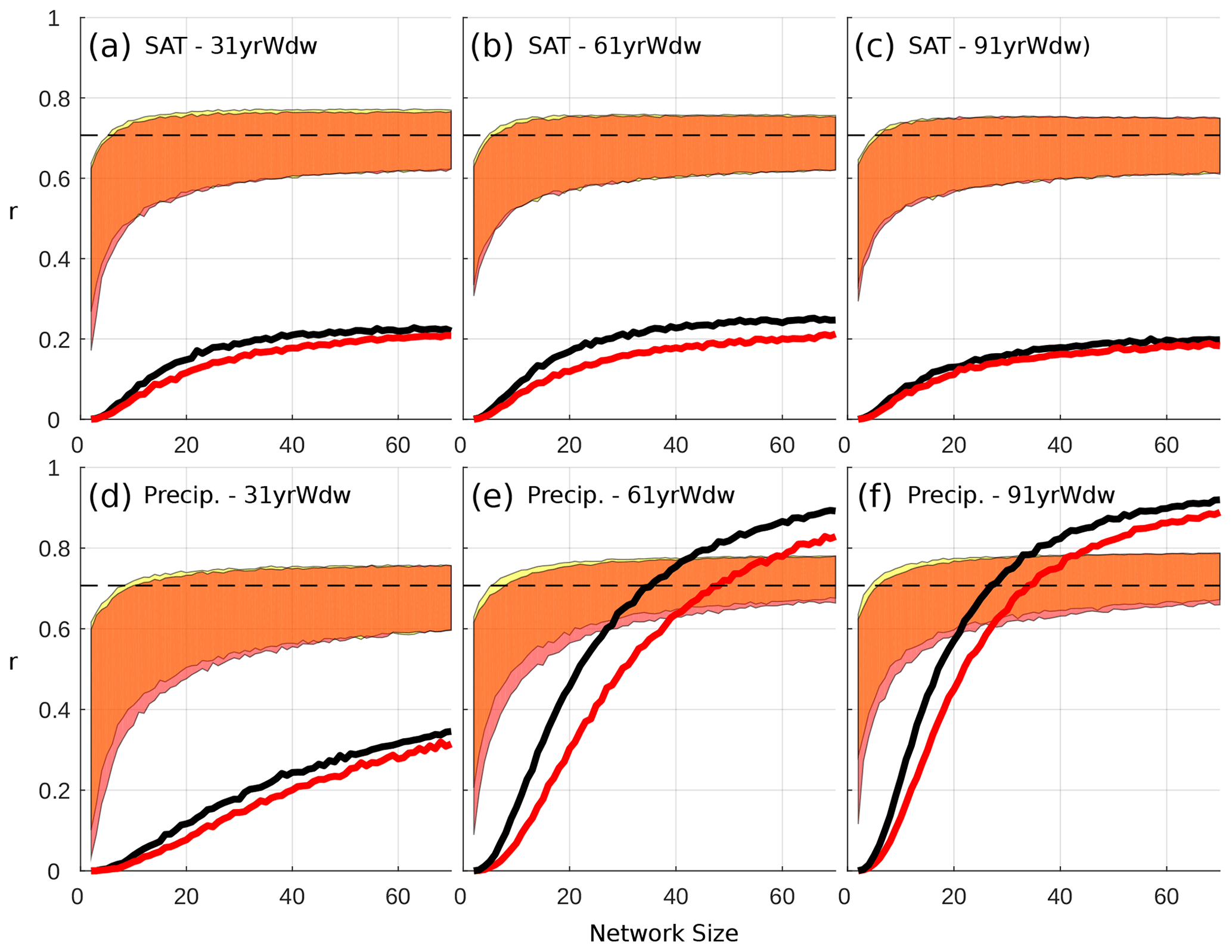
Figure 12 Differing reconstruction skill achieved when sourcing proxies from the entire Southern Hemisphere (yellow envelopes) and the entire Southern Hemisphere, excluding proxies whose teleconnections with SAM have a significant (p<0.05) correlation with ENSO (hatched regions in Figs. 9 and 11; red envelope). The correlation between a SAT-derived or precipitation-derived reconstruction and the SAM is plotted on the y axis, while the number of sites used ($n=\mathrm{2}:\mathrm{70}$) in a reconstruction is plotted on the x axis. Shaded regions represent the range between the minimum of the 5th percentile and the maximum of the 95th percentile for each network size across 10 000 reconstructions (described in Sect. 2.3). The black lines indicate the percentage of SH reconstructions (yellow envelope) that meet or exceed our skill threshold of being able to explain 50 % or more of the variability in the SAM. The red line indicates the same thing, but for those reconstructions that exclude ENSO-sensitive proxies (red envelope). The dashed black line indicates the r value required to meet our skill threshold.

Removing these ENSO-sensitive proxies from our SH-wide reconstructions has a small but negative impact on the proportion of skilful reconstructions we are able to produce for both SAT and precipitation (Fig. 12). Their absence also reduces the minimum skill values for the 5th percentile for all precipitation-derived reconstructions across all network sizes (Fig. 12d, e, f). A smaller effect is visible for SAT-derived reconstructions calibrated with a 31 year window, but only for smaller network sizes. Given the minimal extent to which ENSO appears to modulate the proxy–SAM relationship, removing these proxies – which may otherwise enhance the regional diversity of a network – results in a net degradation of the signal-to-noise ratio in our reconstructions. On the other hand, reconstructions using only ENSO-sensitive proxies (not shown) also result in lower skill, although it is unclear what role ENSO plays due to the vastly reduced pool of proxies we can sample from in this scenario.

4 Discussion and Conclusions

In this study, we use the CM2.1 coupled climate model to examine the limits to SAM reconstruction skill, including the impact of regional biases in the sourcing of proxy records as well as the impact of non-stationary proxy teleconnections. Reconstructions derived from model SAT and precipitation fields and calibrated over a 31 year window are able to – at best – replicate 56 % and 58 % of the SAM variance, respectively, comparing favourably to a “true” reconstruction whose proxies are calibrated over the full 500 year interval (Figs. 4 and 5). This suggests a possible upper limit to the variance an annual-mean SAM reconstruction can reproduce of ∼60 %.

Assessing the skilfulness of our reconstructions, where skilfulness is defined as being able to reproduce ≥50 % of the SAM variance over the full 500 years, reconstructions derived from precipitation performed best (Fig. 3), with a maximum of 91 % of the reconstructions being reported as skilful (91 year window, 70 proxies) and exhibiting less spread due to the variability of the teleconnection between precipitation and the SAM (Fig. 8). SAT-derived reconstructions perform poorly by comparison, with only a maximum of 25 % of the reconstructions qualifying as skilful (61 year window, 70 proxies). It is worth noting that this result remains consistent when examining a different measure for skill. If we consider the median root mean square error (RMSE), precipitation-derived reconstructions perform better overall (minimum RMSE of 0.91 for SAT and 0.90 for precipitation; Fig. A2). As with our threshold skill score, the RMSE shows that skill is maximised by utilising a large proxy network and a longer calibration window of 61 or 91 years, though the difference in skill between SAT and precipitation is smaller.

Both SAT-derived and precipitation-derived reconstructions are most skilful when proxies are selected from a geographically broad region, while regional reconstructions – with the exception of Antarctica – fail to produce any skilful reconstructions. This is likely due to each region being affected by localised climatic noise, which becomes a systematic source of error in the reconstruction. With larger datasets from different regions, this noise cancels out, and the signal we seek to reconstruct is more clearly visible.

Increasing the calibration window does not increase the chance of producing a more skilful reconstruction. It does, however, along with maximising the number of proxies, cause the range of reconstruction skill to converge on the skill of our true proxy reconstructions (blue envelopes, Figs. 4 and 5). It should be noted that this will be due in part to our correlation requirement of $r\ge \left|\mathrm{0.3}\right|$ for proxies, which imposes a progressively more rigorous selection criterion for longer calibration windows. Adding more sites to a reconstruction has limited benefit in terms of the maximum skill it can achieve, with values largely plateauing at a network size of ∼20. Minimum skill, however, improves for increases in network size all the way up to and including 70 proxies (Fig. 3). This increase in skill in turn acts to increase the proportion of skilful reconstructions for a given window size.

There is low-frequency variability in the teleconnections between our pseudoproxies and the SAM that cannot be explained by climatic noise (stochastic variability). CM2.1 simulates, at maximum, 14 % of the land points as being non-stationary as defined by Gallant et al. (2013) (using precipitation as a proxy and a 61 or 91 year running window), although the odds of creating a proxy network with a high proportion of non-stationary sites remains relatively low (Fig. A1). Non-stationary proxies, as defined here, do not seem to modulate SAM–proxy teleconnection strengths or impact on reconstructions greatly, as emphasised by the weak relationship between reconstruction skill and the number of non-stationary proxies in a reconstruction (Fig. 7a). The exceptions are SAT-derived reconstructions with a longer calibration window (61 or 91 years), suggesting that at larger network sizes, care should be taken to minimise the proportion of non-stationary proxies. While assessing the stationarity of a proxy–SAM correlation is more difficult in the real world, we suggest that multiple methods be employed where possible, such as in Dätwyler et al. (2018).

It is not unreasonable to suspect that ENSO may be contributing to proxy–SAM teleconnection variance. Dätwyler et al. (2020) identify a highly variable but centennial-average r of −0.3 between austral summer ENSO and SAM reconstructions over the last millennium. Their pseudoproxy experiments using a CESM1 ensemble show significant changes in SAT during periods of large negative SAM–ENSO correlation (their Fig. 4, bottom left panel). The pattern is similar to our results (Fig. 9a), with regions of significant correlation over much of Antarctica and three regions in the Southern Ocean centred on roughly 60^∘ E, 150^∘ E, and 60^∘ W. Rather than excluding proxies for which the teleconnection with the SAM is significantly correlated with ENSO, we can minimise the impact of ENSO simply by calibrating over a longer window, thus ensuring that, while ENSO may impact these proxies, the variance of their teleconnections with the SAM will be small. Its greater impact at longer windows (Fig. 10) is therefore minimised as the variance of the proxy–SAM teleconnection is smaller (Fig. 8).

As we use only one integration from a single model, it is worth discussing the performance of CM2.1. Its representation of the SAM is good with respect to similar models (Karpechko et al., 2009; Marshall and Bracegirdle, 2015; Bracegirdle et al., 2020), though it does have some biases which may impact the results presented here. For instance, when compared to observations and reanalysis, there is a small equatorward bias in the Southern Hemisphere westerlies in CM2.1, but the spatial structure and amplitude of SLP anomalies associated with these winds, and therefore the SAM, are well simulated (Delworth et al., 2006). These comparisons are encouraging, particularly considering the multi-decadal changes in the teleconnections that have been observed from in-situ temperature and precipitation measurements (see Silvestri and Vera, 2009, Fig. 1; Gillet et al., 2006, Fig. 1). Furthermore, we may expect that the expression of the model SAM in the SAT and precipitation fields in our control simulation may not be identical to that found in observations, given the significant positive trend in the SAM over the last five decades and potentially accounting for some of the model–data discrepancy.

A caveat of this study is our use of annual mean data rather than seasonal fields. This is a distinction from previous real-world reconstructions utilising tree ring records (Zhang et al., 2010; Villalba et al., 2012; Abram et al., 2014; Dätwyler et al., 2018), which are not only more sensitive to the SAT or precipitation in a particular season but also combine these with other proxies such as ice cores (Zhang et al., 2010; Abram et al., 2014; Dätwyler et al., 2018), corals (Zhang et al., 2010), and lake sediments (Abram et al., 2014; Dätwyler et al., 2018), each of which may be more or less seasonally sensitive to multiple climatological fields. In addition, many proxies such as tree rings (Cullen and Grierson, 2009; Villalba et al., 2012) have been shown to have a lag relationship with SAM from the previous year, which is also not accounted for in this study. The “perfect” pseudoproxy experiments of Dätwyler et al. (2020) for an austral summer SAM show similar reconstruction skill to our results (an average 31 year running correlation of ∼0.7–0.8 for their ensemble mean), which (even though the methods of this study are not analogous to theirs) supports the conclusion that proxy-derived reconstructions of the SAM in a model framework can, at best, reproduce 50 %–60 % of the SAM variance on an annual timescale. Finally, the results we present here are derived from a control simulation, and the uncertainties in our reconstructions represent noise internal to the climate system. This is in direct contrast to real-world reconstructions, which have the bad fortune of requiring proxies to be calibrated over a period with a significant anthropologically forced trend in the SAM. We would expect this to increase the uncertainty in reconstructions, and any future model-based verification of real-world reconstructions would need to address this problem.

Most importantly, our results confirm that calibrations of paleo-data to instrumental records over brief time periods can result in misleading teleconnection strengths. The large range in reconstruction skill due to the use of multiple calibration windows suggests that real-life proxy records may provide a misleading representation of reconstructed SAM variability due to this non-stationary behaviour, particularly when the reconstruction network constitutes fewer than 20 proxies. For a SAT-derived, Southern-Hemisphere-wide reconstruction, a longer calibration window minimises this uncertainty but does not necessarily result in a more skilful reconstruction. Rather, the reconstructions converge on the “true” skill that these proxies provide. The use of teleconnection stability screening, as applied in Dätwyler et al. (2018), is an important step in the right direction, and should be utilised alongside correlation “skill” scores and other validation statistics to assess the reliability of a reconstruction. The lack of long-term observational data makes it difficult to circumvent this problem, but climate models which have demonstrated realistic dynamical mechanisms may aid us in calculating the uncertainty of these calibrations in the future.

Appendix A

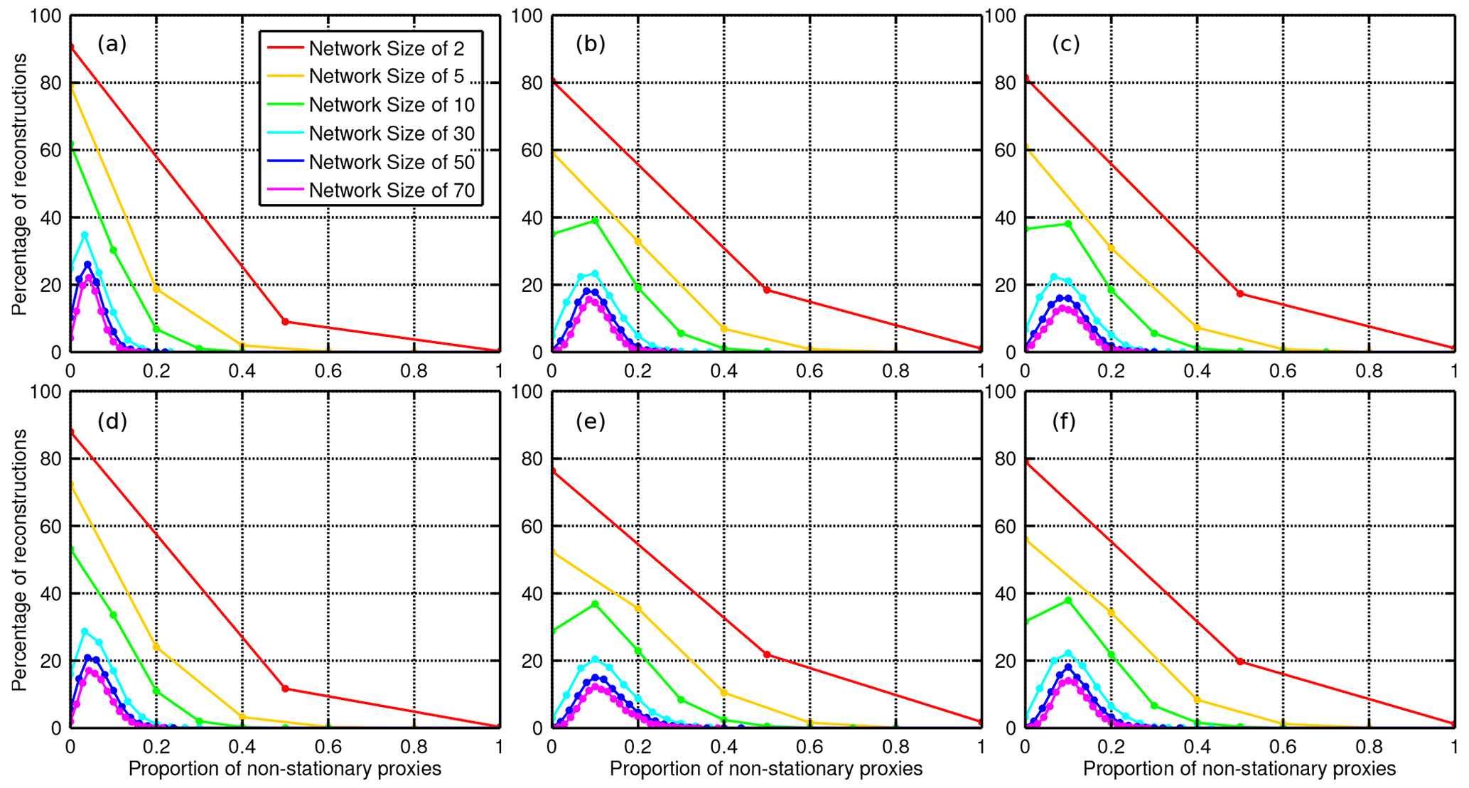
Figure A1 The chance of creating a SAM reconstruction (y axis) with a certain proportion of non-stationary proxies (x axis), as calculated from 10 000 reconstructions for each network size. Panels show the probabilities for 31 year (a, d), 61 year (b, e), and 91 year (c, f) calibration windows. Panels (a)–(c) and (d)–(f) show reconstructions based on SAT and precipitation data, respectively.

Figure A2 Median root mean square error across the 10 000 reconstructions calculated for each network size for SAT-derived (a, b, c) and precipitation-derived (d, e, f) reconstructions. Results are displayed for the 31 year (a, d), 61 year (b, e), and 91 year (c, f) calibration windows. Data is displayed for reconstructions derived from the entire southern hemisphere (SH – blue line), Antarctica only (AA only – red line), Australia and New Zealand (AuNZ – yellow line), and South America (SA – purple line).