the Creative Commons Attribution 4.0 License.
the Creative Commons Attribution 4.0 License.
 | 26 Aug 2021
Significance of uncertain phasing between the onsets of stadial–interstadial transitions in different Greenland ice core proxies
Niklas Boers
Different paleoclimate proxy records evidence repeated abrupt climate transitions during previous glacial intervals. These transitions are thought to comprise abrupt warming and increase in local precipitation over Greenland, sudden reorganization of the Northern Hemisphere atmospheric circulation, and retreat of sea ice in the North Atlantic. The physical mechanism underlying these so-called Dansgaard–Oeschger (DO) events remains debated. A recent analysis of Greenland ice core proxy records found that transitions in Na+ concentrations and δ18O values are delayed by about 1 decade with respect to corresponding transitions in Ca2+ concentrations and in the annual layer thickness during DO events. These delays are interpreted as a temporal lag of sea-ice retreat and Greenland warming with respect to a synoptic- and hemispheric-scale atmospheric reorganization at the onset of DO events and may thereby help constrain possible triggering mechanisms for the DO events. However, the explanatory power of these results is limited by the uncertainty of the transition onset detection in noisy proxy records. Here, we extend previous work by testing the significance of the reported lags with respect to the null hypothesis that the proposed transition order is in fact not systematically favored. If the detection uncertainties are averaged out, the temporal delays in the δ18O and Na+ transitions with respect to their counterparts in Ca2+ and the annual layer thickness are indeed pairwise statistically significant. In contrast, under rigorous propagation of uncertainty, three statistical tests cannot provide evidence against the null hypothesis. We thus confirm the previously reported tendency of delayed transitions in the δ18O and Na+ concentration records. Yet, given the uncertainties in the determination of the transition onsets, it cannot be decided whether these tendencies are truly the imprint of a prescribed transition order or whether they are due to chance. The analyzed set of DO transitions can therefore not serve as evidence for systematic lead–lag relationships between the transitions in the different proxies, which in turn limits the power of the observed tendencies to constrain possible physical causes of the DO events.
- Article
(2753 KB) - Full-text XML
-
Supplement
(45 KB) - BibTeX
- EndNote


In view of anthropogenic global warming, concerns have been raised that several subsystems of the earth's climate system may undergo abrupt and fundamental state transitions if temperatures exceed corresponding critical thresholds (Lenton and Schellnhuber, 2007; Lenton et al., 2008, 2019). Under sustained warming, the Atlantic Meridional Overturning Circulation (AMOC), the Amazon rainforest, or the Greenland ice sheet are, among others, possible candidates to abruptly transition to new equilibrium states that may differ strongly from their current states (Lenton et al., 2008). Understanding the physical mechanisms behind abrupt shifts in climatic subsystems is crucial for assessing the associated risks and for defining safe operating spaces in terms of cumulative greenhouse gas emissions. To date, empirical evidence for abrupt climate transitions only comes from paleoclimate proxy records encoding climate variability in the long-term past. First discovered in the δ18O records from Greenland ice cores, the so-called Dansgaard–Oeschger (DO) events are considered the archetype of past abrupt climate changes (see Fig. 1) (Johnsen et al., 1992; Dansgaard et al., 1993; Bond et al., 1993; North Greenland Ice Core Project members, 2004). These events constitute a series of abrupt regional warming transitions that punctuated the last and previous glacial intervals at millennial recurrence periods. Amplitudes of these decadal-scale temperature increases reach from 5 to 16.5 ∘C over Greenland (Kindler et al., 2014; Huber et al., 2006; Landais et al., 2005). The abrupt warming is followed by gradual cooling over centuries to millennia before the climate abruptly transitions back to cold conditions. The relatively cold (warm) intervals within the glacial episodes have been termed Greenland stadials (GSs) (Greenland interstadials (GIs)). GSs typically show millennial-scale persistence before another abrupt warming starts a new cycle (Rasmussen et al., 2014; Ditlevsen et al., 2007). Despite being less pronounced, a global impact of DO events on climate and ecosystems is evident in many proxy records (e.g. Moseley et al., 2020; Buizert et al., 2015; Lynch-Stieglitz, 2017; Kim et al., 2012; Fleitmann et al., 2009; Voelker, 2002; Cheng et al., 2013).
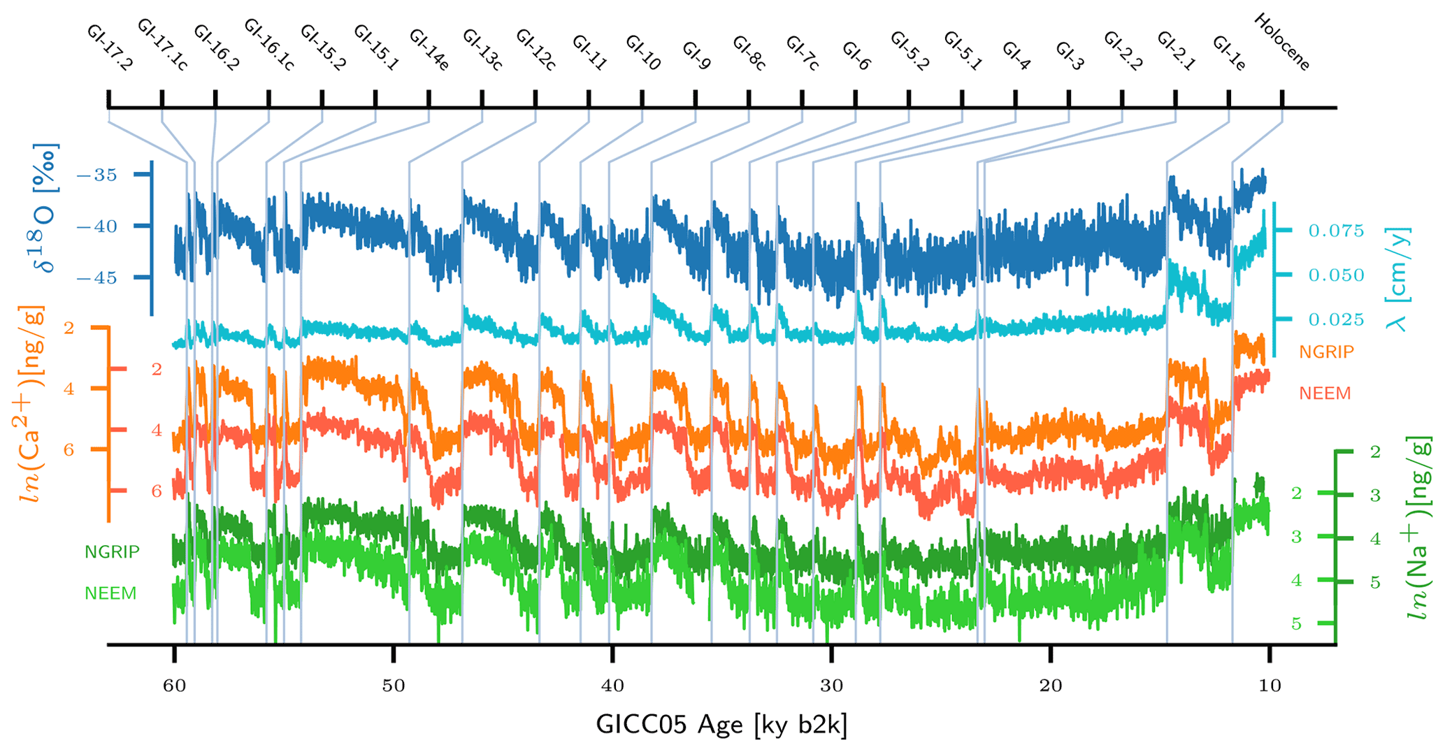
Figure 1Time series of δ18O (blue), annual layer thickness λ (cyan), Ca2+ (orange), and Na+ (green) from the NGRIP ice core, together with time series of Ca2+ (red) and Na+ (light green) from the NEEM ice core on the GICC05 timescale in ky b2k, at 10-year resolution. Light blue vertical lines mark the timings of major DO events. All time series are retrieved from Erhardt et al. (2019), and for the DO event timings and Greenland interstadial (GI) notation we followed Rasmussen et al. (2014). Originally, the δ18O record was published by NGRIP project members (2004) as 50-year mean values and later at higher resolution (5 cm) as a Supplement to Gkinis et al. (2014). The GICC05 age scale for the NGRIP ice core was compiled by Vinther et al. (2006), Rasmussen et al. (2006), Andersen et al. (2006), and Svensson et al. (2008). For the NEEM ice core, the GICC05 presented by Rasmussen et al. (2013) is used here.
Apart from δ18O, other Greenland ice core proxy records, such as Ca2+ and Na+ concentrations as well as the annual layer thickness λ, also bear the signature of DO cycles, as can be seen in Fig. 1 (e.g., Erhardt et al., 2019; Fuhrer et al., 1999; Ruth et al., 2007). While δ18O is interpreted as a qualitative proxy for ice core site temperatures (e.g. Gkinis et al., 2014; Jouzel et al., 1997; Johnsen et al., 2001), changes in Ca2+ concentrations – or equivalently dust – are believed to reflect changes in the atmospheric circulation (Ruth et al., 2007; Erhardt et al., 2019). Na+ concentration records indicate past sea-salt aerosol concentrations and are thought to negatively correlate with North Atlantic sea-ice cover (Erhardt et al., 2019; Schüpbach et al., 2018). The annual layer thickness depends on past accumulation rates at the drilling site and hence indicates local precipitation driven by synoptic circulation patterns (Erhardt et al., 2019). According to this proxy record interpretation, DO events comprise not only sudden warming but also a sudden increase in local precipitation amounts, retreat of the North Atlantic sea-ice cover, and changes in hemispheric circulation patterns.
In the search for the mechanism(s) causing or triggering DO events, several attempts have been made to deduce the relative temporal order of these abrupt changes by analyzing the phasing of corresponding abrupt shifts detected in multi-proxy time series from Greenland ice cores (Erhardt et al., 2019; Thomas et al., 2009; Steffensen et al., 2008; Ruth et al., 2007). While Thomas et al. (2009) and Steffensen et al. (2008) report delayed Greenland warming with respect to atmospheric changes for the onsets of GI-8 and GI-1 and the Holocene, Ruth et al. (2007) find no systematic lead or lag across the onsets of GI-1 to GI-24. However, the comprehensive study conducted by Erhardt et al. (2019) concludes that, on average, initial changes in both terrestrial dust aerosol concentrations (Ca2+) and local precipitation (λ) have preceded the changes in local temperatures (δ18O) and sea-salt aerosol concentrations (Na+) by roughly 1 decade at the onset of DO events during the last glacial cycle.
These observation-based studies are complemented by numerous conceptual theories and modeling studies that explore a variety of mechanisms to explain the DO events. Many studies emphasize the role of the AMOC in the emergence of DO events (Broecker et al., 1985; Clark et al., 2002; Ganopolski and Rahmstorf, 2001; Henry et al., 2016). In this context, Vettoretti and Peltier (2018) identified a self-sustained sea-salt oscillation mechanism to initiate transitions between stadials and interstadials in a comprehensive general circulation model (GCM) run, while Boers et al. (2018) proposed a coupling between sea-ice growth, subsurface warming, and AMOC changes to explain the DO cycles. Moreover, Li and Born (2019) draw attention to the subpolar gyre, a sensitive region that features strong interactions between atmosphere, ocean, and sea ice. In line with the empirical studies that suggest a delayed Greenland warming with respect to atmospheric changes, Kleppin et al. (2015) and Zhang et al. (2014) find DO-like transitions in GCM studies triggered by an abrupt reorganization of atmospheric circulation patterns.
Here, we refine the investigation of a potential pairwise lead–lag relationship between the four climate proxies Ca2+, Na+, δ18O, and the annual layer thickness λ at DO transition onsets, as previously presented by Erhardt et al. (2019), by rigorously taking into account the uncertainties of the DO onset detection in the different proxy records. We use the same data and the same probabilistic transition onset detection method as provided by Erhardt et al. (2019). The data comprise piecewise high-resolution (7 years or higher) multi-proxy time series around 23 major DO events from the later half of the last glacial cycle, from the NEEM and the NGRIP ice cores (Erhardt et al., 2019). The fact that high-frequency internal climate variability blurs abrupt transitions limits the ability to precisely detect their onset in the proxy data and thereby constitutes the main obstacle for the statistical analysis of the succession of events. The method designed by Erhardt et al. (2019) very conveniently takes this into account and instead of returning scalar estimators it quantifies the transition onsets in terms of Bayesian posterior probability densities that indicate the plausibility of a transition onset at a certain time in view of the data. This gives rise to a set of uncertain DO transition onset lags for each pair of proxies under study, whose statistical interpretation is the goal of this study.
While Erhardt et al. (2019) report transition onsets, midpoints, and endpoints, we restrict our investigation to the transition onset points, since we consider the leads and lags between the initial changes in the different proxy records to be the relevant quantity for a potential identification of the physical trigger of the DO events. We extend the previous work by interpreting the sets of uncertain lags as samples generated in random experiments from corresponding unknown populations – each proxy pair is associated with its own population of lags. This allows for the investigation of whether the reported average lags (Erhardt et al., 2019) are a systematic feature or whether they might have emerged by chance. In order to review the statistical evidence for potential systematic lags, we formalize the notion of a “systematic lag”: we call a lag systematic if it is enshrined in the random experiment in form of a population mean different from 0. Samples generated from such a population with a non-zero mean would systematically (and not by chance) exhibit sample means different from 0. Accordingly, we formulate the null hypothesis that the proposed transition sequence is in fact not physically favored. In mathematical terms this corresponds to an underlying population of lags with a mean equal to 0 or with reversed sign with respect to the observed lags. A rejection of this null hypothesis would statistically corroborate the interpretation that transitions in δ18O and Na+ systematically lag their counterparts in λ and Ca2+. On the other hand, acceptance of the hypothesis would prevent us from ruling out that the observed lag tendencies are a coincidence and not a systematic feature. We have identified three different statistical tests suitable for this task, which all rely on slightly different assumptions. Therefore, in combination they yield a robust assessment of the observations. Most importantly, we propagate the uncertainties that arise from the transition onset detection to the level of p values of the different tests.
We will show that, if the uncertainties are averaged out at the level of the individual transition onset lags – thus ignoring the uncertainties in the onset detection – all tests indicate statistical significance (at 5 % confidence level) of the observed tendencies toward delayed δ18O and Na+ transition onsets with respect to the corresponding onsets in λ and Ca2+. Rigorous uncertainty propagation, however, yields substantial probabilities for the observed transition onset lags to be non-significant with respect to the null hypothesis. We thus argue that the uncertainties in the transition onset detection are too large to infer a population mean different from 0 in the direction of the observed tendencies. In turn, this prevents the attribution of the observed lead–lag relations to a fundamental mechanism underlying the DO events. We discuss the difference between our approach and the one followed by Erhardt et al. (2019) in detail below.
In addition to the quantitative uncertainty discussed here, there is always qualitative uncertainty about the interpretation of climate proxies. Clearly, there is no one-to-one mapping between proxy variables and the climate variables they are assumed to represent. To give an example, changes in the atmospheric circulation will simultaneously impact the transport efficiency of sea-salt aerosols to Greenland. Schüpbach et al. (2018) discuss in detail the entanglement of transport efficiency changes and source emission changes for aerosol proxies measured in Greenland ice cores. We restrict our analysis to those proxy pairs that have been found to show decadal-scale time lags by Erhardt et al. (2019) and leave aside those pairs which show almost simultaneous transition onsets according to Erhardt et al. (2019).
This article is structured as follows: first, the data used for the study are described. Second, we introduce our methodology in general terms, in order to facilitate potential adaptation to structurally similar problems. Within this section, we pay special attention to clarifying the differences between the approaches chosen in this study and by Erhardt et al. (2019). This is followed by the presentation of our results including a comparison to previous results. In the subsequent discussion, we give a statistical interpretation and explain how the two lines of inference lead to different conclusions. The last section summarizes the key conclusions that can be drawn from our analysis.
In conjunction with their study, Erhardt et al. (2019) published 23 highly resolved time series for Ca2+ and Na+ concentrations from the NGRIP and NEEM ice cores for time intervals of 250 to 500 years centered around DO events from the later half of the last glacial. The data set covers all major interstadial onsets from GI-17.2 to the Holocene, as determined by Rasmussen et al. (2014). The time resolution decreases from 2 to 4 years with increasing depth in the ice cores due to the thinning of the core. In addition, Erhardt et al. (2019) derived the annual layer thickness from the NGRIP aerosol data and published these records likewise for the time intervals described above. Furthermore, continuous 10-year resolution versions of the proxy records were published, which cover the period 60–10 kyr BP, shown in Fig. 1 (Erhardt et al., 2019). Finally, the NGRIP δ18O record at 5 cm resolution (corresponding to 4–7 years for the respective time windows) (North Greenland Ice Core Project members, 2004) completes the data set used in the study by Erhardt et al. (2019) and correspondingly in our study.
While Ca2+ and Na+ mass concentrations are interpreted as indicators of the past state of the atmospheric large-scale circulation and the past North Atlantic sea-ice extent, respectively, the annual layer thickness and δ18O records give qualitative measures of the local precipitation and temperature, respectively (Erhardt et al., 2019, and references therein). The high resolution and the shared origin of the time series make them ideally suited to study the succession of events at the beginning of DO transitions. On top of that, the aerosol data have been co-registered in a continuous flow analysis allowing for the highest possible comparability (Erhardt et al., 2019).
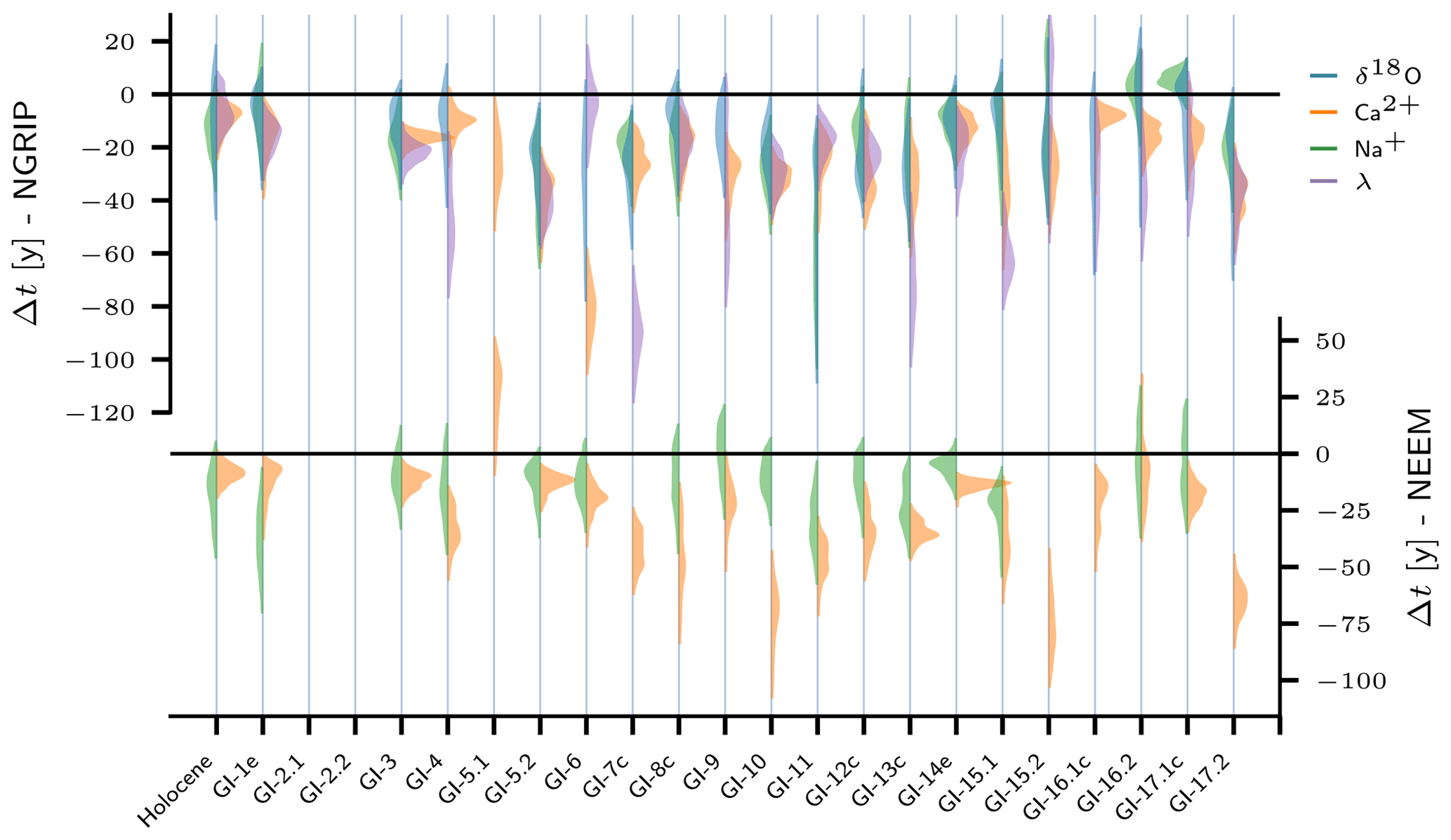
Figure 2DO events (Greenland interstadial onsets) for which Erhardt et al. (2019) provide high-resolution proxy data (, and λ) for windows centered around the transitions. δ18O data for the corresponding windows were retrieved from continuous δ18O time series measured in 5 cm steps in the NGRIP ice core (see Fig. 1). The posterior probability densities for the transition onsets with respect to the timing of the DO events according to Rasmussen et al. (2014) are shown in arbitrary units for all proxies. They were recalculated using the data and the method provided by Erhardt et al. (2019). The uncertain transition onsets are only shown for those transitions investigated in this study – the selection is adopted from Erhardt et al. (2019) to guarantee comparability.
For their analysis, Erhardt et al. (2019) only considered time series around DO events that do not suffer from substantial data gaps. For the sake of comparability, we adopt their selection. From Fig. 2 it can be inferred which proxy records around which DO events have been included in this study. For details on the data and the proxy interpretations we refer to Erhardt et al. (2019) and the manifold references therein.
We first briefly review the probabilistic method that we adopted from Erhardt et al. (2019) in order to estimate the transition onset time t0 of each proxy variable for each DO event comprised in the data (see Fig. 3). The Bayesian method accounts for the uncertainty inherent to the determination of t0 by returning probability densities instead of scalar estimators. From these distributions, corresponding probability distributions for the pairwise time lags between two proxies can be derived for all DO events. Second, a statistical perspective on the series of DO events is established. For a given proxy pair, the set of transition onset lags from the different DO events is treated as a sample of observations from an unknown underlying population. In this very common setup, naturally one would use hypothesis tests to constrain the population. In particular, the question of whether any lag tendencies observed in the data are a systematic feature or whether they have instead occurred by chance can be assessed by testing a convenient null hypothesis. However, the particularity that the individual observations that comprise the sample are themselves subject to uncertainty requires a generalization of the hypothesis tests. We propagate the uncertainty of the transition onset timings to the p values of the tests and hence obtain uncertain p values in terms of probability densities (see Figs. 4 and 7). While in common hypothesis tests the scalar p value is compared to a predefined significance level, here we propose two criteria to project the p-value distribution onto the binary decision between acceptance and rejection of the null hypothesis. After this general characterization of the statistical problem, we introduce the tests which we employ for the analysis. Finally, we compare our approach to the one followed by Erhardt et al. (2019).
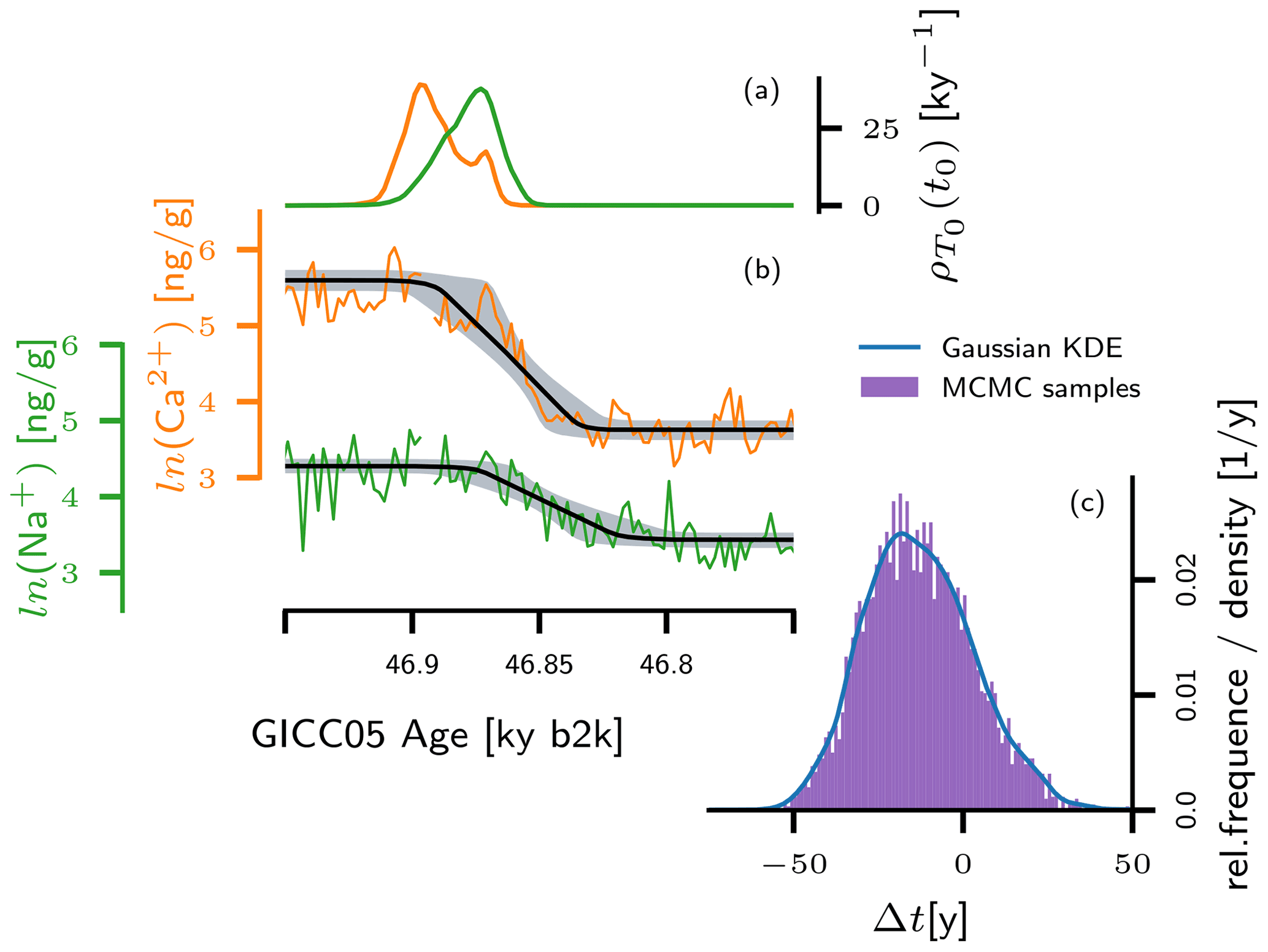
Figure 3(a) Posterior probability distribution for the onset of NGRIP Ca2+ and Na+ transitions associated with the onset of GI-12c, derived from Ca2+ (orange) and Na+ (green) values around the GI-12c onset at 2-year resolution, using the probabilistic ramp-fitting shown in (b). The black lines in (b) indicate the expected ramp, i.e., the average over all ramps determined by the posterior distributions of the ramp parameters. The grey shaded area indicates the 5th–95th percentiles of these ramps. (c) Histogram sampled from the posterior distribution for the transition onset lag Δt between the two proxies (violet), together with the corresponding Gaussian kernel density estimate (KDE, blue).
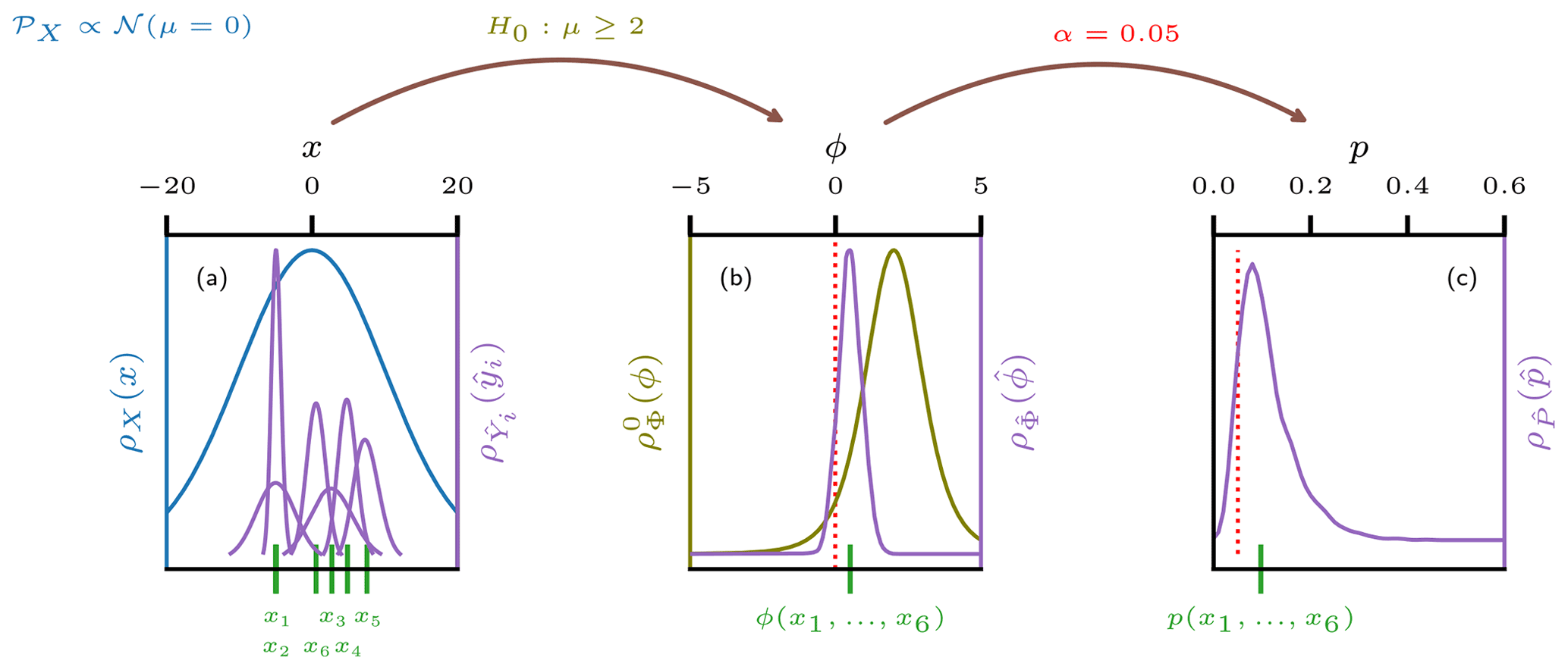
Figure 4(a) Schematic representation of an uncertain observation of a sample (purple) generated from a population (blue) in a random experiment. The blue line indicates the probability density of the generating population 𝒫X. Green lines indicate the true value of a sample realized from 𝒫X. If the observational process involves uncertainty, a second level of randomness is introduced and the values can at best be approximated by probability density functions depicted in purple. These uncertainty distributions indicate the informed estimate of the observer about how likely a certain value for the estimator is to coincide with the true value xi. Depending on the measurement process, the uncertainty distributions of the sample members may all exhibit individual shapes or they may share a common one. (b) Distribution of the uncertain test statistic derived from the uncertain sample (purple) together with the corresponding value derived from the true sample (green). In olive, the distribution of Φ under the null hypothesis is shown. The dotted red line separates the rejection region (left) from the acceptance region in a one-sided test setup. (c) Distribution of the uncertain p value corresponding to the uncertain sample. In green, the p value of the certain sample is marked. The red line indicates the significance level α.
3.1 Transition onset detection
Consider a fluctuating time series with n data points, which includes one abrupt transition from one level of values to another, as shown in Fig. 3b. For this setting, Erhardt et al. (2019) have designed a method to estimate the transition onset time t0 in a probabilistic, Bayesian sense. The application of the method to NGRIP Ca2+ and Na+ concentration data around the onset of GI-12c is illustrated in Fig. 3. Instead of a point estimate, their method returns a so-called posterior probability density that indicates the plausibility of the respective onset time in view of the data (see Fig. 3a). For technical reasons, this probability density cannot be derived in form of a continuous function but only in form of a representative set of values generated from it by means of a Markov chain Monte Carlo (MCMC) algorithm (Goodman and Weare, 2010).
The key idea is to model the transition as a linear ramp ℒ(ti) perturbed by red noise ϵ(ti), which is an autoregressive process of first order:
This model is fully determined by the four ramp parameters , the amplitude σ, and the autoregressive coefficient α of the AR(1) process. For a given configuration θ of these six parameters, the probability of this stochastic model to exactly reproduce the data 𝒟 reads
where denotes the residuals between the linear ramp and the observations and δ0=0. Bayes' theorem immediately yields the posterior probability density for the model parameters π(θ|𝒟) upon introduction of convenient priors π(θ):
where the normalization constant is the a priori probability of the observations. Since the parameter space is six-dimensional, Eq. (3) cannot be evaluated explicitly on a grid with reasonably fine spacing. Instead, an MCMC algorithm is used to sample a representative set of parameter configurations from the posterior distribution that approximates the continuous distribution in the sense that for smooth functions f
where the notion of a so-called empirical distribution has been used. The use of the MCMC algorithm further allows us to omit the normalization constant π(𝒟). The number m of individuals comprised in the MCMC sample must be chosen large enough to ensure a good approximation in Eq. (4). The marginal distribution for the parameter t0 relevant for our study can be obtained by integration over the remaining parameters θ*:
which reads
in terms of the empirical density induced by the MCMC sample.
Given the probability densities for the transition onsets of two proxy variables p and q at a chosen DO event i, the probability density for the lag between them reads
was chosen to denote the time lag which inherits the uncertainty from the transition onset detection and must thus mathematically be treated as a random variable. denotes a potential value that may assume. The set of probability densities derived from the different DO events conveniently describes the random vector of uncertain DO onset lag observations for the (p,q) proxy pair in the sense that
Note that the entries of the random vector ΔTp,q are independent from each other and follow their individual distributions , such that the joint distribution is given by the product of the individual distributions. A cross-core comparison is not possible because the relative dating uncertainties between the cores exceed the magnitude of the potential time lags.
For the sake of simplicity, we omit the difference between the posterior density distribution and the empirical posterior density distribution induced by an MCMC sample. It is shown in Appendix A that all methods can be equivalently formulated in terms of the empirical posterior density distribution. The numerical computations themselves have of course been carried out with the empirical densities obtained from the MCMC sampler. Appendix B discusses the construction of numerically manageable empirical densities . Since a substantial reduction in the available MCMC sampled data is required, a control group of alternative realizations of is introduced. The high agreement of the results obtained from the control group with the results discussed in the main text confirms the validity of the initial construction.
In the following, all probability densities that represent uncertainties with origin in the transition onset observation will be referred to as uncertainty distributions or uncertainty densities. This helps to distinguish them from probability distributions that generically characterize random experiments. The random variables described by uncertainty distributions will be termed uncertain variables and will be marked with a hat. Generally, we denote all random (uncertain) variables by capital letters X (), while realizations will be denoted with lower-case letters x (). Furthermore, distributions will always be subscripted with the random variables that they characterize, e.g., ρX(x) (). For the sake of readability, sometimes we omit the index p,q when it is clear that a quantity refers to a pair of proxies (p,q).
3.2 Statistical setting
Despite their diversity in terms of temperature amplitude, duration, and frequency across the last glacial, the reoccurring patterns and their common manifestation in different proxies suggest that the DO events follow a common physical mechanism. If this assumption holds true, this mechanism prescribes a fixed pattern of causes and effects for all DO events – at least on the scale of interactions between climatic subsystems represented by the proxies under study. However, natural variability randomly delays or advances the individual parts of the event chain of the DO mechanism in each single realization, without violating the mechanistic causality. The observed pairwise transition onset lags can thus be regarded as realizations of independent and identically distributed (i.i.d.) random variables generated in a random experiment on the sample space Ω=ℝ. Here, ℱ is a σ algebra defined on Ω and may be taken as the Borel algebra. – the so-called population – denotes a probability measure with respect to ℱ and fully characterizes the random lag ΔTp,q between the proxies p and q. Importantly, if any of the proxy variables investigated here was to represent a climate variable associated with the DO event trigger, we would expect an advanced initial change in the record of this proxy with respect to other proxies at DO events. In turn, a pronounced delay of a proxy record's transition onset contradicts the assumption that the proxy represents a climate variable associated with the trigger. Therefore, the identification of leads and lags between the transition onsets in the individual proxy time series may help in the search for the trigger of the DO events. Here, we formalize the investigation of systematic lead–lag relationships between the proxy transitions. The random experiment framework allows us to relate a suspected transition sequence to a mean of the generating population differing from 0 in the according direction. Evidence for the suspected sequence can then be obtained by testing the null hypothesis of a population mean equal to 0 or with a sign opposed to the suspected lag direction. If this null hypothesis can be rejected based on the observations, this would constitute a strong indication of a systematic, physical lag and would hence potentially yield valuable information on the search for the mechanism(s) and trigger(s) of the DO transitions.
According to the data selection by Erhardt et al. (2019) as explained in Sect. 2, for all studied pairs of proxies we compute either 16 or 20 transition lags from the different DO events, which we interpret as samples from their respective populations . Studying these samples, Erhardt et al. (2019) deduced a decadal-scale delay in the transition onsets in Na+ and δ18O records with respect to their counterparts in Ca2+ and λ. In order to test if the data support evidence for this lag to be systematic in a statistical sense, the notion of a “systematic lag” first needs to be formalized mathematically. We argue that a physical process that systematically delays one of the proxy variable transitions with respect to another must in the random experiment framework be associated with a population that exhibits a mean different from 0: . The outcomes of such a random experiment will systematically exhibit sample means different from 0 in accordance with the population mean. Samples generated from a population with a mean equal to 0 may as well yield sample means that strongly differ from 0. However, their occurrence is not systematic but rather a coincidence. Given a limited number of observations, hypothesis tests provide a consistent yet not unambiguous way to distinguish systematic from random features. If the mean of the observed sample indicates an apparent lag between the proxies p and q, testing whether the sample statistically contradicts a population that favors no () or the opposite lag (or ) can provide evidence at the significance level α for the observed mean lag to be systematic in the sense that . However, as long as the null hypothesis cannot be rejected, the observed average sample lag cannot be regarded as statistical evidence for a systematic lag.
Before we introduce the tests deployed for this study, we discuss the particularity that the individual observations of the i.i.d. variables that comprise our samples are themselves subject to uncertainty and hence are represented by probability densities instead of scalar values. The common literature on hypothesis tests assumes that an observation of a random variable yields a scalar value. Given a sample of n scalar observations
the application of hypothesis tests to the sample is in general straight forward and has been abundantly discussed (e.g. Lehmann and Romano, 2006). In short, a test statistic ϕx=ϕ(x) is computed from the observed sample, where
denotes the mapping from the space of n-dimensional samples to the space of the test statistic and ϕx denotes the explicit value of the function when applied to the observed sample x. Subsequently, integration of the so-called null distribution over all values ϕ′, which under the null hypothesis H0 are more extreme than the observed ϕx, yields the test's p value. In this study, a hypothesis on the lower limit of a parameter will be tested. In this one-sided left-tailed application of hypothesis testing, the p value explicitly reads
which defines the mapping
Analogous expressions may be given for one-sided right-tailed and two-sided tests. The null distribution is the theoretical distribution of the random test statistic Φ=ϕ(X) under the assumption that the null hypothesis on the population 𝒫X holds true. If px is less than a predefined significance level α, the observed sample x is said to contradict the null hypothesis at the significance level α, and the null hypothesis should be rejected.
In contrast to this setting, the DO transition onset lags between the proxies p and q, which are thought to have been generated from the population , are observed with uncertainty. In our case, the entries in the vector of observations are uncertain variables themselves, which are characterized by the previously introduced uncertainty distributions . Figure 4a illustrates this situation: from an underlying population 𝒫X a sample is realized, with xi denoting the true values of the individual realizations. However, the exact value of xi cannot be measured precisely due to measurement uncertainties. Instead, an estimator is introduced together with the uncertainty distribution that expresses the observer's belief about how likely a specific value for the estimator is to agree with the true value xi. The correspond to the . For the xi there is no direct correspondence in the problem at hand because this quantity cannot be accessed in practice and is thus not denoted explicitly. We call the vector of estimators an uncertain sample in the following. Omitting the (p,q) notation, we denote an uncertain sample of time lags as
with
Note that the uncertainty represented by the uncertain sample originates from the observation process – the sample no longer carries the generic randomness of the population 𝒫ΔT it was generated from. The are no longer identically but yet independently distributed.
A simplistic approach to test hypotheses on an uncertain sample would be to average over the uncertainty distribution and subsequently apply the test to the resulting expected sample
Averaging out uncertainties, however, essentially implies that the uncertainties are ignored and is thus always associated with a loss of information. The need for a more thorough treatment, with proper propagation of the uncertainties, may be illustrated by a simple consideration. Assume that a random variable X can be observed at a given precision σobs, where σobs may be interpreted as the typical width of the corresponding uncertainty distribution. For any finite number of observations of X, the measurement uncertainty limits the ability to infer properties of the population. For example, one cannot distinguish between potential candidates μ0 and μ1 for the population mean, whose difference is a lot smaller than the observational precision, unless the number of observations tends to infinity. If uncertainties are averaged out, testing against the alternative can eventually still yield significance, even in the case where . For relatively small sample sizes, such an attested significance would be statistically meaningless. The uncertainties in the individual measurements considered here are on the order of a few decades, while the proposed size of the investigated time lag is roughly 1 decade. In combination with the relatively small sample sizes of either 16 or 20 events, the scales involved in the analysis require a suitable treatment of the measurement uncertainties.
The uncertainty propagation relies on the fact that applying a function to a real valued random (uncertain) variable X yields a new random (uncertain) variable G=f(X), which is distributed according to
Analogously, the uncertain test statistic follows the distribution
Repeated application of Eq. (15) yields the uncertainty distribution of a given test's p value :
In the example shown in Fig. 4 the initial uncertainties in the observations translate into an uncertain p value that features both probability for significance and probability for non-significance. This illustrates the need for a criterion to project the uncertain p value onto a binary decision space comprised of rejection and acceptance of the null hypothesis. We propose to consider the following criteria to facilitate an informed decision:
-
The hypothesis shall be rejected at the significance level α if and only if the expected p value is less than α, that is
-
The hypothesis shall be rejected at the significance level α if and only if the probability of p to be less than α is greater than a predefined threshold η (we propose η=90 %), that is
While the p value of a certain sample indicates its extremeness with respect to the null distribution, the expected p value may be regarded as a measure of the uncertain sample's extremeness. Given the measurement uncertainty, the quantity constitutes an informed assessment of how likely or plausible the true value of the measured sample is to be statistically significant with respect to the null hypothesis. Thus, the first criterion assesses how “strongly” the uncertain sample contradicts the null hypothesis, while the second criterion evaluates the likelihood of the uncertain sample to contradict the null hypothesis. The choice of η is arbitrary and may be tailored to the specific circumstances of the test. In some situations, one might want to reject the null hypothesis only in the case of a high probability of significance and therefore choose a large value for η – e.g., when mistakenly attested significance is associated with high costs. In other situations, even small probabilities for significance may be important, e.g., if a significant test result would be associated with high costs or with high risks. We propose to assess the two criteria in combination. In the case of them not yielding the same result, the weighing between the criteria must be adapted to the statistical problem at hand.
3.3 Hypothesis tests
We have introduced the notion of uncertain samples and its consequences for the application of hypothesis tests. Here, we briefly introduce the tests used to test our null hypothesis that the observed tendency for delayed transition onsets in Na+ and δ18O with respect to Ca2+ and λ has occurred by chance and that the corresponding populations that characterize the pairwise random lags ΔTp,q in fact do not favor the tentative transition orders apparent from the observations. Mathematically, this can be formulated as follows:
-
Let be the probability density associated with the population of DO transition onset lags between the proxy variables p and q and let the observations suggest a delayed transition of the proxy q – that is, the corresponding uncertainty distributions indicate high probabilities for negative across the sample according to Eq. (7). We then test the hypothesis H0: The mean value of the population is greater than or equal to zero.
We identified three tests that are suited for this task, namely the t test, the Wilcoxon signed-rank (WSR) test, and a bootstrap test. The WSR and the t test are typically formulated in terms of paired observation {xi,yi} that give rise to a sample of differences which correspond to the time lags of different DO events (Rice, 2007; Lehmann and Romano, 2006, e.g.). The null distributions of the tests rely on slightly different assumptions regarding the populations. Since we cannot guarantee the compliance of these assumptions, we apply the tests in combination to obtain a robust assessment.
3.3.1 t test
The t test (Student, 1908) relies on the assumption that the population of differences 𝒫D is normally distributed with mean μ and standard deviation σ. For a random sample the test statistic
follows a t distribution tn−1(z) with n−1 degrees of freedom. Here, is the sample mean and is the samples' standard deviation. This allows us to test whether an observed sample contradicts a hypothesis on the mean μ. To compute the p value for the hypothesis (left-handed application) the null distribution is integrated from −∞ to the observed value z(d):
The resulting p value must then be compared to the predefined significance level α.
The t test can be generalized for application to an uncertain sample of the form as follows: let denote the uncertainty distribution of . Then according to Eq. (15) the distribution of the uncertain statistic reads
Finally, the distribution of the uncertain p value may again be computed according to Eq. (15)
and then be evaluated according to the two criteria formulated above.
3.3.2 Wilcoxon signed rank
Compared to the t test, the WSR test (Wilcoxon, 1945) allows us to relax the assumption of normality imposed on the generating population 𝒫D and replaces it by the weaker assumption of symmetry with respect to its mean μ in order to test the null hypothesis . The test statistic W for this test is defined as
where denotes the rank of within the sorted set of the absolute values of differences . The Heaviside function Θ(Di) guarantees that exclusively Di>0 values are summed. The derivation of the null distribution is a purely combinatorial problem and its explicit form can be found in lookup tables. Because we denote the null distribution by to signal that this is not a continuous density. Explicitly, the null distribution can be derived as follows: first, the assumption of symmetry around 0 (for the hypothesis , the relevant null distribution builds on μ=0) guarantees that the chance for Di to be positive is equal to . Hence, the number of positive outcomes m follows a symmetric binomial distribution . For m positive observations, there are different sets of ranks that they may assume and which are again, due to the symmetry of 𝒫D, equally likely. Hence, for a given number of positive outcomes m the probability to obtain a test statistic w is given by the share of those configurations that yield a rank sum equal to w. Summing these probabilities over all possible values of m yields the null distribution for the test statistic w.
For a given sample d we test the hypothesis by computing the corresponding one-sided p value pw, which is given by the cumulative probability that the null distribution assigns to w′ values smaller than the observed w(d):
Since it follows that Pw assumes only discrete values in [0,1] with the null distribution determining the mapping between these two sets.
The generalization of the WSR test to the uncertain sample can be carried out almost analogously to the t test. However, the fact that makes it inconvenient to use a continuous probability density distribution. We denote the distribution for the uncertain by
Given the one-to-one map from all to the set of discrete potential values pw for Pw in [0,1] determined by Eq. (25), the probability to obtain is already given by the probability to obtain the corresponding . Hence, we find
3.3.3 Bootstrap test
Given an observed sample of differences , a bootstrap test constitutes a third option to test the compatibility of the sample with the hypothesis that the population of differences features a mean equal to or greater than 0: . Guidance for the construction of a bootstrap hypothesis test can be found in Lehmann and Romano (2006) and Hall and Wilson (1991). The advantage of the bootstrap test lies in its independence from assumptions regarding the distributions' shape. Lehmann and Romano (2006) propose the test statistic
with denoting the sample mean. In contrast to the above two tests, the bootstrap test constructs the null distribution directly from the observed data. In the absence of assumptions, the best available approximation of the population 𝒫D is given by the empirical density
However, the empirical density does not necessarily comply with the null hypothesis and it thus has to be shifted accordingly:
corresponds to the borderline case of the null hypothesis μ=0. The null distribution for v is then derived by resampling m synthetic samples of size n from and computing for each of them. This corresponds to randomly drawing n values from the set d−u with replacement and computing v for the resampled vectors m times, where the index j labels the iteration of this process. The resulting set induces the data-driven null distribution for the test statistic
Setting m=10 000 we obtain robust null distributions for the two cases relevant here (n=16 and n=20). The p value of this bootstrap test is then computed as before in a one-sided manner:
where the right-hand side equals the fraction of resampled that are smaller than v(d) of the original sample.
In the case where the sample of differences is uncertain, as for , the construction scheme for needs to be adjusted to reflect these uncertainties. In principle, each possible value for the uncertain is associated with its own null distribution . In this sense, the value for the test statistic should be compared to the corresponding to derive a p value for this . Equations (31) and (32) define a mapping from to its corresponding p value. To compute the uncertainty distribution for the p value, this map has to be evaluated for all potential , weighted by the uncertainty distribution :
The three tests are applied in combination in order to compensate for their individual deficits. If the population 𝒫ΔT was truly Gaussian, the t test would be the most powerful test; i.e., its rejection region would be the largest across all tests on the population mean (Lehmann and Romano, 2006). Since normality of 𝒫ΔT cannot be guaranteed, the less powerful Wilcoxon signed-rank test constitutes a meaningful supplement to the t test, relying on the somewhat weaker assumption that 𝒫ΔT is symmetric around 0. Finally, the bootstrap test is non-parametric and in view of its independence from any assumptions adds a valuable contribution.
3.4 Comparison to previous analysis
For the derivation of the transition lag uncertainty distributions of the ith DO event between the proxies p and q, we have directly adopted the methodology designed by Erhardt et al. (2019). However, our statistical interpretation of the resulting sets of uncertainty distributions derived from the set of DO events differs from the one proposed by Erhardt et al. (2019). In this section we explain the subtle yet important differences between the two statistical perspectives.
Given a pair of variables (p,q), Erhardt et al. (2019) define what they call “combined estimate” as the product over all corresponding lag uncertainty distributions:
This implicitly assumes that all DO events share the exact same time lag Δt* between the variables p and q. This is realized by inserting a single argument Δt* into the different distributions . Hence, the product on the right-hand side of Eq. (34) in fact indicates the probability that all DO events assume the time lag Δt*, provided that they all assume the same lag:
The denominator on the right-hand side equals the probability that all DO events share a common time lag. Equation (34) strongly emphasizes those regions where all uncertainty distributions are simultaneously substantially larger than 0. The combined estimate answers the question: provided that all DO events exhibit the same lag between the transition onsets of p and q, then how likely is it that this lag is given by Δt*. Drawing on this quantity, Erhardt et al. (2019) conclude that δ18O and Na+ “on average” lag Ca2+ and λ by about 1 decade.
Thinking of the DO transition onset lags as i.i.d. random variables of a repeatedly executed random experiment takes into account the natural variability between different DO events, and hence it removes the restricting a priori assumption . In our approach we have related the potentially systematic character of lags to the population mean. Since the sample mean is the best point estimate of a population mean, we consider it to reasonably indicate potential leads and lags, whose significance should be tested in a second step. Thus, we ascribe to the sample mean a similar role as Erhardt et al. (2019) ascribe to the combined estimate, and therefore we present a comparison of these two quantities in Sect. 4.1.
The mean of an uncertain sample is again an uncertain quantity and its distribution reads
While the combined estimate multiplies the distributions , the uncertain sample mean convolutes them pairwise (see Appendix C). We thus expect the distributions for uncertain sample means to be broader than the corresponding distributions for the combined estimate. This can be motivated by considering the simple example of two Gaussian variables X and Y. According to the convolution their sample mean is normally distributed with variance . In contrast, a combined estimate would yield a normal distribution with variance . Thus, the convolution will appear broader for all , which is the case for the distributions considered in this study.
In the following we apply the above methodology to the different pairs of proxies that Erhardt et al. (2019) found to exhibit a decadal-scale time lag, based on an assessment of the combined estimate, namely , , , and (λ,δ18O) from the NGRIP ice core and from the NEEM ice core. For each individual proxy we estimate the uncertain transition onsets relative to the timing of the DO events as given by Rasmussen et al. (2014) (see Fig. 2). From these uncertain transition onsets, the uncertainty distributions for the sets of uncertain lags between the proxies p and q are derived according to Eq. (7). As mentioned previously, we study the same selection of transitions evidenced in the multi-proxy records as Erhardt et al. (2019). This selection yields sample sizes of either 16 or 20 lags per pair of proxies but not 23, which is the total number of DO events present in the data.
We first study the uncertain sample means. As already mentioned, the sample mean is the best available point estimate for the population mean. Hence, sample means different from 0 may be regarded as first indications for potential systematic lead–lag relationships and thus motivate the application of hypothesis tests. We compare the results obtained for the uncertain sample means with corresponding results for the combined estimate. Both quantities indicate a tendency towards a delayed transition in Na+ and δ18O. Accordingly, in the subsequent section we apply the generalized hypothesis tests introduced above to the uncertain samples of transition lags to test the null hypothesis that pairwise, the apparent transition sequence is not systematically favored, that is, that the populations have mean equal to or greater than 0.
4.1 Uncertain sample mean and combined estimate
Based on their assessment of the combined estimate, Erhardt et al. (2019) concluded that on average, transitions in Ca2+ and λ started approximately 1 decade earlier than their counterparts in Na+ and δ18O. Figure 5 shows a reproduction of their results together with the uncertainty distributions of the sample means for all proxy pairs under study ( and (λ,δ18O) are not shown in Erhardt et al., 2019). For an uncertain sample of lags between the proxies p and q, the combined estimate and the uncertain sample mean are computed according to Eqs. (35) and (36), respectively. The reproduction of the combined estimate deviates from the original publication by no more than 1 year with respect to the mean and the 5th and 95th percentiles across all pairs. These deviations might originate from the stochastic MCMC-sampling process used for the analysis.
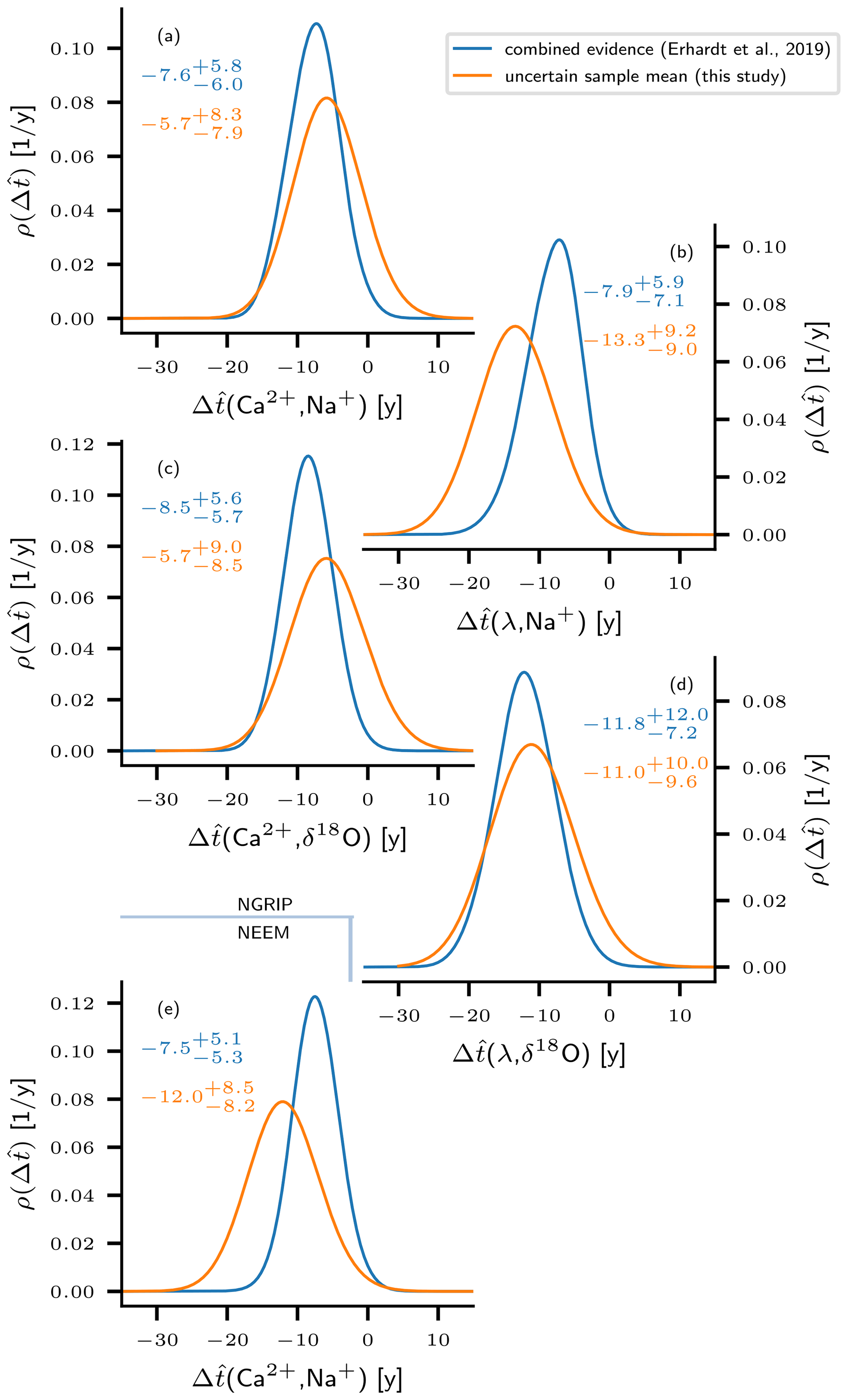
Figure 5Comparison between the uncertain sample means (this study) and “combined estimates” according to Erhardt et al. (2019). The probability densities for the combined estimate are derived from the samples of uncertain time lags according to Eq. (34). Correspondingly, the uncertain sample means are computed according to Eq. (36). The numbers in the plots indicate the mean, the 5th, and the 95th percentile of the respective quantity. Both computations use Gaussian kernel density estimates of the MCMC-sampled transition onsets lags. Panels (a–d) refer to proxy pairs from the NGRIP ice core, and panel (e) shows results from the NEEM ice core. The distributions for both the combined estimate and the uncertain sample mean point towards a delayed transition onset in δ18O and Na+ with respect to λ and Ca2+.
With the sample mean being the best point estimator of the population mean, it serves as a suitable indicator for a potential population mean different from 0. The expectations
for the sample means of all proxy pairs do in fact suggest a tendency towards negative values in all distributions, i.e., a delay of the Na+ and δ18O transition onsets with respect to Ca2+ and λ. This indication is weakest for () and () from NGRIP, since for these pairs we find a non-zero probability of a positive sample mean. For the other pairs the indication is comparably strong, with the 95th percentiles of the uncertainty distributions for the sample mean still being less than 0. Overall, the results for the uncertain mean confirm the previously reported tendencies, and in very rough terms, the distributions qualitatively agree with those for the combined estimate. In agreement with the heuristic example from Sect. 3.4, we find the sample mean distributions to be broader than the combined estimate distributions in all cases. The expected sample means indicate less pronounced lags for (Fig. 5a) and (Fig. 5c) from the NGRIP ice core compared to the expectations of the corresponding combined estimate. In combination with the broadening of the distribution, this yields considerable probabilities for U>0 of 12 % and 14 %, respectively, indicating a delayed transition of Ca2+ in the sample mean with respect to Na+ or δ18O. Contrarily, for (NGRIP, Fig. 5b) and (NEEM, Fig. 5e) the expected sample means point towards more distinct lags than reported by Erhardt et al. (2019) based on the combined estimate. For (λ,δ18O) (NGRIP, Fig. 5d) the sample mean and the combined estimate are very close. Note that the analysis of the uncertain sample values yields a more inconsistent picture with regard to the lag in the two different cores. While the distribution is shifted to less negative (less pronounced lag) for the NGRIP data, it tends to more negative values in the case of NEEM (stronger lag), suggesting a slight discrepancy between the cores.
Both quantities, the uncertain sample mean and the combined estimate point towards delayed transition onsets in Na+ and δ18O with respect to Ca2+ and λ, with major fractions of their uncertainty densities being allocated to negative values. This provides motivation to test whether the observations significantly contradict the hypothesis of a population mean equal to or greater than 0. Accordingly, the subsequent section presents the results obtained from the application of three different hypothesis tests that target the population mean. As discussed in Sect. 3, the tests have been modified to allow for a rigorous uncertainty propagation and return an uncertainty distribution for their corresponding p values rather than scalars.
4.2 Statistical significance of the proposed lead–lag relations
Above, we identified three tests for testing the hypothesis that the samples were actually generated from populations that on average feature no or even reversed time lags compared to what the sign of the corresponding uncertain sample mean suggests. Mathematically, this is equivalent to testing the hypothesis that the mean μp,q of the population is greater than or equal to 0: . A rejection of this hypothesis would confirm that the assessed sample is very unlikely to stem from a population with and would thereby provide evidence for a systematic lag. Under the constraints indicated above this would in turn yield evidence for an actual lead of the corresponding climatic process. We have chosen a significance level of α=0.05, which is a typical choice. Figure 7 summarizes the final uncertainty distributions of the three tests for all proxy pairs under study. Corresponding values are given in Table 1.
Table 1Results from the application of the t test, the WSR test, and a bootstrap test to uncertain samples of DO transition onset lags . denotes the expected p value, derived from the uncertainty-propagated p-value distribution. The probability of significant test results associated with the same distribution is indicated by . For comparison, the p values from the application of the tests to the expected sample are given in the bottom row.

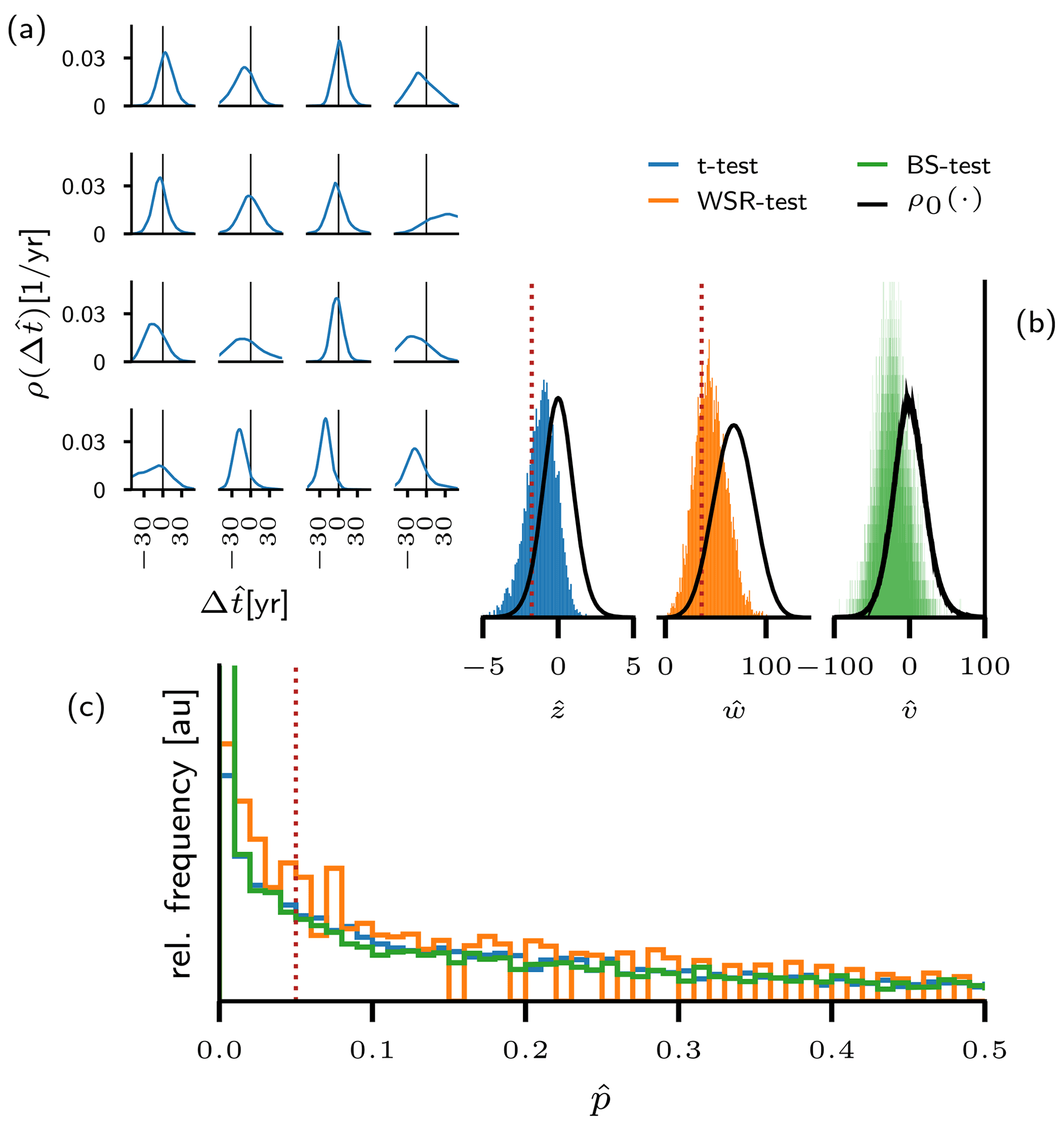
Figure 6Exemplary application of the analysis to the proxy pair from the NGRIP ice core. Panel (a) shows 16 uncertain time lags derived from the proxy data around DO events. The continuous densities have been obtained via a Gaussian kernel density estimate from the corresponding MCMC samples (see Sect. 3.1). In panel (b) the uncertain test statistics induced by the uncertain sample are shown for the t test (blue), the WSR test (orange), and a bootstrap test (green). The values that comprise the histograms are immediately derived from the MCMC samples. Panel (c) shows the empirical uncertainty distribution for the p values of the three tests, following from the uncertain test statistics in panel (b). Dotted red lines separate rejection from acceptance regions in panels (b) and (c). In the case of the bootstrap test, the rejection regions cannot be defined consistently on the level of the test statistic, since each possible value for the uncertain generates its individual null distribution. The null distribution shown here is in fact the pooled distribution of resampled obtained from all MCMC- sampled values for . For the other proxy pairs investigated in this study, corresponding plots would appear structurally similar.
Figure 6 exemplarily illustrates the application of the three tests to the empirical densities obtained for (NGRIP). In Fig. 6 the initial uncertainty in the observations – i.e., the uncertainty encoded by the distributions of transition onset lags – is propagated to an uncertain test statistic according to Eq. (16). In turn, the uncertain test statistic yields an uncertain p value (see Eq. 17). Since the numerical computation is based on empirical densities as generated by the MCMC sampling, we show the corresponding histograms instead of continuous densities – for , Gaussian kernel density estimates are presented only for the sake of visual clarity. On the level of the test statistics the red dashed line separates the acceptance from the rejection region, based on the null distributions given in black. Qualitatively, the three tests yield the same results. The histograms clearly indicate non-zero probabilities for the test statistic in both regions. Correspondingly, the histograms for the p values stretch well across the significance threshold. The shapes of the histograms resemble an exponential decay towards higher p values. This results from the non-linear mapping of the test statistics to the p values. Despite the pronounced bulk of empirical p values below the significance level, the probability of non-significant p values is still well above 50 % for the three tests (see Table 1). Also, the expected p value exceeds the significance level for all tests. Hence, neither of the two criteria for rejecting the null hypothesis formulated in Sect. 3.2 is met for the proxy pair . In contrast, if the observational uncertainties are averaged out on the level of the transition onset lags, all tests yield p values below the significance level, which would indicate that the lags were indeed significant. Hence, the rigorous propagation of uncertainties qualitatively changes the statistical assessment of the uncertain sample of lags (NGRIP). While the expected sample rejects the null hypothesis, rigorous uncertainty propagation leads to acceptance. This holds true for all tests.
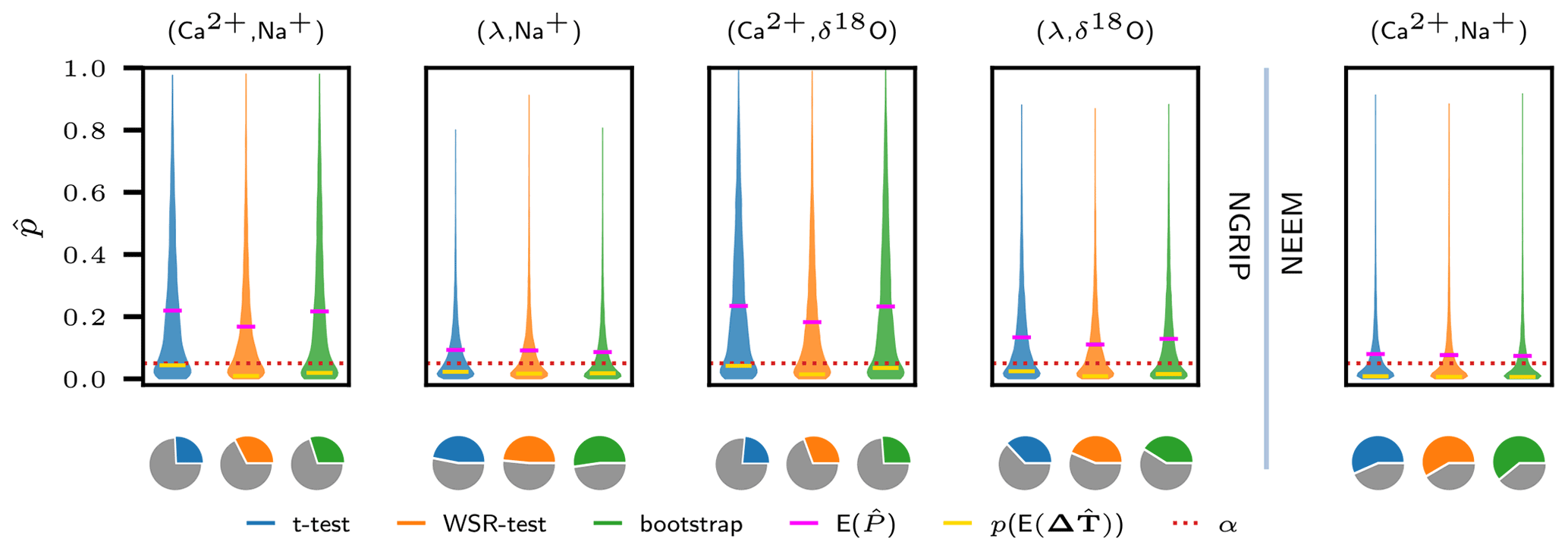
Figure 7Results of the hypothesis tests applied to the uncertain samples of transition onset lags . The violin plots show the Gaussian kernel density estimates of the empirical uncertainty distributions for p values (see Fig. 6) obtained for all tests and for all proxy pairs investigated. Pink bars indicate the corresponding expected p values and yellow bars indicate the p values obtained from testing the expected samples . All expected p values are above the significance level α=0.05 (red dotted line), while the expected samples appear to be significant consistently across all proxy pairs and all tests. The pie charts indicate the probability of the respective p values to be less then α.
Figure 7 summarizes the results obtained for all proxy pairs under study. Qualitatively, our findings are the same for the other pairs as for the (NGRIP) case discussed in detailed above. All expected p values, as indicated by the pink bars, are above the significance level. Also, the probability for significance is below 60 % for all pairs and all tests as shown by the pie charts. Therefore, for all proxy pairs and for all tests, the formulated decision criteria do thus not allow us to reject the null hypothesis of a population mean greater than or equal to 0. In contrast, all expected samples are significant across all tests with corresponding p values indicated by the yellow bars. The proxy pairs with the lowest expected p values and the highest probability of are from NGRIP and from NEEM, as already suggested by the analysis of the uncertain sample mean. For the NGRIP ice core the delay of Na+ and δ18O with respect to Ca2+ has a very low probability to be significant (approximately one-third). The pair (λ,δ18O) ranges in between the latter two.
Erhardt et al. (2019) have reported an average time lag between the transition onsets in Na+ and δ18O proxy values and their counterparts in Ca2+ and λ at the onset of DO events. This statement is based on the assessment of the combined estimate derived from uncertain samples of time lags . The samples were obtained by applying a well-suited Bayesian transition onset detection scheme to high-resolution time series of the different proxies. The combined estimate indicates leads of the Ca2+ and λ transition onsets with respect to Na+ and δ18O by approximately 1 decade, with the 90 % confidence interval ranging from 0 to approximately 15 years. The combined estimate implicitly assumes that for a given proxy pair all DO events share a common time lag ().
We argue that the variability across different DO events cannot be ignored in the assessment of the data. Although the DO events are likely to be caused by the same physical mechanism, changing boundary conditions and other natural climate fluctuations will lead to deviations in the exact timings of the different processes involved in triggering the individual DO events. Figure 2 clearly shows that the different events exhibit different time lags. Provided that the DO events were driven by the same process, physically they constitute different realizations, and they exhibit great variability also in other variables such as the amplitude of the temperature change (Kindler et al., 2014) or the waiting times with respect to the previous event (Ditlevsen et al., 2007; Boers et al., 2018). The random experiment framework introduced in this study allows us to relax the constraint of a common time lag Δt* shared across all events and reflects the fact that natural variability will cause different expressions of the same mechanism across different DO events. Moreover, this framework relates potential systematic leads and lags in the physical process that drives DO events to a corresponding non-zero mean of a population of lags between proxy variables. This allows for the physically meaningful formulation of a statistical hypothesis and a corresponding null hypothesis. By applying different hypothesis tests we have followed a well-established line of statistical inference. Motivated by the apparent transition onset delays in Na+ and δ18O with respect to the transitions in λ and Ca2+, as reported by Erhardt et al. (2019) and confirmed here on the level of uncertain sample means, we tested the null hypothesis that the corresponding populations do not favor the proposed transition sequence. Rejection of this hypothesis would have provided evidence that the observed lag tendency is an imprint of the underlying physical process and therefore a systematic feature. However, generalized versions of three different hypothesis tests consistently fail to reject the null hypothesis under rigorous propagation of the observational uncertainties originating from the MCMC-based transition onset detection. This holds true for all proxy pairs. The fact that the tests rely on different assumptions on the population's shape but nonetheless qualitatively yield the same results makes our assessment robust. We conclude that the possibility that the observed tendencies towards advanced transitions in Ca2+ and λ have occurred simply by chance cannot be ruled out. If the common physical interpretation of the studied proxies holds true, our results imply that the hypothesis that the trigger of the DO events is associated directly with the North Atlantic sea-ice cover rather than the atmospheric circulation – be it on a synoptic or hemispheric scale – cannot be ruled out. We emphasize that our results should not be misunderstood as evidence against the alternative hypothesis of a systematic lag. In the presence of a systematic lag (μ<0) the ability of hypothesis tests to reject the null hypothesis of no systematic lag () depends on the sample size n, the ratio between the mean lag , the variance of the population, and the precision of the measurement. Neither of these quantities is favorable in our case, and thus it is certainly possible that the null hypothesis cannot be rejected despite the alternative being true.
Our main purpose was the consistent treatment of observational uncertainties and we have largely ignored the vibrant debate on the qualitative interpretation of the proxies. Surprisingly, we could not find any literature on the application of hypothesis tests to uncertain samples of the kind discussed here. The theory of fuzzy p values is in fact concerned with uncertainties either in the data or in the hypothesis. However, it is not applicable to measurement uncertainties that are quantifiable in terms of probability density functions (Filzmoser and Viertl, 2004). We have proposed to propagate the uncertainties to the level of the p values and to then consider the expected p values and the share of p values which indicate significance, in order to decide between rejection and acceptance. The p value measures the extremeness of a sample with respect to the null distribution, and we hence regard the expected p value to be a suitable measure for the uncertain samples' extremeness. In cases of a high cost of a wrongly rejected null hypothesis, one might want to have a high degree of certainty that the uncertain sample actually contradicts the null hypothesis and hence a high probability of the uncertain p value being smaller than α. In contrast, if the observational uncertainties are averaged out beforehand, crucial information is lost. The expected sample may either be significant or not, but the uncertainty about the significance can no longer be accurately quantified.
The potential of the availability of data from different sites has probably not been fully leveraged in this study. Naively, one could think of the NEEM and NGRIP lag records as two independent observations of the same entity. However, given the discrepancies in the corresponding sample mean uncertainty distributions, changes in sea-ice cover and atmospheric circulation could in fact have impacted both cores differently. Proxy-enabled modeling studies as presented by Sime et al. (2019) could shed further light on the similarity of the signals at NEEM and NGRIP as a function of change in climatic conditions. Also, a comparison of the NGRIP and NEEM records on an individual event level could provide further insights into how to combine these records statistically. There might be ways to further exploit the advantage of having two recordings of the same signal.
We have presented a statistical reinterpretation of the high-resolution proxy records provided and analyzed by Erhardt et al. (2019). The probabilistic transition onset detection also designed by Erhardt et al. (2019) very conveniently quantifies the uncertainty in the transition onset estimation by returning probability densities instead of scalar estimates. While the statistical quantities “combined estimate” (Erhardt et al., 2019) and “uncertain sample mean” (this study) indicate a tendency for a pairwise delayed transition onset in Na+ and δ18O proxy values with respect to Ca2+ and λ, a more rigorous treatment of the involved uncertainties shows that these tendencies are not statistically significant. That is, at the significance level α=5 % they do not contradict the null hypothesis that no or the reversed transition sequence is in fact physically favored. Thus, a pairwise systematic lead–lag relation cannot be evidenced for any of the proxies studied here. We have shown that if uncertainties on the level of transition onset lags are averaged out beforehand, the samples of lags indeed appear to be significant, which underpins the importance of rigorous uncertainty propagation in the analysis of paleoclimate proxy data. We have focused on the quantitative uncertainties and have largely ignored qualitative uncertainty stemming from the climatic interpretation of the proxies. However, if the common proxy interpretations hold true, our findings suggest that, for example, the hypothesis of an atmospheric trigger – either of hemispheric or synoptic scale – for the DO events should not be favored over the hypothesis that a change in the North Atlantic sea-ice cover initiates the DO events.
Even though we find that the uncertainty of the transition onset detection combined with the small sample size prevents the deduction of statistically unambiguous statements on the temporal order of events, we think that multi-proxy analysis is a promising approach to investigate the sequential order at the beginning of DO events. In this study, we refrained from analyzing the lags between the different proxies in a combined approach and focused on the marginal populations. However, a combined statistical evaluation – that is, treating the transition onsets of all proxy variables as a four-dimensional random variable – merits further investigation. Also, we propose to statistically combine measurements from NEEM and NGRIP (and potentially further ice cores) of the same proxy pairs. Finally, hierarchical models may be invoked to avoid switching from a Bayesian perspective in the transition onset estimation to a frequentist perspective in the statistical interpretation of the uncertain samples. Finally, effort in conducting modeling studies should be sustained. Especially proxy-enabled modeling bears the potential to improve comparability between model results and paleoclimate records. Together, these lines of research are promising to further constrain the sequence of events that have caused the abrupt climate changes associated with DO events.
In Sect. 3.1 we introduced the probabilistic transition onset detection designed by Erhardt et al. (2019). Given a single time series, the formulation of a stochastic ramp model induces a posterior probability density for the set of model parameters θ in a Bayesian sense:
However, a classical numerical representation of this density on a discretized grid is inconvenient. Due to its high dimensionality for a reasonable grid spacing the number of data points easily overloads the computational power of ordinary computers. For example, representing each dimension with a minimum of 100 points would amount to a total of 1012 data points. On top of that, the application of any methods to such a grid is computationally very costly. Here, the MCMC sampler constitutes an efficient solution. By sampling a representative set {θj}j from the posterior probability density it may be used to construct an empirical density in the sense of Eq. (4). For the sake of simplicity in the main text we have formulated the methods in terms of continuous probability densities, although all computations in fact rely on empirical densities obtained from MCMC samples. Here, we show that all steps in the derivation of the methods can be performed equivalently under stringent use of the empirical density. With regards to hypothesis tests, the use of empirical densities for the uncertain transition lag samples essentially boils down to an application of the tests to each individual value comprised in the respective empirical density.
For a given proxy and a given DO event, in a first step the MCMC algorithm samples from the joint posterior probability density for the models parameter configuration , giving rise to the empirical density . Integration over the nuisance parameters then yields the marginal empirical density for the transition onset:
where the index i indicates the DO event and p denotes the proxy variable while j runs over the MCMC sampled values. We use bars to mark empirical densities in contrast to continuous densities. The uncertainty distribution for the lag between the variables p and q as defined by Eq. (7) may then be approximated as follows (omitting the index i):
Thus, the empirical uncertainty distribution for the time lag is induced by the set of all possible differences between members of the two MCMC samples for the respective transition onsets:
For this study m=6000 values have been sampled with the MCMC algorithm for each transition under study. This yields potential values for the empirical ΔT uncertainty distribution. To keep the computation efficient, the sets of lags were restricted to combinations k=l and thus to 6000 empirical values. We thus approximate
This drastic reduction in values certainly requires justification, which we give later by comparing final results of the analysis to those obtained from control runs. The control runs analogously construct the empirical densities for the transition onset lags from 6000 out of the 36×106 possible values, but use randomly shuffled versions of the original sets of transition onset times for the variables p and q:
Here, s and s′ denote randomly chosen permutations of the set .
As in the main text, in the following we denote uncertain quantities with a hat. For a given proxy pair the starting point for the statistical analysis however, is the uncertain sample , which is characterized by the n-dimensional uncertainty distribution . Its empirical counterpart is given by
This empirical density is comprised of mn possible values for the n-dimensional random vector , and again, a substantial reduction in the representing set is required for practical computation. Defining the reduced empirical density for as
constrains the set that determines to m values, where those values from different DO events with the same MCMC index j are combined:
Again, the validity is checked by randomly permuting the sets for the individual DO events with respect to the index j before the set reduction in the control runs.
Having found a numerically manageable expression for the empirical uncertainty distribution of the sample it remains to be shown how the hypothesis tests can be formulated on this basis. If {Δtj}j denotes the set of n-dimensional vectors forming the empirical uncertainty distribution for the sample of lags obtained from n DO events, then the naive intuition holds true and the corresponding set {ϕj=ϕ(Δtj)}j represents the empirical uncertainty distribution of the test statistic and correspondingly {pϕ(ϕj)}j characterizes the uncertain p value. In the following, we exemplarily derive this relation for the t test – the derivations for the WSR and the bootstrap test are analogous.
Recall the statistic of the t test:
The empirical uncertainty distribution for a sample induces a joint uncertainty distribution for the sample's mean and standard deviation:
Let and . Then, the empirical uncertainty distribution for can be written as
The (uj,sj) that forms the empirical uncertainty distribution is simply the mean and standard deviation of those that form the vector valued empirical uncertainty distribution for . From , the empirical uncertainty distribution for the uncertain test statistic can be computed as follows:
This shows that for a given empirical uncertainty distribution for a sample of time lags , the corresponding distribution for the test statistic is formed by the set where each Δtj is a vector in n dimensions. The uncertain (left-handed) p value remains to be derived from :
Finally, the practical computation of the uncertain p values boils down to an application of the test to all members of the set Δtj that originates from the MCMC sampling used to approximate the posterior probability density for the ramp parameter configuration Θ. For the WSR test the expression
with
can be derived analogously. The bootstrap test bears the particularity that each Δtj induces its own null distribution. Yet, the application of the test to each individual Δtj induces a set of that determines the empirical density:
As explained in Sect. A, we drastically reduce the cardinality of the sets that form the empirical densities at two points in the analysis. First, for the representation of the uncertain time lag between the proxies p and q at a given DO event, only 6000 out of the 60002 possible values are utilized. Second, the set of vectors considered in the representation of is comprised of only 6000 out of the 600016 theoretically available vectors. To cross-check the robustness of the results obtained within the limits of this approximation, we applied our analysis to a control group of nine alternative realizations of the empirical uncertainty density for for each proxy pair. The control group uncertainty densities are constructed as follows: first, the empirical uncertainty distributions for the event-specific lags are obtained via Eq. (A6). In a second step, the joint empirical uncertainty distribution for is constructed from randomly shuffled empirical sets of each DO event:
Here si denotes an event-specific permutation of the index set . Thus the empirical recombines between events and gives rise to a new set of 6000 vectors that constitute 6000 empirical realizations of the uncertain .
Table B1Results obtained from the application of hypothesis tests to the control group. Reported are the mean p values together with the probability of the uncertain sample to yield a p value below the significance level and the p values of the expected samples for all three tests. All results were derived from the corresponding empirical densities . The column sub-labels z, w, and bs indicate results obtained from the t test, the WSR test, and the bootstrap test. The results presented in the main text are given by the p–q–0 run for each proxy variable. The data presented here are provided in the Supplement to this article.

The results obtained from the control runs show only minor deviations from the results presented in the main text and thus confirm the validity of the reduction in the corresponding sets. Table B1 summarizes the results obtained by the application of the hypothesis tests to the control group.
In the main text, we stated that the uncertain sample mean is given by the pairwise convolution of the individual uncertainty distributions that describe the uncertain sample members. Here, we show how the uncertain sample mean can be computed if the individual uncertainty distributions are known.
Consider n random variables which are independently yet not identically distributed:
in analogy to the
from the main text. Further, let
denote the mean of the sample of random variables, which is in turn a random variable by itself. In order to compute the distribution ρU(u) du we introduce the variable V=nU and the sequence of variables
such that Vn=V. From Eq. (C4) it follows that
and hence
Self-iteration of Eq. (C6) yields
where v0=0. With , the distribution for the uncertain sample mean reads
and thus
with v0=0 and vn=nu.
The 10-year resolution time series of Ca2+ and Na+ for both the NEEM and NGRIP ice cores, together with corresponding data for δ18O and the annual layer thickness for the NGRIP ice core as shown in Fig. 1, are available from https://doi.org/10.1594/PANGAEA.896743 (Erhardt et al., 2018). The high-resolution data around major DO events for the same proxies and ice cores are available from the same archive.
Please note that the δ18O data were originally published at 5 cm resolution together with corresponding GICC05 ages as a Supplement to Gkinis et al. (2014) and can be downloaded from https://www.iceandclimate.nbi.ku.dk/data/NGRIP_d18O_and_dust_5cm.xls (last access: 19 August 2021).
All data in preprocessed form, together with the software used to generate samples from the posterior distributions of the transition onsets for all proxies at all interstadial onsets under study, were directly obtained from https://doi.org/10.5281/zenodo.2645176 (Erhardt, 2019).
The numerical implementation of the analysis presented here, building upon the aforementioned samples from the posterior distributions of transition onsets, is publicly available under https://doi.org/10.5281/zenodo.5217533 (Riechers, 2021).
The supplement related to this article is available online at: https://doi.org/10.5194/cp-17-1751-2021-supplement.
KR and NB conceived the study. KR carried out the numerical analysis. KR and NB discussed and interpreted the results and wrote the paper.
The authors declare that they have no conflict of interest.
Publisher's note: Copernicus Publications remains neutral with regard to jurisdictional claims in published maps and institutional affiliations.
We thank Norbert Marwan for very helpful comments and discussions. This is TiPES contribution no. 60; the TiPES (Tipping Points in the Earth System) project has received funding from the European Union's Horizon 2020 research and innovation program under grant agreement no. 820970. Niklas Boers acknowledges funding by the Volkswagen foundation.
This research has been supported by the Horizon 2020 (TiPES (grant no. 820970)) and the Volkswagen foundation.
The article processing charges for this open-access publication were covered by the Potsdam Institute for Climate Impact Research (PIK).
This paper was edited by Laurie Menviel and reviewed by two anonymous referees.
Andersen, K. K., Svensson, A., Johnsen, S. J., Rasmussen, S. O., Bigler, M., Röthlisberger, R., Ruth, U., Siggaard-Andersen, M. L., Peder Steffensen, J., Dahl-Jensen, D., Vinther, B. M., and Clausen, H. B.: The Greenland Ice Core Chronology 2005, 15–42 ka. Part 1: constructing the time scale, Quaternary Sci. Rev., 25, 3246–3257, https://doi.org/10.1016/j.quascirev.2006.08.002, 2006. a
Boers, N., Ghil, M., and Rousseau, D. D.: Ocean circulation, ice shelf, and sea ice interactions explain Dansgaard–Oeschger cycles, P. Natl. Acad. Sci. USA, 115, E11005–E11014, https://doi.org/10.1073/pnas.1802573115, 2018. a, b
Bond, G., Broecker, W., Johnsen, S., McManus, J., Labeyrie, L., Jouzel, J., and Bonanl, G.: Correlations between climate records from North Atlantic sediments and Greenland ice, Nature, 365, 143–147, 1993. a
Broecker, W. S., Peteet, D. M., and Rind, D.: Does the ocean-atmosphere system have more than one stable mode of operation?, Nature, 315, 21–26, https://doi.org/10.1038/315021a0, 1985. a
Buizert, C., Adrian, B., Ahn, J., Albert, M., Alley, R. B., Baggenstos, D., Bauska, T. K., Bay, R. C., Bencivengo, B. B., Bentley, C. R., Brook, E. J., Chellman, N. J., Clow, G. D., Cole-Dai, J., Conway, H., Cravens, E., Cuffey, K. M., Dunbar, N. W., Edwards, J. S., Fegyveresi, J. M., Ferris, D. G., Fitzpatrick, J. J., Fudge, T. J., Gibson, C. J., Gkinis, V., Goetz, J. J., Gregory, S., Hargreaves, G. M., Iverson, N., Johnson, J. A., Jones, T. R., Kalk, M. L., Kippenhan, M. J., Koffman, B. G., Kreutz, K., Kuhl, T. W., Lebar, D. A., Lee, J. E., Marcott, S. A., Markle, B. R., Maselli, O. J., McConnell, J. R., McGwire, K. C., Mitchell, L. E., Mortensen, N. B., Neff, P. D., Nishiizumi, K., Nunn, R. M., Orsi, A. J., Pasteris, D. R., Pedro, J. B., Pettit, E. C., Price, P. B., Priscu, J. C., Rhodes, R. H., Rosen, J. L., Schauer, A. J., Schoenemann, S. W., Sendelbach, P. J., Severinghaus, J. P., Shturmakov, A. J., Sigl, M., Slawny, K. R., Souney, J. M., Sowers, T. A., Spencer, M. K., Steig, E. J., Taylor, K. C., Twickler, M. S., Vaughn, B. H., Voigt, D. E., Waddington, E. D., Welten, K. C., Wendricks, A. W., White, J. W., Winstrup, M., Wong, G. J., and Woodruff, T. E.: Precise interpolar phasing of abrupt climate change during the last ice age, Nature, 520, 661–665, https://doi.org/10.1038/nature14401, 2015. a
Cheng, H., Sinha, A., Cruz, F. W., Wang, X., Edwards, R. L., D'Horta, F. M., Ribas, C. C., Vuille, M., Stott, L. D., and Auler, A. S.: Climate change patterns in Amazonia and biodiversity, Nat. Commun., 4, 1411, https://doi.org/10.1038/ncomms2415, 2013. a
Clark, P. U., Pisias, N. G., Stocker, T. F., and Weaver, A. J.: The role of the thermohaline circulation in abrupt climate change, Nature, 415, 863–869, https://doi.org/10.1038/415863a, 2002. a
Dansgaard, W., Johnsen, S. J., Clausen, H. B., Dahl-Jensen, D., Gundestrup, N. S., Hammer, C. U., Hvidberg, C. S., Steffensen, J. P., Sveinbjörnsdottir, A. E., Jouzel, J., and Bond, G.: Evidence for general instability of past climate from a 250-kyr ice-core record, Nature, 364, 218–220, https://doi.org/10.1038/364218a0, 1993. a
Ditlevsen, P. D., Andersen, K. K., and Svensson, A.: The DO-climate events are probably noise induced: statistical investigation of the claimed 1470 years cycle, Clim. Past, 3, 129–134, https://doi.org/10.5194/cp-3-129-2007, 2007. a, b
Erhardt, T.: terhardt/DO-progression: First official release (v1.0), Zenodo [code], https://doi.org/10.5281/zenodo.2645176, 2019. a
Erhardt, T., Capron, E., Rasmussen, S. O., Schüpbach, S., Bigler, M., Adolphi, F., and Fischer, H.: High resolution aerosol, layer thickness and δ18O data around Greenland warming events (10–60 ka) from NGRIP and NEEM ice cores, PANGAEA [data set], https://doi.org/10.1594/PANGAEA.896743, 2018. a
Erhardt, T., Capron, E., Rasmussen, S. O., Schüpbach, S., Bigler, M., Adolphi, F., and Fischer, H.: Decadal-scale progression of the onset of Dansgaard–Oeschger warming events, Clim. Past, 15, 811–825, https://doi.org/10.5194/cp-15-811-2019, 2019. a, b, c, d, e, f, g, h, i, j, k, l, m, n, o, p, q, r, s, t, u, v, w, x, y, z, aa, ab, ac, ad, ae, af, ag, ah, ai, aj, ak, al, am, an, ao, ap, aq, ar, as, at, au, av, aw, ax
Filzmoser, P. and Viertl, R.: Testing hypotheses with fuzzy data: The fuzzy p-value, Metrika, 59, 21–29, https://doi.org/10.1007/s001840300269, 2004. a
Fleitmann, D., Cheng, H., Badertscher, S., Edwards, R. L., Mudelsee, M., Göktürk, O. M., Fankhauser, A., Pickering, R., Raible, C. C., Matter, A., Kramers, J., and Tüysüz, O.: Timing and climatic impact of Greenland interstadials recorded in stalagmites from northern Turkey, Geophys. Res. Lett., 36, 1–5, https://doi.org/10.1029/2009GL040050, 2009. a
Fuhrer, K., Wolff, E. W., and Johnsen, S. J.: Timescales for dust variability in the Greenland Ice Core Project (GRIP) ice core in the last 100,000 years, J. Geophys. Res.-Atmos., 104, 31043–31052, https://doi.org/10.1029/1999JD900929, 1999. a
Ganopolski, A. and Rahmstorf, S.: Rapid changes of glacial climate simulated in a coupled climate model, Nature, 409, 153–158, 2001. a
Gkinis, V., Simonsen, S. B., Buchardt, S. L., White, J. W., and Vinther, B. M.: Water isotope diffusion rates from the NorthGRIP ice core for the last 16,000 years – Glaciological and paleoclimatic implications, Earth Planet. Sc. Lett., 405, 132–141, https://doi.org/10.1016/j.epsl.2014.08.022, 2014. a, b, c
Goodman, J. and Weare, J.: Communications in Applied Mathematics and Computational Science, Comm. App. Math. Com. Sc., 5, 1–99, 2010. a
Hall, P. and Wilson, S. R.: Two Guidelines for Bootstrap Hypothesis Testing, Biometrics, 47, 757–762, https://doi.org/10.2307/2532163, 1991. a
Henry, L. G., McManus, J. F., Curry, W. B., Roberts, N. L., Piotrowski, A. M., and Keigwin, L. D.: North Atlantic ocean circulation and abrupt climate change during the last glaciation, Science, 353, 470–474, https://doi.org/10.1126/science.aaf5529, 2016. a
Huber, C., Leuenberger, M., Spahni, R., Flückiger, J., Schwander, J., Stocker, T. F., Johnsen, S., Landais, A., and Jouzel, J.: Isotope calibrated Greenland temperature record over Marine Isotope Stage 3 and its relation to CH4, Earth Planet. Sc. Lett., 243, 504–519, https://doi.org/10.1016/j.epsl.2006.01.002, 2006. a
Johnsen, S. J., Clausen, H. B., Dansgaard, W., Fuhrer, K., Gundestrup, N., Hammer, C. U., Iversen, P., Jouzel, J., Stauffer, B., and Steffensen, J.: Irregular glacial interstadials recorded in a new Greenland ice core, Nature, 359, 311–313, 1992. a
Johnsen, S. J., Dahl-Jensen, D., Gundestrup, N., Steffensen, J. P., Clausen, H. B., Miller, H., Masson-Delmotte, V., Sveinbjörnsdottir, A. E., and White, J.: Oxygen isotope and palaeotemperature records from six Greenland ice-core stations: Camp Century, Dye-3, GRIP, GISP2, Renland and NorthGRIP, J. Quaternary Sci., 16, 299–307, https://doi.org/10.1002/jqs.622, 2001. a
Jouzel, J., Alley, R. B., Cuffey, K. M., Dansgaard, W., Grootes, P., Hoffmann, G., Johnsen, S. J., Koster, R. D., Peel, D., Shuman, C. A., Stievenard, M., Stuiver, M., and White, J.: Validity of the temperature reconstruction from water isotopes in ice cores, J. Geophys. Res.-Oceans, 102, 26471–26487, https://doi.org/10.1029/97JC01283, 1997. a
Kim, J. H., Romero, O. E., Lohmann, G., Donner, B., Laepple, T., Haam, E., and Sinninghe Damsté, J. S.: Pronounced subsurface cooling of North Atlantic waters off Northwest Africa during Dansgaard-Oeschger interstadials, Earth Planet. Sc. Lett., 339–340, 95–102, https://doi.org/10.1016/j.epsl.2012.05.018, 2012. a
Kindler, P., Guillevic, M., Baumgartner, M., Schwander, J., Landais, A., and Leuenberger, M.: Temperature reconstruction from 10 to 120 kyr b2k from the NGRIP ice core, Clim. Past, 10, 887–902, https://doi.org/10.5194/cp-10-887-2014, 2014. a, b
Kleppin, H., Jochum, M., Otto-Bliesner, B., Shields, C. A., and Yeager, S.: Stochastic atmospheric forcing as a cause of Greenland climate transitions, J. Climate, 28, 7741–7763, https://doi.org/10.1175/JCLI-D-14-00728.1, 2015. a
Landais, A., Jouzel, J., Masson-Delmotte, V., and Caillon, N.: Large temperature variations over rapid climatic events in Greenland: a method based on air isotopic measurements, C. R. Geosci., 337, 947–956, https://doi.org/10.1016/j.crte.2005.04.003, 2005. a
Lehmann, E. L. and Romano, J. P.: Testing Statistical Hypothesis, vol. 102, 3rd edit edn., Springer US, New York, https://doi.org/10.1016/j.peva.2007.06.006, 2006. a, b, c, d, e
Lenton, T., Held, H., Kriegler, E., Hall, J. W., Lucht, W., Rahmstorf, S., and Schellnhuber, H. J.: Tipping elements in the Earth's climate system, P. Natl. Acad. Sci. USA, 105, 1786–1793, https://doi.org/10.1073/pnas.0705414105, 2008. a, b
Lenton, T. M. and Schellnhuber, H. J.: Tipping the Scales, Nat. Clim. Change, 1, 97–98, 2007. a
Lenton, T. M., Rockström, J., Gaffney, O., Rahmstorf, S., Richardson, K., Steffen, W., and Schellnhuber, H. J.: Climate tipping points – too risky to bet against, Nature, 575, 592–595, https://doi.org/10.1038/d41586-019-03595-0, 2019. a
Li, C. and Born, A.: Coupled atmosphere-ice-ocean dynamics in Dansgaard-Oeschger events, Quaternary Sci. Rev., 203, 1–20, https://doi.org/10.1016/j.quascirev.2018.10.031, 2019. a
Lynch-Stieglitz, J.: The Atlantic Meridional Overturning Circulation and Abrupt Climate Change, Annu. Rev. Mar. Sci., 9, 83–104, https://doi.org/10.1146/annurev-marine-010816-060415, 2017. a
Moseley, G. E., Spötl, C., Brandstätter, S., Erhardt, T., Luetscher, M., and Edwards, R. L.: NALPS19: sub-orbital-scale climate variability recorded in northern Alpine speleothems during the last glacial period, Clim. Past, 16, 29–50, https://doi.org/10.5194/cp-16-29-2020, 2020. a
North Greenland Ice Core Project members: High-resolution record of Northern Hemisphere climate extending into the last interglacial period, Nature, 431, 147–151, https://doi.org/10.1038/nature02805, 2004. a, b
Rasmussen, S. O., Andersen, K. K., Svensson, A. M., Steffensen, J. P., Vinther, B. M., Clausen, H. B., Siggaard-Andersen, M. L., Johnsen, S. J., Larsen, L. B., Dahl-Jensen, D., Bigler, M., Röthlisberger, R., Fischer, H., Goto-Azuma, K., Hansson, M. E., and Ruth, U.: A new Greenland ice core chronology for the last glacial termination, J. Geophys. Res.-Atmos., 111, 1–16, https://doi.org/10.1029/2005JD006079, 2006. a
Rasmussen, S. O., Abbott, P. M., Blunier, T., Bourne, A. J., Brook, E., Buchardt, S. L., Buizert, C., Chappellaz, J., Clausen, H. B., Cook, E., Dahl-Jensen, D., Davies, S. M., Guillevic, M., Kipfstuhl, S., Laepple, T., Seierstad, I. K., Severinghaus, J. P., Steffensen, J. P., Stowasser, C., Svensson, A., Vallelonga, P., Vinther, B. M., Wilhelms, F., and Winstrup, M.: A first chronology for the North Greenland Eemian Ice Drilling (NEEM) ice core, Clim. Past, 9, 2713–2730, https://doi.org/10.5194/cp-9-2713-2013, 2013. a
Rasmussen, S. O., Bigler, M., Blockley, S. P., Blunier, T., Buchardt, S. L., Clausen, H. B., Cvijanovic, I., Dahl-Jensen, D., Johnsen, S. J., Fischer, H., Gkinis, V., Guillevic, M., Hoek, W. Z., Lowe, J. J., Pedro, J. B., Popp, T., Seierstad, I. K., Steffensen, J. P., Svensson, A. M., Vallelonga, P., Vinther, B. M., Walker, M. J., Wheatley, J. J., and Winstrup, M.: A stratigraphic framework for abrupt climatic changes during the Last Glacial period based on three synchronized Greenland ice-core records: Refining and extending the INTIMATE event stratigraphy, Quaternary Sci. Rev., 106, 14–28, https://doi.org/10.1016/j.quascirev.2014.09.007, 2014. a, b, c, d, e
Rice, J. A.: Mathematical Statistics and Data Analysis, 3rd edit edn., Thomson Brooks/Cole, Belmont, USA, 2007. a
Riechers, K.: kriechers/testing_uncertain_DO_time_lags: testing_uncertain_DO_time_lags_publication (v1.0), Zenodo [code], https://doi.org/10.5281/zenodo.5217533, 2021. a
Ruth, U., Bigler, M., Röthlisberger, R., Siggaard-Andersen, M. L., Kipfstuhl, S., Goto-Azuma, K., Hansson, M. E., Johnsen, S. J., Lu, H., and Steffensen, J. P.: Ice core evidence for a very tight link between North Atlantic and east Asian glacial climate, Geophys. Res. Lett., 34, 1–5, https://doi.org/10.1029/2006GL027876, 2007. a, b, c, d
Schüpbach, S., Fischer, H., Bigler, M., Erhardt, T., Gfeller, G., Leuenberger, D., Mini, O., Mulvaney, R., Abram, N. J., Fleet, L., Frey, M. M., Thomas, E., Svensson, A., Dahl-Jensen, D., Kettner, E., Kjaer, H., Seierstad, I., Steffensen, J. P., Rasmussen, S. O., Vallelonga, P., Winstrup, M., Wegner, A., Twarloh, B., Wolff, K., Schmidt, K., Goto-Azuma, K., Kuramoto, T., Hirabayashi, M., Uetake, J., Zheng, J., Bourgeois, J., Fisher, D., Zhiheng, D., Xiao, C., Legrand, M., Spolaor, A., Gabrieli, J., Barbante, C., Kang, J. H., Hur, S. D., Hong, S. B., Hwang, H. J., Hong, S., Hansson, M., Iizuka, Y., Oyabu, I., Muscheler, R., Adolphi, F., Maselli, O., McConnell, J., and Wolff, E. W.: Greenland records of aerosol source and atmospheric lifetime changes from the Eemian to the Holocene, Nat. Commun., 9, 1476, https://doi.org/10.1038/s41467-018-03924-3, 2018. a, b
Sime, L. C., Hopcroft, P. O., and Rhodes, R. H.: Impact of abrupt sea ice loss on Greenland water isotopes during the last glacial period, P. Natl. Acad. Sci. USA, 116, 4099–4104, https://doi.org/10.1073/pnas.1807261116, 2019. a
Steffensen, J. P., Andersen, K. K., Bigler, M., Clausen, H. B., Dahl-jensen, D., Fischer, H., Goto-azuma, K., Hansson, M., Johnsen, S. J., Jouzel, J., Masson-delmotte, V., Popp, T., Rasmussen, S. O., Röthlisberger, R., Ruth, U., Stauffer, B., Sveinbjörnsdóttir, Á. E., Svensson, A., and White, J. W. C.: High-Resolution Greenland Ice Core Data Show Abrupt Climate Change Happens in Few Years, Science, 321, 680–684, https://doi.org/10.1126/science.1157707, 2008. a, b
Student: The probable error of a mean, Biometrika, 6, 1–25, https://doi.org/10.2307/2331554, 1908. a
Svensson, A., Andersen, K. K., Bigler, M., Clausen, H. B., Dahl-Jensen, D., Davies, S. M., Johnsen, S. J., Muscheler, R., Parrenin, F., Rasmussen, S. O., Röthlisberger, R., Seierstad, I., Steffensen, J. P., and Vinther, B. M.: A 60 000 year Greenland stratigraphic ice core chronology, Clim. Past, 4, 47–57, https://doi.org/10.5194/cp-4-47-2008, 2008. a
Thomas, E. R., Wolff, E. W., Mulvaney, R., Johnsen, S. J., Steffensen, J. P., and Arrowsmith, C.: Anatomy of a Dansgaard-Oeschger warming transition: High-resolution analysis of the North Greenland Ice Core Project ice core, J. Geophys. Res.-Atmos., 114, 1–9, https://doi.org/10.1029/2008JD011215, 2009. a, b
Vettoretti, G. and Peltier, W. R.: Fast physics and slow physics in the nonlinear Dansgaard-Oeschger relaxation oscillation, J. Climate, 31, 3423–3449, https://doi.org/10.1175/JCLI-D-17-0559.1, 2018. a
Vinther, B. M., Clausen, H. B., Johnsen, S. J., Rasmussen, S. O., Andersen, K. K., Buchardt, S. L., Dahl-Jensen, D., Seierstad, I. K., Siggaard-Andersen, M. L., Steffensen, J. P., Svensson, A., Olsen, J., and Heinemeier, J.: A synchronized dating of three Greenland ice cores throughout the Holocene, J. Geophys. Res.-Atmos., 111, 1–11, https://doi.org/10.1029/2005JD006921, 2006. a
Voelker, A. H.: Global distribution of centennial-scale records for Marine Isotope Stage (MIS) 3: A database, Quaternary Sci. Rev., 21, 1185–1212, https://doi.org/10.1016/S0277-3791(01)00139-1, 2002. a
Wilcoxon, F.: Individual comparisons of grouped data by ranking methods, Biometrics Bull., 1, 80–83, https://doi.org/10.2307/3001968, 1945. a
Zhang, X., Lohmann, G., Knorr, G., and Purcell, C.: Abrupt glacial climate shifts controlled by ice sheet changes, Nature, 512, 290–294, https://doi.org/10.1038/nature13592, 2014. a
- Abstract
- Introduction
- Data
- Methods
- Results
- Discussion
- Conclusions
- Appendix A: Numerical treatment of high-dimensional probability densities
- Appendix B: Results of the analysis for the control group
- Appendix C: Computation of the uncertain sample mean
- Code and data availability
- Author contributions
- Competing interests
- Disclaimer
- Acknowledgements
- Financial support
- Review statement
- References
- Supplement