the Creative Commons Attribution 4.0 License.
the Creative Commons Attribution 4.0 License.
 | 19 Jul 2021
The atmospheric bridge communicated the δ13C decline during the last deglaciation to the global upper ocean
Lowell D. Stott
Laurie Menviel
Andy Ridgwell
Malin Ödalen
Mayhar Mohtadi
During the early part of the last glacial termination (17.2–15 ka) and coincident with a ∼35 ppm rise in atmospheric CO2, a sharp 0.3‰–0.4‰ decline in atmospheric δ13CO2 occurred, potentially constraining the key processes that account for the early deglacial CO2 rise. A comparable δ13C decline has also been documented in numerous marine proxy records from surface and thermocline-dwelling planktic foraminifera. The δ13C decline recorded in planktic foraminifera has previously been attributed to the release of respired carbon from the deep ocean that was subsequently transported within the upper ocean to sites where the signal was recorded (and then ultimately transferred to the atmosphere). Benthic δ13C records from the global upper ocean, including a new record presented here from the tropical Pacific, also document this distinct early deglacial δ13C decline. Here we present modeling evidence to show that rather than respired carbon from the deep ocean propagating directly to the upper ocean prior to reaching the atmosphere, the carbon would have first upwelled to the surface in the Southern Ocean where it would have entered the atmosphere. In this way the transmission of isotopically light carbon to the global upper ocean was analogous to the ongoing ocean invasion of fossil fuel CO2. The model results suggest that thermocline waters throughout the ocean and 500–2000 m water depths were affected by this atmospheric bridge during the early deglaciation.
- Article
(7092 KB) - Full-text XML
-
Supplement
(2073 KB) - BibTeX
- EndNote


Atmospheric CO2 increased by 80–100 ppm between the Last Glacial Maximum (LGM) and the Holocene (Marcott et al., 2014; Monnin et al., 2001). During the initial ∼35 ppm rise in CO2 between 17.2 and 15 ka, ice core records also document a 0.3 ‰ contemporaneous decline in atmospheric δ13C (Bauska et al., 2016; Schmitt et al., 2012) (Fig. 1a and b, interval highlighted in grey). Notably, this millennial-scale trend was punctuated by an interval of even more rapid change, with a 12 ppm CO2 increase (Marcott et al., 2014) and a −0.2 ‰ decrease in δ13CO2 (Bauska et al., 2016) occurring in an interval of just ∼200 years between 16.3 and 16.1 ka (Fig. 1a and b, interval highlighted in red). Hypotheses proposed to explain these observations include increased Southern Ocean ventilation (e.g., Skinner et al., 2010; Burke and Robinson, 2012), a poleward shift and/or enhanced Southern Hemisphere westerlies (Toggweiler et al., 2006; Anderson et al., 2009; Menviel et al., 2018), and reduced iron fertilization (Martínez-García et al., 2014; Lambert et al., 2021). However, the chain of events leading to the atmospheric changes and the location(s) where the isotope signal originated are not yet established.
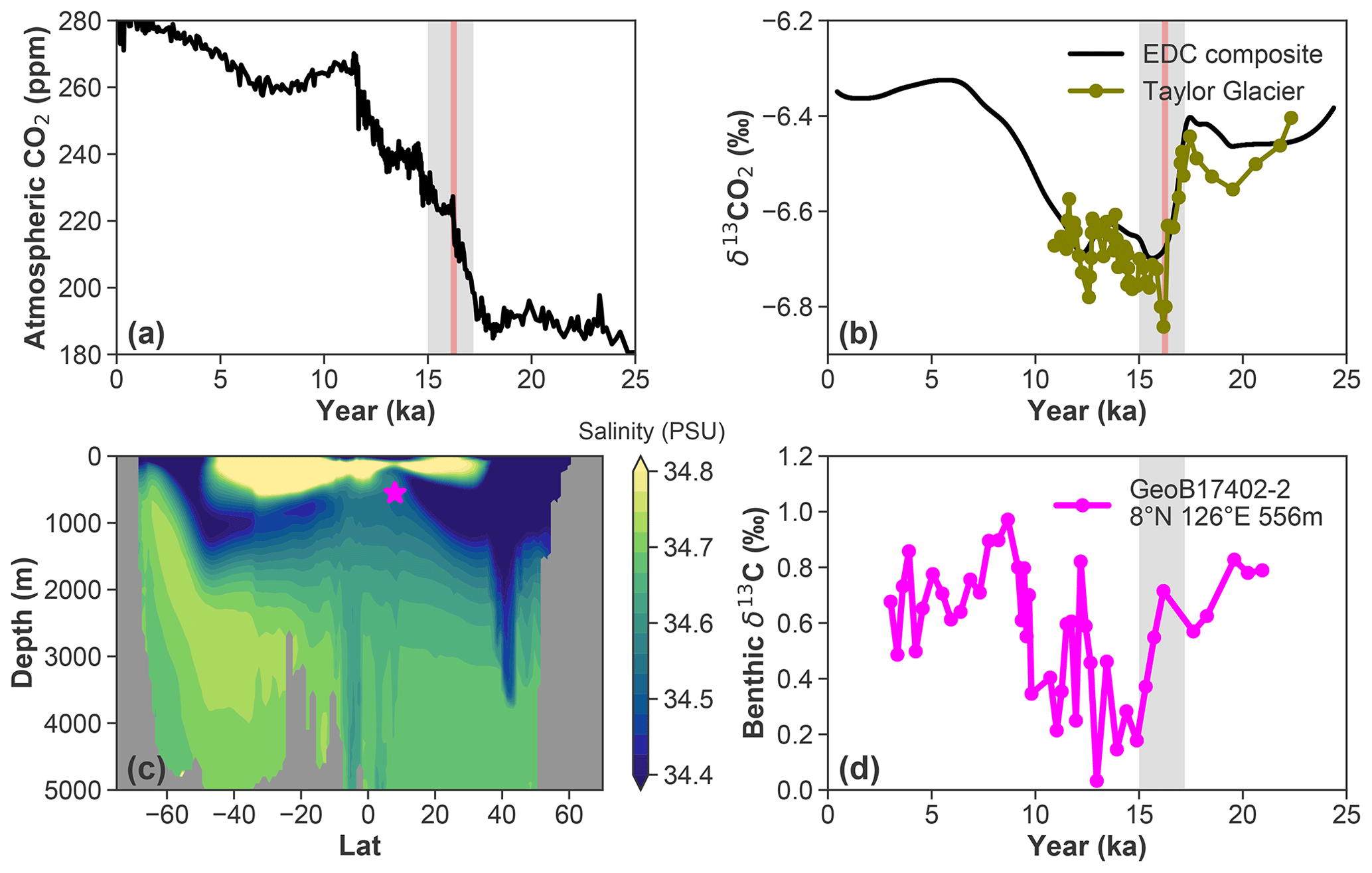
Figure 1(a) Ice core records of atmospheric CO2 (Bereiter et al., 2015; Marcott et al., 2014). (b) δ13CO2 records (Bauska et al., 2016; Schmitt et al., 2012). (c) WOA-18 Pacific zonal mean (120–160∘ E) salinity; the magenta star marks the GeoB17402-2 site. (d) C. mundulus δ13C record for upper-intermediate-depth and mode waters in the western equatorial Pacific. The millennial- and centennial-scale events in these records are highlighted in grey and red, respectively.
Marine proxy records can provide further constraints on the possible mechanisms. For instance, during the early deglaciation, surface and thermocline-dwelling foraminifera around the global ocean also recorded a distinct δ13C drop (e.g., Hertzberg et al., 2016; Lund et al., 2019; Spero and Lea, 2002), an observation replicated by shallow benthic records from the tropical–subtropical Atlantic and Indian oceans (Lynch-Stieglitz et al., 2019; Romahn et al., 2014). These observations have been interpreted to reflect a spread of high-nutrient, low-δ13C waters originating in the Southern Ocean that were subsequently transported throughout the upper ocean via a so-called intermediate water teleconnection (Martínez-Botí et al., 2015; Pena et al., 2013; Spero and Lea, 2002). According to this hypothesis, formerly isolated carbon from deep waters was upwelled in the Southern Ocean (Anderson et al., 2009) in response to a breakdown of deep-ocean stratification (Basak et al., 2018). This carbon would have then been carried by Antarctic Intermediate Water (AAIW) and Southern Ocean Mode Water (SAMW) to low latitudes where it outgassed to the atmosphere in upwelling regions like the eastern equatorial Pacific (EEP). We term this scenario “bottom-up” transport because 13C-depleted carbon passes through the upper ocean globally and is recorded in marine proxy records there before entering the atmosphere (and being recorded in ice cores). The alternative scenario to explain the early deglacial decline in planktic (and shallow benthic) δ13C we term “top-down”. This recognizes the importance of air–sea exchange in rapidly (on the order of 1 year) and globally (e.g., Schmittner et al., 2013) conveying an isotopic signal from the atmosphere to the ocean surface, followed by propagation of the δ13C signal from surface to upper intermediate depths occurring on a multi-decadal to centennial timescale (Heimann and Maier-Reimer, 1996; Broecker et al., 1985; Eide et al., 2017). Although these timescales allow an atmospheric δ13C decline to be propagated throughout the upper ocean, this top-down effect has largely been overlooked in the interpretation of marine planktic and benthic δ13C records, at least until recently (Lynch-Stieglitz et al., 2019).
The implications of the top-down scenario differ significantly from those of the bottom-up scenario. First, negative δ13C excursions recorded in the upper ocean need not be associated with enhanced influx of nutrients (based on the notion that the extra nutrients came from a previously isolated deep-ocean reservoir along with isotopically depleted respired metabolic carbon). Second, a top-down scenario does not require a specific or even a single initial path of carbon into the atmosphere. Outgassing to the atmosphere could occur anywhere at the ocean surface, with a negative δ13C signal that then propagates globally through air–sea gas exchange – akin to the ongoing fossil fuel CO2 emissions and the propagation of their isotopically depleted signal down through the ocean (Eide et al., 2017).
In this paper we take a two-pronged approach to help elucidate the more likely of these end-member scenarios. First, we present a new benthic δ13C record from the western equatorial Pacific (WEP) at a depth of 566 m that fills an important data gap from intermediate water depths in the Pacific basin. The site is located in the pathway of SAMW and AAIW to the upper tropical Pacific (Fig. 1c) and is also shallow enough to be sensitive to δ13CO2 changes in the top-down scenario. Second, the early deglacial section of this record is interpreted with insights gained from analyzing a transient deglacial simulation conducted with the Earth system model LOVECLIM (Menviel et al., 2018). The specific LOVECLIM simulation we utilize starts with a scenario of excess respired carbon accumulated in a more stratified deep ocean with reduced ventilation rates. Although it is not clear if such a glacial carbon scenario is correct (Cliff et al., 2021; Stott et al., 2021), we can still make use of the ability of the model to simulate how the ocean communicates stored carbon and its isotopic composition to the atmosphere during deglaciation (the focus of this paper).
In the transient LOVECLIM simulation, sequestered respired carbon from the deep and intermediate waters is ventilated through the Southern Ocean, leading to a sharp decline in δ13CO2, consistent with ice core records. We evaluate the two different δ13C transport scenarios by partitioning the simulated carbon pool and its stable isotope signature into a preformed (DICpref, being the carbon that is transported passively by ocean circulation) and a respired (DICsoft, the accumulated respired carbon since the water parcel was last in contact with the atmosphere) component. Because the LOVECLIM transient experiment does not explicitly simulate either preformed or respired carbon as additional numerical tracers, the respired carbon is instead estimated by apparent oxygen utilization (AOU) – the difference between oxygen saturation and simulated [O2] (see Sect. 2.4). If the top-down transport scenario was the mechanism responsible for the δ13C decline in marine proxy records from the upper 1000 m of depth, the preformed signal should dominate, while a regenerated signal would dominate in the bottom-up scenario. The carbon partitioning framework is not new – previous studies have used this framework to study the mechanisms that lead to lower glacial atmospheric CO2 (Ito and Follows, 2005; Ödalen et al., 2018; Khatiwala et al., 2019) and processes that control δ13CO2 and marine carbon isotope composition (Menviel et al., 2015; Schmittner et al., 2013). This diagnostic framework has also been applied to study the carbon cycle perturbation in response to a weaker Atlantic Meridional Overturning Circulation (AMOC) (Schmittner and Lund, 2015), albeit in experiments that were performed under constant pre-industrial conditions. However, what is new here is the application of a second Earth system model (cGENIE; Cao et al., 2009) to fully evaluate the AOU-based offline approach against an explicit respired organic matter δ13C tracer.
After describing the new foraminiferal δ13C record in Sect. 2.1, we summarize the LOVECLIM model and a published deglacial transient simulation in Sect. 2.2. We then summarize the cGENIE Earth system modeling framework and deglacial experiments in Sect. 2.3 before describing the δ13C tracer partitioning framework in Sect. 2.4.
2.1 Stable isotope analyses and age model for piston core GeoB17402-2
The WEP piston core GeoB17402-2 (8∘ N, E; 556 m of water depth) (Fig. 1c) was recovered from the expedition SO-228. Planktic foraminiferal samples for 14C age dating were picked from the greater than 250 µm size fraction of sediment samples and were typically between 2 and 5 mg. All new radiocarbon ages were measured at the University of California Irvine Accelerator laboratory. An age model (Fig. S1) was developed for this core with BChron using the Marine20 calibration curve (Heaton et al., 2020) without any further reservoir age correction.
For benthic foraminiferal δ18O and δ13C measurements approximately four to eight Cibicidoides mundulus (C. mundulus) were picked. These samples were cleaned by first cracking the tests open and then sonicating them in deionized water, after which they were dried at low temperature. The isotope measurements were conducted at the University of Southern California on a GV Instruments Isoprime mass spectrometer equipped with an autocarb device. An in-house calcite standard (Ultissima marble) was run in conjunction with foraminiferal samples to monitor analytical precision. The 1 standard deviation for standards measured during the study was less than 0.1 ‰ for both δ18O and δ13C. The stable isotope data are reported in per mil with respect to Vienna Pee Dee Belemnite (VPDB).
2.2 LOVECLIM deglacial transient simulation
The LOVECLIM model (Goosse et al., 2010) consists of a free-surface primitive equation ocean model (, 20 vertical levels), a dynamic–thermodynamic sea ice model, an atmospheric model based on quasi-geostrophic equations of motion (T21, three vertical levels), a land surface scheme, a dynamic global vegetation model (Brovkin et al., 1997), and a marine carbon cycle model (Menviel et al., 2015). To study the sensitivity of the carbon cycle to different changes in oceanic circulation, a series of transient simulations of the early part of the last deglaciation (19–15 ka) (Menviel et al., 2018) was performed by forcing LOVECLIM with changes in orbital parameters (Berger, 1978), changes in the freshwater surface balance and northern hemispheric ice-sheet geometry and albedo (Abe-Ouchi et al., 2007), and starting from an LGM simulation that best fit oceanic carbon isotopic (13C and 14C) records (Menviel et al., 2017).
The simulation we analyzed for this study is “LH1-SO-SHW” from Menviel et al. (2018). We briefly describe the applied forcing in this simulation: first, a freshwater flux of 0.07 Sv was added to the North Atlantic between 17.6 and 16.2 ka, resulting in an AMOC shutdown. Second, a salt flux was added to the Southern Ocean between 17.2 and 16.0 ka to enhance Antarctic Bottom Water (AABW) formation. Due to its relatively coarse resolution, the model could misrepresent the high-southern-latitude atmospheric or oceanic response to a weaker North Atlantic Deep Water (NADW). Enhanced AABW could have occurred due to a strengthening of the SH westerlies, changes in buoyancy forcing at the surface of the Southern Ocean, an opening of polynyas, or sub-grid processes. Finally, two stages of enhanced Southern Ocean westerlies are prescribed in the simulation at 17.2 and at 16.2 ka; this timing generally corresponds to Southern Ocean warming associated with two phases of NADW weakening during Heinrich Stadial 1 (Hodell et al., 2017). For further details about this experiment, see Menviel et al. (2018).
We chose to focus our analysis on this particular simulation because (1) recent ice core records also suggest enhanced SO westerly winds during Heinrich stadials (Buitzert et al., 2018); (2) LH1-SO-SHW matches some of the important observations (e.g., ice core record of atmospheric CO2 and δ13CO2) better than the other scenarios presented in Menviel et al. (2018); and (3) the stronger SO wind stress in LH1-SO-SHW leads to an increased transport of AAIW to lower latitudes, which could have impacted the intermediate depths of the global ocean.
2.3 cGENIE simulations
The cGENIE Earth system model is based on a 3-D frictional geostrophic ocean circulation component, plus dynamic and thermodynamic sea ice components, and is configured here at a 36×36 horizontal grid resolution with 16 vertical layers in the ocean. The configuration we employ here lacks a dynamical (GCM) atmosphere, with atmospheric transport fixed and provided via a 2-D energy–moisture balance model (Edwards and Marsh, 2005). The low-resolution ocean component and highly simplified atmospheric component make cGENIE much less computationally expensive to run than LOVECLIM and facilitate multiple sensitivity experiments run to (deep-ocean circulation) steady state to help partition and attribute carbon sources and pathways.
Ocean carbon storage analysis using the cGENIE model has previously utilized a range of preformed tracers, including those of phosphate (Ppref), dissolved inorganic carbon (DICpref), dissolved oxygen (O2pref), and alkalinity (Ödalen et al., 2018). In the model, these are implemented by resetting the current value of the tracer at the ocean surface at each time step to the corresponding “full” tracer; for example, the value of DICpref is set to that of surface ocean DIC. Technically, an anomaly is applied to each preformed tracer at the ocean surface at each time step, equal to the difference between the current bulk tracer value and the preformed tracer value (as opposed to simply directly setting the values equal in the code). Because in the numerical scheme, all fluxes, including those induced by ocean circulation and any preformed tracer anomalies, are calculated simultaneously and only summed and applied to update the tracer concentration field at the very end of the model time step, preformed tracer concentrations at the ocean surface and at the end of the time step never exactly equal those of the bulk tracer. Thereafter, these tracers are carried conservatively by ocean circulation, with no loss or gain due to, for instance, organic matter remineralization in the ocean interior.
We expand the diagnostic tracer capabilities of cGENIE here and additionally add DICsoft, which is the contribution to DIC from respired carbon. This is implemented as a tracer reset to zero at the ocean surface at each time step, but which is incremented by an amount of DIC equal to the remineralization of both particulate and dissolved organic matter and including organic carbon “reflected” (not preserved and buried) from the sediment surface. As for the preformed tracers, ocean circulation also acts on the distribution of DICsoft in the model. Figure S2 in the Supplement illustrates how DIC is partitioned for the pre-industrial steady state of Cao et al. (2009). Note that we do not explicitly simulate DICcarb (the contribution to DIC from dissolving CaCO3, either in the water column or at the sediment surface) as a fourth tracer, but rather simply calculate it as the difference between DIC and DICpref+DICsoft.
We also create a novel addition to the model – preformed and respired 13C (δ13Cpref and δ13Csoft, respectively). These are implemented as DICpref and DICsoft, except for the concentrations of DI13C. (In cGENIE, isotopes are carried explicitly as concentrations with delta (δ) values only generated in conjunction with bulk concentrations for output and more convenient input.) Figure S3 illustrates how the δ13C signature of DIC is partitioned into explicitly simulated preformed and respired carbon components, with δ13Ccarb (the contribution to δ13C of DIC from dissolved CaCO3) again calculated by difference.
A full description of the cGENIE tracer scheme, together with δ13C tracer decomposition and attribution error analysis for both steady-state carbon cycling and under an idealized perturbation experiment, is available in the Supplement, with the pertinent insights summarized in the Results section.
Finally, we create a transient deglacial-like experiment using cGENIE to approximately mimic some of the key features of a changing climate and carbon cycle simulated by LOVECLIM. Although AOU-based errors in estimating the partitioning of respired vs. preformed δ13C are already addressed via the idealized cGENIE steady-state and transient experiments (the Supplement), decoupling in time of atmospheric CO2 (and δ13C), surface climate, biological export, and the large-scale circulation of the ocean (especially the AMOC) across the deglacial transition may induce a more complex evolution of AOU-based error. We address this by then calculating how the AOU-based error changes in a deglacial-like cGENIE experiment. For this, we take a model configuration based on the idealized “glacial” boundary conditions of Rae et al. (2020) (including increased zonal planetary albedo at high Northern Hemisphere latitudes and the orbital configuration at 21 ka). Note that we did not attempt to achieve a glacial-like atmospheric CO2 value for this spin-up; instead, we prescribed atmospheric CO2=278 ppm and ‰. The spin-up was run for 10 000 years. We then performed a deglacial transient simulation with time-varying salt–freshwater flux into the North Atlantic and the Southern Ocean as well as wind stress forcing over the Southern Ocean (Fig. S8 in the Supplement). We ran this experiment with all the diagnostic tracers described above.
2.4 Separating δ13C anomalies into the preformed (Δδ13Cpref) and respired (Δδ13Csoft) component
The published (Menviel et al., 2018) transient LOVECLIM model experiment that we analyze here does not include the numerical tracers required to explicitly attribute the sources of any given change in δ13C in the model ocean. We hence make approximations from AOU calculated in the model experiment but assess the errors inherent in this by means of a set of experiments using a second Earth system model – cGENIE (Cao et al., 2009). This approach is detailed as follows (and expanded upon further in the Supplement).
We assume the following carbon isotopic mass balance:
where DIC, DICpref, DICsoft, and DICcarb are the dissolved total inorganic carbon, the preformed and respired organic matter (“Csoft”), and dissolved (calcium) carbonate carbon pools, respectively. δ13Cpref, δ13Csoft, and δ13Ccarb are the corresponding isotopic signatures (as ‰) that contribute to the δ13C signature of DIC, and it is changes in the δ13C of DIC that we assume foraminiferal records reflect.
Any given observed δ13C anomaly in the ocean can then be expressed as follows:
The terms on the right-hand side (RHS) represent the contribution of the preformed, respired, and dissolved (carbonate) components to the overall δ13C change, respectively. Since the contribution of CaCO3 dissolution is small in the upper 1000 m (where GeoB17402-2 is located) in carbon cycle models (see also the Supplement) and since there is no 13C fractionation during CaCO3 formation in the LOVECLIM model, the last term on the RHS can be neglected for the purpose of this study.
We use AOU to estimate respired carbon and its contribution to the δ13C changes: , where δ13Csoft is estimated by the δ13C of export particulate organic carbon (POC) in the overlying water column and .
This leads to
The anomaly, defined as the difference between 15 and 17.2 ka, can be expanded as follows.
The AOU approach to estimate respired carbon content assumes that the oxygen content of surface waters always reaches equilibrium with the overlying atmosphere. However, studies have shown that this is not always the case, particularly for water masses formed in high latitudes (Bernardello et al., 2014; Ito et al., 2004; Khatiwala et al., 2019; Cliff et al., 2021). As a result, AOU likely overestimates respired carbon content in the deep ocean. Additional errors associated with the AOU approach may result from the nonlinear solubility of O2 and respiration that does not involve O2 consumption (i.e., through denitrification or sulfate reduction) (Shiller, 1981; Ito et al., 2004). However, to what extent these biases will affect the relative contribution of the preformed and respired carbon pool to δ13C anomalies in a carbon cycle perturbation event has not to our knowledge previously been evaluated. To address this, we performed a deglacial transient simulation with cGENIE (see Sect. 2.3) and then applied Eq. (4) to the output, with the results then compared with the values that are explicitly simulated by cGENIE. We also conducted a simplified (modern-configuration-based) analysis of steady-state and transient error terms (Figs. S2–S7), which we include in full in the Supplement and discuss briefly in the main text.
The new GeoB17402-2 benthic δ13C record from the intermediate WEP documents a −0.3 ‰ to −0.4 ‰ decline during the early deglaciation (Fig. 1d). Although the foraminiferal δ13C proxy can be complicated by temperature and carbonate ion changes (Bemis et al., 2000; Schmittner et al., 2017) and may thus not solely reflect seawater DIC δ13C changes, core-top patterns of benthic foraminiferal δ13C are highly correlated with present-day seawater DIC δ13C (Schmittner et al., 2017). The apparent lag between the onset of decline in benthic δ13C at site GeoB17402-2 (Fig. 1d) and in δ13CO2 appears to be due to the relatively large age model uncertainty below 154 cm in the GeoB17402-2 record (median age ∼16.2 years) of up to 1–2 kyr (2 SD) (Fig. S1). Despite this age uncertainty, the new benthic record from the tropical Pacific captures a similar δ13C decline as recorded from similar depth sites in the tropical–subtropical Atlantic and Indian oceans (Lynch-Stieglitz et al., 2014, 2019; Romahn et al., 2014).
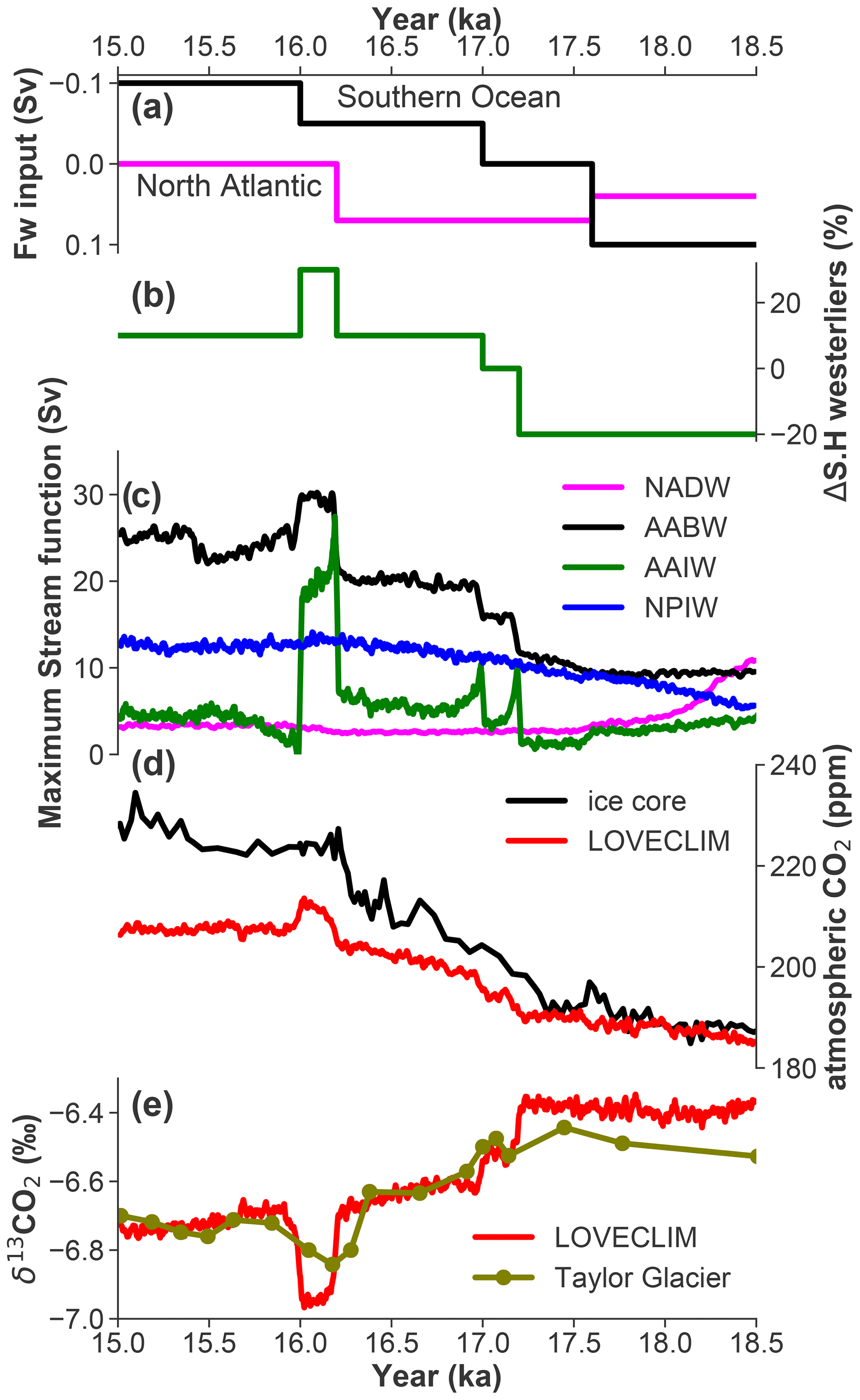
Figure 2Time series from the LOVECLIM transient experiment (Menviel et al., 2018). (a) Freshwater input into the North Atlantic and the Southern Ocean. (b) Southern Hemisphere westerly wind forcing. (c) Simulated NADW, AABW, AAIW, and NPIW maximum stream function in LOVECLIM; 21-year moving averages are shown for the maximum stream function to filter the high-frequency variability. (d) Ice core record of atmospheric CO2 (Bereiter et al., 2015; Marcott et al., 2014) and LOVECLIM-simulated atmospheric CO2. (e) The Taylor glacier δ13CO2 record (Bauska et al., 2016) and LOVECLIM-simulated δ13CO2.
To investigate whether the early deglacial δ13C decline observed at these sites in the upper ocean is dominated by the preformed or respired component, we carried out an in-depth carbon cycle analysis of the LOVECLIM transient simulation (Menviel et al., 2018). In response to the applied freshwater input to the North Atlantic (Fig. 2a), the AMOC significantly weakens from its glacial state (Fig. 2c). This has only a minor effect on the atmospheric CO2 and δ13CO2 (Fig. 2d and e). In contrast, enhanced ventilation of AABW and AAIW caused by a combined freshwater- (Fig. 2a) and wind-stress-driven (Fig. 2b) breakdown of stratification leads to an atmospheric CO2 increase of ∼25 ppm and δ13CO2 decline of −0.35 ‰ between 17.2 and 15 ka (Fig. 2d and e). This is a consequence of stronger upwelling, bringing 13C-depleted deep waters to the upper ocean with δ13C generally decreasing by 0.2‰–0.3‰ at most locations in the upper 1000 m (Fig. 3a, d, and g). In all sectors of the Southern Ocean below a depth of 400 m, δ13C increases by 0.1‰–0.2‰ due to stronger ventilation. Throughout the mid-depth North Atlantic, δ13C decreases by more than 0.3‰–0.4‰ due to the weakening AMOC (Fig. 3g). Finally, the LOVECLIM simulates a North Pacific deepwater mass when AMOC slows down (Menviel et al., 2014), and this leads to stronger ventilation and +0.3‰–0.4‰ Δδ13C in the North Pacific below depths of 1000 m (Fig. 3a).
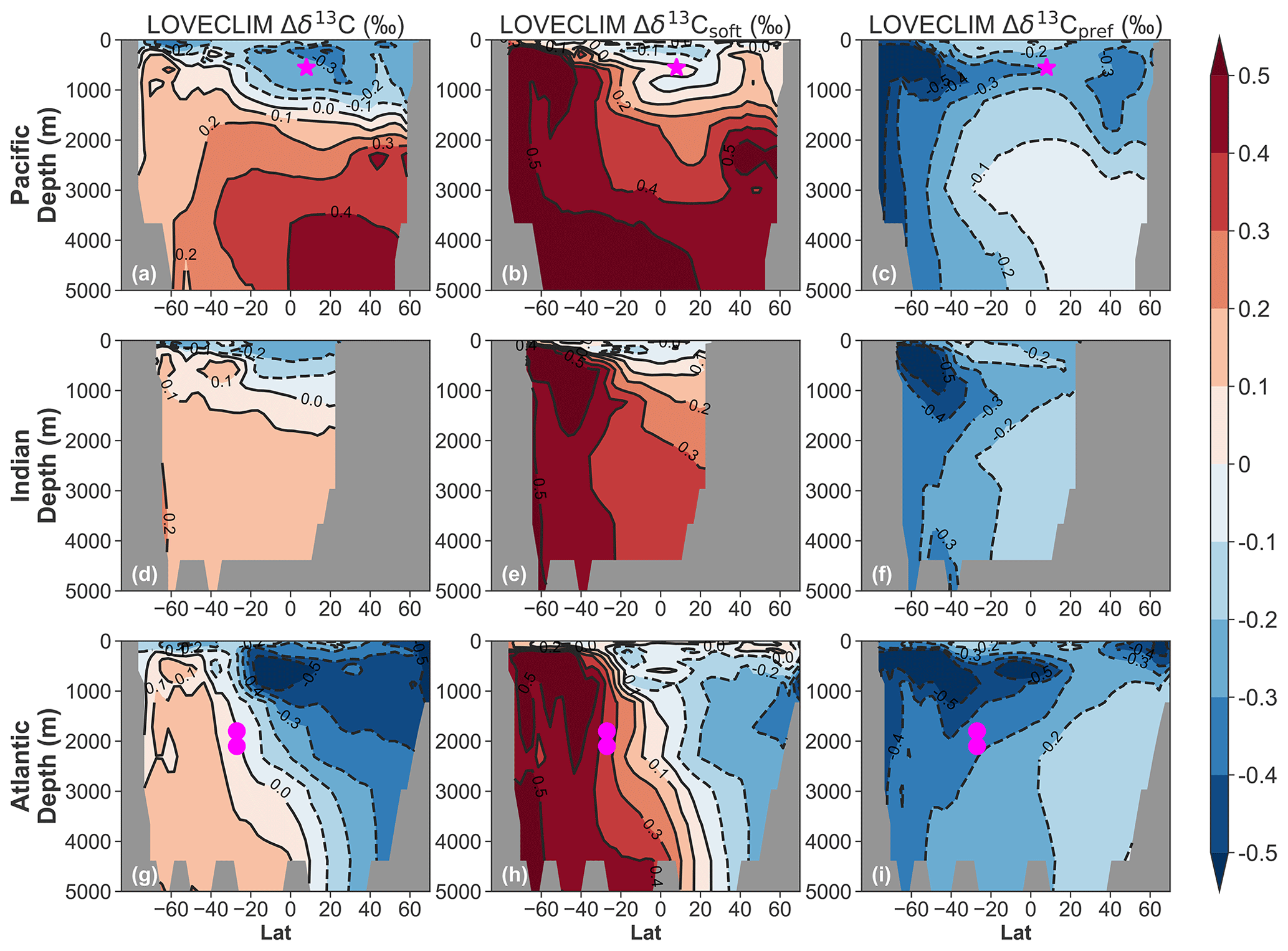
Figure 3Ocean basin zonal mean anomalies (15 ka minus 17.2 ka) as simulated in LOVECLIM. (a–c) Pacific zonal mean anomaly (160∘ E–140∘ W). The magenta star marks the GeoB17402-2 site. (d–f) Indian zonal mean anomaly (50–90∘ E). (g–i) Atlantic zonal mean anomaly (60–10∘ W). The magenta circles mark the 78GGC and 33GGC sites discussed in Sect. 4.3.
Decomposing the LOVECLIM Δδ13C signal into the Δδ13Csoft and Δδ13Cpref component, we find that the entire water column of the Southern Ocean is characterized by a strong positive Δδ13Csoft (indicting a loss of respired carbon) and a strong negative Δδ13Cpref (Fig. 3b, c, e, f, h, and g). In the rest of the global upper ocean below depths of 1000 m, Δδ13Csoft is negative but of a magnitude smaller than 0.1 ‰, whereas a 0.2‰–0.3‰ decrease in Δδ13Cpref accounts for most of the Δδ13C signal. In the deep Indo-Pacific, Δδ13Csoft and Δδ13Cpref show opposite signs, with the positive Δδ13Csoft dominating the net Δδ13C (Fig. 3a–f). In the deep North Atlantic, Δδ13Csoft and Δδ13Cpref are both negative (Fig. 3h and i), leading to the largest decrease in Δδ13C across the ocean basins (Fig. 3g).
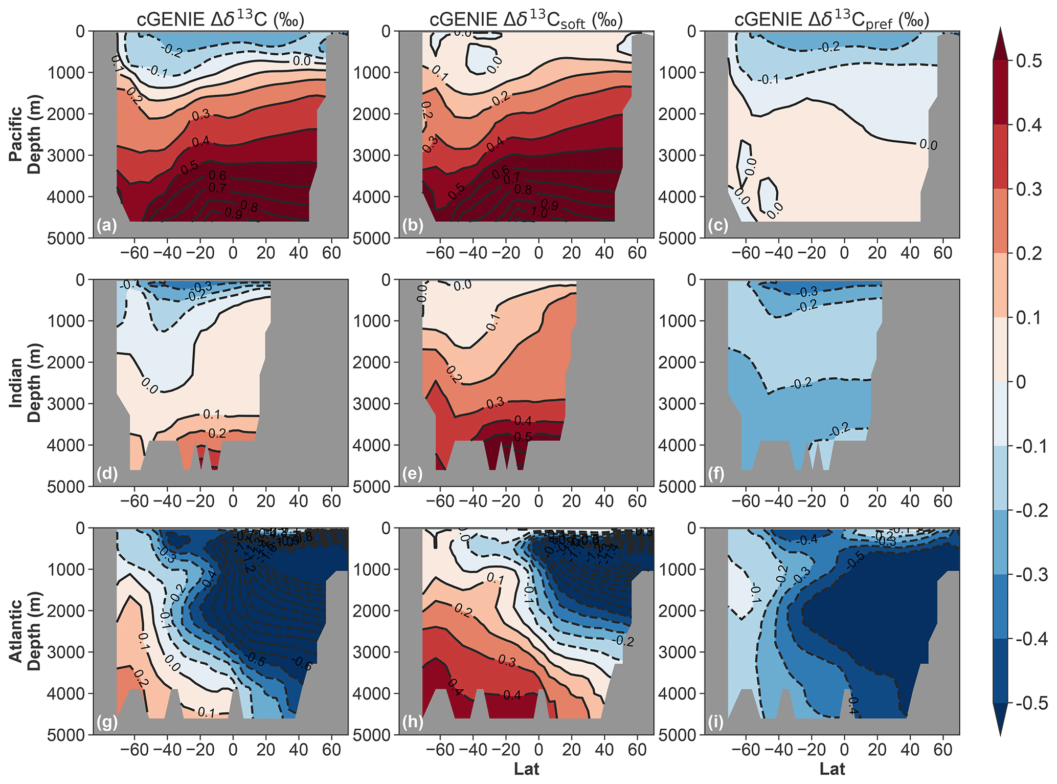
Figure 4Ocean basin zonal mean anomalies (15 ka minus 17.2 ka), but for the cGENIE deglacial transient simulation. Panels are organized as in Fig. 3.
For comparison, Fig. 4 shows the Δδ13C, Δδ13Csoft, and Δδ13Cpref response in a similar deglacial-like transient simulation conducted with cGENIE (see Sect. 2.3 and Fig. S8) in which the respired and preformed components are explicitly simulated. The Δδ13C patterns (Fig. 4a, d, and g) are qualitatively similar to that simulated by LOVECLIM (Fig. 3a, d, and g), although the magnitude of positive Δδ13C in the deep Pacific and negative Δδ13C in the deep North Atlantic is larger in cGENIE (compare Fig. 3a with Fig. 4a and Fig. 3g with Fig. 4g). cGENIE does not simulate any large positive Δδ13Csoft or negative Δδ13Cpref in the Southern Ocean above depths of 3000 m (Fig. 4), in contrast to the AOU-based results from LOVECLIM (Fig. 3). In the North Atlantic, the magnitudes of negative Δδ13Csoft and Δδ13Cpref are both larger in cGENIE compared to LOVECLIM.
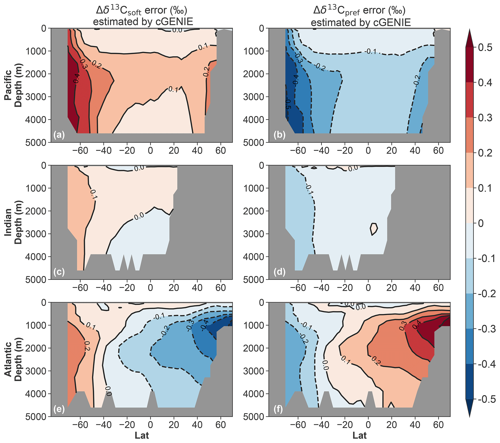
Figure 5cGENIE early deglacial transient AOU error analysis for Δδ13Csoft (a, c, e) and Δδ13Cpref (b, d, f). The anomalies are defined as 15 ka minus 17.2 ka. The errors are defined as AOU-based anomaly minus explicitly simulated anomaly.
To assess the potential errors associated with the AOU-based approach used to process the LOVECLIM output, we also calculated AOU-derived estimates of Δδ13Csoft and Δδ13Cpref for the cGENIE deglacial transient simulation (see Sect. 2.4). The results suggest that throughout the mid-depth North Atlantic, the AOU-based Δδ13C decomposition may introduce errors up to 0.3‰–0.4‰ under a weakening of the AMOC (Fig. 5). In the Southern Ocean (south of 40∘ S), the AOU-based approach overestimates the magnitude of the positive Δδ13Csoft and negative Δδ13Cpref by 0.1‰–0.4‰ (Fig. 5); the largest errors occur in the Pacific sector. Based on these results from cGENIE, we suggest that the apparent Δδ13Csoft and Δδ13Cpref in the Southern Ocean shown in the LOVECLIM decomposition (Fig. 3) are largely overestimated. Nonetheless, both cGENIE and LOVECLIM (after correcting the errors estimated from the cGENIE deglacial transient experiment; see Fig. 5) show that the preformed component contributes −0.1‰ to −0.2 ‰ to the total Δδ13C signal in the upper 1000 m of the Southern Ocean. To the north of 40∘ S in the upper 1000 m of the global upper ocean (except for the upper North Atlantic), the errors are relatively minor (generally much less than 0.1 ‰ in magnitude) and the AOU-based approach can provide a reasonably good estimate (Fig. 5, also Figs. S5 and S7).
Finally, we further evaluate the errors inherent in the AOU-based approach for the decomposition of the different contributions to the δ13C changes by means of a series of idealized steady-state and transient cGENIE experiments, as described in the Supplement. From this we find that errors in estimating δ13Csoft arise from both errors in AOU (themselves composed of errors due to assuming air–sea equilibrium and because O2 solubility increases nonlinearly with decreasing temperature) and the assumption that the isotopic signature of carbon released by the remineralization of organic matter at any location in the ocean reflects that of carbon exported from the directly overlying ocean surface. The latter error turns out to be small in LOVECLIM as a consequence of its relatively small (3 ‰) simulated latitudinal variability in organic matter δ13C, leaving the better understood AOU-driven error to dominate the net uncertainty in reconstructing δ13Csoft. As a further consequence of this, under idealized transient changes in climate and ocean circulation in cGENIE (see the Supplement), the AOU-induced error in δ13Csoft is almost invariant throughout the uppermost ca. 500 m of the ocean, simply because the error in AOU itself is close to zero here. This confirms the conclusions drawn from tracer comparisons made in deglacial cGENIE experiments that at the depth of GeoB17402-2, the AOU-based approach is relatively robust.
4.1 Atmospheric δ13C bridge
In the LOVECLIM model 13C-depleted carbon is ultimately sourced from the respired carbon that accumulated in the deep and intermediate waters during the glacial period as a consequence of the imposed weakened deepwater formation (Menviel et al., 2017). We show that in this scenario the isotopic signal is first transmitted to the atmosphere through strong outgassing in the Southern Ocean (Fig. 6). The atmosphere then transmits the δ13C signal to the rest of the global surface and subsurface ocean through air–sea gas exchange. An illustrative example is the simulated transient δ13C minimum event between 16.2 and 15.8 ka in LOVECLIM (Fig. 2c), which originates from the Southern Hemisphere and specifically from enhanced ventilation of AAIW (Fig. 2a). In the model, if the top-down scenario is true, the upper water masses away from the Southern Hemisphere would show a similar magnitude of δ13CDIC changes as δ13CO2. On the other hand, if the bottom-up scenario is true, a large negative δ13C anomaly (of respired nature) should first appear in the South Pacific subtropical gyre (STGSP), as the STGSP lies on the pathway between Southern Ocean water masses and those at lower latitudes. Then the signal would progressively spread to the tropics and finally reach the North Pacific. The negative δ13C anomaly may also be gradually diluted along its pathway from the South Pacific to the North Pacific. However, in the LOVECLIM simulation, there is no δ13C minimum in the upstream STGSP, while the atmosphere-like negative δ13C anomaly appears in the EEP thermocline, the North Pacific subtropical gyre (STGNP), and North Pacific Intermediate Water (NPIW) simultaneously (Fig. 7). In addition, the millennial-scale δ13C evolution in these upper-ocean water masses to the north of the Equator exhibits a pattern of change that is similar to that of the atmosphere (Fig. 7). The synchronized δ13C changes therefore point to the dominant role of atmospheric communication rather than time-progressive oceanic transport of a low δ13C signal in LOVECLIM.
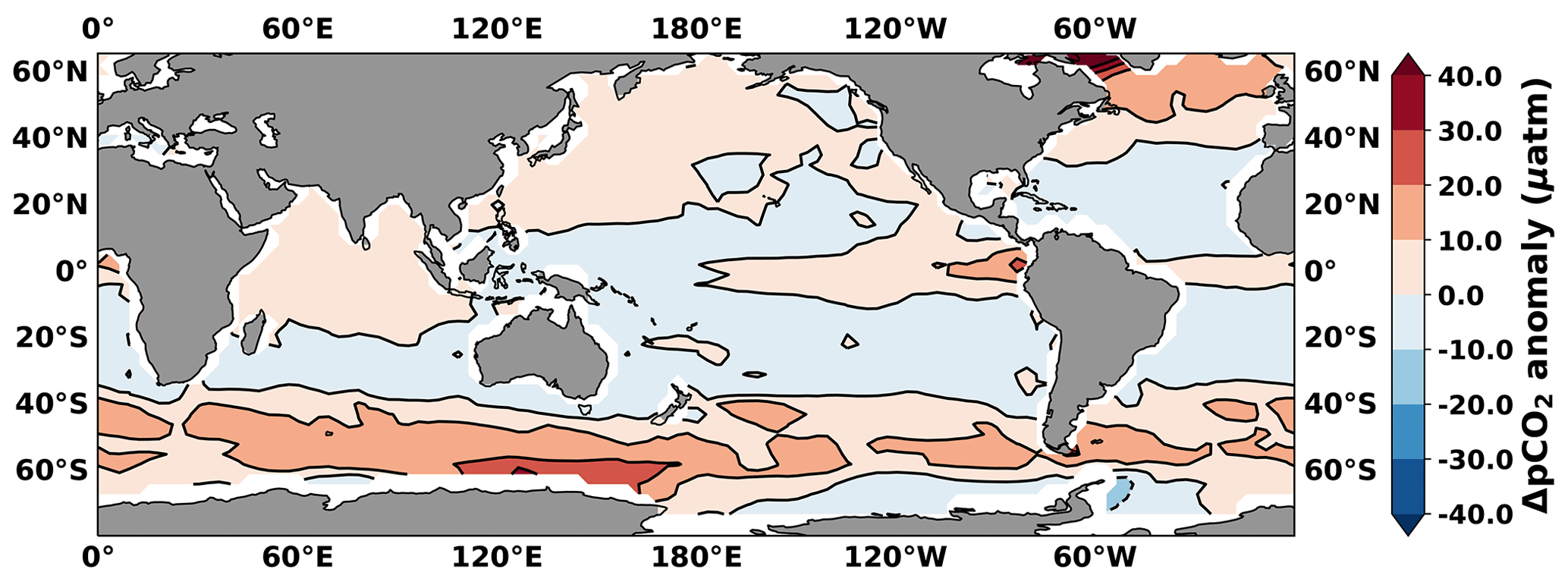

Figure 7LOVECLIM-simulated Δδ13C in thermocline the EEP (90–82∘ W, 5∘ S–5∘ N; 77–105 m), South Pacific subtropical gyre (STGSP; 160∘ E–100∘ W, 40–22∘ S; 187–400 m), North Pacific subtropical gyre (STGNP; 110∘ E–140∘ W, 22–40∘ N; 187–400 m), and NPIW (167–170∘ E, 54–57∘ N; 660 m). The average of 23.8–20 ka (i.e., LGM) is used as a reference level for the Δδ13C calculations. The interval of decreasing δ13C is highlighted with a grey bar.
In the LOVECLIM simulation, both millennial- and centennial-scale δ13CO2 declines are the result of enhanced deep-ocean and/or intermediate ocean ventilation originating in the Southern Ocean. Using the UVic Earth system model, Schmittner and Lund (2015) showed that a slowdown of AMOC alone is able to weaken the global biological pump and lead to light carbon accumulation in the upper ocean and the atmosphere, without explicitly prescribing any forcing in the Southern Ocean. Despite the different prescribed forcing, Δδ13Cpref also dominates the total Δδ13C in the upper 1000 m of the global ocean in the UVic experiment (see Fig. 6 in Schmittner and Lund, 2015). Taken together, simulations by all three models suggest that any process that lowers atmospheric δ13CO2 would influence the global upper-ocean δ13C. In fact, the same phenomenon has been recurring since the beginning of the industrial era due to fossil fuel burning – known as the Suess effect (Eide et al., 2017). The top-down scenario is also compatible with the concept of a nutrient teleconnection between the Southern Ocean and low latitudes (Palter et al., 2010; Pasquier and Holzer, 2016; Sarmiento et al., 2004). Figure 8 illustrates that stronger upwelling brings excess nutrients to the surface of the Southern Ocean. Unused nutrients are then transported to low latitudes within the upper-ocean circulation (e.g., through mode waters and thermocline waters). However, a nutrient teleconnection does not, in itself, reflect an enhanced flux of 13C-depleted DIC from the deep ocean to low latitudes in a “tunnel-like” fashion (and bottom-up transport).
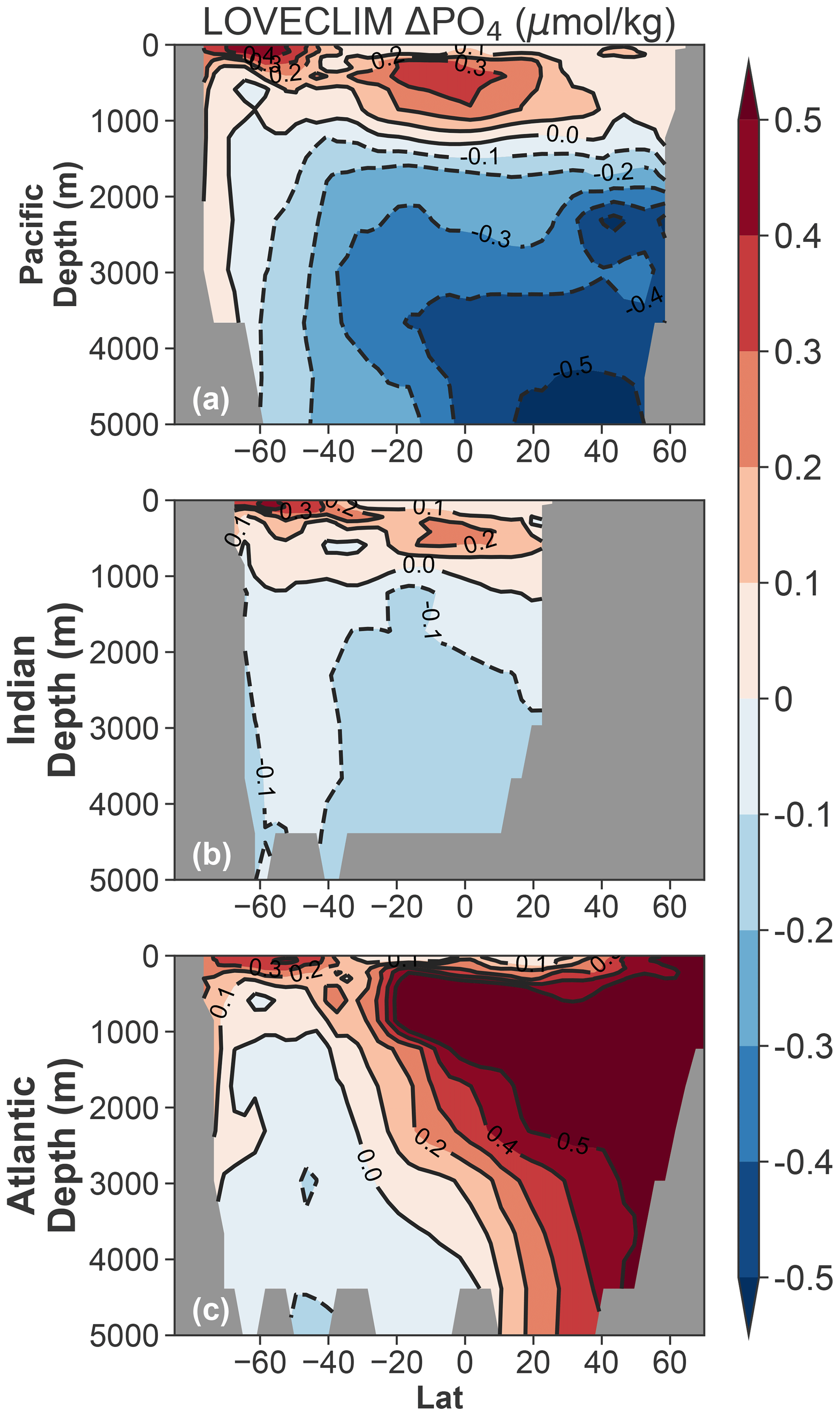
Figure 8Ocean basin zonal mean PO4 anomalies (15 ka minus 17.2 ka) as simulated in LOVECLIM.
In the following sections, we present two cases in which the LOVECLIM transient simulation successfully captures the early deglacial δ13CDIC evolution recorded in marine proxies. The model-based Δδ13C partitioning then offers a unique opportunity to investigate the controlling mechanisms of the observed marine δ13C variability. We acknowledge that there are also places where models (in both LOVECLIM and cGENIE deglacial transient simulations) fail to simulate the observed δ13C trend between 17.2 and 15 ka. For instance, models simulate significant positive Δδ13C (above 0.4‰–0.5‰) (Figs. 3a and 4a) in the deep tropical North Pacific, whereas observations record no significant trend (Lund and Mix 1998; Stott et al., 2021). Models also simulate very small Δδ13C (∼0.1 ‰) in the deep tropical northern Indian Ocean (Figs. 3d and 4d), whereas proxy records document a distinct +0.3‰–0.4‰ trend (Waelbroeck et al., 2006; Sirocko, 2000). The model–data disagreement in the deep Indo-Pacific warrants future study.
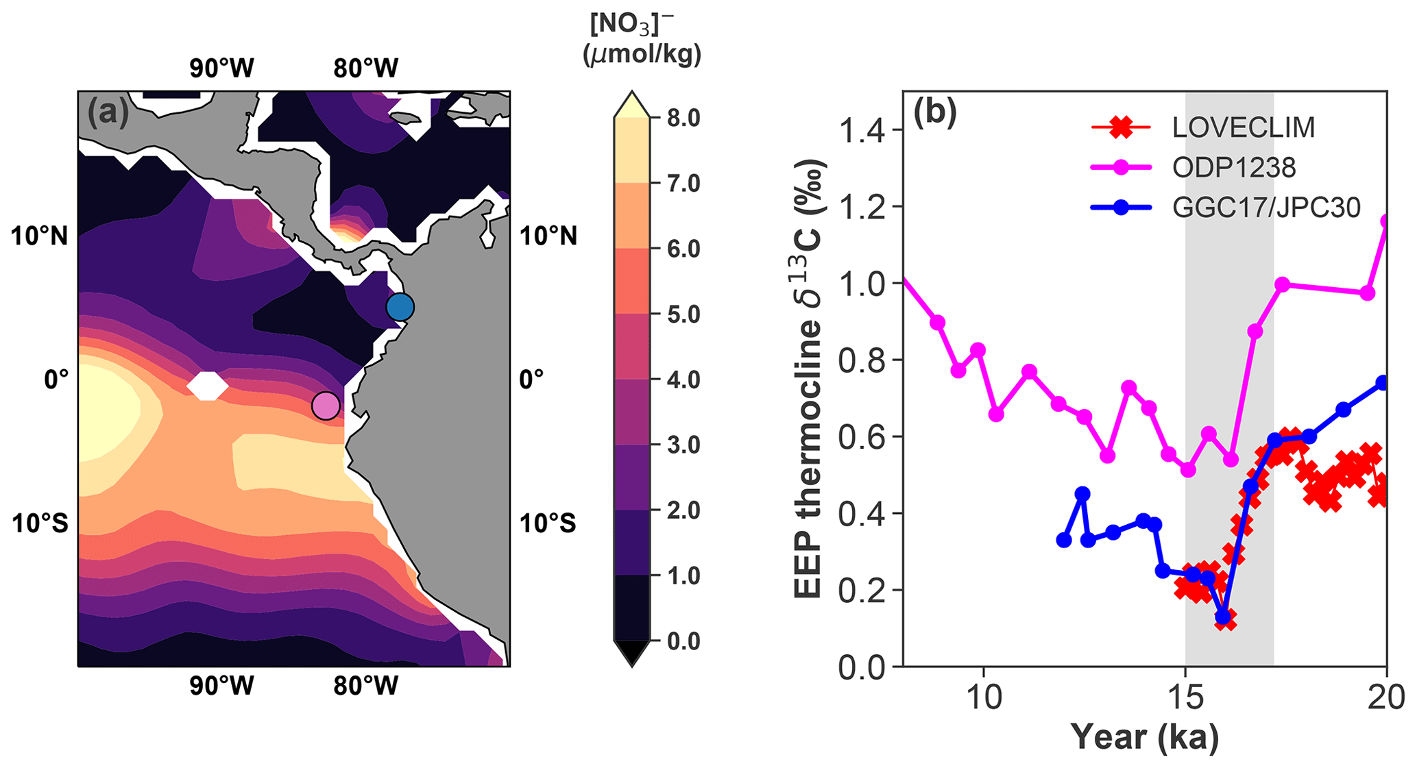
Figure 9(a) Modern sea surface nitrate concentration from the WOA-18 dataset. The sites of ODP 1238 and GGC17/JPC30 are marked as a purple and blue circle, respectively. (b) Neogloboquadrina dutertrei (N. dutertrei, a shallow thermocline species) δ13C data from ODP 1238 (Martínez-Botí et al., 2015) and GGC17/JPC30 (Zhao and Keigwin, 2018), as well as LOVECLIM-simulated δ13C of DIC at 100 m (average of 82–90∘ W, 5∘ S–5∘ N). The N. dutertrei data are corrected by −0.5 ‰ to normalize to δ13C of DIC (Spero et al., 2003). The grey shaded bars highlight the time period we focus on in this study.
4.2 Revisiting EEP thermocline δ13C
Waters at EEP thermocline depths are thought to be connected to the deep ocean through AAIW from the south and NPIW from the north. The EEP is therefore a potential conduit for deep-ocean carbon release to the atmosphere. On the other hand, the EEP thermocline is also shallow enough to record an atmospheric δ13C signal, either directly through gas exchange at the surface or indirectly through a preformed signal acquired from other parts of the global surface ocean. We select two EEP thermocline δ13C records from different oceanographic settings (Fig. 9a): site GGC17/JPC30 is near the coast, featuring relatively low surface nutrients; site ODP1238 is located in the main upwelling zone, with relatively high surface nutrients. Previous studies suggest that the deglacial histories of deepwater influence at the two sites were also distinctively different. At site ODP1238, strengthened deglacial CO2 outgassing inferred from boron isotope data has been interpreted to reflect respired carbon transported from the Southern Ocean (Martínez-Botí et al., 2015); at site GGC17/JPC30, wood-constrained constant surface reservoir ages over the last 20 kyr suggest that this site was not influenced by old respired carbon from high latitudes (Zhao and Keigwin, 2018). However, the early deglacial planktic δ13C records from the two sites show remarkably similar evolution, which is well captured by the LOVECLIM transient simulation (Fig. 9b). By comparing Fig. 3b and c, it is clear that the simulated δ13C anomaly in the EEP thermocline (∼100 m) is dominated by the preformed component. The modeling evidence indicates that even though the EEP is the largest CO2 outgassing region (in terms of absolute ΔpCO2; Fig. S9) under an enhanced Southern Ocean upwelling scenario, its thermocline δ13C is dominantly controlled by the top-down mechanism rather than the bottom-up mechanism as previously suggested (Martínez-Botí et al., 2015; Spero and Lea, 2002). The apparent conundrum can be explained by the fact that the air–sea balance of carbon isotopes is achieved through gross rather than net CO2 exchange. Collectively, we make the case that in strong upwelling regions (e.g., the EEP) that are remotely connected to the deep ocean, thermocline δ13C is still subjected to strong atmospheric overprint.
4.3 How deep in the ocean can the negative Δδ13Cpref signal from the atmosphere penetrate during the early deglaciation?
We have shown that given the dominant control of the preformed δ13C component in the upper ocean, some interpretations of planktic δ13C records might need to be re-evaluated. Our simulations also reveal that an atmospheric influence can extend beyond thermocline depths into upper intermediate depths – consistent with what Lynch-Stieglitz et al. (2019) proposed. Below 1000 m, a Δδ13Cpref signal from the atmosphere may still exist, but it no longer dominates the total Δδ13C as Δδ13Csoft becomes increasingly important at depth. (The contribution of δ13Ccarb also increases at depth and can exceed 10 % of the contribution of δ13Csoft; see Fig. S3.)
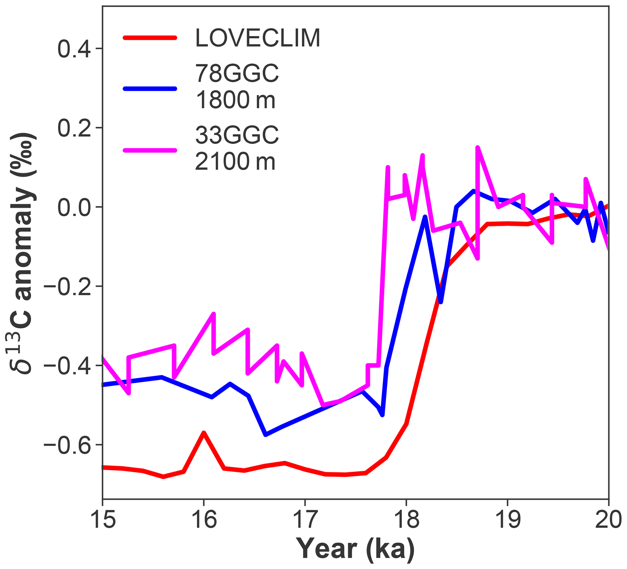
Figure 10Observed δ13C anomaly of 78GGC and 33GGC from the mid-depth of the Brazil Margin at 27∘ S (Lund et al., 2015) and the LOVECLIM-simulated δ13C anomaly at this location.
It has been suggested that deglacial δ13C variability in the waters above a depth of 2000 m in the Atlantic could be driven by air–sea exchange (Lynch-Stieglitz et al., 2019). However, mid-depth (1800–2100 m) benthic δ13C records from the Brazil Margin (∼27∘ S) document a sharp decline of 0.4 ‰ at ∼18 ka (Lund et al., 2019), while atmospheric δ13CO2 did not decrease until ∼17 ka (Bauska et al., 2016; Schmitt et al., 2012). Lund et al. (2019) argued that the lagging atmospheric δ13CO2 decline seemed at odds with the idea that δ13Cpref contributed to the early benthic δ13C decrease at their site. The observed benthic δ13C trend between 20 and 15 ka at these Brazil Margin sites is well simulated by LOVECLIM (Fig. 10), allowing us to explore this question further. Before atmospheric δ13CO2 starts to decline in LOVECLIM at ∼17.2 ka, changes in δ13CDIC at a depth of ∼2000 m at the Brazil Margin are dominantly controlled by excess accumulation of respired carbon (indicated by highly negative Δδ13Csoft; Fig. S10b), itself a response to the weakened AMOC, while Δδ13Cpref is relatively small (Fig. S10c). This is consistent with what previous studies have suggested (Lacerra et al., 2017; Lund et al., 2019; Schmittner and Lund, 2015). Interestingly, LOVECLIM also reveals a strong negative Δδ13Cpref signal between 17.2 and 15 ka when atmospheric δ13CO2 declines (Fig. 3i). However, a positive Δδ13Csoft (Fig. 3h) signal originating from a loss of respired carbon due to enhanced ventilation at those depths almost completely compensates for the negative Δδ13Cpref, which leads to virtually no net change in δ13CDIC in the simulation (Fig. 3g), consistent with the proxy observations (Fig. 10). These results suggest that, between 17.2 and 15 ka, a negative preformed δ13C signal from the atmosphere needs to be considered when interpreting benthic δ13C records from the upper 2000 m of the South Atlantic. The complexity associated with interpreting marine δ13C records further underscores the urgent need to develop more robust means of estimating respired carbon accumulation or release from water masses.
A transient simulation conducted by the LOVECLIM Earth system model is used as a realization of plausible pathways of low-δ13C-signal transport under a prevailing deglacial scenario that involves Southern Ocean processes. By applying an AOU-based partitioning of carbon isotopic changes into preformed and respired components – a methodology that we scrutinize via a series of additional cGENIE Earth system model experiments – we show that ocean–atmosphere gas exchange likely dominates the negative δ13C anomalies documented in global planktic and intermediate benthic δ13C records between 17.2 and 15 ka. Numerical simulations further suggest that enhanced Southern Ocean upwelling can transfer δ13C signals from respired carbon in the deep ocean directly to the atmosphere. Consequently, atmospheric δ13CO2 declines and this leaves its imprint on the rest of the global upper ocean through air–sea exchange. The preformed component dominates the upper 1000 m and could account for a 0.3‰–0.4‰ decline in marine δ13C records during the early deglaciation, whereas the respired component becomes increasingly important at greater depth. At the same time, the amount of upwelling in the Southern Ocean is a forcing imposed on the model rather than directly constrained. It is therefore possible that there were other sites where excess carbon was ventilated to the atmosphere during the deglaciation, which also would have affected δ13CO2. Our findings imply that planktic and upper intermediate benthic δ13C records do not provide strong constraints on the site or the mechanisms through which CO2 was released from the ocean to the atmosphere. Interpretations of early deglacial upper-intermediate-depth benthic δ13C records also need to take into account an atmospheric influence. Whereas in the model simulations the source of the atmospheric signal is a direct response to enhanced Southern Ocean upwelling, our results underscore the need to find a way to fingerprint the actual source(s) of 13C-depleted carbon that caused the atmospheric δ13CO2 decline.
The stable isotope and radiocarbon data are archived at the National Climatic Data Center – NOAA: https://doi.org/10.25921/3S96-9C26 (Shao et al., 2021). All modeling data generated or analyzed during this study can be made available upon request to the corresponding author (Jun Shao).
The code for the version of the “muffin” release of the cGENIE Earth system model used in this paper is tagged as v0.9.24 and is assigned a DOI: https://doi.org/10.5281/zenodo.4903423 (Ridgwell et al., 2021b).
Configuration files for the specific experiments presented in the paper can be found in the following directory: genie-userconfigs/MS/shaoetal.2021. Details of the experiments, plus the command line needed to run each one, are given in the readme.txt file in that directory. All other configuration files and boundary conditions are provided as part of the code release.
A manual detailing code installation, basic model configuration, and tutorials covering various aspects of model configuration and experimental design, plus results output and processing, is assigned a DOI: https://doi.org/10.5281/zenodo.4903426 (Ridgwell et al., 2021a).
The supplement related to this article is available online at: https://doi.org/10.5194/cp-17-1507-2021-supplement.
JS designed the research with input from LS. LM provided the LOVECLIM output. AR implemented the new diagnostic tracers in cGENIE. JS performed the cGENIE simulations with help from AR. JS, LM, and MÖ analyzed the model simulations. MM was the chief scientist of the SO-228 expedition and provided samples from the GeoB17402-2 core. JS wrote the paper with contributions from all co-authors. AR wrote the text for the Supplement.
The authors declare that they have no conflict of interest.
Publisher's note: Copernicus Publications remains neutral with regard to jurisdictional claims in published maps and institutional affiliations.
The authors acknowledge funding from the National Science Foundation. Andy Ridgwell additionally recognizes support from the Heising Simons Foundation. Laurie Menviel acknowledges funding from the Australian Research Council. The funding for the expedition SO-228 is from the BMBF (German Ministry of Education and Research). We thank Fortunat Joos and another anonymous reviewer for their constructive comments and prompting that helped to significantly improve this paper.
This research has been supported by the National Science Foundation Division of Ocean Sciences (grant nos. 1558990 to Jun Shao and Lowell D. Stott and 1736771 to Andy Ridgwell), the Australian Research Council (grant nos. FT180100606 and DP180100048), and the German Ministry of Education and Research (grant no. 03G0228A).
This paper was edited by Hubertus Fischer and reviewed by Fortunat Joos and one anonymous referee.
Abe-Ouchi, A., Segawa, T., and Saito, F.: Climatic Conditions for modelling the Northern Hemisphere ice sheets throughout the ice age cycle, Clim. Past, 3, 423–438, https://doi.org/10.5194/cp-3-423-2007, 2007.
Anderson, R. F., Ali, S., Bradtmiller, L. I., Nielsen, S. H. H., Fleisher, M. Q., Anderson, B. E., and Burckle, L. H.: Wind-Driven Upwelling in the Southern Ocean and the Deglacial Rise in Atmospheric CO2, Science, 323, 1443–1448, https://doi.org/10.1126/science.1167441, 2009.
Basak, C., Fröllje, H., Lamy, F., Gersonde, R., Benz, V., Anderson, R. F., Molina-Kescher, M., and Pahnke, K.: Breakup of last glacial deep stratification in the South Pacific, Science, 359, 900–904, https://doi.org/10.1126/science.aao2473, 2018.
Bauska, T. K., Baggenstos, D., Brook, E. J., Mix, A. C., Marcott, S. A., Petrenko, V. V., Schaefer, H., Severinghaus, J. P., and Lee, J. E.: Carbon isotopes characterize rapid changes in atmospheric carbon dioxide during the last deglaciation, P. Natl. Acad. Sci. USA, 113, 3465–3470, https://doi.org/10.1073/pnas.1513868113, 2016.
Bemis, B. E., Spero, H. J., Lea, D. W., and Bijma, J.: Temperature influence on the carbon isotopic composition of Globigerina bulloides and Orbulina universa (planktonic foraminifera), Mar. Micropaleontol., 38, 213–228, https://doi.org/10.1016/S0377-8398(00)00006-2, 2000.
Berger, A. L.: Long-Term Variations of Daily Insolation and Quaternary Climatic Changes, J. Atmos. Sci., 35, 2362–2367, https://doi.org/10.1175/1520-0469(1978)035<2362:LTVODI>2.0.CO;2, 1978.
Bereiter, B., Eggleston, S., Schmitt, J., Nehrbass-Ahles, C., Stocker, T. F., Fischer, H., Kipfstuhl, S., and Chappellaz, J.: Revision of the EPICA Dome C CO2 record from 800 to 600 kyr before present: Analytical bias in the EDC CO2 record, Geophys. Res. Lett., 42, 542–549, https://doi.org/10.1002/2014GL061957, 2015.
Bernardello, R., Marinov, I., Palter, J. B., Sarmiento, J. L., Galbraith, E. D., and Slater, R. D.: Response of the Ocean Natural Carbon Storage to Projected Twenty-First-Century Climate Change, J. Climate, 27, 2033–2053, https://doi.org/10.1175/JCLI-D-13-00343.1, 2014.
Broecker, W. S., Peng, T.-H., Ostlund, G., and Stuiver, M.: The distribution of bomb radiocarbon in the ocean, J. Geophys. Res., 90, 6953–6970, https://doi.org/10.1029/JC090iC04p06953, 1985.
Brovkin, V., Ganopolski, A., and Svirezhev, Y.: A continuous climate-vegetation classification for use in climate-biosphere studies, Ecol. Model., 101, 251–261, https://doi.org/10.1016/S0304-3800(97)00049-5, 1997.
Buizert, C., Sigl, M., Severi, M., Markle, B. R., Wettstein, J. J., McConnell, J. R., Pedro, J. B., Sodemann, H., Goto-Azuma, K., Kawamura, K., Fujita, S., Motoyama, H., Hirabayashi, M., Uemura, R., Stenni, B., Parrenin, F., He, F., Fudge, T. J., and Steig, E. J.: Abrupt ice-age shifts in southern westerly winds and Antarctic climate forced from the north, Nature, 563, 681–685, https://doi.org/10.1038/s41586-018-0727-5, 2018.
Burke, A. and Robinson, L. F.: The Southern Ocean's Role in Carbon Exchange During the Last Deglaciation, Science, 335, 557–561, https://doi.org/10.1126/science.1208163, 2012.
Cao, L., Eby, M., Ridgwell, A., Caldeira, K., Archer, D., Ishida, A., Joos, F., Matsumoto, K., Mikolajewicz, U., Mouchet, A., Orr, J. C., Plattner, G.-K., Schlitzer, R., Tokos, K., Totterdell, I., Tschumi, T., Yamanaka, Y., and Yool, A.: The role of ocean transport in the uptake of anthropogenic CO2, Biogeosciences, 6, 375–390, https://doi.org/10.5194/bg-6-375-2009, 2009.
Cliff, E., Khatiwala, S., and Schmittner, A.: Glacial deep ocean deoxygenation driven by biologically mediated air–sea disequilibrium, Nat. Geosci., 14, 43–50, https://doi.org/10.1038/s41561-020-00667-z, 2021.
Edwards, N. R. and Marsh, R.: Uncertainties due to transport-parameter sensitivity in an efficient 3-D ocean-climate model, Clim. Dynam., 24, 415–433, https://doi.org/10.1007/s00382-004-0508-8, 2005.
Eide, M., Olsen, A., Ninnemann, U. S., and Eldevik, T.: A global estimate of the full oceanic 13C Suess effect since the preindustrial: Full Oceanic 13C Suess Effect, Global Biogeochem. Cy., 31, 492–514, https://doi.org/10.1002/2016GB005472, 2017.
Goosse, H., Brovkin, V., Fichefet, T., Haarsma, R., Huybrechts, P., Jongma, J., Mouchet, A., Selten, F., Barriat, P.-Y., Campin, J.-M., Deleersnijder, E., Driesschaert, E., Goelzer, H., Janssens, I., Loutre, M.-F., Morales Maqueda, M. A., Opsteegh, T., Mathieu, P.-P., Munhoven, G., Pettersson, E. J., Renssen, H., Roche, D. M., Schaeffer, M., Tartinville, B., Timmermann, A., and Weber, S. L.: Description of the Earth system model of intermediate complexity LOVECLIM version 1.2, Geosci. Model Dev., 3, 603–633, https://doi.org/10.5194/gmd-3-603-2010, 2010.
Heaton, T. J., Köhler, P., Butzin, M., Bard, E., Reimer, R. W., Austin, W. E. N., Bronk Ramsey, C., Grootes, P. M., Hughen, K. A., Kromer, B., Reimer, P. J., Adkins, J., Burke, A., Cook, M. S., Olsen, J., and Skinner, L. C.: Marine20 – The Marine Radiocarbon Age Calibration Curve (0–55,000 cal BP), Radiocarbon, 62, 779–820, https://doi.org/10.1017/RDC.2020.68, 2020.
Heimann, M. and Maier-Reimer, E.: On the relations between the oceanic uptake of CO2 and its carbon isotopes, Global Biogeochem. Cy., 10, 89–110, https://doi.org/10.1029/95GB03191, 1996.
Hertzberg, J. E., Lund, D. C., Schmittner, A., and Skrivanek, A. L.: Evidence for a biological pump driver of atmospheric CO2 rise during Heinrich Stadial 1: Bio Pump and CO2 Rise During HS1, Geophys. Res. Lett., 43, 12242–12251, https://doi.org/10.1002/2016GL070723, 2016.
Hodell, D. A., Nicholl, J. A., Bontognali, T. R. R., Danino, S., Dorador, J., Dowdeswell, J. A., Einsle, J., Kuhlmann, H., Martrat, B., Mleneck-Vautravers, M. J., Rodríguez-Tovar, F. J., and Röhl, U.: Anatomy of Heinrich Layer 1 and its role in the last deglaciation, Paleoceanography, 32, 284–303, https://doi.org/10.1002/2016PA003028, 2017.
Ito, T. and Follows, M. J.: Preformed phosphate, soft tissue pump and atmospheric CO2, J. Mar. Res., 63, 813–839, https://doi.org/10.1357/0022240054663231, 2005.
Ito, T., Follows, M. J., and Boyle, E. A.: Is AOU a good measure of respiration in the oceans? Geophys. Res. Lett., 31, L17305, https://doi.org/10.1029/2004GL020900, 2004.
Khatiwala, S., Schmittner, A., and Muglia, J.: Air-sea disequilibrium enhances ocean carbon storage during glacial periods, Science Advances, 5, eaaw4981, https://doi.org/10.1126/sciadv.aaw4981, 2019.
Lacerra, M., Lund, D., Yu, J., and Schmittner, A.: Carbon storage in the mid-depth Atlantic during millennial-scale climate events, Paleoceanography, 32, 780–795, https://doi.org/10.1002/2016PA003081, 2017.
Lambert, F., Opazo, N., Ridgwell, A., Winckler, G., Lamy, F., Shaffer, G., Kohfeld, K., Ohgaito, R., Albani, S., and Abe-Ouchi, A.: Regional patterns and temporal evolution of ocean iron fertilization and CO2 drawdown during the last glacial termination, Earth Planet. Sci. Lett., 554, 116675, https://doi.org/10.1016/j.epsl.2020.116675, 2021.
Lund, D., Hertzberg, J., and Lacerra, M.: Carbon isotope minima in the South Atlantic during the last deglaciation: evaluating the influence of air-sea gas exchange, Environ. Res. Lett., 14, 055004, https://doi.org/10.1088/1748-9326/ab126f, 2019.
Lund, D. C. and Mix, A. C.: Millennial-scale deep water oscillations: Reflections of the North Atlantic in the deep Pacific from 10 to 60 ka, Paleoceanography, 13, 10–19, https://doi.org/10.1029/97PA02984, 1998.
Lund, D. C., Tessin, A. C., Hoffman, J. L., and Schmittner, A.: Southwest Atlantic water mass evolution during the last deglaciation: DEGLACIAL SOUTHWEST ATLANTIC CIRCULATION, Paleoceanography, 30, 477–494, https://doi.org/10.1002/2014PA002657, 2015.
Lynch-Stieglitz, J., Schmidt, M. W., Gene Henry, L., Curry, W. B., Skinner, L. C., Mulitza, S., Zhang, R., and Chang, P.: Muted change in Atlantic overturning circulation over some glacial-aged Heinrich events, Nat. Geosci., 7, 144–150, https://doi.org/10.1038/ngeo2045, 2014.
Lynch-Stieglitz, J., Valley, S. G., and Schmidt, M. W.: Temperature-dependent ocean–atmosphere equilibration of carbon isotopes in surface and intermediate waters over the deglaciation, Earth Planet. Sc. Lett., 506, 466–475, https://doi.org/10.1016/j.epsl.2018.11.024, 2019.
Marcott, S. A., Bauska, T. K., Buizert, C., Steig, E. J., Rosen, J. L., Cuffey, K. M., Fudge, T. J., Severinghaus, J. P., Ahn, J., Kalk, M. L., McConnell, J. R., Sowers, T., Taylor, K. C., White, J. W. C., and Brook, E. J.: Centennial-scale changes in the global carbon cycle during the last deglaciation, Nature, 514, 616–619, https://doi.org/10.1038/nature13799, 2014.
Martínez-Botí, M. A., Marino, G., Foster, G. L., Ziveri, P., Henehan, M. J., Rae, J. W. B., Mortyn, P. G., and Vance, D.: Boron isotope evidence for oceanic carbon dioxide leakage during the last deglaciation, Nature, 518, 219–222, https://doi.org/10.1038/nature14155, 2015.
Martinez-Garcia, A., Sigman, D. M., Ren, H., Anderson, R. F., Straub, M., Hodell, D. A., Jaccard, S. L., Eglinton, T. I., and Haug, G. H.: Iron Fertilization of the Subantarctic Ocean During the Last Ice Age, Science, 343, 1347–1350, https://doi.org/10.1126/science.1246848, 2014.
Menviel, L., England, M. H., Meissner, K. J., Mouchet, A., and Yu, J.: Atlantic-Pacific seesaw and its role in outgassing CO2 during Heinrich events: Heinrich CO2, Paleoceanography, 29, 58–70, https://doi.org/10.1002/2013PA002542, 2014.
Menviel, L., Mouchet, A., Meissner, K. J., Joos, F., and England, M. H.: Impact of oceanic circulation changes on atmospheric δ13CO2, Global Biogeochem. Cy., 29, 1944–1961, https://doi.org/10.1002/2015GB005207, 2015.
Menviel, L., Yu, J., Joos, F., Mouchet, A., Meissner, K. J., and England, M. H.: Poorly ventilated deep ocean at the Last Glacial Maximum inferred from carbon isotopes: A data-model comparison study, Paleoceanography, 32, 2–17, https://doi.org/10.1002/2016PA003024, 2017.
Menviel, L., Spence, P., Yu, J., Chamberlain, M. A., Matear, R. J., Meissner, K. J., and England, M. H.: Southern Hemisphere westerlies as a driver of the early deglacial atmospheric CO2 rise, Nat Commun., 9, 2503, https://doi.org/10.1038/s41467-018-04876-4, 2018.
Monnin, E., Indermuhle, A., Dallenbach, A., Fluckiger, J., Stauffer, B., Stocker, T. F., Raynaud, D., and Barnola, J.-M.: Atmospheric CO2 Concentrations over the Last Glacial Termination, Science, 291, 112–114, https://doi.org/10.1126/science.291.5501.112, 2001.
Ödalen, M., Nycander, J., Oliver, K. I. C., Brodeau, L., and Ridgwell, A.: The influence of the ocean circulation state on ocean carbon storage and CO2 drawdown potential in an Earth system model, Biogeosciences, 15, 1367–1393, https://doi.org/10.5194/bg-15-1367-2018, 2018.
Palter, J. B., Sarmiento, J. L., Gnanadesikan, A., Simeon, J., and Slater, R. D.: Fueling export production: nutrient return pathways from the deep ocean and their dependence on the Meridional Overturning Circulation, Biogeosciences, 7, 3549–3568, https://doi.org/10.5194/bg-7-3549-2010, 2010.
Pasquier, B. and Holzer, M.: The plumbing of the global biological pump: Efficiency control through leaks, pathways, and time scales, J. Geophys. Res.-Oceans, 121, 6367–6388, https://doi.org/10.1002/2016JC011821, 2016.
Pena, L. D., Goldstein, S. L., Hemming, S. R., Jones, K. M., Calvo, E., Pelejero, C., and Cacho, I.: Rapid changes in meridional advection of Southern Ocean intermediate waters to the tropical Pacific during the last 30 kyr, Earth Planet. Sc. Lett., 368, 20–32, https://doi.org/10.1016/j.epsl.2013.02.028, 2013.
Rae, J. W. B., Gray, W. R., Wills, R. C. J., Eisenman, I., Fitzhugh, B., Fotheringham, M., Littley, E. F. M., Rafter, P. A., Rees-Owen, R., Ridgwell, A., Taylor, B., and Burke, A.: Overturning circulation, nutrient limitation, and warming in the Glacial North Pacific, Science Advances, 6, eabd1654, https://doi.org/10.1126/sciadv.abd1654, 2020.
Ridgwell, A., Hülse, D., Peterson, C., Ward, B., sjszas, evansmn, and Jones, R.: derpycode/muffindoc: (Version v0.9.24), Zenodo [code], https://doi.org/10.5281/zenodo.4903426, 2021a.
Ridgwell, A., Reinhard, C., van de Velde, S., Adloff, M., Monteiro, F., Hülse, D., Wilson, J., Ward, B., Vervoort, P., Kirtland Turner, S., and Li, M.: derpycode/cgenie.muffin: Shao et al. [revised for CP] (Version v0.9.24), Zenodo [code], https://doi.org/10.5281/zenodo.4903423, 2021b.
Romahn, S., Mackensen, A., Groeneveld, J., and Pätzold, J.: Deglacial intermediate water reorganization: new evidence from the Indian Ocean, Clim. Past, 10, 293–303, https://doi.org/10.5194/cp-10-293-2014, 2014.
Sarmiento, J. L., Gruber, N., Brzezinski, M. A., and Dunne, J. P.: High-latitude controls of thermocline nutrients and low latitude biological productivity, Nature, 427, 56–60, https://doi.org/10.1038/nature02127, 2004.
Schmitt, J., Schneider, R., Elsig, J., Leuenberger, D., Lourantou, A., Chappellaz, J., Kohler, P., Joos, F., Stocker, T. F., Leuenberger, M., and Fischer, H.: Carbon Isotope Constraints on the Deglacial CO2 Rise from Ice Cores, Science, 336, 711–714, https://doi.org/10.1126/science.1217161, 2012.
Schmittner, A. and Lund, D. C.: Early deglacial Atlantic overturning decline and its role in atmospheric CO2 rise inferred from carbon isotopes (δ13C), Clim. Past, 11, 135–152, https://doi.org/10.5194/cp-11-135-2015, 2015.
Schmittner, A., Gruber, N., Mix, A. C., Key, R. M., Tagliabue, A., and Westberry, T. K.: Biology and air–sea gas exchange controls on the distribution of carbon isotope ratios (δ13C) in the ocean, Biogeosciences, 10, 5793–5816, https://doi.org/10.5194/bg-10-5793-2013, 2013.
Schmittner, A., Bostock, H. C., Cartapanis, O., Curry, W. B., Filipsson, H. L., Galbraith, E. D., Gottschalk, J., Herguera, J. C., Hoogakker, B., Jaccard, S. L., Lisiecki, L. E., Lund, D. C., Martínez-Méndez, G., Lynch-Stieglitz, J., Mackensen, A., Michel, E., Mix, A. C., Oppo, D. W., Peterson, C. D., Repschläger, J., Sikes, E. L., Spero, H. J., and Waelbroeck, C.: Calibration of the carbon isotope composition (δ13C) of benthic foraminifera, Paleoceanography, 32, 512–530, https://doi.org/10.1002/2016PA003072, 2017.
Shao, J., Stott, L. D., Menviel, L., Ridgwell, A., Ödalen, M., and Mohtadi, M.: NOAA/WDS Paleoclimatology – West Pacific GeoB17402-2 18,000 Year Foraminifera Stable Isotope Data, NOAA National Centers for Environmental Information [data set], https://doi.org/10.25921/3S96-9C26, 2021.
Shiller, A. M.: Calculating the oceanic CO2 increase: A need for caution, J. Geophys. Res., 86, 11083, https://doi.org/10.1029/JC086iC11p11083, 1981.
Sirocko, F.: Processes controlling trace element geochemistry of Arabian Sea sediments during the last 25,000 years, Global Planet. Change, 26, 217–303, https://doi.org/10.1016/S0921-8181(00)00046-1, 2000.
Skinner, L. C., Fallon, S., Waelbroeck, C., Michel, E., and Barker, S.: Ventilation of the Deep Southern Ocean and Deglacial CO2 Rise, Science, 328, 1147–1151, https://doi.org/10.1126/science.1183627, 2010.
Spero, H. J. and Lea, D. W.: The Cause of Carbon Isotope Minimum Events on Glacial Terminations, Science, 296, 522–525, https://doi.org/10.1126/science.1069401, 2002.
Spero, H. J., Mielke, K. M., Kalve, E. M., Lea, D. W., and Pak, D. K.: Multispecies approach to reconstructing eastern equatorial Pacific thermocline hydrography during the past 360 kyr, Paleoceanography, 18, 1022, https://doi.org/10.1029/2002PA000814, 2003.
Stott, L. D., Shao, J., Yu, J., and Harazin, K. M.: Evaluating the Glacial-Deglacial Carbon Respiration and Ventilation Change Hypothesis as a Mechanism for Changing Atmospheric CO2, Geophys Res Lett, 48, e2020GL091296, https://doi.org/10.1029/2020GL091296, 2021.
Toggweiler, J. R., Russell, J. L., and Carson, S. R.: Midlatitude westerlies, atmospheric CO2, and climate change during the ice ages: Westerlies and CO2 During the Ice Ages, Paleoceanography, 21, PA2005, https://doi.org/10.1029/2005PA001154, 2006.
Waelbroeck, C., Levi, C., Duplessy, J., Labeyrie, L., Michel, E., Cortijo, E., Bassinot, F., and Guichard, F.: Distant origin of circulation changes in the Indian Ocean during the last deglaciation, Earth Planet. Sci. Lett., 243, 244–251, https://doi.org/10.1016/j.epsl.2005.12.031, 2006.
Zhao, N. and Keigwin, L. D.: An atmospheric chronology for the glacial-deglacial Eastern Equatorial Pacific, Nat. Commun., 9, 3077, https://doi.org/10.1038/s41467-018-05574-x, 2018.