the Creative Commons Attribution 4.0 License.
the Creative Commons Attribution 4.0 License.
 | 19 Jul 2021
Deep ocean temperatures through time
Christopher R. Scotese
Daniel J. Lunt
Benthic oxygen isotope records are commonly used as a proxy for global mean surface temperatures during the Late Cretaceous and Cenozoic, and the resulting estimates have been extensively used in characterizing major trends and transitions in the climate system and for analysing past climate sensitivity. However, some fundamental assumptions governing this proxy have rarely been tested. Two key assumptions are (a) benthic foraminiferal temperatures are geographically well mixed and are linked to surface high-latitude temperatures, and (b) surface high-latitude temperatures are well correlated with global mean temperatures. To investigate the robustness of these assumptions through geological time, we performed a series of 109 climate model simulations using a unique set of paleogeographical reconstructions covering the entire Phanerozoic at the stage level. The simulations have been run for at least 5000 model years to ensure that the deep ocean is in dynamic equilibrium. We find that the correlation between deep ocean temperatures and global mean surface temperatures is good for the Cenozoic, and thus the proxy data are reliable indicators for this time period, albeit with a standard error of 2 K. This uncertainty has not normally been assessed and needs to be combined with other sources of uncertainty when, for instance, estimating climate sensitivity based on using δ18O measurements from benthic foraminifera. The correlation between deep and global mean surface temperature becomes weaker for pre-Cenozoic time periods (when the paleogeography is significantly different from the present day). The reasons for the weaker correlation include variability in the source region of the deep water (varying hemispheres but also varying latitudes of sinking), the depth of ocean overturning (some extreme warm climates have relatively shallow and sluggish circulations weakening the link between the surface and deep ocean), and the extent of polar amplification (e.g. ice albedo feedbacks). Deep ocean sediments prior to the Cretaceous are rare, so extending the benthic foraminifera proxy further into deeper time is problematic, but the model results presented here would suggest that the deep ocean temperatures from such time periods would probably be an unreliable indicator of global mean surface conditions.
- Article
(10308 KB) - Full-text XML
- EGU Milutin Milankovic Medal 2015
-
Supplement
(154848 KB) - BibTeX
- EndNote


One of the most widely used proxies for estimating global mean surface temperature through the last 100 million years is benthic δ18O measurements from deep-sea foraminifera (Zachos et al., 2001, 2008, Cramer et al., 2009, Friedrich et al., 2012, Westerhold et al., 2020). Two key underlying assumptions are that δ18O from benthic foraminifera represents deep ocean temperature (with a correction for ice volume and any vital effects) and that the deep ocean water masses originate from surface water in polar regions. By further assuming that polar surface temperatures are well correlated with global mean surface temperatures, then deep ocean isotopes can be assumed to track global mean surface temperatures. More specifically, Hansen et al. (2008) and Hansen and Sato (2012) argue that changes in high-latitude sea surface temperatures (SSTs) are approximately proportional to global mean surface temperatures because changes are generally amplified at high latitudes but that this is offset because temperature change is amplified over land areas. They therefore directly equate changes in benthic ocean temperatures with global mean surface temperature.
The resulting estimates of global mean surface air temperature have been used to understand past climates (e.g. Zachos et al., 2008; Westerhold et al., 2020). Combined with estimates of atmospheric CO2, they have also been used to estimate climate sensitivity (e.g. Hansen et al., 2013) and hence contribute to the important ongoing debate about the likely magnitude of future climate change.
However, some of the underlying assumptions behind the method remain largely untested, even though we know that there are major changes to paleogeography and consequent changes in ocean circulation and location of deep-water formation in the deep past (e.g. Lunt et al., 2010; Nunes and Norris, 2006); Donnadieu et al., 2016; Farnsworth et al., 2019a; Ladant et al., 2020). Moreover, the magnitude of polar amplification is likely to vary depending on the extent of polar ice caps and changes in cloud cover (Sagoo et al., 2013; Zhu et al., 2019). These issues are likely to modify the correlation between deep ocean temperatures and global mean surface temperature or, at the very least, increase the uncertainty in reconstructing past global mean surface temperatures.
The aim of this paper is two-fold: (1) we wish to document the setup and initial results from a unique set of 109 climate model simulations of the whole Phanerozoic era (last 540 million years) at the stage level (approximately every 5 million years), and (2) we will use these simulations to investigate the accuracy of the deep ocean temperature proxy in representing global mean surface temperature.
The focus of the work is to examine the link between benthic ocean temperatures and surface conditions. However, we evaluate the fidelity of the model by comparing the model-predicted ocean temperatures to estimates of the isotopic temperature of the deep ocean during the past 110 million years (Zachos et al., 2008; Cramer et al., 2009; Friedrich et al., 2012) and model-predicted surface temperatures to the sea surface temperature estimates of O'Brien et al. (2017) and Cramwinckel et al. (2018). This gives us confidence that the model is behaving plausibly but we emphasize that the fidelity of the simulations is strongly influenced by the accuracy of CO2 estimates through time. We then use the complete suite of climate simulations to examine changes in ocean circulation, ice formation, and the impact on ocean and surface temperature. Our paper will not consider any issues associated with assumptions regarding the relationship between deep-sea foraminifera δ18O and various temperature calibrations because our model does not simulate the δ18O of sea water (or vital effects).
2.1 Model description
We use a variant of the Hadley Centre model, HadCM3 (Pope et al., 2000; Gordon et al., 2000), which is a coupled atmosphere–ocean–vegetation model. The specific version, HadCM3BL-M2.1aD, is described in detail in Valdes et al. (2017). The model has a horizontal resolution of in longitude–latitude (roughly corresponding to an average grid box size of ∼300 km) in both the atmosphere and the ocean. The atmosphere has 19 unequally spaced vertical levels, and the ocean has 20 unequally spaced vertical levels. To avoid singularity at the poles, the ocean model always has to have land at the poles (90∘ N and 90∘ S), but the atmosphere model can represent the poles correctly (i.e. in the pre-industrial geography, the atmosphere considers there is sea ice covered ocean at the N. Pole but the ocean model has land and hence there is no ocean flow across the pole). Though HadCM3 is a relatively low-resolution and low complexity model compared to the current CMIP5/CMIP6 state-of-the-art model, its performance in simulating modern climate is comparable to many CMIP5 models (Valdes et al., 2017). The performance of the dynamic vegetation model compared to modern observations is also described in Valdes et al. (2017), but the modern deep ocean temperatures are not described in that paper. We therefore include a comparison to present-day observed deep ocean temperatures in Sect. 3.1.
To perform paleosimulations, several important modifications to the standard model described in Valdes et al. (2017) must be incorporated:
- a.
The standard pre-industrial model uses a prescribed climatological pre-industrial ozone concentration (i.e. prior to the development of the “ozone” hole) which is a function of latitude, atmospheric height, and month of the year. However, we do not know what the distribution of ozone should be in these past climates. Beerling et al. (2011) modelled small changes in tropospheric ozone for the early Eocene and Cretaceous, but no comprehensive stratospheric estimates are available. Hence, most paleoclimate model simulations assume unchanging concentrations. However, there is a problem with using a prescribed ozone distribution for paleosimulations because it does not incorporate ozone feedbacks associated with changes in tropospheric height. During warm climates, the model predicts that the tropopause would rise. In the real world, ozone would track the tropopause rise. However, this rising ozone feedback is not included in our standard model. This leads to substantial extra warming and artificially increases the apparent climate sensitivity. Simulations of future climate change have shown that ozone feedbacks can lead to an overestimate of climate sensitivity by up to 20 % (Dietmuller et al., 2014; Nowack et al., 2015; Hardiman et al., 2019). Therefore, to incorporate some aspects of this feedback, we have changed the ozone scheme in the model. Ozone is coupled to the model-predicted tropopause height every model time step in the following simple way:
- -
kg kg−1 in the troposphere,
- -
kg kg−1 at the tropopause,
- -
kg kg−1 above the tropopause, and
- -
kg kg−1 at the top model level.
These values are approximate averages of present-day values and were chosen so that the tropospheric climate of the resulting pre-industrial simulation was little altered compared with the standard pre-industrial simulations; the resulting global mean surface air temperatures differed by only 0.05 ∘C. These modifications are similar to those used in the FAMOUS model (Smith et al., 2008) except that the values in the stratosphere are greater in our simulation, largely because our model vertical resolution is higher than that in FAMOUS.
Note that these changes improve upon the scheme used by Lunt et al. (2016) and Farnsworth et al. (2019a). They used much lower values of stratospheric ozone and had no specified value at the top of the model. This resulted in their model having ∼ 1 ∘C cold bias for pre-industrial temperatures and may have also affected their estimates of climate sensitivity.
- -
- b.
The standard version of HadCM3 conserves the total volume of water throughout the atmosphere and ocean (including in the numerical scheme) but several processes in the model “lose or gain” water:
- 1.
Snow accumulates over ice sheets but there is no interactive loss through iceberg calving resulting in an excess loss of fresh water from the ocean.
- 2.
The model caps salinity at a maximum of 45 PSU (and a minimum of 0 PSU) by artificially adding/subtracting fresh water to the ocean. This mostly affects small, enclosed seas (such as the Red Sea or enclosed Arctic) where the model does not represent the exchange with other ocean basins.
- 3.
Modelled river runoff includes some river basins which drain internally. These often correspond to relatively dry regions, but any internal drainage simply disappears from the model.
- 4.
The land surface scheme includes evaporation from subgrid-scale lakes (which are prescribed as a lake fraction in each grid box, at the start of the run). The model does not represent the hydrological balance of these lakes; consequently, the volume of the lakes does not change. This effectively means that there is a net source–sink of water in the model in these regions.
- 1.
In the standard model, these water sources–sinks are approximately balanced by a flux of water into the surface ocean. This is prescribed at the start of the run and does not vary during the simulations. It is normally set to a pre-calculated estimate based on an old HadCM3-M1 simulation. The flux is strongest around Greenland and Antarctica and is chosen such that it approximately balances the water loss described in (1), i.e. the net snow accumulation over these ice sheets. There is an additional flux covering the rest of the surface ocean which approximately balances the water loss from the remaining three terms (2–4). The addition of this water flux keeps the global mean ocean salinity approximately constant on century timescales. However, depending on the simulation, the drift in average oceanic salinity can be as much as 1 PSU per 1000 years and thus can have a major impact on ultra-long runs of >5000 years (Farnsworth et al., 2019a).
For the paleosimulations in this paper, we therefore take a slightly different approach. When ice sheets are present in the Cenozoic, we include the water flux (for the relevant hemisphere) described in (1) above, based on modern values of iceberg calving fluxes for each hemisphere. However, to ensure that salinity is conserved, we also interactively calculate an additional globally uniform surface water flux based on relaxing the volume mean ocean salinity to a prescribed value on a 20-year timescale. This ensures that there is no long-term trend in ocean salinity. Tests of this update on the pre-industrial simulations revealed no appreciable impact on the skill of the model relative to the observations. We have not directly compared our simulations to the previous runs of the Farnsworth et al. (2019a) because they use different CO2 and different paleogeographies. However, in practice, the increase of salinity in their simulations is well mixed and seems to have relatively little impact on the overall climate and ocean circulation.
We have little knowledge of whether ocean salinity has changed through time, and so we keep the prescribed mean ocean salinity constant across all simulations.
2.2 Model boundary conditions
There are several boundary conditions that require modification through time. In this sequence of simulations, we only modify three key time-dependent boundary conditions: (1) the solar constant, (2) atmospheric CO2 concentrations, and (3) paleogeographic reconstructions. We set the surface soil conditions to a uniform medium loam everywhere. All other boundary conditions (such as orbital parameters, volcanic aerosol concentrations, etc.) are held constant at pre-industrial values.
The solar constant is based on Gough (1981) and increases linearly at an approximate rate of 11.1 W m−2 per 100 Myr (0.8 % per 100 Myr), to 1365 W m−2 currently. If we assume a planetary albedo of 0.3, and a climate sensitivity of 0.8 ∘C W−1 m2 (approximately equivalent to 3 ∘C per doubling of CO2), then this is equivalent to a temperature increase of ∼0.015 ∘C per 1 million years (∼8 ∘C over the whole of the Phanerozoic).
Estimates of atmospheric CO2 concentrations have considerable uncertainty. We, therefore, use two alternative estimates (Fig. 1a). The first uses the best-fit local regression (LOESS) curve from Foster et al. (2017), which is also very similar to the newer data from Witkowski et al. (2018). The CO2 levels have considerable short- and long-term variability throughout the time period. Our second estimate removes much of the shorter-term variability in the Foster et al. (2017) curve. It was developed for two reasons. Firstly, a lot of the finer temporal structure in the LOESS curve is a product of differing data density of the raw data and does not necessarily correspond to real features. Secondly, the smoother curve was heavily influenced by a previous (commercially confidential) sparser sequence of simulations using non-public paleogeographic reconstructions. The resulting simulations were generally in good agreement with terrestrial proxy datasets (Harris et al., 2017). Specifically, using commercial-in-confidence paleogeographies, we have performed multiple simulations at different CO2 values for several stages across the last 440 million years and tested the resulting climate against commercial-in-confidence proxy data (Harris et al., 2017). We then selected the CO2 values that best matched the data. For the current simulations, we linearly interpolated these CO2 values to every stage. The resulting CO2 curve looks like a heavily smoothed version of the Foster curve and is within the (large) envelope of CO2 reconstructions. The first-order shapes of the two curves are similar, though they are very different for some time periods (e.g. Triassic and Jurassic). In practice, both curves should be considered an approximation to the actual evolution of CO2 through time which remains uncertain.
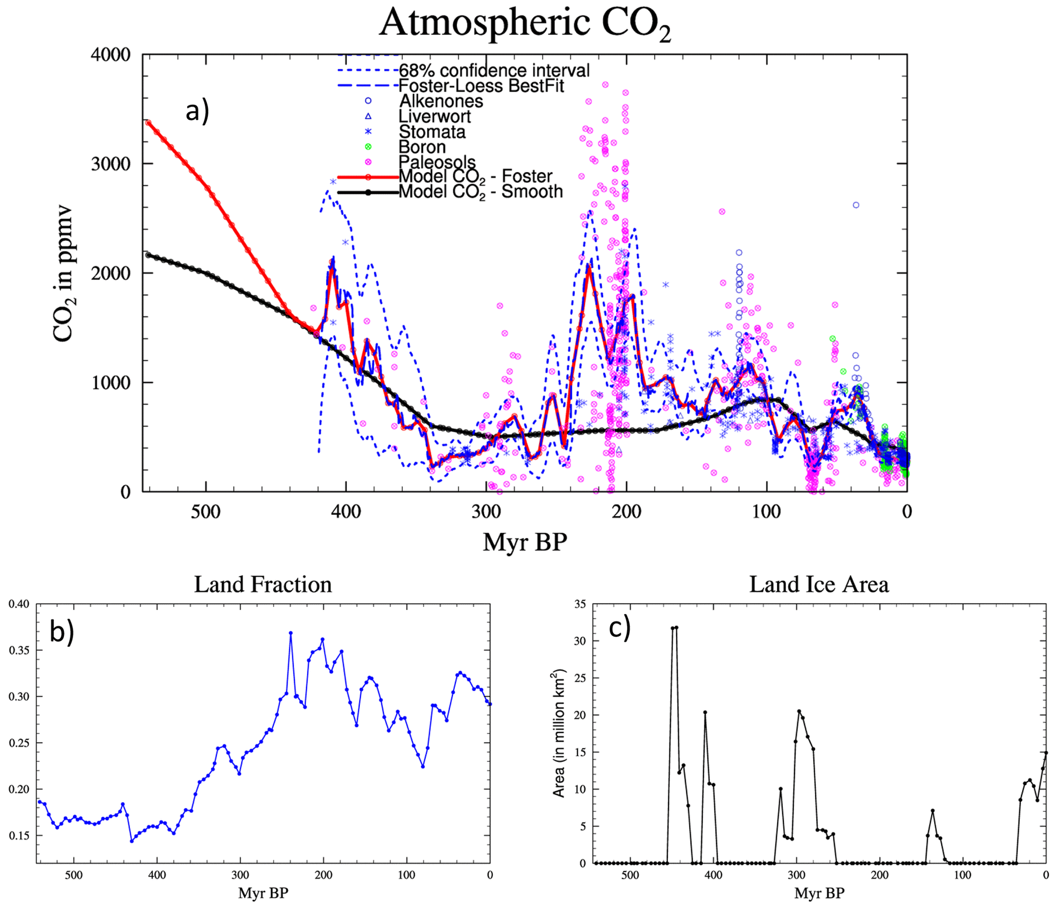
Figure 1Summary of boundary condition changes to model of the Phanerozoic, (a) CO2 reconstructions (from Foster et al., 2017) and the two scenarios used in the models, (b) land–sea fraction from the paleogeographic reconstructions, and (c) land ice area input into model. The paleogeographic reconstructions can be accessed at https://www.earthbyte.org/paleodem-resource-scotese-and-wright-2018/ (last access: 30 June 2021). An animation of the high-resolution () and model resolution (3.75∘ longitude × 2.5∘ latitude) maps can be found here: https://www.paleo.bristol.ac.uk/~ggpjv/scotese/scotese_raw_moll.normal_scotese_moll.normal.html (last access: 30 June 2021).
We refer to the simulation using the second set of CO2 reconstructions as the “smooth” CO2 simulations, though it should be recognized that the Foster CO2 curve has also been smoothed. The Foster CO2 curve extends back to only 420 Ma, so we have proposed two alternative extensions back to 540 Ma. Both curves increase sharply so that the combined forcing of CO2 and solar constant is approximately constant over this time period (Foster et al., 2017). The higher CO2 in the Foster curve relative to the “smooth” curve is because the initial set of simulations showed that the Cambrian simulations were relatively cool compared to data estimates for the period (Henkes et al., 2018).
2.3 Paleogeographic reconstructions
The 109 paleogeographic maps used in the HadleyCM3 simulations are digital representations of the maps in the PALEOMAP paleogeographic atlas (Scotese, 2016; Scotese and Wright, 2018). Table 1 lists all the time intervals that comprise the PALEOMAP paleogeographic atlas. The paleogeographic atlas contains one map for nearly every stage in the Phanerozoic. A paleogeographic map is defined as a map that shows the ancient configuration of the ocean basins and continents, as well as important topographic and bathymetric features such as mountains, lowlands, shallow sea, continental shelves, and deep oceans. Paleogeographic reconstructions older than the oldest ocean floor (∼ Late Jurassic) have uniform deep ocean floor depth.
Table 1List of paleogeographic maps and paleoDEMs.
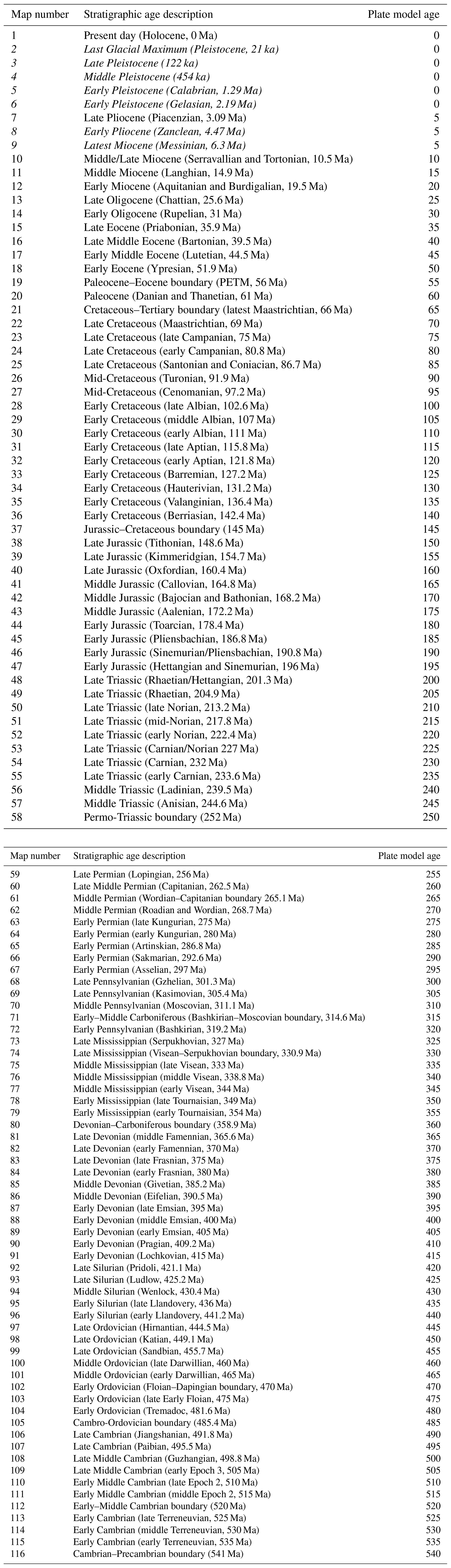
Simulations were not run for the time intervals highlighted in italics.
Once the paleogeography for each time interval has been mapped, this information is then converted into a digital representation of the paleotopography and paleobathymetry. Each digital paleogeographic model is composed of over 6 million grid cells that capture digital elevation information at a 10 km×10 km horizontal resolution and 40 m vertical resolution. This quantitative paleodigital elevation model, or “paleoDEM”, allows us to visualize and analyse the changing surface of the Earth through time using GIS software and other computer modelling techniques. For use with the HadCM3L climate model, the original high-resolution elevation grid was reduced to a () grid.
For a detailed description of how the paleogeographic maps and paleoDEMs were produced, the reader is referred to Scotese (2016), Scotese and Schettino (2017), and Scotese and Wright (2018). The work of Scotese and Schettino (2017) includes an annotated bibliography of the more-than-100 key sources of paleogeographic information. Similar paleogeographic paleoDEMs have been produced by Baatsen et al. (2016) and Verard et al. (2015).
The raw paleogeographic data reconstruct paleo-elevations and paleobathymetry at a resolution of . These data were re-gridded to resolution that matched the climate model using a simple area (for land–sea mask) or volume (for orography and bathymetry) conserving algorithm. The bathymetry was lightly smoothed (using a binomial filter) to ensure that the ocean properties in the resulting model simulations were numerically stable. This filter was applied multiple times in the high latitudes. The gridding sometimes produced single-grid-point enclosed ocean basins, particularly along complicated coastlines, and these were manually removed. Similarly, important ocean gateways were reviewed to ensure that the re-gridded coastlines preserved these structures. The resulting global fraction of land is summarized in Fig. 1b and examples are shown in Fig. 2. The original reconstructions can be found at https://www.earthbyte.org/paleodem-resource-scotese-and-wright-2018/ (last access: 30 June 2021). Maps of each HadCM3L paleogeography are included in the Supplement as figures.
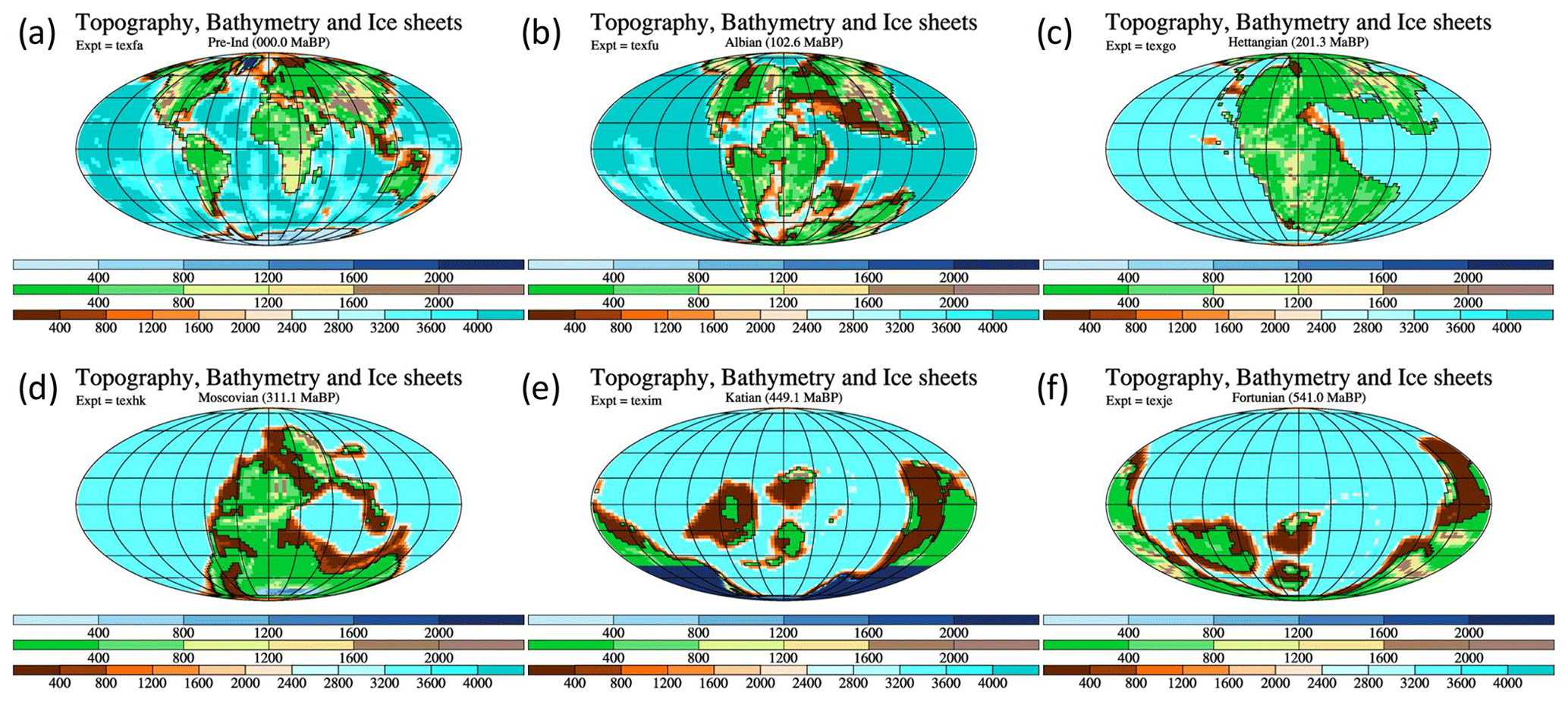
Figure 2A few example paleogeographies, once they have been re-gridded onto the HadCM3L grid. The examples are for (a) present day, (b) Albian, 102.6 Ma (Lower Cretaceous), (c) Hettangian, 201.3 Ma (lower Jurassic), (d) Moscovian, 311.1 Ma (Pennsylvanian, Carboniferous), (e) Katian, 449.1 Ma (Upper Ordovician), and (f) Fortunian, 541.0 Ma (Cambrian). The top colour legend refers to the height of the ice sheets (if they exist), the middle colour legend refers to heights on land (except ice), and the lower colour legend refers to the ocean bathymetry. All units are metres.
The paleogeographic reconstructions also include an estimate of land ice area (Scotese and Wright, 2018; Fig. 1c). These were converted to GCM boundary conditions assuming a simple parabolic shape to estimate the ice sheet height. These ice reconstructions suggest small amounts of land ice were present during the early Cretaceous, unlike Lunt et al. (2016), who used ice-free Cretaceous paleogeographies.
2.4 Spin-up methodology
The oceans are the slowest evolving part of the modelled climate system and can take multiple millennia to reach equilibrium, depending on the initial condition and climate state. To speed up the convergence of the model, we initialized the ocean temperatures and salinity with the values from previous model simulations from similar time periods using the commercial-in-confidence paleogeographies. Specifically, we had a set of 17 simulations covering the last 440 Myr. We selected the nearest simulation to the time period. For instance, the 10.5, 14.9, and the 19.5 Ma simulations were initialized from the 13 Ma simulation performed using the alternative paleogeographies. Table 2 summarizes the simulations performed in this study and shows the initialization of the model. The Foster CO2 simulations were initialized from the end point of the smooth CO2 simulations. In the first set of simulations (smooth CO2), we also attempted to accelerate the spin-up by using the ocean temperature trends at year 500 to linearly extrapolate the bottom 10 level temperatures for a further 1000 years. This had limited success and was not repeated. The atmosphere variables were also initialized from the previous model simulations but the spin-up of the atmosphere is much more rapid and did not require further intervention.
Table 2Summary of model simulations. The table summarizes the simulations performed in this study. The sixth and seventh columns refer to how the model was initialized. The smooth CO2 simulations were initialized from existing simulations using paleogeographies which were provided commercial in confidence. The time periods that these paleogeographies correspond to are listed in column 6, and the CO2 value used in the runs is in column 7. The Foster CO2 simulations were initialized from the end point of the smooth CO2 simulations.
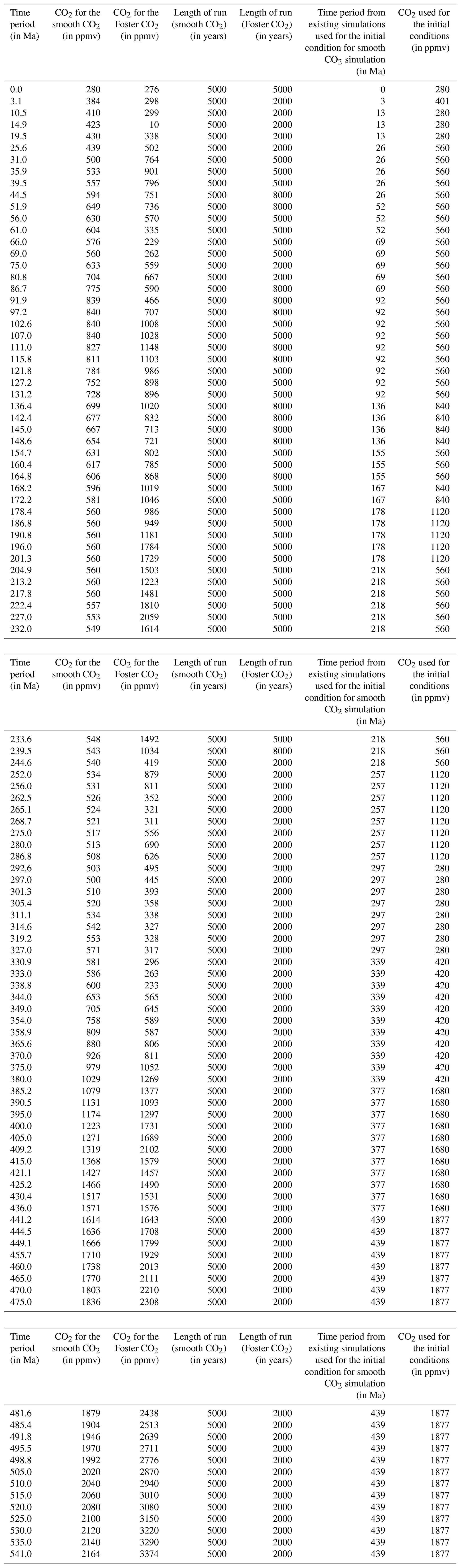
Simulations were run in parallel and thus were not initialized from the previous stage results using these paleogeographies. In total, we performed almost 1 million years of model simulation, and if we ran simulations in sequence, it would have taken 30 years to complete the simulations. By running these in parallel, initialized from previous modelling studies, we reduced the total runtime to 3 months, albeit using a substantial amount of our high-performance computer resources.
Although it is always possible that a different initialization procedure may produce different final states, it is impossible to explore the possibility of hysteresis/bistability without performing many simulations for each period, which is currently beyond our computing resources. Previous studies using HadCM3L (not published) with alternative ocean initial states (isothermals at 0, 8, and 16 ∘C) have not revealed multiple equilibria, but this might have been because we did not locate the appropriate part of parameter space that exhibits hysteresis. However, other studies have shown such behaviour (e.g. Baatsen et al., 2018). This remains a caveat of our current work and one which we wish to investigate when we have sufficient computing resources.
The simulations were then run until they reached equilibrium, as defined by the following:
-
The globally and volume-integrated annual mean ocean temperature trend is less than 1 ∘C per 1000 years, in most cases considerably smaller than this. We consider the volume-integrated temperature because it includes all aspects of the ocean. However, it is dominated by the deep ocean trends and is nearly identical to the trends at a depth of 2731 m (the lowest level that we have archived for the whole simulation).
-
The trends in surface air temperature are less than 0.3 ∘C per 1000 years.
-
The net energy balance at the top of the atmosphere, averaged over a 100-year period at the end of the simulation, is less than 0.25 W m−2 (in more than 80 % of the simulations, the imbalance is less than 0.1 W m−2). The Gregory plot (Gregory et al., 2004) implies surface temperatures are within 0.3 ∘C of the equilibrium state.
These target trends were chosen somewhat arbitrarily but are all less than typical orbital timescale variability (e.g. temperature changes since the last deglaciation were approximately 5 ∘C over 10 000 years). Most simulations were well within these criteria. In total, 70 % of simulations had residual net energy balances at the top of the atmosphere of less than 0.1 W m−2, but a few simulations were slower to reach full equilibrium. The strength of using multiple constraints is that a simulation may, by chance, pass one or two of these criteria but was unlikely to pass all three tests. For example, all the models that we extended failed at least two of the criteria. The resulting time series of volume-integrated global annual mean ocean temperatures are shown in Fig. 3. The figures in the Supplement also include this for each simulation, as well as the trends at 2731 m.
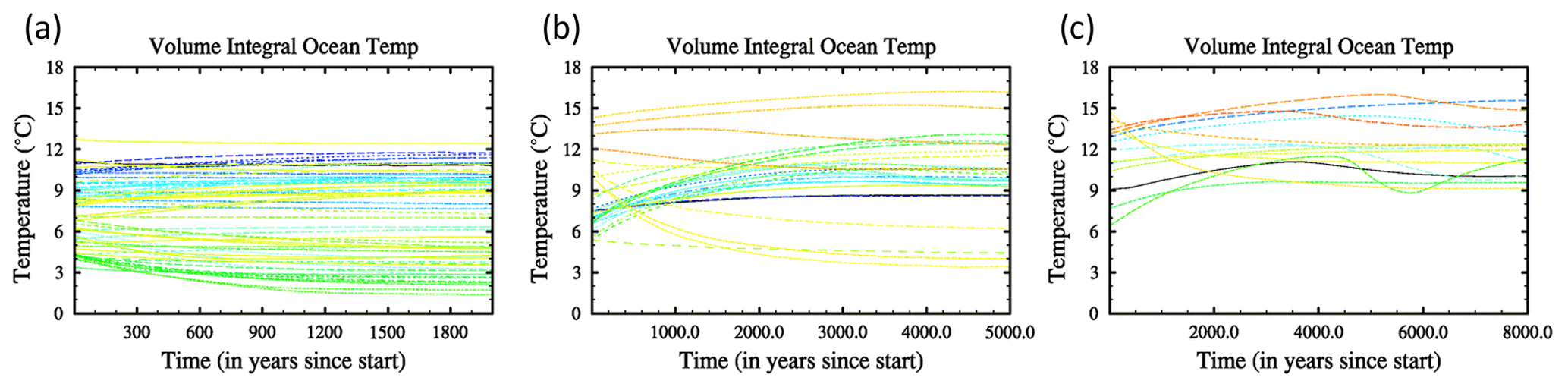
Figure 3Time series of the annual volume mean ocean temperature for all 109 simulations. Panel (a) shows those simulations for which 2000 years was sufficient to satisfy the convergence criteria described in the text (these were for all simulations listed in Table 1 except those listed in panels b and c), (b) those simulations which required 5000 years (these were for all the simulations for 31.0, 35.9, 39.5, 55.8, 60.6, 66.0, 69.0, 102.6, 107.0, 121.8, 127.2, 154.7, 160.4, 168.2, 172.2, 178.4, 186.8, 190.8, 196.0, 201.3, 204.9, 213.2, 217.8, 222.4, 227.0, 232.0, and 233.6 Ma), and (c) those simulation which required 8000 years (these were simulations for 44.5, 52.2, 86.7, 91.9, 97.2, 111.0, 115.8, 131.2, 136.4, 142.4, 145.0, 148.6, 164.8, and 239.5 Ma). The different coloured lines show the different runs. The plots simply show the extent to which all runs have reached steady state. For more details about specific simulations, please see the figures in the Supplement.
The “smooth” CO2 simulations were all run for 5050 model years and satisfied the criteria. The Foster CO2 simulations were initially run for a minimum of 2000 years (starting from the end of the 5000-year runs), at which point we reviewed the simulations relative to the convergence criteria. If the simulations had not converged, we extended the runs for an additional 3000 years. If they had not converged at the end of 5000 years, we extended them again for an additional 3000 years. After 8000 years, all simulations had converged based on the convergence criteria. In general, the slowest converging simulations corresponded to some of the warmest climates (final temperatures in Fig. 3b and c were generally warmer than those in Fig. 3a). It cannot be guaranteed that further changes will not occur; however, we note that the criteria and length of the simulations greatly exceed Paleoclimate Modelling Intercomparison Project – Last Glacial Maximum (PMIP-LGM) (Kageyama et al., 2017) and Deep-Time Model Intercomparison Project (PMIP-DeepMIP) (Lunt et al., 2017) protocols.
3.1 Comparison of deep ocean temperatures to benthic ocean data
Before using the model to investigate the linkage of deep ocean temperatures to global mean surface temperatures, it is interesting to evaluate whether the modelled deep ocean temperatures agree with the deep ocean temperatures obtained from the isotopic studies of benthic foraminifera (Zachos et al., 2008; Friedrich et al., 2012). It is important to note that the temperatures are strongly influenced by the choice of CO2, so we are not expecting complete agreement, but we simply wish to evaluate whether the model is within plausible ranges. If the modelled temperatures were in complete disagreement with data, then it might suggest that the model was too far away from reality to allow us to adequately discuss deep ocean–surface ocean linkages. If the modelled temperatures are plausible, then it shows that we are operating within the correct climate space. A detailed comparison of modelled surface and benthic temperatures to data throughout the Phanerozoic, using multiple CO2 scenarios, is the subject of a separate ongoing project.
Figure 4a compares the modelled deep ocean temperature to the foraminifera data from the Cenozoic and Cretaceous (115 Ma). The observed isotope data are converted to deep ocean temperature using the procedures described by Hansen et al. (2013). The modelled deep temperature shown in Fig. 4a (solid line) is the average temperature at the bottom level of the model, excluding depths less than 1000 m (to avoid continental shelf locations which are typically not included in benthic data compilations). The observed benthic data are collected from a range of depths and are rarely at the very deepest levels (e.g. the new cores in Friedrich et al. 2011 are from current water depths ranging from 1899 to 3192 m). Furthermore, large data compilations rarely include how the depth of a particular site changed with time, and thus effectively assume that any differences between basins and through time are entirely due to climate change and not to changes in depth. Hence, throughout the rest of the paper, we frequently use the modelled 2731 m temperatures as a surrogate for the true benthic temperature. This is a pragmatic definition because the area of deep ocean reduces rapidly (e.g. there is typically only 50 % of the globe deeper than 3300 m). To evaluate whether this procedure gave a reasonable result, we also calculated the global average temperature at the model bottom and at the model level at a depth of 2731 m. The latter is shown by the dashed line in Fig. 4a. In general, the agreement between model bottom water temperatures and 2731 m temperatures is very good. The standard deviation between model bottom water and constant depth of 2731 m is 0.7 ∘C, and the maximum difference is 1.4 ∘C. Compared to the overall variability, this is a relatively small difference and shows that it is reasonable to assume that the deep ocean has weak vertical gradients.
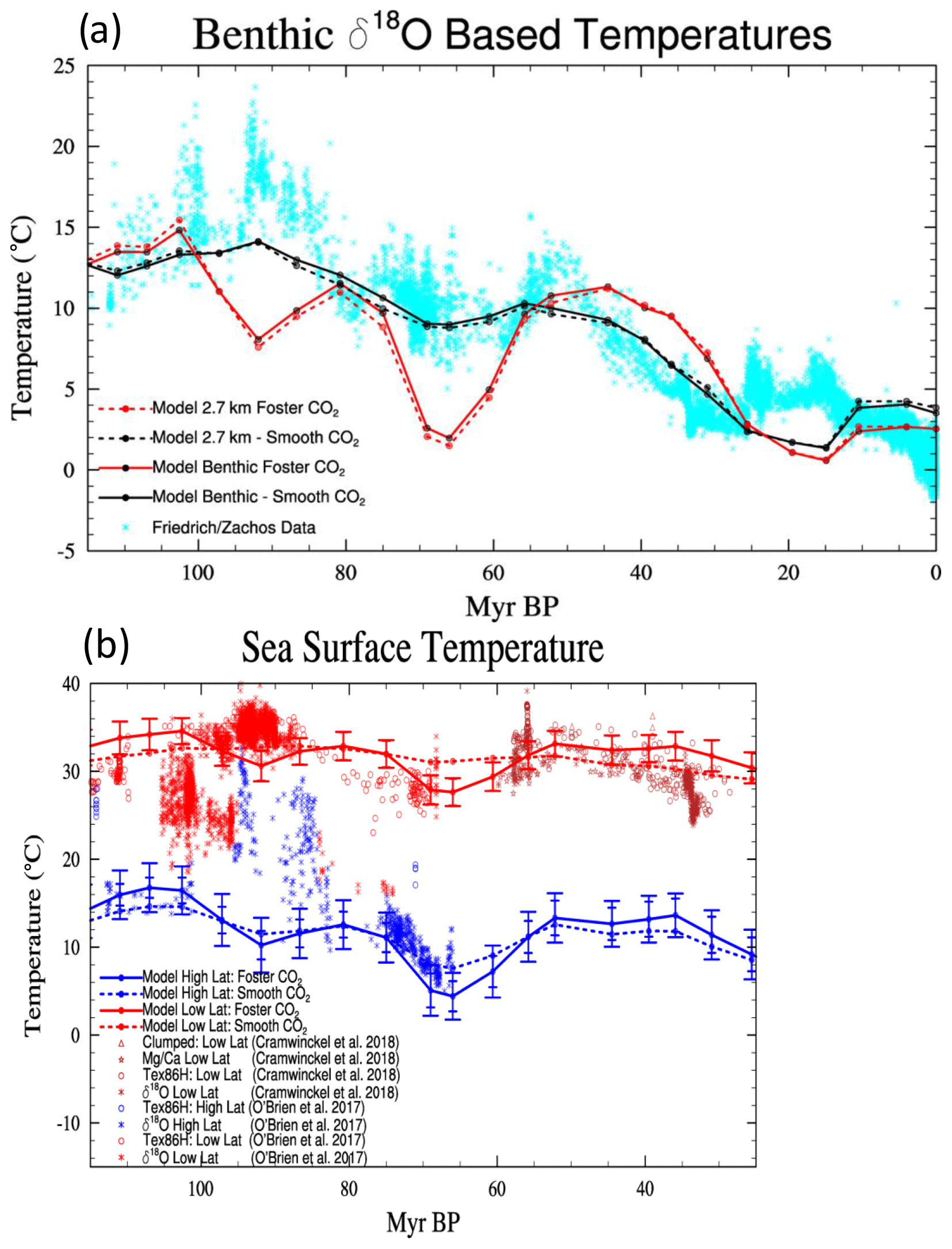
Figure 4(a) Comparison of modelled deep ocean temperatures versus those from Zachos et al. (2008) and Friedrich et al. (2012) converted to temperature using the formulation in Hansen et al. (2013). The model temperatures are global averages over the bottom layer of the model but exclude shallow marine settings (less than 1000 m). The dashed lines show the modelled global average ocean temperatures at the model layer centred at 2731 m and (b) comparison of modelled sea surface temperatures with the compilations of O'Brien et al. (2017) and Cramwinckel et al. (2018). The data are a combination of Tex86, δ18O, , and clumped isotope data. The model data show low-latitude temperatures (averaged from 10∘ S to 10∘ N) and high-latitude temperatures (averaged over 47.5 to 65∘ N and 47.5 to 65∘ S). The Foster CO2 simulations also show a measure of the spatial variability. The large bars show the spatial standard deviation across the whole region, and the smaller bars show the average spatial standard deviation along longitudes within the region. Note that the ranges of both the x and y axes differ between panels (a) and (b).
The total change in benthic temperatures over the Late Cretaceous and Cenozoic is well reproduced by the model, with the temperatures associated with the “smooth” CO2 record being particularly good. We do not expect the model to represent substage changes (hundreds of thousands of years) such as the Paleocene-Eocene Thermal Maximum excursion or ocean anoxic events, but we do expect that the broader temperature patterns should be simulated.
Comparison of the two simulations illustrates how strongly CO2 controls global mean temperature. The Foster-CO2-driven simulation substantially differs from the estimates of deep-sea temperature obtained from benthic foraminifera and is generally a poorer fit to data. The greatest mismatch between the Foster curve and the benthic temperature curve is during the Late Cretaceous and early Paleogene. Both dips in the Foster CO2 simulations correspond to relatively low estimates of CO2 concentrations. For these periods, the dominant source of CO2 values is from paleosols (Fig. 1), and thus we are reliant on one proxy methodology. Unfortunately, the alternative CO2 reconstructions of Witkowski et al. (2018) have a data gap during these periods.
A second big difference between the Foster curve and the benthic temperature curve occurs during the Cenomanian–Turonian. This difference is similarly driven by a low estimate of CO2 in the Foster CO2 curve. These low CO2 values are primarily based on stomatal density indices. As can be seen in Fig. 1, stomatal indices frequently suggest CO2 levels lower than estimates obtained by other methods. The CO2 estimates by Witkowski et al. (2018) generally supports the higher levels of CO2 (near 1000 ppmv) that are suggested by the “smooth” CO2 curve.
Both sets of simulations underestimate the warming during the middle Miocene. This issue has been seen before in other models, e.g. You et al. (2009), Knorr et al. (2011), Krapp and Jungclaus (2011), Goldner et al. (2014), and Steinthorsdottir et al. (2021). In order to simulate the surface warmth of the middle Miocene (15 Ma), CO2 concentrations in the range 460–580 ppmv were required, whereas the CO2 reconstructions for this period (Foster et al., 2017) are generally quite low (250–400 ppmv). This problem may be either due to the climate models having too low a climate sensitivity or that the estimates of CO2 are too low (Stoll et al., 2019).
The original compilation of Zachos et al. (2008) represented a relatively small portion of the global ocean, and the implicit assumption was made that these results represented the entire ocean basin. Cramer et al. (2009) examined the data from an ocean basin perspective and suggested that these inter-basin differences were generally small during the Late Cretaceous and early Paleogene (90–35 Ma), and the differences between ocean basins were larger during the late Paleogene and early Neogene. Our model largely also reproduces this pattern. Figure 5 shows the ocean temperature at 2731 m during the Late Cretaceous (69 Ma), the late Eocene (39 Ma), and the Oligocene (31 Ma) for the “smooth” CO2 simulations. In the Late Cretaceous, the model temperatures are almost identical in the North Atlantic and Pacific (8–10 ∘C). There is warmer deep water forming in the Indian Ocean (deep mixed layer depths; not shown) and off the west coast of Australia (10–12 ∘C), but otherwise the pattern is very homogeneous. This is in agreement with some paleoreconstructions for the Cretaceous (e.g. Murphy and Thomas, 2012).
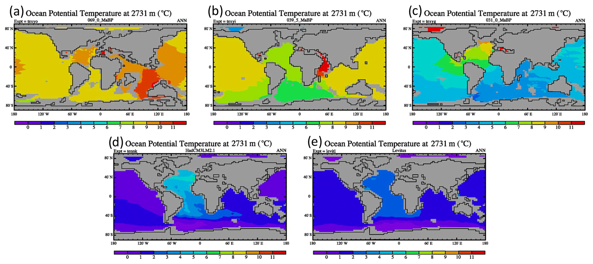
Figure 5Modelled annual mean ocean temperatures at 2731 m depth for three examples of past time periods. Panel (a) is for the Late Cretaceous, panel (b) is for the late Eocene (39.5 Ma), and panel (c) is for the Oligocene (31 Ma). These are results from the smooth CO2 set of simulations which agree better with the observed benthic temperature data. Also included are (d) the pre-industrial simulations and (e) the World Ocean Atlas 1994 observational data, provided by the NOAA-ESRL Physical Sciences Laboratory, Boulder, Colorado, from their website at https://psl.noaa.gov/ (last access: 30 June 2021). The thin black lines show the coastlines, and the grey areas are showing where the ocean is shallower than 2731 m.
By the time we reach the late Eocene (39 Ma), the North Atlantic and Pacific remain very similar but cooler deep water (6–8 ∘C) is now originating in the South Atlantic. The South Atlantic cool bottom water source remains in the Oligocene, but we see a strong transition in the North Atlantic to an essentially modern circulation with the major source of deep, cold water occurring in the high southerly latitudes (3–5 ∘C) and strong gradient between the North Atlantic and Pacific.
Figure 5 also shows the modelled deep ocean temperatures for the present day (Fig. 5d) compared to the World Ocean Atlas data (Fig. 5e). It can be seen that the broad patterns are well reproduced in the model, with good predictions of the mean temperature of the Pacific. The model is somewhat too warm in the Atlantic itself and has a stronger plume from the Mediterranean than is shown in the observations.
3.2 Comparison of model sea surface temperature to proxy data
The previous section focused on benthic temperatures, but it is also important to evaluate whether the modelled sea surface temperatures are plausible (within the uncertainties of the CO2 reconstructions). Figure 4b shows a comparison between the model simulations of sea surface temperature and two published syntheses of proxy SST data. O'Brien et al. (2017) compiled TEX86 and δ18O for the Cretaceous, separated into tropical and high-latitude (polewards of 48∘) regions. Cramwinckel et al. (2018) compiled early Cenozoic tropical SST data, using Tex86, δ18O, , and clumped isotopes. We compare these to modelled SST for the region 15∘ S to 15∘ N and for the average of the Northern Hemisphere and Southern Hemisphere between 47.5 and 60∘N/S. The proxy data include sites from all ocean basins and so we also examined the spatial variability within the model. This spatial variability consists of changes along longitude (effectively different ocean basins) and changes with latitude (related to the gradient between the Equator and the poles). We therefore calculated the average standard deviation of SST relative to the zonal mean at each latitude (this is shown by the smaller tick marks) and the total standard deviation of SST relative to the regional average. In practice, the equatorial values are dominated by inter-basin variations, and hence the two measures of spatial variability are almost identical. The high-latitude variability has a bigger difference between the longitudinal variations and the total variability, because the Equator-to-pole temperature gradient (i.e. the temperatures at the latitude limits of the region) is a few degrees warmer or colder than the average. The spatial variability was very similar for the smooth CO2 and Foster CO2 simulations, so for clarity, in Fig. 4b, we only show the results as error bars on the model Foster CO2 simulations.
Overall, the comparison between model and data is generally reasonable. The modelled equatorial temperatures largely follow the data, albeit with considerable scatter in the data. Both simulations tend to be towards the warmest equatorial data in the early Cretaceous (Albian). These temperatures largely come from Tex86 data. There are many δ18O-based SSTs which are significantly colder during this period. These data almost exclusively come from cores 1050/1052, which are in the Gulf of Mexico. It is possible that these data are offset due to a bias in the δ18O of sea water because of the relatively enclosed region. The Foster CO2 simulations are noticeably colder than the data at the Cenomanian peak warmth, which is presumably related to the relatively low CO2, as discussed for the benthic temperatures. The benthic record also showed a cool (low CO2) bias in the Late Cretaceous. This is not such an obvious feature of the surface temperatures. The Foster simulations are colder than the smooth CO2 simulations during the Late Cretaceous but there is not a strong mismatch between model and data. Both simulations are close to the observations, though the smooth CO2 simulations better match the high-latitude data (but show slightly poorer match with the tropical data).
The biggest area of disagreement between model and data is at high latitudes in the mid-Cretaceous warm period. In common with previous work with this model in the context of the Eocene (Lunt et al., 2021), the model is considerably cooler than the data, with a 10–15 ∘C mismatch between models and data. The polar sea surface temperature estimates may have a seasonal bias because productivity is likely to be higher during the warmer summer months, and, if we select the summer season temperatures from the model, then the mismatch is slightly reduced by about 4 ∘C. The problem of cool high latitudes in models is seen in many model studies, and there is increasing evidence that this is related to the way that the models simulate clouds (Kiehl and Shields, 2013; Sagoo et al., 2013; Zhu et al., 2019; Upchurch et al., 2015). Of course, in practice, deep water is formed during winter so the benthic temperatures do not suffer from a summer bias.
3.3 Correlation of deep ocean temperatures to polar sea surface temperatures
The previous sections showed that the climate model was producing a plausible reconstruction of past ocean temperature changes, at least within the uncertainties of the CO2 estimates. We now use the HadCM3L model to investigate the links between deep ocean temperature and global mean surface temperature.
In theory, the deep ocean temperature should be correlated with the sea surface temperature at the location of deep-water formation which is normally assumed to be high-latitude surface waters in winter. We therefore compare deep ocean temperatures (defined as the average temperature at the bottom of the model ocean, where the bottom must be deeper than 1000 m) with the average winter sea surface temperature polewards of 60∘ (Fig. 6). Winter is defined as December, January, and February (DJF) in the Northern Hemisphere and June, July, and August (JJA) in the Southern Hemisphere. Also shown in Fig. 6 is the best-fit line, which has a slope of 0.40 (±0.05 at the 97.5 % level), an r2 of 0.59, and a standard error of 1.2 ∘C. We obtained very similar results when we compared the polar sea surface temperatures with the average temperature at 2731 m instead of the true benthic temperatures. We also compared the deep ocean temperatures to the mean polar sea surface temperatures when the mixed layer depth exceeded 250 m (poleward of 50∘N/S). The results were similar, although the scatter was somewhat larger (r2=0.48).
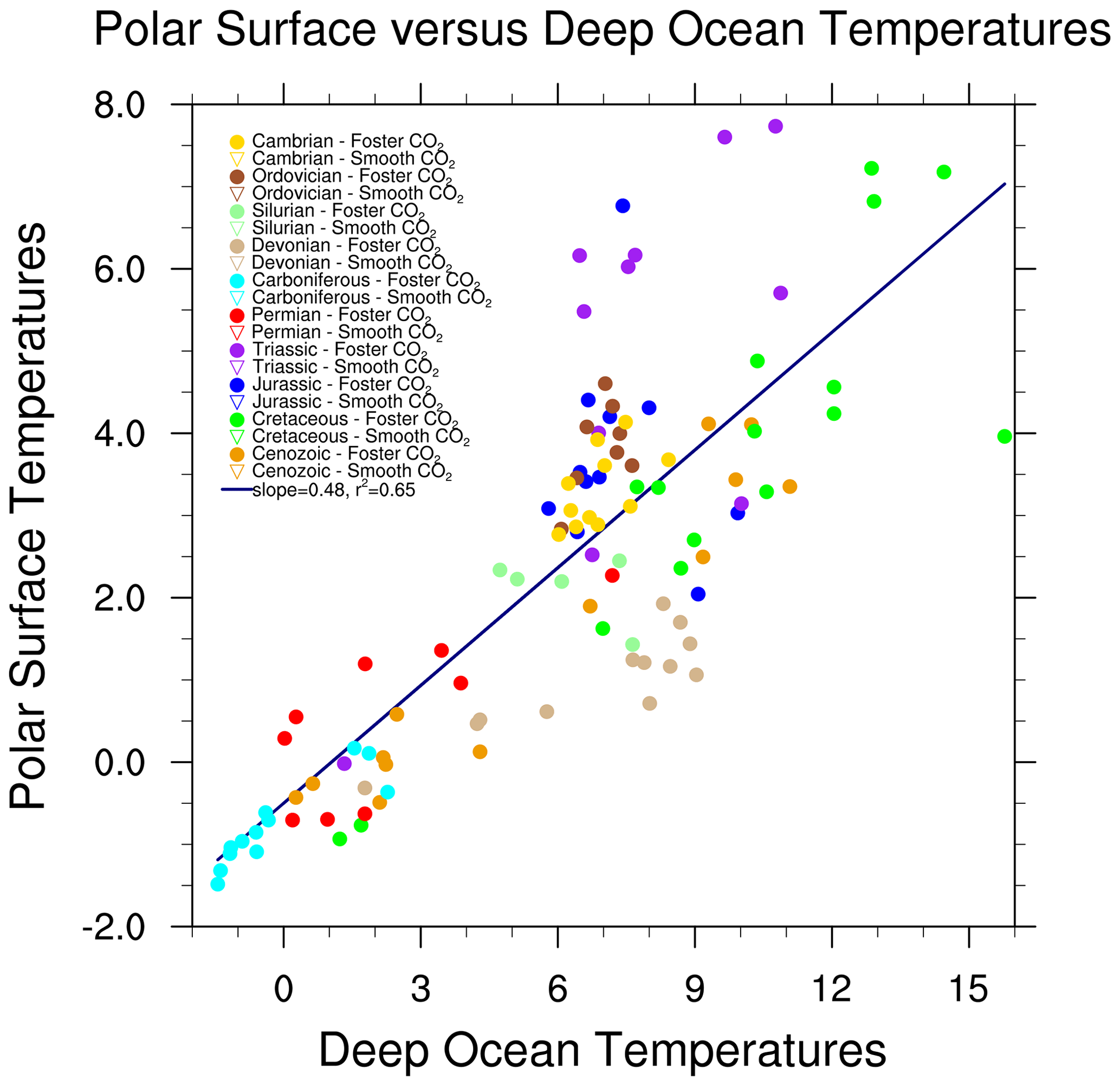
Figure 6Correlations between deep ocean temperatures and surface polar sea surface temperatures. The deep ocean temperatures are defined as the average temperature at the bottom of the model ocean, where the bottom must be deeper than 1000 m. The polar sea surface temperatures are the average winter (i.e. northern polar in DJF and southern polar in JJA) sea surface temperature polewards of 60∘. The inverted triangles show the results from the smooth CO2 simulations and the dots refer to the Foster CO2 simulations. The colours refer to different geological eras.
Overall, the relationship between deep ocean temperatures and polar sea surface temperatures is clear (Fig. 6) but there is considerable scatter around the best-fit line, especially at the high end, and the slope is less steep than perhaps would be expected (Hansen and Sato, 2012). The scatter is less for the Cenozoic and Late Cretaceous (up to 100 Ma: green and orange dots and triangles). If we used only Cenozoic and Late Cretaceous simulations, then the slope is similar (0.43) but with r2=0.92 and a standard error of 0.47 ∘C. This provides strong confirmation that benthic data are a robust approximation to polar surface temperatures when the continental configuration is similar to the present.
However, the scatter is greater for older time periods, with the largest divergence observed for the warm periods of the Triassic and early Jurassic, particularly for the Foster CO2 simulations (purple and blue dots). Examination of climate models for these time periods reveals relatively sluggish and shallow ocean circulation, with weak horizontal temperature gradients at depth (though salinity gradients can still be important; Zhou et al., 2008). For instance, in the Ladinian, mid-Triassic stage (∼240 Ma), the overturning circulation is extremely weak (Fig. 7). The maximum strength of the Northern Hemisphere overturning cell is less than 10 Sv and the southern cell is less than 5 Sv. Under these conditions, deep ocean water does not always form at polar latitudes. Examination of the mixed layer depth (not shown) shows that during these time periods, the deepest mixed layer depths are in the subtropics. In subtropics, there is very high evaporation relative to precipitation (due to the low precipitation and high temperatures). This produces highly saline waters that sink and spread out into the global ocean.
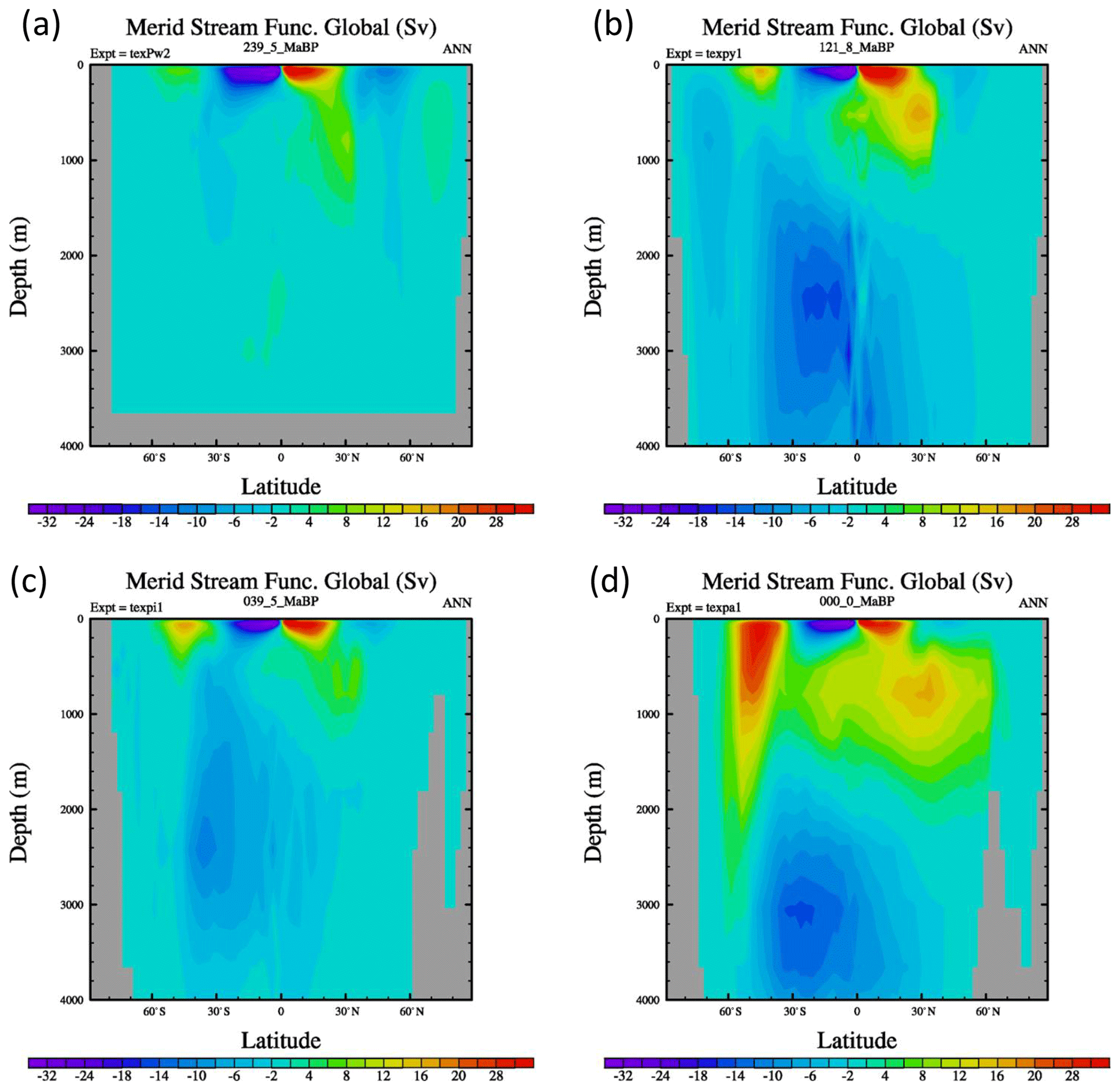
Figure 7Global ocean overturning circulation (in Sverdrups) for four different time periods for the Foster CO2 simulations. Positive (yellow/red) values correspond to a clockwise circulation; negative (dark blue/purple) values represent an anti-clockwise circulation. (a) Middle Triassic, Ladinian, 239.5 Ma, (b) Lower Cretaceous, Aptian, 121.8 Ma, (c) Late Eocene, Bartonian, 39.5 Ma, and (d) present day. Paleogeographic reconstructions older than the oldest ocean floor (∼ Late Jurassic) have uniform deep ocean floor depth.
The idea that deep water may form in the tropics is in disagreement with early hypotheses (e.g. Emiliani, 1954), but they were only considering the Tertiary, and our model does not simulate any low-latitude deep-water formation during this period. We only see significant tropical deep-water formation for earlier periods, and this has previously been suggested as a mechanism for warm Cretaceous deep-water formation (Brass et al., 1982; Kennett and Stott, 1991). Deep water typically forms in convective plumes. Brass et al. (1982) showed that the depth and spreading of these plumes are related to the buoyancy flux, with the greatest flux leading to bottom water and plumes of lesser flux leading to intermediate water. Brass et al. (1982) suggested that this could occur in warm conditions in the tropics, particularly if there were significant epicontinental seaways, and hypothesized that it “has been a dominant mechanism of deep-water formation in historical times”. It is caused by a strong buoyancy flux linked to strong evaporation at high temperatures.
Our computer model simulations are partly consistent with this hypothesis. The key aspect for the model is a relatively enclosed seaway in the tropics and warm conditions. The paleogeographic reconstructions (see figures in the Supplement) suggest an enclosed Tethyan-like seaway starting in the Carboniferous and extending through to the Jurassic and early Cretaceous. However, the colder condition of the Carboniferous prevents strong tropical buoyancy fluxes. When we get into the Triassic and Jurassic, the warmer conditions lead to strong evaporation at low latitudes and bottom water formation in the tropics. This also explains why we see more tropical deep water (and hence poorer correlations between deep and polar surface temperatures in Fig. 6) when using the Foster CO2 since this is generally higher (and hence warmer) than the smoothed CO2 record.
An example of the formation of tropical deep water is shown in Fig. 8. This shows a vertical cross section of temperature and salinity near the Equator for the Ladinian stage, mid-Triassic (240 Ma). The salinity and temperature cross section clearly shows high-salinity warm waters sinking to the bottom of the ocean and spreading out. This is further confirmed by the water age tracer in Fig. 9. This shows the water age (measured as time since it experienced surface conditions; see England, 1995) at 2731 m in the model for the Permian, Triassic, Cretaceous, and the present day. The present-day simulation shows that the youngest water is in the North Atlantic and off the coast of Antarctica, indicating that this is where the deep water is forming. By contrast, the Triassic period shows that the youngest water is in the tropical Tethyan region and that it spreads out from there to fill the rest of the ocean basin. There is no young water at high latitudes, confirming that the source of bottom water is tropical only. For the Permian, although there continues to be a Tethyan-like tropical seaway, the colder conditions mean that deep water is again forming at high latitudes only. The Cretaceous is more complicated. It shows younger water in the high latitudes, but also shows some young water in the Tethys which merges with the high-latitude waters. An additional indicator of the transitional nature of the Cretaceous is the mixed layer depth (see figures in the Supplement). This is a measure of where water is mixing to deeper levels. For this time period, there are regions of deep mixed layer in both the tropics and high latitudes, whereas it is only deep in the tropics for the Triassic and at high latitudes for the present day.
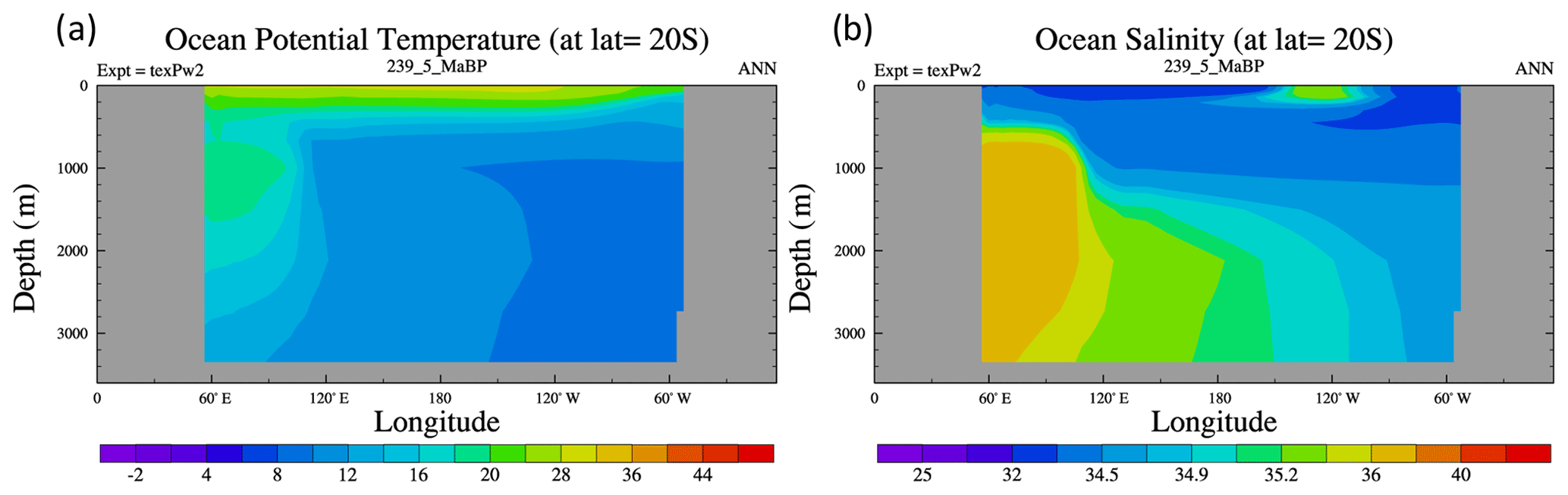
Figure 8Longitudinal cross section at 20∘S of (a) ocean potential temperature and (b) salinity for the Ladinian (240 Ma). Temperature is in Celsius and salinity is in PSU.
This mechanism for warm deep-water formation has also been seen in other climate models (e.g. Barron and Peterson, 1990). However, Poulsen et al. (2001) conclude that in their model of the Cretaceous, high-latitude sources of deep water diminish with elevated CO2 concentrations but did not see the dominance of tropical sources. Other models (e.g. Ladant et al., 2020) do not show any significant tropical deep-water formation, suggesting that this feature is potentially a model-dependent result.
The correlation between deep ocean temperatures and the temperature of polar surface waters differs between the “smooth” CO2 simulations and the Foster CO2 simulations. The slope is only 0.30 (r2=0.57) for the “smooth” CO2 simulations, whereas the slope is 0.48 (r2=0.65) for the Foster simulations. This is because CO2 is a strong forcing agent that influences both the surface and deep ocean temperatures. By contrast, if the CO2 does not vary as much, then the temperature does not vary as much, and the influence of paleogeography becomes more important. These paleogeographic changes generally cause subtle and complicated changes in ocean circulation that affect the location and latitude of deep-water formation.
In contrast, the mid-Cretaceous is also very warm but the continental configuration (specifically, land at high southern latitudes) favours the formation of cool, high-latitude deep water. Throughout the Cretaceous, there is a significant southern high-latitude source of deep water, and hence deep-water temperatures are well correlated with surface high-latitude temperatures. The strength of this connection, however, may be overexaggerated in the model. Like many climate models, HadCM3 underestimates the reduction in the pole-to-Equator sea surface temperature (Lunt et al., 2012, 2021). This means that during the Cretaceous the high latitudes are probably too cold. Consequently, some seasonal sea ice does form, which encourages the formation of cold deep water, via brine rejection.
In the late Eocene (∼40 Ma), the ocean circulation is similar to the Cretaceous, but the strong southern overturning cell is closer to the South Pole, indicating that the main source of deep water has moved further polewards. The poleward movement of the region of downwelling waters explains some of the variability between deep ocean temperatures and temperature of polar surface waters.
For reference, we also include the present-day meridional circulation. The modern Southern Hemisphere circulation is essentially a strengthening of late Eocene meridional circulation. The Northern Hemisphere is dominated by the Atlantic meridional overturning circulation. The Atlantic circulation pattern does not resemble the modern pattern of circulation until the Miocene.
3.4 Surface polar amplification
The conceptual model used to connect benthic ocean temperatures to global mean surface temperatures assumes that there is a constant relationship between high-latitude sea surface temperatures and global mean annual mean surface air temperature. Hansen and Sato (2012) argue that this amplification is partly related to ice–albedo feedback but also includes a factor related to the contrasting amplification of temperatures on land compared to the ocean. To investigate the stability of this relationship, Fig. 10 shows the correlation between polar winter sea surface temperatures (between 60 and 90∘ in both hemispheres) and global mean surface air temperature. The polar temperatures are the average of the two winter hemispheres (i.e. average of DJF polar SSTs in the Northern Hemisphere and JJA polar SSTs in the Southern Hemisphere). Also shown is a simple linear regression, with an average slope of 1.3 and with r2=0.79. If we only use northern polar winter temperatures, the slope is 1.1; if we only use southern polar winter temperatures, then the slope is 0.7. Taken separately, the scatter about the mean is considerably larger (r2 of 0.5 and 0.6, respectively) than the scatter if both datasets are combined (r2=0.79). The difference between the Southern Hemisphere and Northern Hemisphere response complicates the interpretation of the proxies and leads to potentially substantial uncertainties.
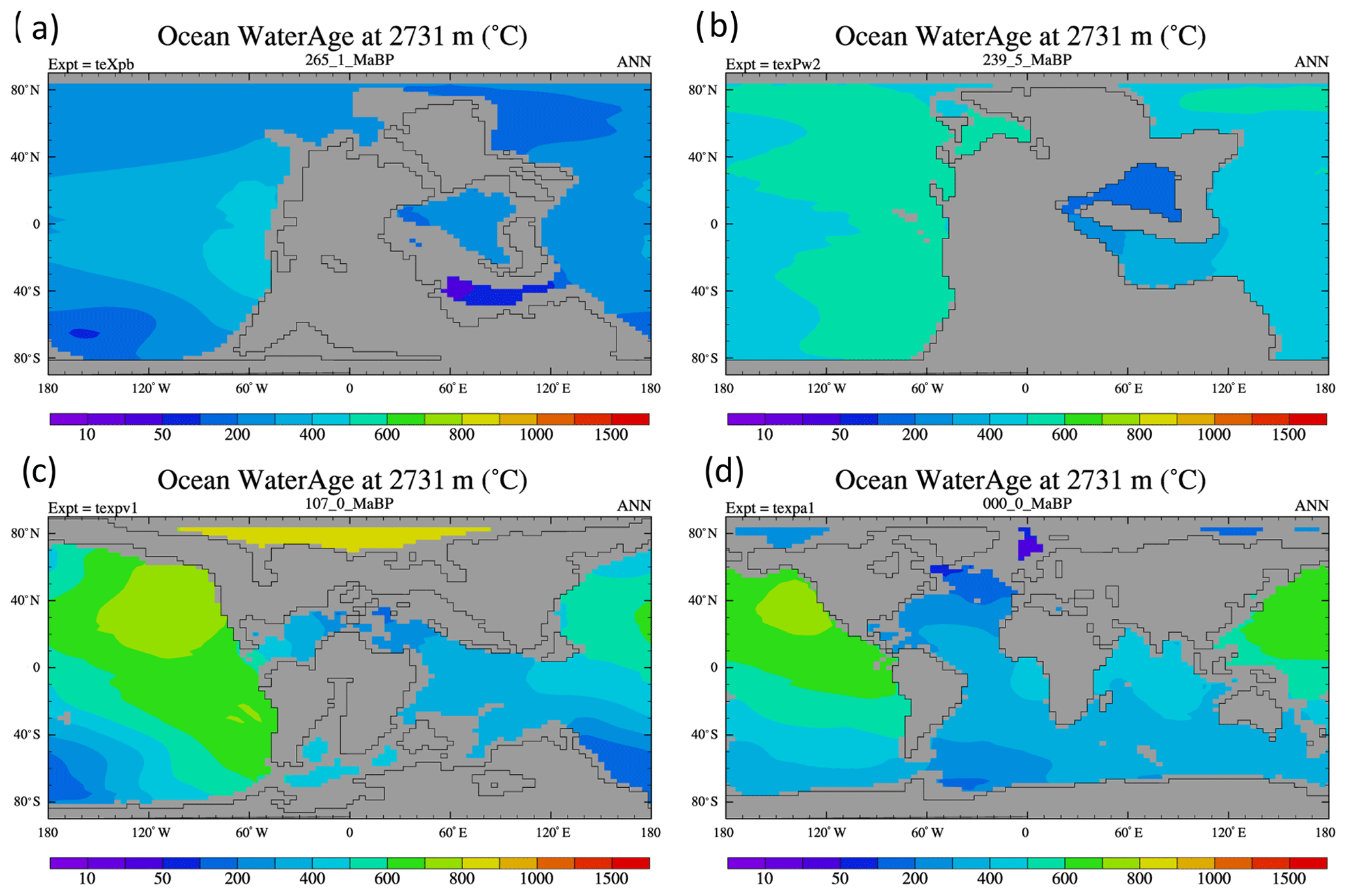
Figure 9Modelled age of water tracer at 2731 m for four different time periods: (a) 265 Ma, (b) 240 Ma, (c) 107 Ma, and (d) 0 Ma. Units are years.
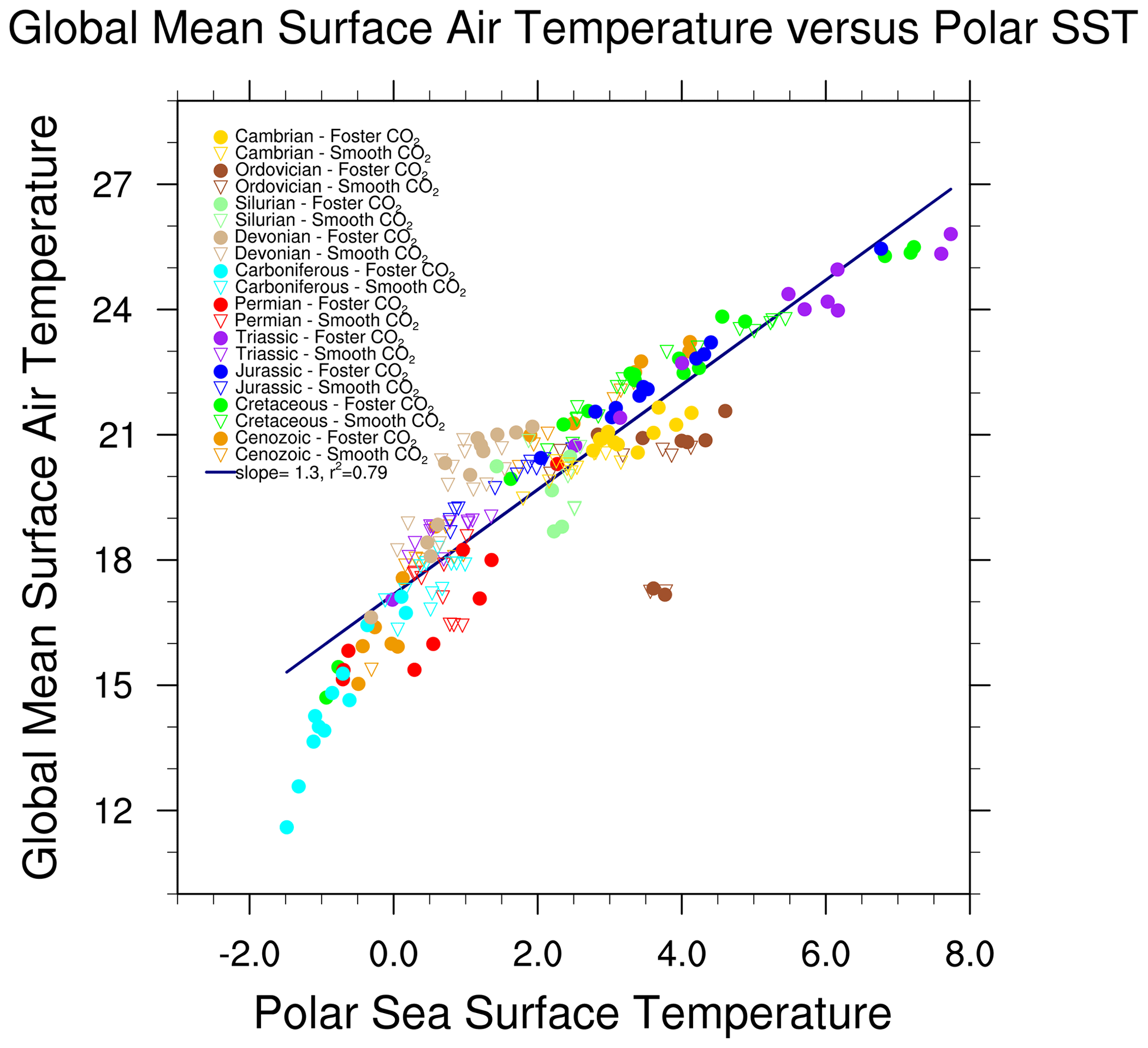
Figure 10Correlation between high-latitude ocean temperatures (polewards of 60∘) and the annual mean, global mean surface air temperature. The polar temperatures are the average of the two winter hemispheres (i.e. northern DJF and southern JJA). Other details are as in Fig. 6.
As expected, there appears to be a strong non-linear component to the correlation. There are two separate regimes: (1) one with a steeper slope during colder periods (average polar winter temperature less than about 1 ∘C) and (2) a shallower slope for warmer conditions. This is strongly linked to the extent of sea-ice cover. Cooler periods promote the growth of sea ice which strengthens the ice–albedo feedback mechanism, resulting in a steeper overall temperature gradient (strong polar amplification). Of course, the ocean sea surface temperatures are constrained to be −2 ∘C but an expansion of sea ice moves this further equatorward. Conversely, the warmer conditions result in less sea ice and hence a weaker sea ice–albedo feedback, resulting in a weaker temperature gradient (reduced polar amplification). This suggests that using a simple linear relationship (as in Hansen et al., 2008) could be improved upon.
Examining the Foster CO2 and “smooth” CO2 simulations reveals an additional factor. If we examine the smooth CO2 simulations only, then the best-fit linear slope is slightly less than the average slope (1.1 versus 1.3). This can be explained by the fact that we have fewer very cold climates (particularly in the Carboniferous) due to the relatively elevated levels of CO2. However, the scatter in the “smooth” CO2 correlation is much larger, with an r2 of only 0.66. By comparison, correlation between global mean surface temperature and polar sea surface temperature using the Foster CO2 has a similar overall slope to the combined set and a smaller amount of scatter. This suggests that CO2 forcing and the polar amplification response have an important impact on the relationship between global and polar temperatures. The variations of carbon dioxide in the Foster set of simulations are large and they drive large changes in global mean temperature. Conversely, significant sea-ice–albedo feedbacks characterize times when the polar amplification is important. There are several well-studied processes that lead to such changes, including albedo effects from changing ice but also from poleward heat transport changes, cloud cover, and latent heat effects (Sutton et al., 2007; Alexeev et al., 2005; Holland and Bitz, 2003). By contrast, the smooth CO2 simulations have considerably less forcing due to CO2 variability, which leads to a larger paleogeographic effect. For instance, when there is more land at the poles, there will be more evaporation over the land areas, and hence simple surface energy balance arguments would suggest different temperatures (Sutton et al., 2007).
In Fig. 10, there are a few data points which are complete outliers. These correspond to simulations in the Ordovician; the outliers happen irrespective of the CO2 model that is used. Inspection of these simulations shows that the cause for this discrepancy is related to two factors: (1) a continental configuration with almost no land in the Northern Hemisphere and (2) a reconstruction which includes significant Southern Hemisphere ice cover (see Figs. 1 and 2). Combined, these factors produced a temperature structure which is highly non-symmetric, with the southern high latitudes being more than 20 ∘C colder than the northern high latitudes. This anomaly biases the average polar temperatures shown in Fig. 10.
3.5 Deep ocean temperature versus global mean temperature
The relationships described above help to understand the overall relationship between deep ocean temperatures and global mean temperature. Figure 11 shows the correlation between modelled deep ocean temperatures (>1000 m) and global mean surface air temperature, and Fig. 12 shows a comparison of changes in modelled deep ocean temperature compared to model global mean temperature throughout the Phanerozoic.
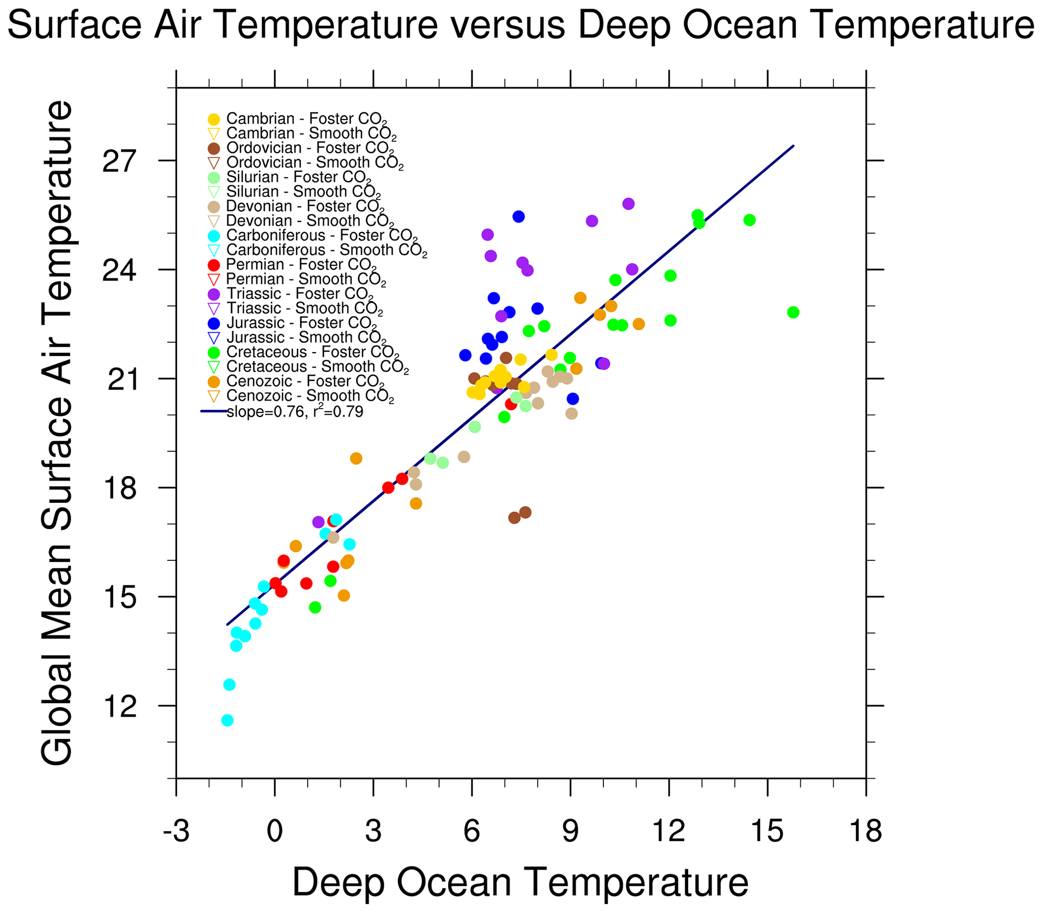
Figure 11Correlation between the global mean, annual mean surface air temperature and the deep ocean temperature. The deep ocean temperatures are defined as the average temperature at the bottom of the model ocean, where the bottom must be deeper than 1000 m. Other details are as in Fig. 6.
The overall slope is 0.64 (0.59 to 0.69) with r2=0.74. If we consider the last 115 Myr (for which there exist compiled benthic temperatures), then the slope is slightly steeper (0.67 with an r2=0.90). Similarly, the smooth CO2 and the Foster CO2 simulation results have very different slopes. The smooth CO2 simulations have a slope of 0.47, whereas the Foster CO2 simulations have a slope of 0.76. The root mean square departure from the regression line in Fig. 11 is 1.3 ∘C. Although we could have used a non-linear fit as we might expect such a relationship if the pole-to-Equator temperature gradient changes, all use of benthic temperatures as a global mean surface temperature proxy is based on a linear relationship.
The relatively good correlations in Fig. 11 are confirmed when examining Fig. 12a and b. On average, the deep ocean temperatures tend to underestimate the global mean change (Fig. 12b), which is consistent with the regression slope being less than 1. However, the errors are substantial, with the largest errors occurring during the pre-Cretaceous, and can be 4–6 ∘C. This is an appreciable error that would have a substantial impact on estimates of climate sensitivity. Even within the Late Cretaceous and Cenozoic, the errors can exceed 2 ∘C, which can exceed 40 % of the total change.
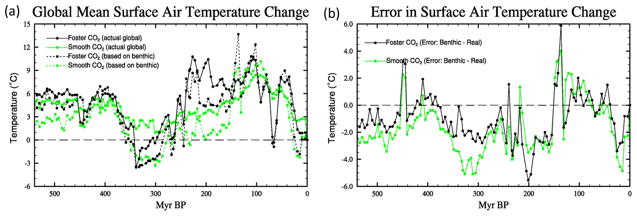
Figure 12Phanerozoic time series of modelled temperature change (relative to pre-industrial) for the smooth (green lines) and Foster CO2 (black) simulations (a) showing the actual modelled global mean surface air temperature (solid lines), whereas the dashed line shows the estimate based on deep ocean temperatures, and (b) error in the estimate of global mean temperature change if based on deep ocean temperatures (i.e. deep ocean – global mean surface temperatures).
The characteristics of the plots can best be understood in terms of Figs. 6 and 10. For instance, most of the Carboniferous simulations plot below the regression line because the polar SSTs are not well correlated with the global mean temperature (Fig. 10). By contrast, the Triassic and Jurassic Foster CO2 simulations plot above the regression line because the deep ocean temperature is not well correlated with the polar temperatures (Fig. 6).
The paper has presented the results from two unique sets of paleoclimate simulations covering the Phanerozoic. The focus of the paper has been to use the HadCM3L climate model to evaluate how well we can predict global mean surface temperatures from benthic foraminifera data. This is an important consideration because benthic microfossil data are one of the few datasets used to directly estimate past global mean temperatures. Other methods, such as using planktonic foraminiferal estimates, are more challenging because the sample sites are geographically sparse, so it is difficult to accurately estimate the global mean temperature from highly variable and widely dispersed data. This is particularly an issue for older time periods when fewer isotopic measurements from planktonic microfossils are available and can result in a bias because most of the isotopic temperature sample localities are from tropical latitudes (30∘ S–30∘ N) (Song et al., 2019).
By contrast, deep ocean temperatures are more spatially uniform. Hence, benthic foraminifera data have frequently been used to estimate past global mean temperatures and climate sensitivity (Hansen et al., 2013). Estimates of uncertainty for deep ocean temperatures incorporate uncertainties from CO2 and from the conversion of δ18O measurements to temperature but have not been able to assess assumptions about the source regions for deep ocean waters and the importance polar amplification. Of course, in practice, lack of an ocean sea floor means that benthic compilations exist only for the last 110 Ma.
Changes in heat transport also play a potentially important role in polar amplification. In the figures in the Supplement, we show the change in atmosphere and ocean poleward heat fluxes for each time period. Examination of the modelled poleward heat transport by the atmosphere and ocean shows a very complicated pattern, with all time periods showing the presence of some Bjerknes compensation (Bjerknes, 1964) (see Outten et al., 2018, for example, in CMIP5 models). Bjerknes compensation is where the change in ocean transport is largely balanced by an equal but opposite change in atmospheric transport. For instance, compared to the present day, the mid-Cretaceous and Early Eocene warm simulations show a large increase in northward atmospheric heat transport, linked with enhanced latent heat transport associated with the warmer, moister atmosphere. However, this is partly cancelled by an equal but opposite change in the ocean transport. For example, compared to present day, the early Eocene Northern Hemisphere atmospheric heat transport increases by up to 0.5 PW (petawatts), but the ocean transport is reduced by an equal amount. The net transport from Equator to the North Pole changes by less than 0.1 PW (i.e. less than 2 % of total). Further back in time, the compensation is still apparent, but the changes are more complicated, especially when the continents are largely in the Southern Hemisphere. Understanding the causes of these transport changes will be the subject of another paper.
We have shown that although the expected correlation between benthic temperatures and high-latitude surface temperatures exists, the correlation has considerable scatter. This is caused by several factors. Changing paleogeographies results in changing locations for deep-water formation. Some paleogeographies result in significant deep-water formation in the Northern Hemisphere (e.g. our present-day configuration), although for most of the Phanerozoic, the dominant source of deep-water formation has been the Southern Hemisphere. Similarly, even when deep water is formed in just one hemisphere, there can be substantial regional and latitudinal variations in its location and the corresponding temperatures. Finally, during times of very warm climates (e.g. mid-Cretaceous), the overturning circulation can be very weak, and there is a marked decoupling between the surface waters and deep ocean. In the HadCM3 model during hothouse time periods, high temperatures and high rates of evaporation produce hot and saline surface waters which sink to become intermediate and deep waters at low latitudes.
Similar arguments can be made regarding the link between global mean temperature and the temperature at high latitudes. Particularly important is the area of land at the poles and the extent of sea ice and/or land ice. Colder climates and paleogeographic configurations with more land at the pole will result in a steeper latitudinal temperature gradient and hence exhibit a changing relationship between polar and global temperatures. But the fraction of land versus ocean is also important.
Finally, the overall relationship between deep ocean temperatures and global mean temperature is shown to be relatively linear, but the slope is quite variable. In the model simulations using the “smooth” CO2 curve, the slope is substantially shallower (0.48) than slope obtained using the Foster CO2 curve (0.76). This is related to the different controls that CO2 and paleogeography exert (as discussed above). In the simulation that uses the smooth CO2 dataset, the levels of CO2 do not vary much, so the paleogeographic controls are more pronounced.
This raises the interesting conundrum that when trying to use reconstructed deep ocean temperatures and CO2 to estimate climate sensitivity, the interpreted global mean temperature also depends, in part, on the CO2 concentrations. However, if we simply use the combined slope, then the root mean square error is approximately 1.4 ∘C, and the maximum error is over 4 ∘C. The root mean square error is a relatively small compared to the overall changes, and hence the resulting uncertainty in climate sensitivity associated with this error is relatively small (∼15 %) and the CO2 uncertainty dominates. However, the maximum error is potentially more significant.
Our work has not addressed other sources of uncertainty. In particular, it would be valuable to use a water isotope-enabled climate model to better address the uncertainties associated with the conversion of the observed benthic δ18O to temperature. This requires assumptions about the δ18O of sea water. We hope to perform such simulations in future work, though this is a particularly challenging computational problem because the isotope-enabled model is significantly slower and the completion of the multi-millennial simulations required for deep ocean estimates would take more than 18 months to complete.
Our simulations extend and develop those published by Lunt et al. (2016) and Farnsworth et al. (2019b, a). The simulations reported in this paper used the same climate model (HadCM3L) but used an improved ozone concentration and corrected a salinity drift that can lead to substantial changes over the duration of the simulation. Our simulations also use an alternative set of geographic reconstructions that cover a larger time period (540 Ma – present day). They also include realistic land ice cover estimates, which were not included in the original simulations (except for the late Cenozoic) but generally have a small impact in the Mesozoic.
Similarly, the new simulations use two alternative models for past atmospheric CO2 use more realistic variations in CO2 through time, compared with idealized constant values in Farnsworth et al. (2019a) and Lunt et al. (2016), while at the same time recognizing the levels of uncertainty. Although the Foster CO2 curve is more directly constrained by CO2 data, it should be noted that these data come from multiple proxies and there are large gaps in the dataset. There is evidence that the different proxies have different biases, and it is not obvious that the correct approach is to simply fit a LOESS-type curve to the CO2 data. This is exemplified by the Maastrichtian. The Foster LOESS curve shows a minimum in CO2 during the Maastrichtian, which results in the modelled deep ocean temperatures being much too cold. However, detailed examination of the CO2 data shows most of the Maastrichtian data are based on stomatal index reconstructions which often are lower than other proxies. Thus, the Maastrichtian low CO2, relative to other periods, is potentially driven by changing the proxy rather than by real temporal changes.
Though the alternative “smooth” CO2 curve is not the optimum fit to the data, it does pass through the cloud of individual CO2 reconstructions and hence represents one possible “reality”. For the Late Cretaceous and Cenozoic, the smooth CO2 simulation set does a significantly better job simulating the deep ocean temperatures of the Friedrich–Cramer–Zachos curve.
Although the focus of the paper has been the evaluation of the modelled relationship between benthic and surface temperatures, the simulations are a potentially valuable resource for future studies. This includes using the simulations for paleoclimate–climate dynamic studies and for climate impact studies, such as ecological niche modelling. We have therefore made the results from our simulations available on our website: https://www.paleo.bristol.ac.uk/ummodel/scripts/papers/Valdes_et_al_2021.html (last access: 30 June 2021).
All simulation data are available from https://www.paleo.bristol.ac.uk/ummodel/scripts/papers/Valdes_et_al_2021.html (last access: 30 June 2021, Valdes et al., 2021).
The supplement related to this article is available online at: https://doi.org/10.5194/cp-17-1483-2021-supplement.
The study was developed by all authors. All model simulations were performed by PJV, who also prepared the manuscript with contributions from all co-authors.
The authors declare that they have no conflict of interest.
Daniel J. Lunt and Paul J. Valdes acknowledge funding from NERC through grant no. NE/P013805/1. The production of paleogeographic digital elevation models was funded by the sponsors of the PALEOMAP project. This work is part of the PhanTASTIC project led by Scott Wing and Brian Huber from the Smithsonian Institution's National Museum of Natural History and was initiated at a workshop supported by Roland and Debra Sauermann. This work was carried out using the computational facilities of the Advanced Computing Research Centre, University of Bristol (http://www.bris.ac.uk/acrc/, last access: 30 June 2021).
This research has been supported by the UK Natural Environment Research Council (NERC) (grant no. NE/P013805/1).
This paper was edited by Yannick Donnadieu and reviewed by two anonymous referees.
Alexeev, V. A., Langen, P. L., and Bates, J. R.: Polar amplification of surface warming on an aquaplanet in “ghost forcing” experiments without sea ice feedbacks, Clim. Dynam., 24, 655–666, https://doi.org/10.1007/s00382-005-0018-3, 2005.
Baatsen, M., van Hinsbergen, D. J. J., von der Heydt, A. S., Dijkstra, H. A., Sluijs, A., Abels, H. A., and Bijl, P. K.: Reconstructing geographical boundary conditions for palaeoclimate modelling during the Cenozoic, Clim. Past, 12, 1635–1644, https://doi.org/10.5194/cp-12-1635-2016, 2016.
Baatsen, M. L. J., von der Heydt, A. S., Kliphuis, M., Viebahn, J., and Dijkstra, H. A.: Multiple states in the late Eocene ocean circulation, Global Planet. Change, 163, 18–28, https://doi.org/10.1016/j.gloplacha.2018.02.009, 2018.
Barron, E. J. and Peterson, W. H.: mid-cretaceous ocean circulation: results from model sensitivity studies, Paleoceanography, 5, 319–337, https://doi.org/10.1029/PA005i003p00319, 1990.
Beerling, D. J., Fox, A., Stevenson, D. S., and Valdes, P. J.: Enhanced chemistry-climate feedbacks in past greenhouse worlds, P. Natl. Acad. Sci. USA, 108, 9770–9775, https://doi.org/10.1073/pnas.1102409108, 2011.
Bjerknes, J.: Atlantic Air-Sea Interaction, Adv. Geophys., 10, 1–82, https://doi.org/10.1016/S0065-2687(08)60005-9, 1964.
Brass, G. W., Southam, J. R., and Peterson, W. H.: Warm Saline Bottom Water in the Ancient Ocean, Nature, 296, 620–623,https://doi.org/10.1038/296620a0, 1982.
Cramer, B. S., Toggweiler, J. R., Wright, J. D., Katz, M. E., and Miller, K. G.: Ocean overturning since the Late Cretaceous: Inferences from a new benthic foraminiferal isotope compilation, Paleoceanography, 24, PA4216, https://doi.org/10.1029/2008PA001683, 2009.
Cramwinckel, M. J., Huber, M., Kocken, I. J., Agnini, C., Bijl, P. K., Bohaty, S. M., Frieling, J., Goldner, A., Hilgen, F. J., Kip, E. L., Peterse, F., van der Ploeg, R., Rohl, U., Schouten, S., and Sluijs, A.: Synchronous tropical and polar temperature evolution in the Eocene, Nature, 559, 382–386, https://doi.org/10.1038/s41586-018-0272-2, 2018.
Dietmuller, S., Ponater, M., and Sausen, R.: Interactive ozone induces a negative feedback in CO2-driven climate change simulations, J. Geophys. Res.-Atmos., 119, 1796–1805, https://doi.org/10.1002/2013jd020575, 2014.
Donnadieu, Y., Puceat, E., Moiroud, M., Guillocheau, F., and Deconinck, J. F.: A better-ventilated ocean triggered by Late Cretaceous changes in continental configuration, Nat. Commun., 7, 10316, https://doi.org/10.1038/ncomms10316, 2016.
Emiliani, C.: Temperatures of Pacific Bottom Waters and Polar Superficial Waters during the Tertiary, Science, 119, 853–855, 1954.
England, M. H.: The Age Of Water And Ventilation Timescales In A Global Ocean Model, J. Phys. Oceanogr., 25, 2756–2777, https://doi.org/10.1175/1520-0485(1995)025<2756:TAOWAV>2.0.CO;2, 1995.
Farnsworth, A., Lunt, D. J., O'Brien, C. L., Foster, G. L., Inglis, G. N., Markwick, P., Pancost, R. D., and Robinson, S. A.: Climate Sensitivity on Geological Timescales Controlled by Nonlinear Feedbacks and Ocean Circulation, Geophys. Res. Lett., 46, 9880–9889, https://doi.org/10.1029/2019gl083574, 2019a.
Farnsworth, A., Lunt, D. J., Robinson, S. A., Valdes, P. J., Roberts, W. H. G., Clift, P. D., Markwick, P., Su, T., Wrobel, N., Bragg, F., Kelland, S. J., and Pancost, R. D.: Past East Asian monsoon evolution controlled by paleogeography, not CO2, Sci Adv, 5, eaax1697, https://doi.org/10.1126/sciadv.aax1697, 2019b.
Foster, G. L., Royer, D. L., and Lunt, D. J.: Future climate forcing potentially without precedent in the last 420 million years, Nat. Commun., 8, 14845, https://doi.org/10.1038/ncomms14845, 2017.
Friedrich, O., Norris, R. D., and Erbacher, J.: Evolution of Cretaceous oceans: A 55 million year record of Earth's temperature and carbon cycle, Grzyb. Found. Spec. Pub., 17, 85–85, 2011.
Friedrich, O., Norris, R. D., and Erbacher, J.: Evolution of middle to Late Cretaceous oceans–A 55 m.y. record of Earth's temperature and carbon cycle, Geology, 40, 107–110, https://doi.org/10.1130/G32701.1, 2012.
Goldner, A., Herold, N., and Huber, M.: The challenge of simulating the warmth of the mid-Miocene climatic optimum in CESM1, Clim. Past, 10, 523–536, https://doi.org/10.5194/cp-10-523-2014, 2014.
Gordon, C., Cooper, C., Senior, C. A., Banks, H., Gregory, J. M., Johns, T. C., Mitchell, J. F. B., and Wood, R. A.: The simulation of SST, sea ice extents and ocean heat transports in a version of the Hadley Centre coupled model without flux adjustments, Clim. Dynam., 16, 147–168, 2000.
Gough, D. O.: Solar Interior Structure and Luminosity Variations, Sol. Phys., 74, 21–34, https://doi.org/10.1007/Bf00151270, 1981.
Gregory, J. M., Ingram, W. J., Palmer, M. A., Jones, G. S., Stott, P. A., Thorpe, R. B., Lowe, J. A., Johns, T. C., and Williams, K. D.: A new method for diagnosing radiative forcing and climate sensitivity, Geophys. Res. Lett., 31, L03205, https://doi.org/10.1029/2003gl018747, 2004.
Hansen, J., Sato, M., Russell, G., and Kharecha, P.: Climate sensitivity, sea level and atmospheric carbon dioxide, Philos. T. Roy. Soc. A, 371, 20120294, https://doi.org/10.1098/rsta.2012.0294, 2013.
Hansen, J., Sato, M., Kharecha, P., Beerling, D., Berner, R., Masson-Delmotte, V., Pagani, M., Raymo, M., Royer, D. L., and Zachos, J. C.: Target atmospheric CO2: Where should humanity aim?, Open Atmos. Sci. J., 2, 217–231, https://doi.org/10.2174/1874282300802010217, 2008.
Hansen, J. E. and Sato, M.: Paleoclimate Implications for Human-Made Climate Change, in: Climate Change, edited by: Berger, A., Mesinger, F., and Sijacki, D., Springer, Vienna, https://doi.org/10.1007/978-3-7091-0973-1_2, 21–47, 2012.
Hardiman, S. C., Andrews, M. B., Andrews, T., Bushell, A. C., Dunstone, N. J., Dyson, H., Jones, G. S., Knight, J. R., Neininger, E., O'Connor, F. M., Ridley, J. K., Ringer, M. A., Scaife, A. A., Senior, C. A., and Wood, R. A.: The Impact of Prescribed Ozone in Climate Projections Run With HadGEM3-GC3.1, J. Adv. Model. Earth Sy., 11, 3443–3453, https://doi.org/10.1029/2019MS001714, 2019.
Harris, J., Ashley, A., Otto, S., Valdes, P., Crossley, R., Preston, R., Watson, J., Goodrich, M., and Team., M. P.: Paleogeography and Paleo-Earth Systems in the Modeling of Marine Paleoproductivity: A Prerequisite for the Prediction of Petroleum Source Rocks, in: Petroleum Systems Analysis – Case Studies, edited by: AbuAli, M. A., Moretti, I., and Nordgård Bolås, H. M., AAPG Memoir, 27–60, https://doi.org/10.1190/ice2015-2210991, 2017.
Henkes, G. A., Passey, B. H., Grossman, E. L., Shenton, B. J., Yancey, T. E., and Perez-Huerta, A.: Temperature evolution and the oxygen isotope composition of Phanerozoic oceans from carbonate clumped isotope thermometry, Earth Planet. Sc. Lett., 490, 40–50, https://doi.org/10.1016/j.epsl.2018.02.001, 2018.
Holland, M. M. and Bitz, C. M.: Polar amplification of climate change in coupled models, Clim. Dynam., 21, 221–232, https://doi.org/10.1007/s00382-003-0332-6, 2003.
Kageyama, M., Albani, S., Braconnot, P., Harrison, S. P., Hopcroft, P. O., Ivanovic, R. F., Lambert, F., Marti, O., Peltier, W. R., Peterschmitt, J.-Y., Roche, D. M., Tarasov, L., Zhang, X., Brady, E. C., Haywood, A. M., LeGrande, A. N., Lunt, D. J., Mahowald, N. M., Mikolajewicz, U., Nisancioglu, K. H., Otto-Bliesner, B. L., Renssen, H., Tomas, R. A., Zhang, Q., Abe-Ouchi, A., Bartlein, P. J., Cao, J., Li, Q., Lohmann, G., Ohgaito, R., Shi, X., Volodin, E., Yoshida, K., Zhang, X., and Zheng, W.: The PMIP4 contribution to CMIP6 – Part 4: Scientific objectives and experimental design of the PMIP4-CMIP6 Last Glacial Maximum experiments and PMIP4 sensitivity experiments, Geosci. Model Dev., 10, 4035–4055, https://doi.org/10.5194/gmd-10-4035-2017, 2017.
Kennett, J. P. and Stott, L. D.: Abrupt Deep-Sea Warming, Palaeoceanographic Changes and Benthic Extinctions at the End of the Paleocene, Nature, 353, 225–229, https://doi.org/10.1038/353225a0, 1991.
Kiehl, J. T. and Shields, C. A.: Sensitivity of the Palaeocene-Eocene Thermal Maximum climate to cloud properties, Philos. T. Roy. Soc. A, 371, 20130093, https://doi.org/10.1098/rsta.2013.0093, 2013.
Knorr, G., Butzin, M., Micheels, A., and Lohmann, G.: A warm Miocene climate at low atmospheric CO2 levels, Geophys. Res. Lett., 38, L20701, https://doi.org/10.1029/2011gl048873, 2011.
Krapp, M. and Jungclaus, J. H.: The Middle Miocene climate as modelled in an atmosphere-ocean-biosphere model, Clim. Past, 7, 1169–1188, https://doi.org/10.5194/cp-7-1169-2011, 2011.
Ladant, J.-B., Poulsen, C. J., Fluteau, F., Tabor, C. R., MacLeod, K. G., Martin, E. E., Haynes, S. J., and Rostami, M. A.: Paleogeographic controls on the evolution of Late Cretaceous ocean circulation, Clim. Past, 16, 973–1006, https://doi.org/10.5194/cp-16-973-2020, 2020.
Lunt, D. J., Valdes, P. J., Dunkley Jones, T., Ridgwell, A., Haywood, A. M., Schmidt, D. N., Marsh, R., and Maslin, M.: CO2-driven ocean circulation changes as an amplifier of Paleocene-Eocene thermal maximum hydrate destabilization, Geology, 38, 875–878, https://doi.org/10.1130/G31184.1, 2010.
Lunt, D. J., Dunkley Jones, T., Heinemann, M., Huber, M., LeGrande, A., Winguth, A., Loptson, C., Marotzke, J., Roberts, C. D., Tindall, J., Valdes, P., and Winguth, C.: A model–data comparison for a multi-model ensemble of early Eocene atmosphere–ocean simulations: EoMIP, Clim. Past, 8, 1717–1736, https://doi.org/10.5194/cp-8-1717-2012, 2012.
Lunt, D. J., Farnsworth, A., Loptson, C., Foster, G. L., Markwick, P., O'Brien, C. L., Pancost, R. D., Robinson, S. A., and Wrobel, N.: Palaeogeographic controls on climate and proxy interpretation, Clim. Past, 12, 1181–1198, https://doi.org/10.5194/cp-12-1181-2016, 2016.
Lunt, D. J., Huber, M., Anagnostou, E., Baatsen, M. L. J., Caballero, R., DeConto, R., Dijkstra, H. A., Donnadieu, Y., Evans, D., Feng, R., Foster, G. L., Gasson, E., von der Heydt, A. S., Hollis, C. J., Inglis, G. N., Jones, S. M., Kiehl, J., Kirtland Turner, S., Korty, R. L., Kozdon, R., Krishnan, S., Ladant, J.-B., Langebroek, P., Lear, C. H., LeGrande, A. N., Littler, K., Markwick, P., Otto-Bliesner, B., Pearson, P., Poulsen, C. J., Salzmann, U., Shields, C., Snell, K., Stärz, M., Super, J., Tabor, C., Tierney, J. E., Tourte, G. J. L., Tripati, A., Upchurch, G. R., Wade, B. S., Wing, S. L., Winguth, A. M. E., Wright, N. M., Zachos, J. C., and Zeebe, R. E.: The DeepMIP contribution to PMIP4: experimental design for model simulations of the EECO, PETM, and pre-PETM (version 1.0), Geosci. Model Dev., 10, 889–901, https://doi.org/10.5194/gmd-10-889-2017, 2017.
Lunt, D. J., Bragg, F., Chan, W.-L., Hutchinson, D. K., Ladant, J.-B., Morozova, P., Niezgodzki, I., Steinig, S., Zhang, Z., Zhu, J., Abe-Ouchi, A., Anagnostou, E., de Boer, A. M., Coxall, H. K., Donnadieu, Y., Foster, G., Inglis, G. N., Knorr, G., Langebroek, P. M., Lear, C. H., Lohmann, G., Poulsen, C. J., Sepulchre, P., Tierney, J. E., Valdes, P. J., Volodin, E. M., Dunkley Jones, T., Hollis, C. J., Huber, M., and Otto-Bliesner, B. L.: DeepMIP: model intercomparison of early Eocene climatic optimum (EECO) large-scale climate features and comparison with proxy data, Clim. Past, 17, 203–227, https://doi.org/10.5194/cp-17-203-2021, 2021.
Murphy, D. P. and Thomas, D. J.: Cretaceous deep-water formation in the Indian sector of the Southern Ocean, Paleoceanography, 27, PA1211, https://doi.org/10.1029/2011pa002198, 2012.
Nowack, P. J., Abraham, N. L., Maycock, A. C., Braesicke, P., Gregory, J. M., Joshi, M. M., Osprey, A., and Pyle, J. A.: A large ozone-circulation feedback and its implications for global warming assessments, Nat. Clim. Change, 5, 41–45, https://doi.org/10.1038/nclimate2451, 2015.
Nunes, F. and Norris, R. D.: Abrupt reversal in ocean overturning during the Palaeocene/Eocene warm period, Nature, 439, 60–63, https://doi.org/10.1038/nature04386, 2006.
O'Brien, C. L., Robinson, S. A., Pancost, R. D., Damste, J. S. S., Schouten, S., Lunt, D. J., Alsenz, H., Bomemann, A., Bottini, C., Brassell, S. C., Farnsworth, A., Forster, A., Huber, B. T., Inglis, G. N., Jenkyns, H. C., Linnert, C., Littler, K., Markwick, P., McAnena, A., Mutterlose, J., Naafs, B. D. A., Puttmann, W., Sluijs, A., van Helmond, N. A. G. M., Vellekoop, J., Wagner, T., and Wrobel, N. E.: Cretaceous sea-surface temperature evolution: Constraints from TEX86 and planktonic foraminiferal oxygen isotopes, Earth-Sci. Rev., 172, 224–247, https://doi.org/10.1016/j.earscirev.2017.07.012, 2017.
Outten, S., Esau, I., and Ottera, O. H.: Bjerknes Compensation in the CMIP5 Climate Models, J. Climate, 31, 8745–8760, https://doi.org/10.1175/jcli-d-18-0058.1, 2018.
Pope, V. D., Gallani, M. L., Rowntree, P. R., and Stratton, R. A.: The impact of new physical parametrizations in the Hadley Centre climate model: HadAM3, Clim. Dynam., 16, 123–146, 2000.
Poulsen, C. J., Barron, E. J., Arthur, M. A., and Peterson, W. H.: Response of the mid-Cretaceous global oceanic circulation to tectonic and CO2 forcings, Paleoceanography, 16, 576–592, https://doi.org/10.1029/2000pa000579, 2001.
Sagoo, N., Valdes, P., Flecker, R., and Gregoire, L. J.: The Early Eocene equable climate problem: can perturbations of climate model parameters identify possible solutions?, Philos. T. Roy. Soc. A, 371, 20130123 https://doi.org/10.1098/rsta.2013.0123, 2013.
Scotese, C. R.: PALEOMAP PaleoAtlas for GPlates and the PaleoData Plotter Program, PALEOMAP Project, EarthByte, available at: https://www.earthbyte.org/paleomap-paleoatlas-for-gplates/ (last access: 30 June 2021), 2016.
Scotese, C. R. and Schettino, A.: Late Permian – Early Jurassic Paleogeography of Western Tethys and the World, in: Permo-Triassic Salt Provinces of Europe, North Africa and the Atlantic Margins, edited by: Soto, J. I., Flinch, J., and Tari, G., Elsevier, 57–95, 2017.
Scotese, C. R. and Wright, N.: PALEOMAP Paleodigital Elevation MOdels (PaleoDEMS) for the Phanerozoic PALEOMAP Project, EarthByte, available at: https://www.earthbyte.org/paleodem-resource-scotese-and-wright-2018 (last access: 30 June 2021), 2018.
Smith, R. S., Gregory, J. M., and Osprey, A.: A description of the FAMOUS (version XDBUA) climate model and control run, Geosci. Model Dev., 1, 53–68, https://doi.org/10.5194/gmd-1-53-2008, 2008.
Song, H. J., Wignall, P. B., Song, H. Y., Dai, X., and Chu, D. L.: Seawater Temperature and Dissolved Oxygen over the Past 500 Million Years, J. Earth Sci., 30, 236–243, https://doi.org/10.1007/s12583-018-1002-2, 2019.
Steinthorsdottir, M., Coxall, H. K., de Boer, A. M., Huber, M., Barbolini, N., Bradshaw, C. D., Burls, N. J., Feakins, S. J., Gasson, E., Henderiks, J., Holbourn, A., Kiel, S., Kohn, M. J., Knorr, G., Kurschner, W. M., Lear, C. H., Liebrand, D., Lunt, D. J., Mors, T., Pearson, P. N., Pound, M. J., Stoll, H., and Stromberg, C. A. E.: The Miocene: the Future of the Past, Paleoceanography and Paleoclimatology, 36, e2020PA004037. https://doi.org/10.1029/2020PA004037, 2021.
Stoll, H. M., Guitian, J., Hernandez-Almeida, I., Mejia, L. M., Phelps, S., Polissar, P., Rosenthal, Y., Zhang, H. R., and Ziveri, P.: Upregulation of phytoplankton carbon concentrating mechanisms during low CO2 glacial periods and implications for the phytoplankton pCO2 proxy, Quat. Sci. Rev., 208, 1–20, https://doi.org/10.1016/j.quascirev.2019.01.012, 2019.
Sutton, R. T., Dong, B. W., and Gregory, J. M.: Land/sea warming ratio in response to climate change: IPCC AR4 model results and comparison with observations, Geophys. Res. Lett., 34, L02701, https://doi.org/10.1029/2006gl028164, 2007.
Upchurch, G. R., Kiehl, J., Shields, C., Scherer, J., and Scotese, C.: Latitudinal temperature gradients and high-latitude temperatures during the latest Cretaceous: Congruence of geologic data and climate models, Geology, 43, 683–686, https://doi.org/10.1130/G36802.1, 2015.
Valdes, P. J., Armstrong, E., Badger, M. P. S., Bradshaw, C. D., Bragg, F., Crucifix, M., Davies-Barnard, T., Day, J. J., Farnsworth, A., Gordon, C., Hopcroft, P. O., Kennedy, A. T., Lord, N. S., Lunt, D. J., Marzocchi, A., Parry, L. M., Pope, V., Roberts, W. H. G., Stone, E. J., Tourte, G. J. L., and Williams, J. H. T.: The BRIDGE HadCM3 family of climate models: HadCM3@Bristol v1.0, Geosci. Model Dev., 10, 3715–3743, https://doi.org/10.5194/gmd-10-3715-2017, 2017.
Valdes, P. J., Scotese, C. R., and Lunt, D. J.: Deep Ocean Temperatures through Time, Bristol Research Initiative for the Dynamic Global Environment (BRIDGE) [data set], available at: https://www.paleo.bristol.ac.uk/ummodel/scripts/papers/Valdes_et_al_2021.html, last access: 30 June 2021.
Verard, C., Hochard, C., Baumgartner, P. O., and Stampfli, G. M.: 3D palaeogeographic reconstructions of the Phanerozoic versus sea-level and Sr-ratio variations, Journal of Palaeogeography, 4, 64–84, https://doi.org/10.3724/Sp.J.1261.2015.00068, 2015.
Westerhold, T., Marwan, N., Drury, A. J., Liebrand, D., Agnini, C., Anagnostou, E., Barnet, J. S. K., Bohaty, S. M., De Vleeschouwer, D., Florindo, F., Frederichs, T., Hodell, D. A., Holbourn, A. E., Kroon, D., Lauretano, V., Littler, K., Lourens, L. J., Lyle, M., Pälike, H., Röhl, U., Tian, J., Wilkens, R. H., Wilson, P. A., and Zachos, J. C.: An astronomically dated record of Earth's climate and its predictability over the last 66 million years, Science, 369, 1383–1387, https://doi.org/10.1126/science.aba6853, 2020.
Witkowski, C. R., Weijers, J. W. H., Blais, B., Schouten, S., and Damste, J. S. S.: Molecular fossils from phytoplankton reveal secular trend over the Phanerozoic, Sci. Adv., 4, eaat4556, https://doi.org/10.1126/sciadv.aat4556, 2018.
You, Y., Huber, M., Muller, R. D., Poulsen, C. J., and Ribbe, J.: Simulation of the Middle Miocene Climate Optimum, Geophys. Res. Lett., 36, L04702, https://doi.org/10.1029/2008gl036571, 2009.
Zachos, J., Pagani, M., Sloan, L., Thomas, E., and Billups, K.: Trends, rhythms, and aberrations in global climate 65 Ma to present, Science, 292, 686–693, 2001.
Zachos, J. C., Dickens, G. R., and Zeebe, R. E.: An early Cenozoic perspective on greenhouse warming and carbon-cycle dynamics, Nature, 451, 279–283, https://doi.org/10.1038/Nature06588, 2008.
Zhou, J., Poulsen, C. J., Pollard, D., and White, T. S.: Simulation of modern and middle Cretaceous marine δ18O with an ocean-atmosphere general circulation model, Paleoceanography, 23, PA3223, https://doi.org/10.1029/2008pa001596, 2008.
Zhu, J., Poulsen, C. J., and Tierney, J. E.: Simulation of Eocene extreme warmth and high climate sensitivity through cloud feedbacks, Sci. Adv., 5, eaax1874, https://doi.org/10.1126/sciadv.aax1874, 2019.
- Article
(10308 KB) - Full-text XML
- EGU Milutin Milankovic Medal 2015
-
Supplement
(154848 KB) - BibTeX
- EndNote