Stripping back the modern to reveal the Cenomanian–Turonian climate and temperature gradient underneath

During past geological times, the Earth experienced several intervals of global warmth, but their driving factors remain equivocal. A careful appraisal of the main processes controlling past warm events is essential to inform future climates and ultimately provide decision makers with a clear understanding of the processes at play in a warmer world. In this context, intervals of greenhouse climates, such as the thermal maximum of the Cenomanian–Turonian (∼94 Ma) during the Cretaceous Period, are of particular interest. Here we use the IPSL-CM5A2 (IPSL: Institut Pierre et Simon Laplace) Earth system model to unravel the forcing parameters of the Cenomanian–Turonian greenhouse climate. We perform six simulations with an incremental change in five major boundary conditions in order to isolate their respective role on climate change between the Cenomanian–Turonian and the preindustrial. Starting with a preindustrial simulation, we implement the following changes in boundary conditions: (1) the absence of polar ice sheets, (2) the increase in atmospheric pCO₂ to 1120 ppm, (3) the change in vegetation and soil parameters, (4) the 1 % decrease in the Cenomanian–Turonian value of the solar constant and (5) the Cenomanian–Turonian palaeogeography. Between the preindustrial simulation and the Cretaceous simulation, the model simulates a global warming of more than 11 ^∘C. Most of this warming is driven by the increase in atmospheric pCO₂ to 1120 ppm. Palaeogeographic changes represent the second major contributor to global warming, whereas the reduction in the solar constant counteracts most of geographically driven warming. We further demonstrate that the implementation of Cenomanian–Turonian boundary conditions flattens meridional temperature gradients compared to the preindustrial simulation. Interestingly, we show that palaeogeography is the major driver of the flattening in the low latitudes to midlatitudes, whereas pCO₂ rise and polar ice sheet retreat dominate the high-latitude response.

1 Introduction

The Cretaceous Period is of particular interest in order to understand drivers of past greenhouse climates because intervals of prolonged global warmth (O'Brien et al., 2017; Huber et al., 2018) and elevated atmospheric CO₂ levels (Wang et al., 2014), possibly similar to future levels, have been documented in the proxy record. The thermal maximum of the Cenomanian–Turonian (CT) interval (94 Ma) represents the acme of Cretaceous warmth, during which one of the most important carbon cycle perturbations of the Phanerozoic occurred, the oceanic anoxic event 2 (OAE2; Jenkyns, 2010; Huber et al., 2018). Valuable understanding of what controls large-scale climate processes can hence be drawn from investigations of the mechanisms responsible for the CT thermal maximum and carbon cycle perturbation.

Proxy-based reconstructions and model simulations of sea-surface temperatures (SSTs) for the CT reveal that during OAE2 the equatorial Atlantic was 4–6^∘ warmer than today (Norris et al., 2002; Bice et al., 2006; Pucéat et al., 2007; Tabor et al., 2016) and possibly even warmer than that (6–9^∘ – Forster et al., 2007). This short and abrupt episode of major climatic, oceanographic and global carbon cycle perturbations occurred at the CT boundary and was superimposed on a long period of global warmth (Jenkyns, 2010). The high latitudes were also much warmer than today (Herman and Spicer, 2010; Spicer and Herman, 2010), as was the abyssal ocean, which experienced bottom temperatures reaching up to 20 ^∘C during the CT (Huber et al., 2002; Littler et al., 2011; Friedrich et al., 2012). Palaeobotanical studies suggest that the atmosphere was also much warmer (Herman and Spicer, 1996), with high-latitude temperatures of up to 17 ^∘C higher than today (Herman and Spicer, 2010) and possibly reaching annual means of 10–12 ^∘C in Antarctica (Huber et al., 1999).

The steepness of the Equator-to-pole gradient is still a matter of debate, in particular because of inconsistencies between data and models as the latter usually predict steeper gradients than those reconstructed from proxy data (Barron, 1993; Huber et al., 1995; Heinemann et al., 2009; Tabor et al., 2016). Models and data generally agree, however, that Cretaceous SST gradients were reduced compared to today (Sellwood et al., 1994; Huber et al., 1995; Jenkyns et al., 2004; O'Brien et al., 2017; Robinson et al., 2019).

The main factor generally considered responsible for the Cretaceous global warm climate is the higher atmospheric CO₂ concentration (Barron et al., 1995; Crowley and Berner, 2001; Royer et al., 2007; Wang et al., 2014; Foster et al., 2017). This has been determined by proxy-data reconstructions of the Cretaceous pCO₂ using various techniques, including analysis of palaeosol δ¹³C (Sandler and Harlavan, 2006; Leier et al., 2009; Hong and Lee, 2012), liverwort δ¹³C (Fletcher et al., 2006) or phytane δ¹³C (Damsté et al., 2008; van Bentum et al., 2012), and leaf stomata analysis (Barclay et al., 2010; Mays et al., 2015; Retallack and Conde, 2020). Modelling studies have also focused on estimating Cretaceous atmospheric CO₂ levels (Barron et al., 1995; Poulsen et al., 2001, 2007; Berner, 2006; Bice et al., 2006; Monteiro et al., 2012) in an attempt to refine the large spread in values inferred from proxy data (from less than 900 to over 5000 ppm). The typical atmospheric pCO₂ concentration resulting from these studies for the CT averages around a long-term value of 1120 ppm (Barron et al., 1995; Bice and Norris, 2003; Royer, 2013; Wang et al., 2014), e.g. 4 times the preindustrial value (280 ppm=1 PAL, “preindustrial atmospheric level”). Atmospheric pCO₂ levels are, however, known to vary on shorter timescales during the period, in particular during OAE2. It has indeed been suggested that this event may have been caused by a large increase in atmospheric pCO₂ concentration, possibly reaching 2000 ppm or even higher, because of volcanic activity in large igneous provinces (Kerr, 1998; Turgeon and Creaser, 2008; Jenkyns, 2010). The proxy records suggest that the pCO₂ levels may have dropped down to 900 ppm after carbon sequestration into organic-rich marine sediments (van Bentum et al., 2012).

Palaeogeography is also considered as a major driver of climate change through geological times (Crowley et al., 1986; Gyllenhaal et al., 1991; Goddéris et al., 2014; Lunt et al., 2016). Several processes linked to palaeogeographic changes have been shown to impact Cretaceous climates. These processes include albedo and evapotranspiration feedbacks from palaeovegetation (Otto-Bliesner and Upchurch, 1997), seasonality due to continental break-up or presence of epicontinental seas (Fluteau et al., 2007), atmospheric feedbacks due to water cycle modification (Donnadieu et al., 2006), Walker and Hadley cells changes after Gondwana breakup (Ohba and Ueda, 2011), or oceanic circulation changes due to gateways opening (Poulsen et al., 2001, 2003). Other potential controlling factors include the time-varying solar constant (Gough, 1981), whose impact on Cretaceous climate evolution was quantified by Lunt et al. (2016), and changes in the distribution of vegetation, which has been suggested to drive warming, especially in the high latitudes with a temperature increase of up to 4–10 ^∘C in polar regions (Otto-Bliesner and Upchurch, 1997; Brady et al., 1998; Upchurch, 1998; Deconto et al., 2000; Hunter et al., 2013).

Despite all these studies, there is no established consensus on the relative importance of each of the controlling factors for the CT climate. In particular, the primary driver of the Cretaceous climate has been suggested to be either pCO₂ or palaeogeography. Early studies suggested a negligible role of palaeogeography on global climate compared to the high CO₂ concentration (Barron et al., 1995), whereas others suggested that CO₂ was not the primary control (Veizer et al., 2000) or that the impact of palaeogeography on climate was as important as a doubling of pCO₂ (Crowley et al., 1986). More recent modelling studies have also suggested that palaeogeographic changes could affect global climate (Poulsen et al., 2003; Donnadieu et al., 2006; Fluteau et al., 2007), but their impact remains debated (Ladant and Donnadieu, 2016; Lunt et al., 2016; Tabor et al., 2016). For example, the simulations of Lunt et al. (2016) support a key role of palaeogeography at the regional rather than global scale and show that the global palaeogeographic signal is cancelled by an opposite trend due to changes in the solar constant. Tabor et al. (2016) also suggested important regional climatic impacts of palaeogeography, but argued that CO₂ is the main driver of the Late Cretaceous climate evolution. In contrast, Ladant and Donnadieu (2016) find a large impact of palaeogeography on the global mean Late Cretaceous temperatures; their signal is roughly comparable to a doubling of atmospheric pCO₂. Finally, the role of palaeovegetation is also uncertain as some studies show a major role at high latitudes (Upchurch, 1998; Hunter et al., 2013), whereas a more recent study instead suggests limited impact at high latitudes (<2 ^∘C) with a cooling effect at low latitudes under high pCO₂ values (Zhou et al., 2012).

In this study, we investigate the forcing parameters of CT greenhouse climate by using a set of simulations run with the IPSL-CM5A2 Earth system model. We perform six simulations, using both preindustrial and CT boundary conditions, where we incrementally modify the preindustrial boundary conditions to that of the CT. The changes are as follows: (1) the removal of polar ice sheets, (2) an increase in pCO₂ to 1120 ppm, (3) the change in vegetation and soil parameters, (4) a 1 % reduction in the value of the solar constant, and (5) the implementation of Cenomanian–Turonian palaeogeography. We particularly focus on processes driving warming or cooling of atmospheric surface temperatures after each change in boundary condition change to study the relative importance of each parameter in the CT to preindustrial climate change. We also investigate how the SST gradient responds to boundary condition changes to understand the evolution of its steepness between the CT and the preindustrial.

2 Model description and experimental design

2.1 IPSL-CM5A2 Model

IPSL-CM5A2 is an updated version of the IPSL-CM5A-LR Earth system model developed at IPSL (Institut Pierre-Simon Laplace) within the CMIP5 framework (Dufresne et al., 2013). It is a fully coupled Earth system model, which simulates the interactions between atmosphere, ocean, sea ice and land surface. The model includes the marine carbon and other key biogeochemical cycles (C, P, N, O, Fe and Si – see Aumont et al., 2015). Its former version, IPSL-CM5A-LR, has a rich history of applications, including present-day and future climates (Aumont and Bopp, 2006; Swingedouw et al., 2017) as well as preindustrial (Gastineau et al., 2013) and palaeoclimate studies (Kageyama et al., 2013; Contoux et al., 2015; Bopp et al., 2017; Tan et al., 2017; Sarr et al., 2019). It was also part of IPCC AR5 and CMIP5 projects (Dufresne et al., 2013). IPSL-CM5A-LR has been used to explore not only links between marine productivity and climate (Bopp et al., 2013; Le Mézo et al., 2017; Ladant et al., 2018), vegetation and climate (Contoux et al., 2013; Woillez et al., 2014), and topography and climate (Maffre et al., 2018) but also the role of nutrients in the global carbon cycle (Tagliabue et al., 2010) and the variability of oceanic circulation and upwelling (Ortega et al., 2015; Swingedouw et al., 2015). Building on recent technical developments, IPSL-CM5A2 provides enhanced computing performances compared to IPSL-CM5A-LR, allowing 1000-year-long integrations required for deep-time palaeoclimate applications or long-term future projections (Sepulchre et al., 2019). It thus reasonably simulates modern-day and historical climates (despite some biases in the tropics), whose complete description and evaluation can be found in Sepulchre et al. (2019).

IPSL-CM5A2 is composed of the LMDZ atmospheric model (Hourdin et al., 2013), the ORCHIDEE land surface and vegetation model (including the continental hydrological cycle, vegetation and carbon cycle; Krinner et al., 2005), and the NEMO ocean model (Madec and the NEMO team, 2008), including the LIM2 sea-ice model (Fichefet and Maqueda, 1997) and the PISCES marine biogeochemistry model (Aumont et al., 2015). The OASIS coupler (Valcke et al., 2006) ensures a good synchronization of the different components, and the XIOS input/output parallel library is used to read and write data. The LMDZ atmospheric component has a horizontal resolution of 96×95, (equivalent to 3.75^∘ in longitude and 1.875^∘ in latitude) and 39 uneven vertical levels. ORCHIDEE shares the same horizontal resolution, whereas NEMO – the ocean component – has 31 uneven vertical levels (from 10 m at the surface to 500 m at the bottom) and a horizontal resolution of approximately 2^∘, enhanced to up to 0.5^∘ in latitude in the tropics. NEMO uses the ORCA2.3 tripolar grid to overcome the North Pole singularity (Madec and Imbard, 1996).

2.2 Experimental design

Six simulations were performed for this study: one preindustrial control simulation, named piControl, and five simulations for which the boundary conditions were changed one at a time to progressively reconstruct the CT climate (see Table 1 for details). The scenarios are called 1X-NOICE (with no polar ice sheets), 4X-NOICE (no polar ice sheets + pCO₂ at 1120 ppm), 4X-NOICE-PFT-SOIL (previous changes + implementation of idealized plant functional types (PFTs) and mean parameters for soil), 4X-NOICE-PFT-SOIL-SOLAR (previous changes + reduction in the solar constant) and 4X-CRETACEOUS (previous changes + CT palaeogeography). The piControl simulation has been run for 1800 years and the five others for 2000 years in order to reach near-surface equilibrium (see Fig. 1).

Table 1 Description of the simulations. The parameters in bold indicate the specific change for the corresponding simulation. Simulations are run for 2000 years, except piControl, which is run for 1000 years.

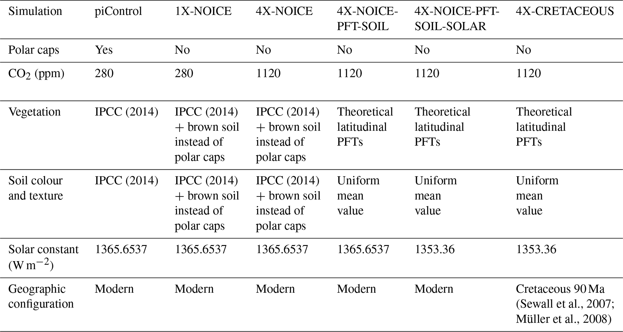
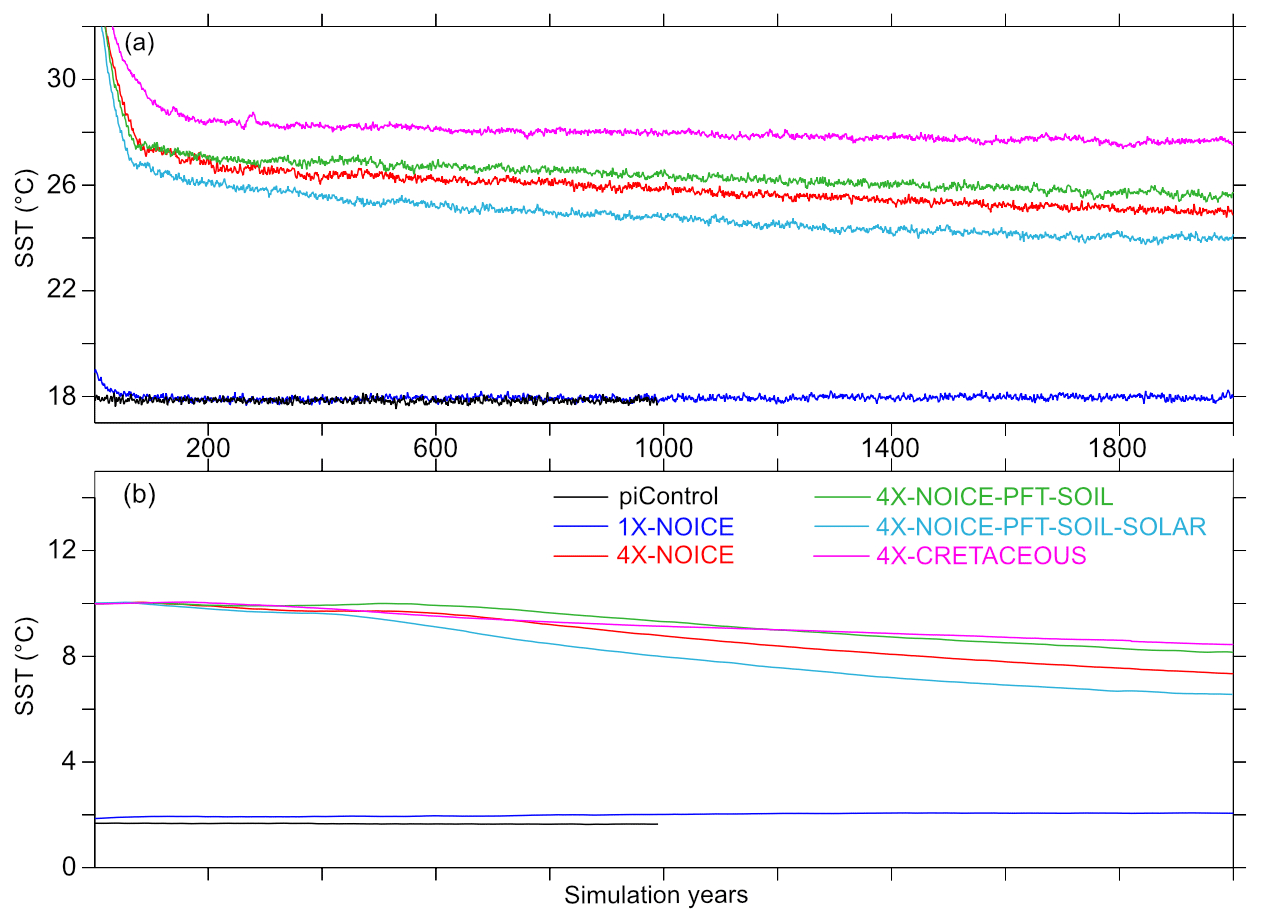
Figure 1 Time series for mean annual oceanic temperatures. (a) Sea-surface temperature and (b) deep-ocean (2500 m) temperature. The piControl and 1X-NOICE simulations are perfectly equilibrated. The 4X simulations still have a small linear drift, around 0.1 ^∘C per century or less: 0.07, 0.08, 0.05 and 0.01 ^∘C per century during the last 500 years for SST of 4XNOICE, 4X-NOICE-PFT-SOIL, 4X-NOICE-PFT-SOIL-SOLAR and 4X-CRETACEOUS respectively; 0.11, 0.08, 0.07 and 0.06 ^∘C per century during the last 500 years, for deep ocean of 4X-NOICE, 4X-NOICE-PFT-SOIL, 4X-NOICE-PFT-SOILSOLAR and 4X-CRETACEOUS respectively.

2.2.1 Boundary conditions

As most evidence suggests the absence of permanent polar ice sheets during the CT (MacLeod et al., 2013; Ladant and Donnadieu, 2016; Huber et al., 2018), we remove polar ice sheets in our simulations (except in piControl), and we adjust topography to account for isostatic rebound resulting from the loss of the land ice covering Greenland and Antarctica (see Fig. S1 in the Supplement). Ice sheets are replaced with brown bare soil, and the river routing stays unchanged.

In the 4X simulations (i.e. all except piControl and 1X-NOICE), pCO₂ is fixed to 1120 ppm (4 PAL), a value reasonably close to the mean suggested by a recent compilation of CT pCO₂ reconstructions (Wang et al., 2014).

In the 4X-NOICE-PFT-SOIL simulation, the distribution of the 13 standard PFTs defined in ORCHIDEE is uniformly reassigned along latitudinal bands, based on a rough comparison with the preindustrial distribution of vegetation, in order to obtain a theoretical latitudinal distribution usable for any geological period. The list of PFTs and associated latitudinal distribution and fractions are described in Table S1 in the Supplement. Mean soil parameters, i.e. mean soil colour and texture (rugosity), are calculated from preindustrial maps (Zobler, 1999; Wilson and Henderson-Sellers, 2003) and uniformly prescribed on all continents. The impact of these idealized PFTs and mean parameters is discussed in the results.

The 4X-NOICE-PFT-SOIL-SOLAR simulation is initialized from the same conditions as 4X-NOICE-PFT-SOIL except that the solar constant is reduced to its CT value (Gough, 1981). We use here the value of 1353.36 W m⁻² (98.9 % of the modern solar luminosity, calculated for an age of 90 Myr).

The 4X-CRETACEOUS simulation, finally, incorporates the previous modifications plus the implementation of the CT palaeogeography. The land–sea configuration used here is that proposed by Sewall et al. (2007), in which we have implemented the bathymetry from Müller et al. (2008) (see Fig. 2). These bathymetric changes are done to represent deep-oceanic topographic features, such as ridges, that are absent from the Sewall palaeogeographic configuration. In this simulation, the mean soil colour and rugosity as well as the theoretical latitudinal PFTs distribution are adapted to the new land–sea mask, and the river routing is recalculated from the new topography. We also modify the tidally driven mixing associated with dissipation of internal wave energy for the M2 and K1 tidal components from present-day values (de Lavergne et al., 2019). The parameterization used for simulations with the modern geography follows Simmons et al. (2004), with refinements in the modern Indonesian Throughflow (ITF) region according to Koch-Larrouy et al. (2007). To create a Cenomanian–Turonian tidal dissipation forcing, we calculate an M2 tidal dissipation field using the Oregon State University Tidal Inversion System (OTIS, Egbert et al., 2004; Green and Huber, 2013). The M2 field is computed using our Cenomanian–Turonian bathymetry and an ocean stratification taken from an unpublished equilibrated Cenomanian–Turonian simulation realized with the IPSLCM5A2 with no M2 field. In the absence of any estimation for the CT, we prescribe the K1 tidal dissipation field to be 0. In addition, the parameterization of Koch-Larrouy et al. (2007) is not used here because the ITF does not exist in the Cretaceous.

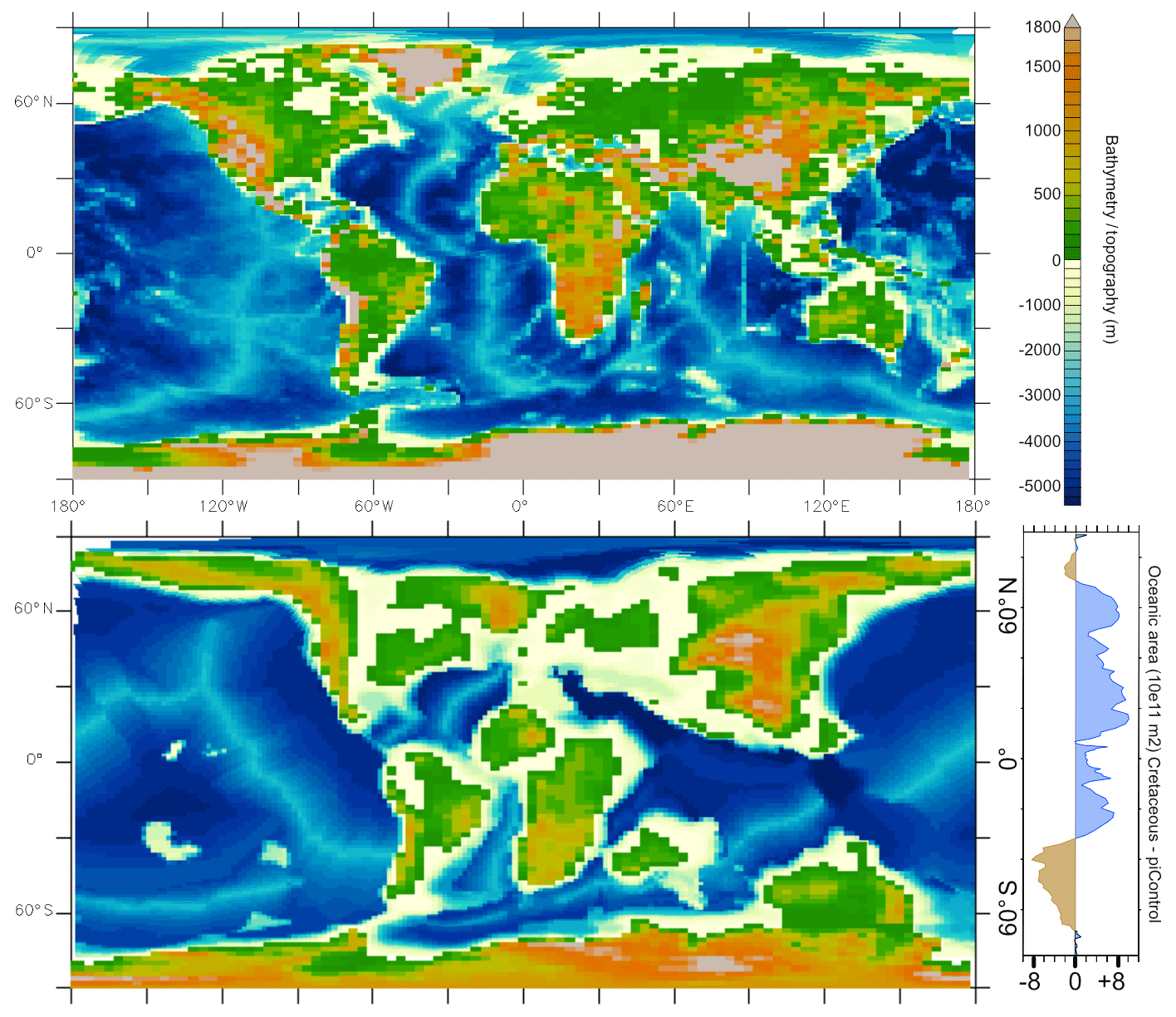
Figure 2 Modern and Cenomanian–Turonian geographic configurations used for the piControl and 4X-CRETACEOUS simulations respectively and meridional oceanic area anomaly between Cretaceous palaeogeography and modern geography.

2.2.2 Initial conditions

The piControl and 1X-NOICE simulations are initialized with conditions from the Atmospheric Model Intercomparison Project (AMIP), which were constrained by realistic sea-surface temperature (SST) and sea ice from 1979 to near present (Gates et al., 1999). In an attempt to reduce the integration time required to reach near-equilibrium, the initial conditions of simulations with 4 PAL are taken from warm idealized conditions (higher SST and no sea ice) adapted from those described in Lunt et al. (2017). The constant initial salinity field is set to 34.7 PSU, and ocean temperatures are initialized with a depth-dependent distribution (see Sepulchre et al., 2019). In waters deeper than 1000 m, the temperature, T=10 ^∘C, whereas at depths shallower than 1000 m it follows

$$\begin{array}{}\text{(1)}& T=\mathrm{10}+\left({\displaystyle \frac{\mathrm{1000}-\text{depth}}{\mathrm{1000}}}\right)\cdot \mathrm{25}\cos \left(\text{latitude}\right).\end{array}$$

3 Results

The simulated changes between the preindustrial (piControl) and the CT (4X-CRETACEOUS) simulations can be decomposed into five components based on our boundary condition changes: (1) polar ice sheet removal (Δice), (2) pCO₂ (ΔCO₂), (3) PFT and soil parameters (ΔPFT-SOIL), (4) solar constant (Δsolar) and (5) palaeogeography (Δpaleo). Each contribution to the total climate change can be calculated by a linear factorization (Broccoli and Manabe, 1987; Von Deimling et al., 2006), which simply corresponds to the anomaly between two consecutive simulations. The choice of applying a linear factorization approach was made due to computing time and cost. We appreciate that another sequence of changes could lead to different intermediate states and could modulate the intensity of warming or cooling associated with each change. The computational costs would be too high for this study to explore this further here; it is an interesting problem that we leave for a future investigation. The results presented in the following are averages calculated over the last 100 simulated years.

3.1 Global changes

The progressive change in parameters made to reconstruct the CT climate induces a general global warming (Table 2, Fig. 3). The annual global atmospheric temperature at 2 m above the surface (T2M) rises from 13.25 to 24.35 ^∘C between the preindustrial and CT simulations. All changes in boundary conditions generate a warming signal on a global scale, with the exception of the decrease in solar constant, which generates a cooling. Most of the warming is due to the 4-fold increase in atmospheric pCO2, which alone increases the global mean temperature by 9 ^∘C. Palaeogeographic changes also represent a major contributor to the warming, leading to an increase in T2M of 2.6 ^∘C. In contrast, the decrease in solar constant leads to a cooling of 1.8 ^∘C at the global scale. Finally, changes in the soil parameters and PFTs, as well as the retreat of polar caps, have smaller impacts, leading to increases in global mean T2M of 0.8 and 0.5 ^∘C respectively.

Table 2 Simulations results (global annual mean over last 100 years of simulation).

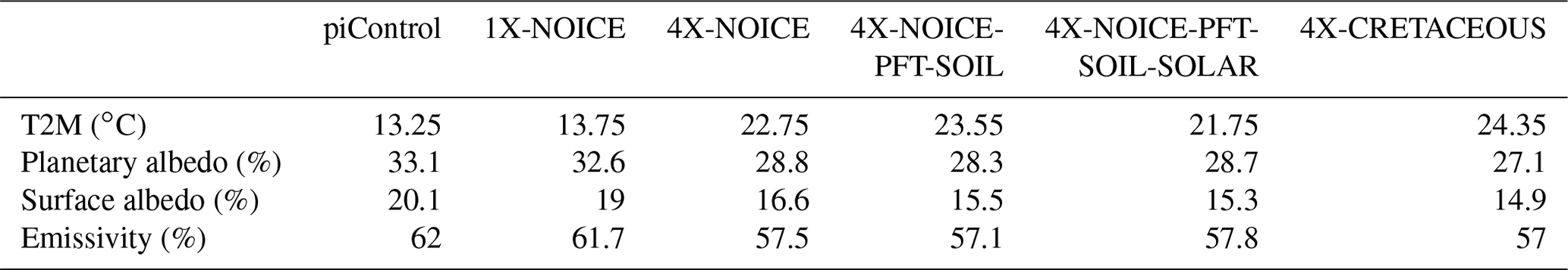
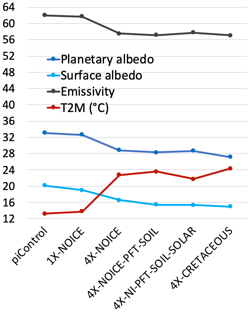
Figure 3 Evolution of albedo (surface and planetary) and emissivity, in percentages and of T2M (^∘C) from piControl to 4X-CRETACEOUS simulations. The major change is always recorded with the change in pCO₂ between 1X-NOICE and 4X-NOICE simulations.

Temperature changes exhibit different geographic patterns (Fig. 4) depending on which parameter is changed. These patterns range from global and uniform cooling (Δsolar – Fig. 4e) to a global, polar-amplified warming (ΔpCO₂ – Fig. 4c), as well as heterogeneous regional responses (Δice or Δpaleo – Fig. 4b and f). In the next section, we describe the main patterns of change and the main feedbacks arising.

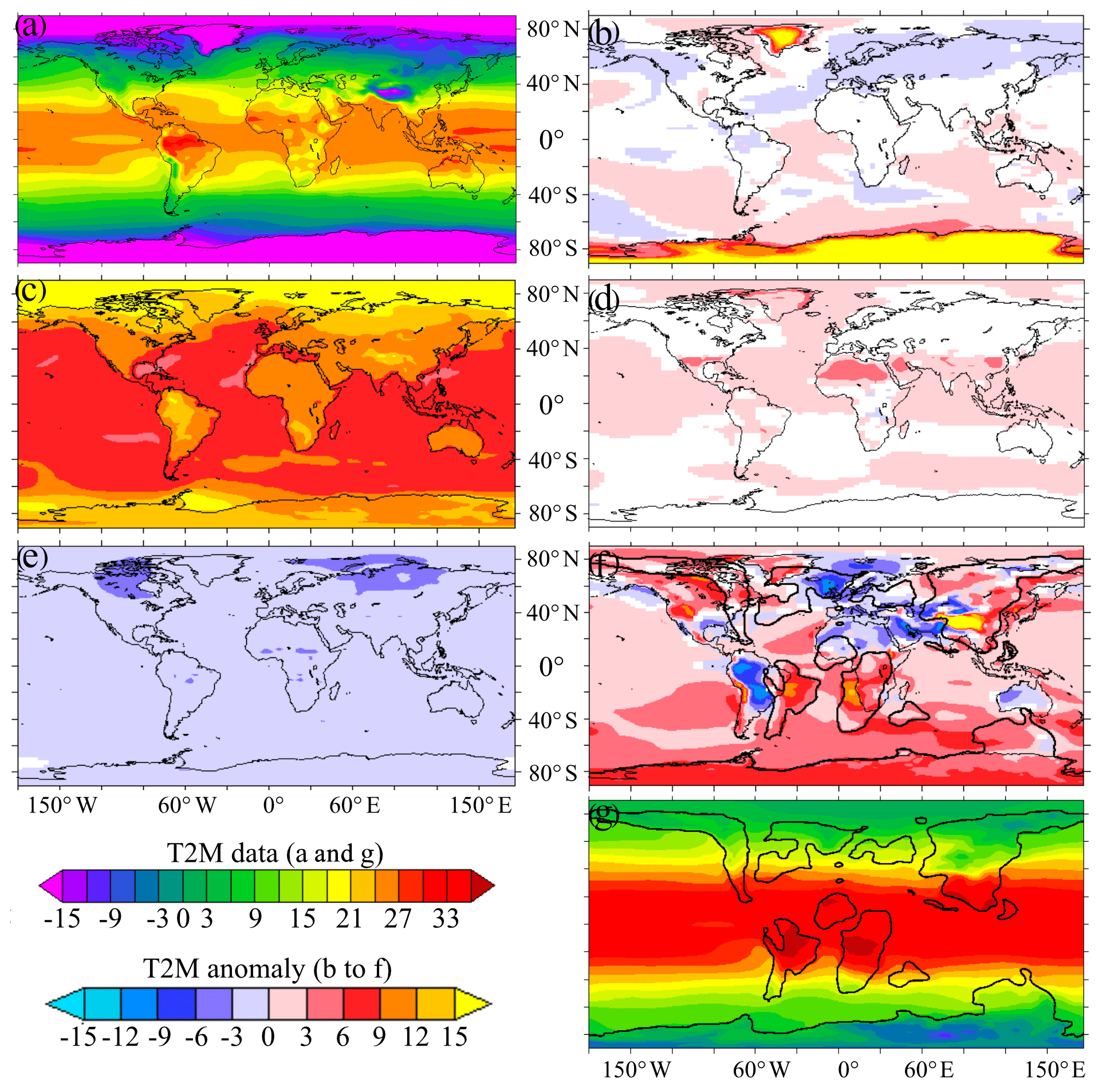
Figure 4 T2M (^∘C) for (a) piControl initial simulation and (g) Cretaceous final simulation and anomalies (^∘C) for intermediate simulations: (b) 1X-NOICE − piControl, (c) 4X-NOICE − 1X-NOICE, (d) 4X-NOICE-PFT-SOIL − 4X-NOICE, (e) 4X-NOICE-PFT-SOIL-SOLAR − 4X-NOICE-PFT-SOIL and (f) 4X-CRETACEOUS − 4X-NOICE-PFT-SOIL. White colour (not represented in the colour bar) correspond to areas where the anomaly is not statistically significative according to Student's t test.

3.2 The major contributor to global warming – ΔCO₂

As mentioned above, the 4-fold increase in pCO₂ leads to a global warming of 9 ^∘C (Table 2, Fig. 3) between the 1X-NOICE and the 4X-NOICE simulations. The whole Earth warms, with an amplification located over the Arctic and Austral oceans and a warming generally larger over continents than over oceans (Fig. 4c). The warming is due to a general decrease in planetary albedo and of the atmosphere's emissivity (see Fig. S2). The decrease in the emissivity of the atmosphere is directly driven by the increase in CO₂ and thus greenhouse trapping in the atmosphere. It is also amplified by an increase in high-altitude cloudiness (defined as cloudiness at atmospheric pressure <440 hPa) over the Antarctic continent (Fig. 5a, b). The decrease in planetary albedo is due to two major processes. First, a decrease in sea ice and snow cover (especially over Northern Hemisphere continents and along the coasts of Antarctica), leading to surface albedo decrease, explains the warming amplification over polar oceans and continents. Second, a decrease in low-altitude cloudiness (defined as cloudiness at atmospheric pressure >680 hPa) at all latitudes except over the Arctic (Fig. 5a, b) leads to an increase in absorbed solar radiation.

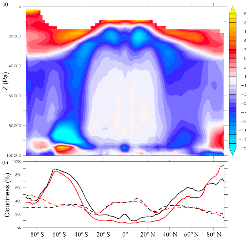
Figure 5 Mean annual cloudiness for 1X-NOICE and 4X-NOICE simulations. (a) Anomaly of total cloudiness (4X-NOICE − 1X NOICE). (b) Low-altitude cloudiness (below 680 hPa of atmospheric pressure – solid curves) and high-altitude cloudiness above 440 hPa of atmospheric pressure – dashed curves) for 1X-NOICE (black) and 4X-NOICE (red) simulations.

The contrast in the atmospheric response over continents and oceans is due to the impact of the evapotranspiration feedback. Oceanic warming drives an increase in evaporation, which acts as a negative feedback and moderates the warming by consuming more latent heat at the ocean surface. In contrast, high temperatures resulting from continental warming tend to inhibit vegetation development, which acts as positive feedback and enhances the warming due to reduced transpiration and reduced latent heat consumption.

3.3 Boundary conditions with the smallest global impact – Δice, ΔPFT-SOIL and Δsolar

The removal of polar ice sheets in the 1X-NOICE simulation leads to a weak global warming of 0.5 ^∘C but a strong regional warming observed over areas previously covered by the Antarctic and Greenland ice sheets (Fig. 4a, b). This signal is due to the combination of a decrease in elevation (i.e. lapse rate feedback – Fig. S3) and in surface albedo, which is directly linked to the shift from a reflective ice surface to a darker bare soil surface. Unexpected cooling is also simulated in specific areas, such as the margins of the Arctic Ocean and the southwestern Pacific. These contrasted climatic responses to the impact of ice sheets on sea-surface temperatures are consistent with previous modelling studies (Goldner et al., 2014; Knorr and Lohmann, 2014; Kennedy et al., 2015). Their origin is still unclear, but changes in winds in the Southern Ocean, due to topographic changes after polar ice sheet removal, may locally impact oceanic currents, deep-water formation, and thus oceanic heat transport and temperature distribution. In the Northern Hemisphere, the observed cooling over Eurasia could be linked to stationary wave feedbacks following changes in topography after Greenland ice sheet removal (Fig. S4; see also Maffre et al., 2018).

The change in soil parameters and the implementation of theoretical zonal PFTs in the 4X-NOICE-PFT-SOIL simulation drive a warming of 0.8 ^∘C. This warming is essentially located above arid areas, such as the Sahara, Australia or the Middle East, and polar latitudes (Antarctica/Greenland) (Fig. 4d) and is mostly caused by the implementation of a mean uniform soil colour, which drives a surface albedo decrease over deserts that normally have a lighter colour. The warming at high latitudes is linked to vegetation change: bare soil that characterizes continental regions previously covered with ice is replaced by boreal vegetation with a lower surface albedo. The presence of vegetation at such high latitudes is consistent with high-latitude palaeobotanical data and temperature records during the Cretaceous (Otto-Bliesner and Upchurch, 1997; Herman and Spicer, 2010; Spicer and Herman, 2010).

Finally, the change in solar constant from 1365 to 1353 W m⁻² (Gough, 1981) directly drives a cooling of 1.8 ^∘C evenly distributed over the planet (Fig. 4e).

3.4 The most complex response – Δpalaeogeography

The palaeogeographic change drives a global warming of 2.6 ^∘C. This is seen year-round in the Southern Hemisphere, while the Northern Hemisphere experiences a warming during winter and cooling during summer compared to the 4X-NI-PFT-SOIL-SOLAR simulation (Fig. 6). These temperature changes are linked to a general decrease in planetary albedo and/or emissivity, although the Northern Hemisphere sometimes exhibits increased albedo, due to the increase in low-altitude cloudiness. This increase in albedo is compensated by a strong atmosphere emissivity decrease during winter but not during summer, which leads to the seasonal pattern of cooling and warming (Fig. S5).

Figure 6 T2M (^∘C) mean annual meridional gradients for 4X-NI-PFT-SOIL-SOLAR (black) and 4X-CRETACEOUS (red) simulations. Solid curve corresponds to annual average; dashed curves correspond to winter and summer values. The 4X-CRETACEOUS simulation is generally warmer than the 4X-NI-PFT-SOIL-SOLAR-SOLAR simulation, with the exception of the boreal summer.

The albedo and emissivity changes are linked to atmospheric and oceanic circulation modifications driven by four major features of the CT palaeogeography (Fig. 2):

• 1.

  Equatorial oceanic gateway opening (Central American Seaway/Neotethys)

• 2.

  Polar gateway closure (Drake/Tasman)

• 3.

  Increase in oceanic area in the Northern Hemisphere (Fig. 2)

• 4.

  Decrease in oceanic area in the Southern Hemisphere (Fig. 2)

In the CT simulation, we observe an intensification of the meridional surface circulation and extension towards higher latitudes compared to the simulation with the modern geography (Fig. 8a, b), as well as an intensification of subtropical gyres, especially in the Pacific (Fig. S6), which are responsible for an increase in poleward oceanic heat transport (OHT – Fig 8c). Such modifications can be linked to the opening of equatorial gateways that creates a zonal connection between the Pacific, Atlantic and Neotethys oceans (Enderton and Marshall, 2008; Hotinski and Toggweiler, 2003) and that leads to the formation of a strong circumglobal equatorial current (Fig. 7b). This connection permits the existence of stronger easterly winds that enhance equatorial upwelling and drive increased export of water and heat from low latitudes to polar regions. In the Southern Hemisphere, the Drake Passage is only open to shallow flow, and the Tasman Gateway has not yet formed. The closure of these zonal connections leads to the disappearance of the modern Antarctic Circumpolar Current (ACC) during the Cretaceous (Fig. 7c, d). Notwithstanding, the observed increase in southward OHT between 40 and 60^∘S (Fig. 8c) is explained by the absence of significant zonal connections in the Southern Ocean, which allows for the buildup of polar gyres in the CT simulation (Fig. S6).

The increase in OHT is associated with a meridional expansion of high sea-surface temperatures leading to an intensification of evaporation between the tropics and a poleward shift of the ascending branches of the Hadley cells. The combination of these two processes results in a greater injection of moisture into the atmosphere between the tropics (Fig. S7). Consequently, the high-altitude cloudiness increases and spreads towards the tropics, leading to an enhanced greenhouse effect. This process is the main driver of the intertropical warming (Herweijer et al., 2005; Levine and Schneider, 2010; Rose and Ferreira, 2013).

The response of the atmosphere to the palaeogeographic changes in the midlatitudes and high latitudes is different in the Southern and Northern hemispheres because the ocean-to-land ratio varies between the CT configuration and the modern one. In the Southern Hemisphere, the reduced ocean surface area in the CT simulation (Fig. 2) limits evaporation and moisture injection into the atmosphere, which in turn leads to a decrease in relative humidity and low-altitude cloudiness (Fig. S8) and associated year-round warming due to reduced planetary albedo. In the Northern Hemisphere, oceanic surface area increases (Fig. 2) and results in a strong increase in evaporation and moisture injection into the atmosphere. Low-altitude cloudiness and planetary albedo increase and lead to summer cooling, as discussed above (Fig. 6). During winter an increase in high-altitude cloudiness leads to an enhanced greenhouse effect and counteracts the larger albedo. This high-altitude cloudiness increase is consistent with the simulated increase in extratropical OHT (Fig. 8). Midlatitude convection and moist air injection into the upper troposphere are consequently enhanced and efficiently transported poleward (Rose and Ferreira, 2013; Ladant and Donnadieu, 2016). In addition, increased continental fragmentation in the CT palaeogeography relative to the preindustrial decreases the effect of continentality (Donnadieu et al., 2006) because thermal inertia is greater in the ocean than over continents.

3.5 Temperature gradients

3.5.1 Ocean

The mean annual global SST increases as much as 9.8 ^∘C (from 17.9 to 27.7  ^∘C) across the simulations. The SST warming is slightly weaker than that of the mean annual global atmospheric temperature at 2 m discussed above and most likely occurs because of evaporation processes due to the weaker atmospheric warming simulated above oceans compared to that simulated above continents. Unsurprisingly, as for the atmospheric temperatures, pCO₂ is the major controlling parameter of the ocean warming (7 ^∘C), followed by palaeogeography (4.5 ^∘C) and changes in the solar constant (2.3 ^∘C), although the last of which induces a cooling rather than a warming. PFT and soil parameter changes and the removal of polar ice sheets have a minor impact on the global SST (0.6 and 0 ^∘C respectively). It is interesting to note the increased contribution of palaeogeography to the simulated SST warming compared to its contribution to the simulated atmospheric warming, which is probably driven by the major changes simulated in surface ocean circulation (Fig. 7).

Figure 7 Surface currents for (a, c) 4X-NOICE-PFT-SOIL-SOLAR and (b, d) 4X-CRETACEOUS simulations. (a, b) Intensity of surface circulation in sverdrups (Sv – annual mean for 0–80 m of water depth). Strong equatorial winds lead to the formation of an equatorial circumglobal current. (c, d) Intensity of surface circulation (Sv – annual mean for 0–80 m of water depth). The closure of the Drake Passage (DP-300 m of water depth) leads to the suppression of the ACC.

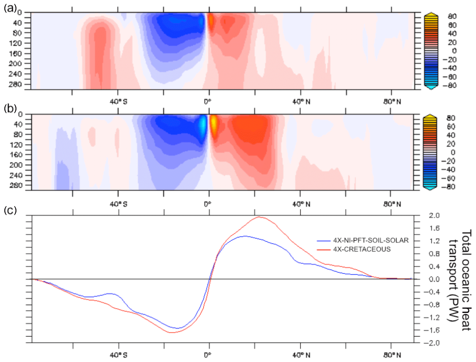
Figure 8 (a, b) Global mean annual meridional stream-function (Sv) for the first 300 m of water depth. Red and blue colours indicate clockwise and anticlockwise circulation respectively. (a) 4X-NI-PFT-SOIL-SOLAR and (b) 4X-CRETACEOUS. (c) Oceanic heat transport for 4X-NI-PFT-SOIL-SOLAR and 4X-CRETACEOUS simulations. Positive and negative values indicate northward and southward transport direction respectively.

Mean annual SSTs in the preindustrial simulation reach ∼26 ^∘C in the tropics (calculated as the zonal average between 30^∘ S and 30^∘ N) and $\sim -\mathrm{1.5}$ ^∘C at the poles (beyond 70^∘ N – Fig. 9a). In this work, we define the meridional temperature gradients as the linear temperature change per 1^∘ of latitude between 30 and 80^∘. The gradients in the piControl experiment then amount to 0.45 and 0.44 ^∘C per ^∘ latitude for the Northern and Southern hemispheres respectively. In the CT simulation, the mean annual SSTs reach ∼33.3 ^∘C in the tropics and ∼5 and 10 ^∘C in the Arctic and Southern Ocean respectively, and the simulated CT meridional gradients are 0.45 and 0.39 ^∘C per ^∘ latitude for the Northern and Southern hemispheres respectively.

Figure 9 (a) Mean annual meridional sea-surface temperature gradients for all simulations. (b) Same SST curves as (a) but superimposed such that Equator temperatures are equal, allowing to compare the steepness of the curves. (c) Meridional atmospheric surface temperature gradients for all simulations. (d) Same curves as (c) but superimposed such that Equator temperatures are equal.

The progressive flattening of the SST gradient can be visualized by superimposing the zonal mean temperatures of the different simulations and by adjusting them at the Equator (Fig. 9b). Two major observations can be drawn from these results. First, palaeogeography has a strong impact on the low-latitude (<30^∘ of latitude) SST gradient because it widens the latitudinal band of relatively homogeneous warm tropical SST as a result of the opening of equatorial gateways. Second, poleward of 40^∘ in latitude, the palaeogeography and the increase in atmospheric pCO₂ both contribute to the flattening of the SST gradient with a larger influence from palaeogeography than from atmospheric pCO₂.

3.5.2 Atmosphere

In the preindustrial simulation, mean tropical atmospheric temperatures reach ∼23.6 ^∘C, whereas polar temperatures (calculated as the average between 80 and 90^∘ of latitude) in the Northern and Southern hemispheres reach around −16.8 and −37 ^∘C respectively. The northern meridional temperature gradient is 0.69 ^∘C per ^∘ latitude, while the southern latitudinal temperature gradient is 1.07 ^∘C per ^∘ latitude (Fig. 9c). This significant difference is explained by the very negative mean annual temperatures over Antarctica linked to the presence of the ice sheet.

In the CT simulation, mean tropical atmospheric temperatures reach ∼32.3 ^∘C, whereas polar temperatures reach ∼3.4 ^∘C in the Northern Hemisphere and $\sim -\mathrm{0.5}$ ^∘C in the Southern Hemisphere, thereby yielding latitudinal temperature gradients of 0.49 and 0.54 ^∘C per ^∘ latitude respectively. The gradients are reduced compared to the preindustrial because the absence of year-round sea and land ice at the poles drives leads to far higher polar temperatures.

As for the SST gradients, we plot atmospheric meridional gradients by adjusting temperature values so that temperatures at the Equator are equal for each simulation (Fig. 9d). This normalization reveals that the mechanisms responsible for the flattening of the gradients are different for each hemisphere. In the Southern Hemisphere high latitudes (>60^∘ of latitude), three parameters contribute to reducing the Equator-to-pole temperature gradient in the following order of importance: removal of polar ice sheets, palaeogeography and increase in atmospheric pCO₂. In contrast, the reduction in the gradient steepness in the Northern Hemisphere high latitudes is exclusively explained by the increase in atmospheric pCO₂. In the low and midlatitudes, this temperature gradient reduction is essentially explained by palaeogeography in the Southern Hemisphere and by a similar contribution of palaeogeographic changes and increase in atmospheric pCO₂ in the Northern Hemisphere.

4 Discussion

4.1 Cenomanian–Turonian model–data comparison

The results predicted by our CT simulation can be compared to reconstructions of atmospheric and oceanic palaeotemperatures inferred from proxy data (Fig. 10a, b). Our SST data compilation is modified version of Tabor et al. (2016), with additional data from more recent studies (see our data in the Supplement). We also compiled atmospheric temperature data obtained from palaeobotanical and palaeosoil studies (see our data in the Supplement for the complete database and references).

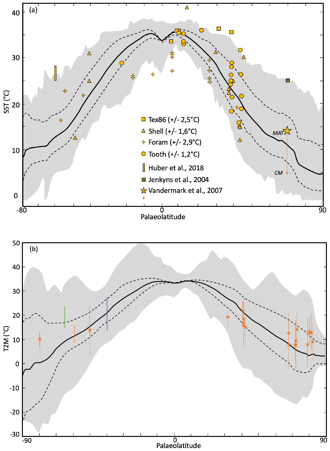
Figure 10 Meridional surface temperature gradients for the 4X-CRETACEOUS simulation. (a) Oceanic temperatures: the solid line corresponds to the mean annual temperature obtained from the modelling. Dashed lines correspond to winter and summer seasonal averages. The grey shaded areas correspond to local monthly temperatures. Data points are obtained with several proxies for the Cenomanian–Turonian Period. The green data point is obtained from TEX86 for the Maastrichtian (70 Ma) and extrapolated for 90 Ma. The Huber et al. (2018) point is obtained from δ¹⁸O on foraminifera and the Vandermark et al. (2007) point is interpreted from the presence of crocodilian fossils. MAT: mean annual temperature; CM: coldest month. (b) Atmospheric temperatures: same legend as (a) for modelised temperatures. Data points are obtained from several proxies including CLAMP analysis on palaeofloras, leaf analyses, palaeosol-derived climofunction or bioclimatic analysis. Symbols represent mean annual temperatures and solid lines associated ranges/errors. Dashed lines represent monthly mean temperatures. Orange data points are for Cenomano–Turonian ages (100–90 Ma), blue data points for Albian and green data points for Coniacian–Santonian (88–85 Ma).

The Cretaceous equatorial and tropical SST have long been believed to be similar or even lower than those of today (Sellwood et al., 1994; Crowley and Zachos, 1999; Huber et al., 2002), thus feeding the problem of “tropical overheating” systematically observed in general circulation model simulations (Barron et al., 1995; Bush et al., 1997; Poulsen et al., 1998). This incongruence was based on the relatively low tropical temperatures reconstructed from foraminiferal calcite (25–30 ^∘C, Fig. 9a), but subsequent work suggested that these were underestimated because of diagenetic alteration (Pearson et al., 2001; Pucéat et al., 2007). Latest data compilations including temperature reconstructions from other proxies, such as TEX86, have provided support for high tropical SST in the Cenomanian–Turonian (Tabor et al., 2016; O'Brien et al., 2017), and our tropical SST are mostly consistent with existing palaeotemperature reconstructions (Fig. 10a). In the midlatitudes (30–60^∘), proxy records infer a wide range of possible SSTs, ranging from 10 ^∘C to more than 30 ^∘C. Simulated temperatures in our CT simulation reasonably agree with these reconstructions if seasonal variability, represented by local monthly maximum and minimum temperatures (grey shaded areas, Fig. 10a), is considered. This congruence would imply that a seasonal bias may exist in temperatures reconstructed from proxies, which is suggested in previous studies (Sluijs et al., 2006; Hollis et al., 2012; Huber, 2012; Steinig et al., 2020) but still debated (Tierney, 2012). There are unfortunately only a few high-latitude SST data points available, which render the model–data comparison difficult. In the Northern Hemisphere, the presence of crocodilian fossils (Vandermark et al., 2007) in the northern Labrador Sea (∼70^∘ of latitude) imply mean annual temperature of at least 14 ^∘C and temperature of the coldest month of at least 5 ^∘C. In comparison, simulated temperatures at the same latitude in the adjacent Western Interior Sea are very similar (13.5 ^∘C for the annual mean and 7.9 ^∘C for the coldest month). In the Southern Hemisphere, mean annual SSTs calculated from foraminiferal calcite at DSDP sites 511 and 258 are between 25 and 28 ^∘C (Huber et al., 2018). Simulated annual SST reach a monthly maximum of 28 ^∘C around the location of site DSDP 258. We speculate that a seasonal bias in the foraminiferal record may represent a possible cause for this difference; alternatively, local deviations of the regional seawater δ¹⁸O from the globally assumed −1 ‰ value may also reduce the model–data discrepancy (Zhou et al., 2008; Zhu et al., 2020).

To our knowledge, atmospheric temperature reconstructions from tropical latitudes are not available. In the midlatitudes (30–60^∘), simulated atmospheric temperatures in the Southern Hemisphere reveal reasonable agreement with data, whereas Northern Hemisphere mean zonal temperatures in our model are slightly warmer than that inferred from proxies (Fig. 10b). At high latitudes, the same trend is observed for atmospheric temperatures as it is for SST with data indicating higher temperatures than the model in both the Southern and Northern hemispheres. This interhemispheric symmetry in model–data discrepancy could indicate a systematic cool bias of the simulated temperatures.

4.2 Reconstructed latitudinal temperature gradients

The simulated Northern Hemisphere latitudinal SST gradient of (∼0.45 ^∘C per ^∘ latitude) is in good agreement with those reconstructed from palaeoceanographic data in the Northern Hemisphere (∼0.42 ^∘C per ^∘ latitude), whereas it is much larger in the Southern Hemisphere (∼0.39 ^∘C per ^∘ latitude vs. ∼0.3 ^∘C per ^∘ latitude) (Fig. 11). This overestimate of the latitudinal gradient holds for the atmosphere as well, as gradients inferred from data are much lower (North=0.2 ^∘C per ^∘ latitude and South=0.18 ^∘C per ^∘ latitude) than simulated gradients (North=0.49 ^∘C per ^∘ latitude and South=0.55 ^∘C per ^∘ latitude), although the paucity of Cenomanian–Turonian continental temperatures proxy data is likely to significantly bias this comparison.

Figure 11 Plot of atmospheric and sea-surface mean annual temperature gradients vs. pCO₂ for different modelling studies and data compilation. Data gradients are plotted for a default pCO₂ value of 4 PAL. Gradients are expressed in degrees Celsius per degree latitude (^∘C per ^∘ latitude) and are calculated from 30 to 80^∘ of latitude. Gradients linked by a line correspond to studies realized with the same model & palaeogeography. Solid lines or gradients marked with a (E) correspond to an Eocene palaeogeography. Dashed lines or gradients marked with a C correspond to a Cretaceous palaeogeography.

In the following, we compare our simulated gradients to those obtained in previous deep-time modelling studies using recent Earth system models. Because Earth system models studies focusing on the Cenomanian–Turonian are limited in numbers, we include simulations of the Early Eocene (∼55 Ma), which is another interval of global climatic warmth (Lunt et al., 2012a, 2017) (Fig. 11). The simulated SST latitudinal gradients range from 0.32 to 0.55 ^∘C per ^∘ latitude (Lunt et al., 2012a; Tabor et al., 2016; Zhu et al., 2019; Fig. 11) and the atmospheric latitudinal gradients from 0.33 to 0.78 ^∘C per ^∘ latitude (Huber and Caballero, 2011; Lunt et al., 2012a; Niezgodzki et al., 2017; Upchurch et al., 2015; Zhu et al., 2019; Fig. 11). For a single model and a single set of boundary conditions (Cretaceous or Eocene), the lowest latitudinal gradient is obtained for the highest pCO₂ value. However, when comparing different studies with the same model (Cretaceous vs. Eocene using the ECHAM5 model; Lunt et al., 2012a; Niezgodzki et al., 2017) it is not the case: the Southern Hemisphere atmospheric gradient obtained for the Eocene with the ECHAM5 model is always lower than those obtained for the Cretaceous with the same model, regardless of the pCO₂ value (Fig. 11 and the Supplement). These results show the major role of boundary conditions (in particular palaeogeography) in defining the latitudinal temperature gradient. IPSL-CM5A2 predicts SST and atmosphere gradients that are well within the range of other models of comparable resolution and complexity. Models almost systematically simulate larger gradients than those obtained from data (Fig. 11, see also Huber, 2012). The reasons behind this incongruence are debated (Huber, 2012) but highlight the need for more data and for challenging the behaviour of complex Earth system models, in particular in the high latitudes. Studies have demonstrated that models are able to simulate lower latitudinal temperature gradients under specific conditions such as anomalously high CO₂ concentrations (Huber and Caballero, 2011), modified cloud properties and radiative parameterizations (Upchurch et al., 2015; Zhu et al., 2019), or lower palaeo elevations and/or more extensive wetlands (Hay et al., 2019). Finally, from a proxy perspective, it has been suggested that a sampling bias could exist, with a better record of temperatures during the warm season at high latitudes and during the cold season in low latitudes (Huber, 2012). Such possible biases would help reduce the model–data discrepancy, in particular for atmospheric temperatures (Fig. 10b), as high-latitude reconstructed temperatures are more consistent with simulated summer temperatures, whereas the consistency is better with simulated winter temperatures in the low latitudes to midlatitudes, but further work is required to unambiguously demonstrate the existence of these biases.

4.3 Primary climate controls

The earliest estimates of climate sensitivity (or the temperature change under a doubling of the atmospheric pCO₂) predicted a 1.5 to 4.5 ^∘C temperature increase, with the most likely scenario providing an increase of 2.5 ^∘C (Charney et al., 1979; Barron et al., 1995; Sellers et al., 1996; IPCC, 2014). Our modelling study predicts an atmospheric warming of 11.1 ^∘C for the CT. The signal is notable due to a 9 ^∘C warming in response to the 4-fold increase in pCO₂, which converts to an increase of 4.5 ^∘C for a doubling of pCO₂ (assuming a linear response). This climate sensitivity agrees with the higher end of the range of previous estimates (Charney et al., 1979; Barron et al., 1995; Sellers et al., 1996; IPCC, 2014). However, our simulated climate sensitivity could be slightly lower as the simulations are not completely equilibrated (Fig. 1). The latest generation of Earth system models used in deep-time palaeoclimate also show an increasingly higher climate sensitivity to increased CO₂ (Hutchinson et al., 2018; Golaz et al., 2019; Zhu et al., 2019), suggesting that the sensitivity could have been underestimated in earlier studies. For example, the recent study of Zhu et al. (2019), using an up-to-date parameterization of cloud microphysics in the CESM1.2 model, proposes an Eocene climate sensitivity of 6.6 ^∘C for a doubling of CO₂ from 3 to 6 PAL.

We have shown that pCO₂ is the main controlling factor for atmospheric global warming, whereas the effects of the palaeogeography (warming) and reduced solar constant (cooling) nearly cancel each other out at the global scale (see also Lunt et al., 2016). These results agree with previous studies suggesting that pCO₂ is the main factor controlling climate (Barron et al., 1995; Crowley and Berner, 2001; Royer et al., 2007; Foster et al., 2017). However, we also demonstrate that palaeogeography plays a major role in the latitudinal distribution of temperatures and impacts oceanic temperatures (with a similar magnitude as a doubling of pCO₂), thus confirming that it is also a critical driver of the Earth's climate (Poulsen et al., 2003; Donnadieu et al., 2006; Fluteau et al., 2007; Lunt et al., 2016). The large climatic influence of the continental configuration has not been reported for palaeogeographic configurations closer to each other, e.g. the Maastrichtian and Cenomanian (Tabor et al., 2016). The main features influencing climate in our study (i.e. the configuration of equatorial and polar zonal connections and the land/sea distribution) are indeed not fundamentally different in the two geological periods investigated by Tabor et al. (2016). Palaeogeography is thus a first-order control on climate over long timescales.

Early work has suggested that high-latitude warming can be amplified in deep-time simulations by rising CO₂ via cloud and vegetation feedbacks (Otto-Bliesner and Upchurch, 1997; Deconto et al., 2000) or by increasing ocean heat transport (Barron et al., 1995; Schmidt and Mysak, 1996; Brady et al., 1998), in particular when changing the palaeogeography (Hotinski and Toggweiler, 2003). Our study confirms that the palaeogeography is a primary control on the steepness of the oceanic meridional temperature gradient. Furthermore, palaeogeography is the only process, among those investigated, that controls both the atmosphere and ocean temperature gradients in the tropics, and it has a greater impact than atmospheric CO₂ on the reduction of the atmospheric temperature gradient at high latitudes in the Southern Hemisphere between the CT and the preindustrial. The increase in pCO₂ appears as the second most important parameter controlling the SST gradient at high latitudes and is the main control of the reduced atmospheric gradient in the Northern Hemisphere due to low cloud albedo feedback. The effect of palaeovegetation on the reduced temperature gradient is marginal at high latitudes in our simulations, in contrast to the significant warming reported in early studies (Otto-Bliesner and Upchurch, 1997; Upchurch, 1998; Deconto et al., 2000) but in agreement with more recent model simulations suggesting a limited influence of vegetation in the Cretaceous high-latitude warmth (Zhou et al., 2012). However, our modelling setup prescribes boreal vegetation at latitudes higher than 50^∘, whereas evidence exists to support the development of evergreen forests poleward of 60^∘ of latitude (Sewall et al., 2007; Hay et al., 2019) and of temperate forests at up to 60^∘ of latitude (Otto-Bliesner and Upchurch, 1997). The presence of such vegetation types could change not only the albedo of continental regions but also heat and water vapour transfer by altered evapotranspiration processes, thus leading to warming amplification at high latitudes and reduced temperature gradients (Otto-Bliesner and Upchurch, 1997; Hay et al., 2019). Based on these studies and on our results, we cannot exclude that different types of high latitude could promote a greater impact of palaeovegetation in reducing the temperature gradient.

5 Conclusions

To quantify the impact of major climate forcings on the Cenomanian–Turonian climate, we perform a series of six simulations using the IPSL-CM5A2 Earth system model in which we incrementally implement changes in boundary conditions on a preindustrial simulation to obtain ultimately a simulation of the Cenomanian–Turonian stage of the Cretaceous. This study confirms the primary control exerted by atmospheric pCO₂ on atmospheric and sea-surface temperatures, followed by palaeogeography. In contrast, the flattening of meridional SST gradients between the preindustrial and the CT is mainly due to palaeogeographic changes and to a lesser extent to the increase in pCO₂. The atmospheric gradient response is more complex because the flattening is controlled by several factors including palaeogeography, pCO₂ and polar ice sheet retreat. While predicted oceanic and atmospheric temperatures show reasonable agreement with data in the low and midlatitudes, predicted temperatures in the high latitudes are colder than palaeotemperatures reconstructed from proxies, which leads to steeper Equator-to-pole gradients in the model than those inferred from proxies. However, this mismatch, often observed in data–model comparison studies, has been reduced in the last few decades and could be further resolved by considering possible sampling/seasonal biases in the proxies and by continuously improving model physics and parameterizations.