NALPS19: sub-orbital-scale climate variability recorded in northern Alpine speleothems during the last glacial period

Sub-orbital-scale climate variability of the last glacial period provides important insights into the rates at which the climate can change state, the mechanisms that drive such changes, and the leads, lags, and synchronicity occurring across different climate zones. Such short-term climate variability has previously been investigated using δ¹⁸O from speleothems (δ¹⁸O_calc) that grew along the northern rim of the Alps (NALPS), enabling direct chronological comparisons with δ¹⁸O records from Greenland ice cores (δ¹⁸O_ice). In this study, we present NALPS19, which includes a revision of the last glacial NALPS δ¹⁸O_calc chronology over the interval 118.3 to 63.7 ka using 11, newly available, clean, precisely dated stalagmites from five caves. Using only the most reliable and precisely dated records, this period is now 90 % complete and is comprised of 16 stalagmites from seven caves. Where speleothems grew synchronously, the timing of major transitional events in δ¹⁸O_calc between stadials and interstadials (and vice versa) are all in agreement on multi-decadal timescales. Ramp-fitting analysis further reveals that, except for one abrupt change, the timing of δ¹⁸O transitions occurred synchronously within centennial-scale dating uncertainties between the NALPS19 δ¹⁸O_calc record and the Asian monsoon composite speleothem δ¹⁸O_calc record. Due to the millennial-scale uncertainties in the ice core chronologies, a comprehensive comparison with the NALPS19 chronology is difficult. Generally, however, we find that the absolute timing of transitions in the Greenland Ice Core Chronology (GICC) 05_modelext and Antarctic Ice Core Chronology (AICC) 2012 are in agreement on centennial scales. The exception to this is during the interval of 100 to 115 ka, where transitions in the AICC2012 chronology occurred up to 3000 years later than in NALPS19. In such instances, the transitions in the revised AICC2012 chronology of Extier et al. (2018) are in agreement with NALPS19 on centennial scales, supporting the hypothesis that AICC2012 appears to be considerably too young between 100 and 115 ka. Using a ramp-fitting function to objectively identify the onset and the end of abrupt transitions, we show that δ¹⁸O shifts took place on multi-decadal to multi-centennial timescales in the North Atlantic-sourced regions (northern Alps and Greenland) as well as the Asian monsoon. Given the near-complete record of δ¹⁸O_calc variability during the last glacial period in the northern Alps, we also offer preliminary considerations regarding the controls on mean δ¹⁸O_calc for given stadials and interstadials. We find that, as expected, δ¹⁸O_calc values became increasingly lighter with distance from the oceanic source regions, and increasingly lighter with increasing altitude. Exceptions were found for some high-elevation sites that locally display δ¹⁸O_calc values that are heavier than expected in comparison to lower-elevation sites, possibly caused by a summer bias in the recorded signal of the high-elevation site, or a winter bias in the low-elevation site. Finally, we propose a new mechanism for the centennial-scale stadial-level depletions in δ¹⁸O such as the Greenland Stadial (GS)-16.2, GS-17.2, GS-21.2, and GS-23.2 “precursor” events, as well as the “within-interstadial” GS-24.2 cooling event. Our new high-precision chronology shows that each of these δ¹⁸O depletions occurred in the decades and centuries following rapid rises in sea level associated with increased ice-rafted debris and southward shifts of the Intertropical Convergence Zone, suggesting that influxes of meltwater from moderately sized ice sheets may have been responsible for the cold reversals causing the Atlantic Meridional Overturning Circulation to slow down similar to the Preboreal Oscillation and Older Dryas deglacial events.

1 Introduction

Speleothems from the northern rim and central European Alps have provided a number of important, high-resolution, precisely ²³⁰Th-dated records of both orbital- and millennial-scale climate variability during the last glacial and interglacial periods (Spötl and Mangini, 2002; Spötl et al., 2006; Boch et al., 2011; Moseley et al., 2014; Luetscher et al., 2015; Moseley et al., 2015; Häuselmann et al., 2015). The oxygen isotopic signature of such records (herein referred to as δ¹⁸O_calc) has helped improve the fundamental understanding of the effect that changes in atmospheric (Luetscher et al., 2015) and North Atlantic circulation (Moseley et al., 2015) have on European climate, whilst the robust chronologies have provided important information about the timescales upon which the climate can change in this well-populated region (Boch et al., 2011; Moseley et al., 2014). Furthermore, the pattern and timing of excursions in δ¹⁸O_calc of northern Alpine speleothems during the last glacial cycle have been shown to be synchronous within dating uncertainties (Boch et al., 2011; Moseley et al., 2014) with the sawtooth pattern of changes in the δ¹⁸O of Greenland ice cores (herein referred to as δ¹⁸O_ice; known as Dansgaard–Oeschger cycles; Johnsen et al., 1992; Dansgaard et al., 1993), thus reflecting the shared North Atlantic moisture source and integrated climate system (Boch et al., 2011). The sawtooth pattern of δ¹⁸O is generally interpreted in both Greenland and the northern Alps as being caused by a rapid increase in temperature and humidity leading into a mild climate state (interstadial), followed by a gradual cooling leading into a cold and dry glacial state (stadial). In total, 25 such cycles of rapid warming and gradual cooling, as well as many other smaller centennial- and decadal-scale events, are recognised as having occurred during the last glacial period (Dansgaard et al., 1993; NGRIP Project members, 2004; Capron et al., 2010a). This has resulted in a new stratigraphic framework (INTIMATE event stratigraphy) for abrupt climate changes in Greenland, in which shorter-scale events that occur within the 25 main stadials and interstadials are designated “a to e” (Rasmussen et al., 2014). This nomenclature will be used in the remainder of this article.

When considering the timing of the transitions in δ¹⁸O between stadial and interstadial states, the largest offsets between the northern Alps speleothem chronology (NALPS) and Greenland Ice Core Chronology (layer-counted GICC05, 0 to 60 ka; Svensson et al., 2008 and modelled GICC05_modelext, 60 to 122 ka; Wolff et al., 2010) are 767 years in Marine Isotope Stage (MIS) 3 (Moseley et al., 2014) and 1060 years in MIS 5 (Boch et al., 2011). The former is associated with the warming transition into Greenland Interstadial 16.1c (GI-16.1c), and the latter with the cooling transition into Greenland Stadial 22 (GS-22; Rasmussen et al., 2014). The timing for both of these transitions in the NALPS chronology was constrained from speleothems high in detrital thorium (Boch et al., 2011; Moseley et al., 2014). Since one of the prerequisites for reliable ²³⁰Th dating is that minimal ²³⁰Th is incorporated into the calcite at the time of deposition (Ivanovich and Harmon, 1992; Dorale et al., 2004), it is reasonable to question the accuracy of the age of these two transitions. In the case of the MIS 3 sample (Moseley et al., 2014), the correction for the initial incorporation of daughter nuclides was well constrained by isochron methods (Ludwig and Titterington, 1994; Dorale et al., 2004), however, in the case of the MIS 5 sample (Boch et al., 2011), the detrital Th was corrected for using an a priori assumption that the contaminant phase had the same composition of silicate bulk earth (Wedepohl, 1995). Furthermore, the accuracy of the GICC05_modelext chronology is questionable in the vicinity of GI-22 to 21 (Capron et al., 2010b; Vallelonga et al., 2012). Specifically, the duration of GS-22 appears to be underestimated, probably as a result of an overestimation of the annual layer thickness by the ss09sea06bm ice flow model (Johnsen et al., 2001) upon which GICC05_modelext is based in the portion of the record older than 60 ka (Wolff et al., 2010; Vallelonga et al., 2012). Vallelonga et al. (2012) thus revised the duration of GS-22 from 2620 years to 2894±99 years using annual layer-counting of seasonal cycles in the chemical impurities in the ice. Given the uncertainties in the chronologies for both the NALPS speleothems and NGRIP ice core during GI-22 to GI-21, it is thus difficult to determine the reliability and extent of the leads, lags, and synchronicity at this time. In addition to the complexities around GS-22, the chronology of events between GI-25 and 23 are also poorly constrained. This is visible when comparing the GICC05_modelext chronology (Wolff et al., 2010) with the Antarctic Ice Core Chronology (AICC) 2012 chronology (Veres et al., 2013), which differ by up to 2700 years, and also when comparing the pattern of the δ¹⁸O shifts during GS-24 in NALPS and NGRIP (Boch et al., 2011).

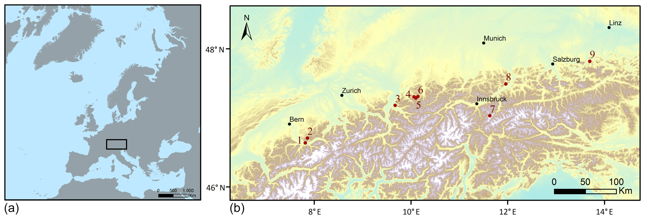
Figure 1 Map of cave sites discussed in text. 1. St. Beatus cave; 2. Siebenhengste cave; 3. Große Baschg cave; 4. Schneckenloch cave; 5. Klaus Cramer cave; 6. Hölloch cave; 7. Kleegruben cave (part of wider discussion on isotopic controls); 8. Grete–Ruth shaft; 9. Gassel cave. The generalised map (a) is produced with EuroGeographics and UN-FAO GI data; city locations (b) are taken from the Urban Audit, 2004 – European Commission, Eurostat/GISCO data set; the digital elevation model (b) is produced using Copernicus data and information funded by the European Union – EU DEM layers.

Here, we revisit the NALPS speleothem chronology over the interval 63.7 to 118.3 thousand years ago BP (ka; Boch et al., 2011) using new samples that are low in detrital thorium and/or have a more pronounced δ¹⁸O_calc signal, with the aim of improving the chronology such that better informed conclusions about leads/lags and synchronicity in the climate system may be made. The original record was discontinuous, with coverage of 76 % of the 54.6 kyr interval. Gaps in the record were present between 111.6 and 110.0, 94.5 and 89.7, 84.7 and 83.0, 77.5 and 76.0, and 75.5 and 72.0 ka (Boch et al., 2011). With the addition of new speleothems, we extend the coverage to 90 %, improve the accuracy and precision of some climate transitions, and designate the revised chronology “NALPS19”.

2 Regional climate

The European Alps, situated between 44 and 48^∘ N, are a 950 km long mountain range running ENE–WSW located close to the southern fringe of the European mainland. The highest peaks, reaching over 4000 m in elevation, are situated in the western Alps of France and Switzerland, whilst the eastern Alps, located in Austria, are on average 1000 m lower. Across the whole of the Alps, the average elevation is ca. 2500 m above sea level (a.s.l.); thus this mountain range forms a major topographic barrier between the North Atlantic and Mediterranean climate zones (Wanner et al., 1997). Today, the Alps are located to the south of the extra-tropical westerlies, which bring precipitation sourced from the North Atlantic to the northern and western flanks, particularly during winter and spring (Wanner et al., 1997; Sodemann and Zubler, 2010). Lagrangian back-trajectory studies have shown that for the period 1995–2002, the North Atlantic contributed ca. 40 % of the annual mean moisture to the Alps, whilst the Mediterranean contributed 23 %, the Arctic, Nordic and Baltic seas 16 %, and the European land masses 21 % (Sodemann and Zubler, 2010). Contributions to the northern and southern sides of the Alps, however, displayed considerable seasonal differences. Throughout the year, the North Atlantic contributes more moisture to the northern Alps as compared to the southern Alps, and this is especially pronounced in winter and spring (Sodemann and Zubler, 2010). During summer, central European land masses are the dominant moisture source across the entire Alps, though the North Atlantic still makes some contribution to the northern flanks, and the Mediterranean to the southern flanks. In autumn, the northern Alps receive comparable quantities of moisture from both the North Atlantic and Mediterranean, whilst the southern Alps are dominated by moisture from the Mediterranean (Sodemann and Zubler, 2010). On longer, multi-decadal timescales, moisture sources and trajectories to the Alps have been shown to be highly variable. In particular, the phase of the North Atlantic Oscillation (NAO), which is especially pronounced in winter (Wanner et al., 1997), exhibits one of the strongest controls. During the positive phase, when positive sea-surface temperature and air-pressure anomalies build up in the south-western North Atlantic, and negative ones in the north, the associated temperature gradient across the western North Atlantic is high. This leads to an intensification of the North Atlantic polar front jet stream, which creates a high pressure zone over the Alps and Mediterranean causing higher temperatures and less precipitation (Wanner et al., 1997). Conversely, during a negative NAO phase the air pressure decreases over the Alps and Mediterranean leading to lower air temperatures and higher precipitation.

Table 1 Details of caves and speleothem samples analysed in this study, presented from west to east. See Boch et al. (2011) for details of cave and samples from the previous NALPS study.

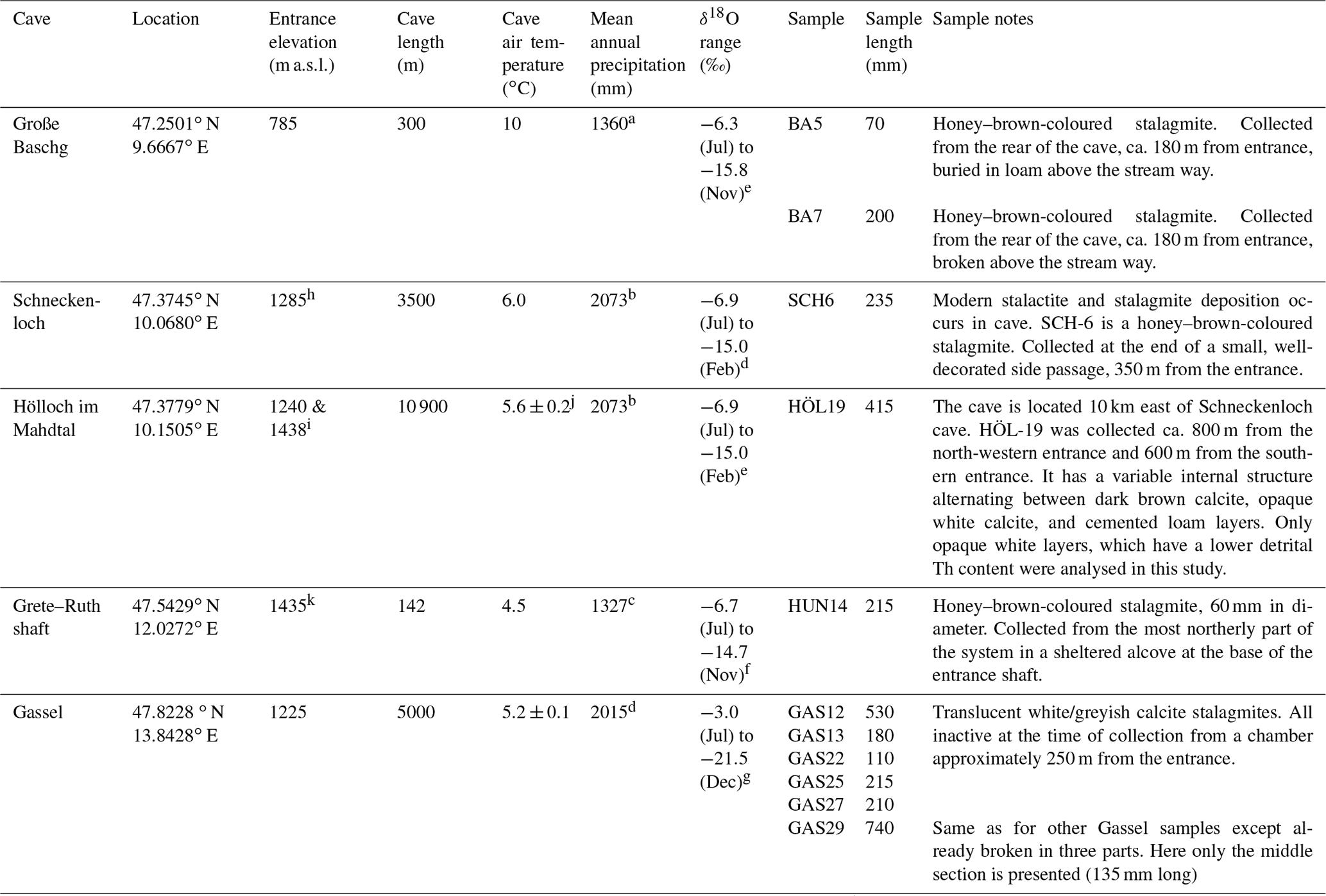
^a Recorded at the Feldkirch meteorological station located ca. 5 km WNW from the cave at 438 m a.s.l. between 1981 and 2010 (ZAMG, 2018). ^b Recorded at the Schoppernau meteorological station located ca.7 km SSW from the cave at 839 m a.s.l. (ZAMG, 2018). ^c Recorded at the Kufstein meteorological station located ca.12 km ENE from the cave at 492 m a.s.l. (ZAMG, 2018). ^d Recorded at the Feuerkogel meteorological station located ca. 10 km west from the cave at 1618 m a.s.l. (ZAMG, 2018). ^e Nearest GNIP station is located 20 km SW at Sevelen (IAEA, 2018). ^d Nearest GNIP station is located 50 km WNW at St. Gallen (IAEA, 2018). ^e Nearest GNIP stations are located ca. 57 km WNW at St. Gallen (−6.9 (Jul) to −15.0 (Feb) ‰) and 70 km ENE at Garmisch–Partenkirchen (−6.7 (Jul) to −14.7 (Nov) ‰; IAEA, 2018). ^f Nearest GNIP station is located 73 km WSW at Garmisch–Partenkirchen (IAEA, 2018). ^g Nearest GNIP station is located 10 km W at Feuerkogel (IAEA, 2018). ^h Klampfer et al. (2017). ⁱ Wolf (2006). ^j Spötl et al. (2011). ^k Rittig (2012).

3 Methods

3.1 Cave sites and speleothems

Previous NALPS studies include MIS 2 in Luetscher et al. (2015; though this was not branded as “NALPS”), MIS 3 in Moseley et al. (2014), and MIS 4 to MIS 5 in Boch et al. (2011). The MIS 4/MIS 5 chronology (which is the part revised here), was constructed from seven speleothems from four cave sites including St. Beatus caves, Große Baschg cave (Baschg cave for short), Klaus Cramer cave and Schneckenloch (Boch et al., 2011). In this study, two additional samples from Baschg cave and one from Schneckenloch were analysed, plus one sample from Hölloch im Mahdtal (Hölloch cave for short), one from Grete–Ruth shaft, and six from Gassel Tropfsteinhöhle (Gassel cave for short). All cave sites are located on the northern rim of the European Alps (Fig. 1) and have small catchments of less than a few square kilometres. The distance between the most westerly and easterly caves is ca. 475 km. Details of the speleothems analysed in this study and their respective caves are given in Table 1, whereas images of the respective samples are given in Fig. S1 in the Supplement.

3.2 Analytical methodology

The 11 stalagmites were cut in half along their growth axis and polished by a professional stone mason. Pilot dating studies guided the sample size that was needed for high precision ages. Sub-samples of between 20 and 150 mg were hand-drilled using a handheld drill fitted with carbide burr-tipped drill bits of diameter 0.5 to 0.8 mm in a laminar-flow hood. The cleanest, densest growth layers were targeted for sampling.

Chemical procedures and aliquot measurements were undertaken in the Trace Metal Isotope Geochemistry Laboratory at the University of Minnesota. Separation and purification of U and Th aliquots from the sub-samples were undertaken using standard methods (Edwards et al., 1987) in a clean air environment. Samples were spiked with a dilute mixed ²²⁹Th-²³³U-²³⁶U tracer to allow for correction of instrumental fractionation and calculation of U and Th concentrations and ratios. Procedural chemistry blanks were on the order of 5–83 ag for ²³⁰Th, 2–523 fg for ²³²Th, 73 to 171 ag for ²³⁴U, and 0.2 to 1.6 pg for ²³⁸U. Aliquots of U and Th were analysed on a Thermo Fisher Neptune multi-collector inductively coupled plasma mass spectrometer (MC-ICPMS) in peak-jumping mode on the secondary electron multiplier (Shen et al., 2012).

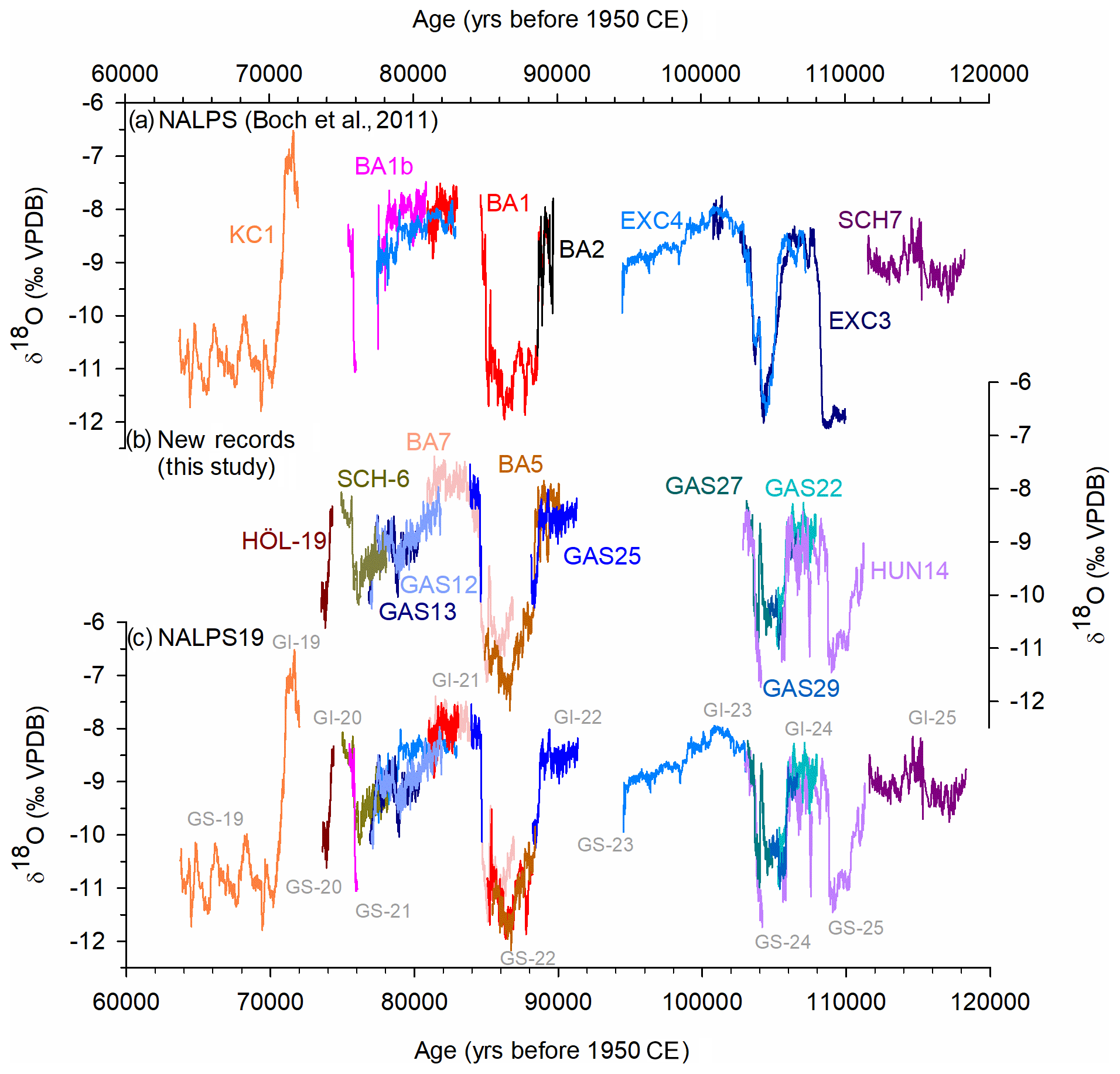
Figure 2 NALPS δ¹⁸O speleothem records (a). Original NALPS record of Boch et al. (2011); (b) new records from this study; (c) the most reliable records of Boch et al. (2011) and this study combined to form NALPS19.

Stable isotopes (δ¹⁸O_calc and δ¹³C_calc) were typically micro-milled at a spatial resolution of 250 µm (with the exception of GAS22 =200 µm and BA7 =500 µm) from the central axis of each sample (Fig. S2). In total 5000 new measurements were made for this study at the University of Innsbruck on a Thermo Fisher Delta^plusXL isotope ratio mass spectrometer linked to a GasBench II. Analytical precisions are 0.08 ‰ and 0.06 ‰ for δ¹⁸O_calc and δ¹³C_calc respectively (1σ; Spötl, 2011). All isotope results are reported relative to the Vienna PeeDee Belemnite standard. In addition to the main isotope track along the central axis, Hendy tests (Hendy, 1971) were also prepared for each sample as a first-order assessment of whether the respective stalagmite was deposited under conditions of isotopic equilibrium, though the preferred approach in recent years has been to reproduce the data in a second stalagmite (Dorale and Liu, 2009). Under the Hendy test criteria, δ¹⁸O_calc values should remain constant along a single growth layer, and there should be no correlation between δ¹⁸O_calc and δ¹³C_calc that might otherwise indicate kinetic fractionation. Bayesian age models were constructed for all 11 samples using OxCal version 4.2 for Poisson-process depositional models (“p sequence”) and a variable “k parameter” of 0.001 to 10 mm a⁻¹ (Bronk Ramsey, 2008; Bronk Ramsey and Lee, 2013).

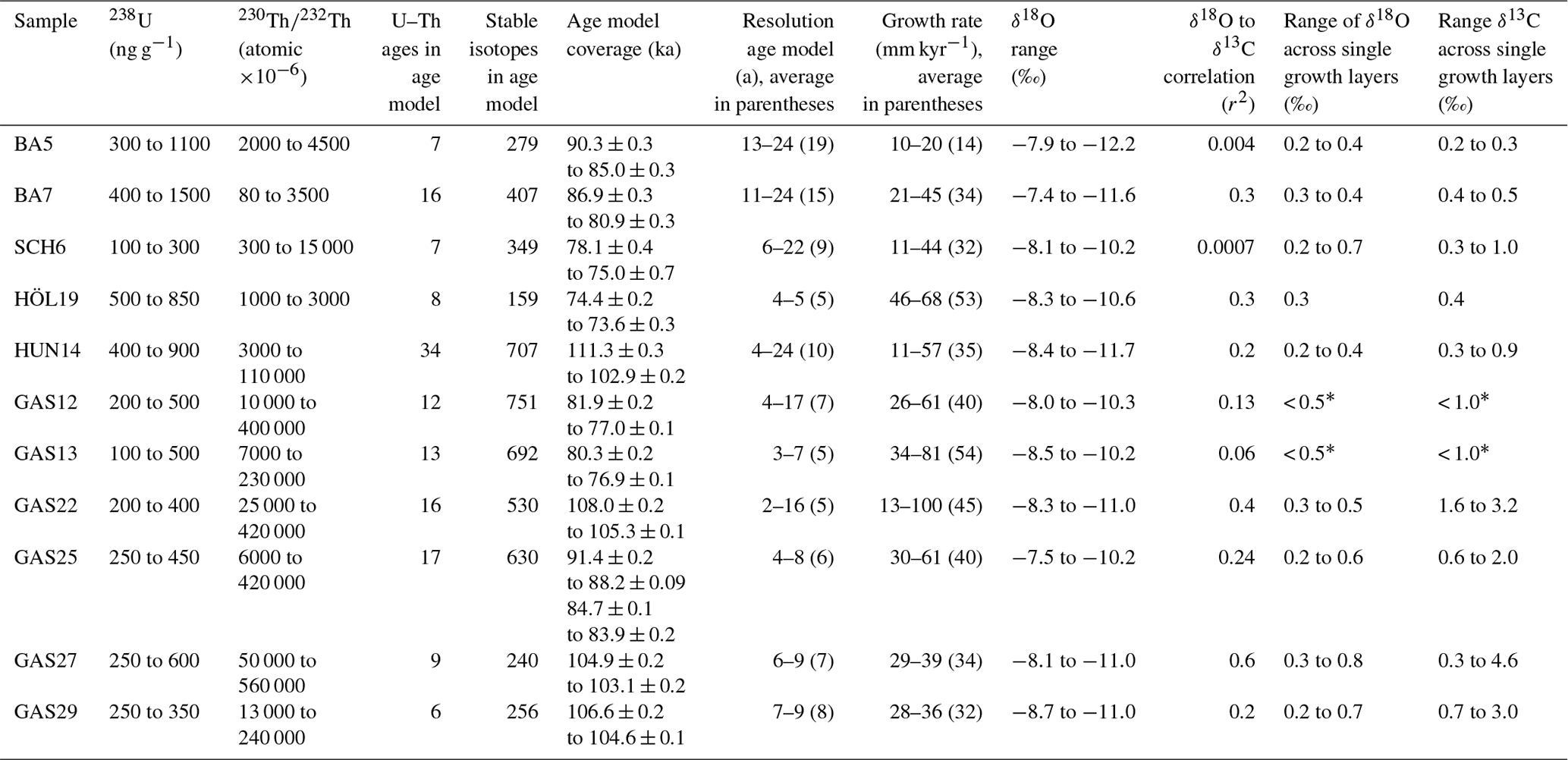
Table 2 Summary of the key features of the U–Th measurements, age modelling, and tests for isotopic equilibrium as presented in Tables S1 and S2, and Figs. S3 and S4.

^* Offenbecher (2004).

4 Results

The results of the U–Th MC-ICPMS measurements and associated age calculations can be found in Table S1 in the Supplement. Age modelling results including growth rates can be seen in Fig. S3. The correlation between δ¹⁸O_calc and δ¹³C_calc is shown in Fig. S4, whereas the results of the Hendy tests are shown in Table S2. The key features of all of these results are summarised in Table 2 and will be discussed briefly here. Generally, all speleothems have ²³⁸U concentrations of ca. 250 to 1500 ng g⁻¹, which are values typical of common alpine dripstones. The cleanest samples, as indicated by high ²³⁰Th∕²³²Th ratios, are from Grete–Ruth shaft (HUN14) and Gassel cave (GAS12, 13, 22, 25, 27, 29). Correction of final ages for detrital Th contamination in these samples is therefore negligible (Table S1). The samples from Baschg, Schneckenloch, and Hölloch caves are all variably contaminated with detrital Th. In the case of BA5, this results in corrections to younger ages of 57–135 years, which are within the levels of dating uncertainty (ca. 300 to 400 years; Table S1). BA-7 is the “dirtiest” of the samples analysed here. Of the 16 U–Th ages used in the age model, 9 are shifted less than 1000 years to younger ages (Table S1). SCH6 has varying levels of detrital Th contamination, being very clean in the older part between 75.9 and 77.9 ka, but moderately dirty in the younger section between 74.4 and 75.5 ka (Table S1). The majority of the age models are thus constructed from clean samples. The internal morphology of HÖL19 is variable and contains sections of clean calcite, dirty calcite, and calcified loam layers (Fig. S1). The youngest part of the stalagmite dates to the late Holocene and the late glacial (Table S1) and thus is outside the time frame for this study. Between ca. 95 and ca. 160 mm from the top, the stalagmite is rich in calcified loam layers and thus is not suitable for dating. Below 160 mm there are a number of sections of clean and dirty calcite. Here we have concentrated on the cleanest part between 187.25 and 226.75 mm from the top. Correction of these ages for detrital Th results in a shift to younger ages of 64 to 213 years, which is within the ca. 300- to 400-year range of dating uncertainty (Table S1). Linear regression analysis between δ¹⁸O_calc and δ¹³C_calc, which is used as a test for isotopic equilibrium (Hendy, 1971; Dorale and Liu, 2009), yields extremely low R² values below 0.3 for the majority of samples (Table 2) suggesting that kinetic fractionation did not occur. Only GAS22 has an R² of 0.4 and GAS27 an R² of 0.6, indicating a minor correlation. Variation in δ¹⁸O_calc across single growth layers is also generally low, with the exception of one out of five tests in GAS27 yielding a range of 0.8 ‰ (Table 2).

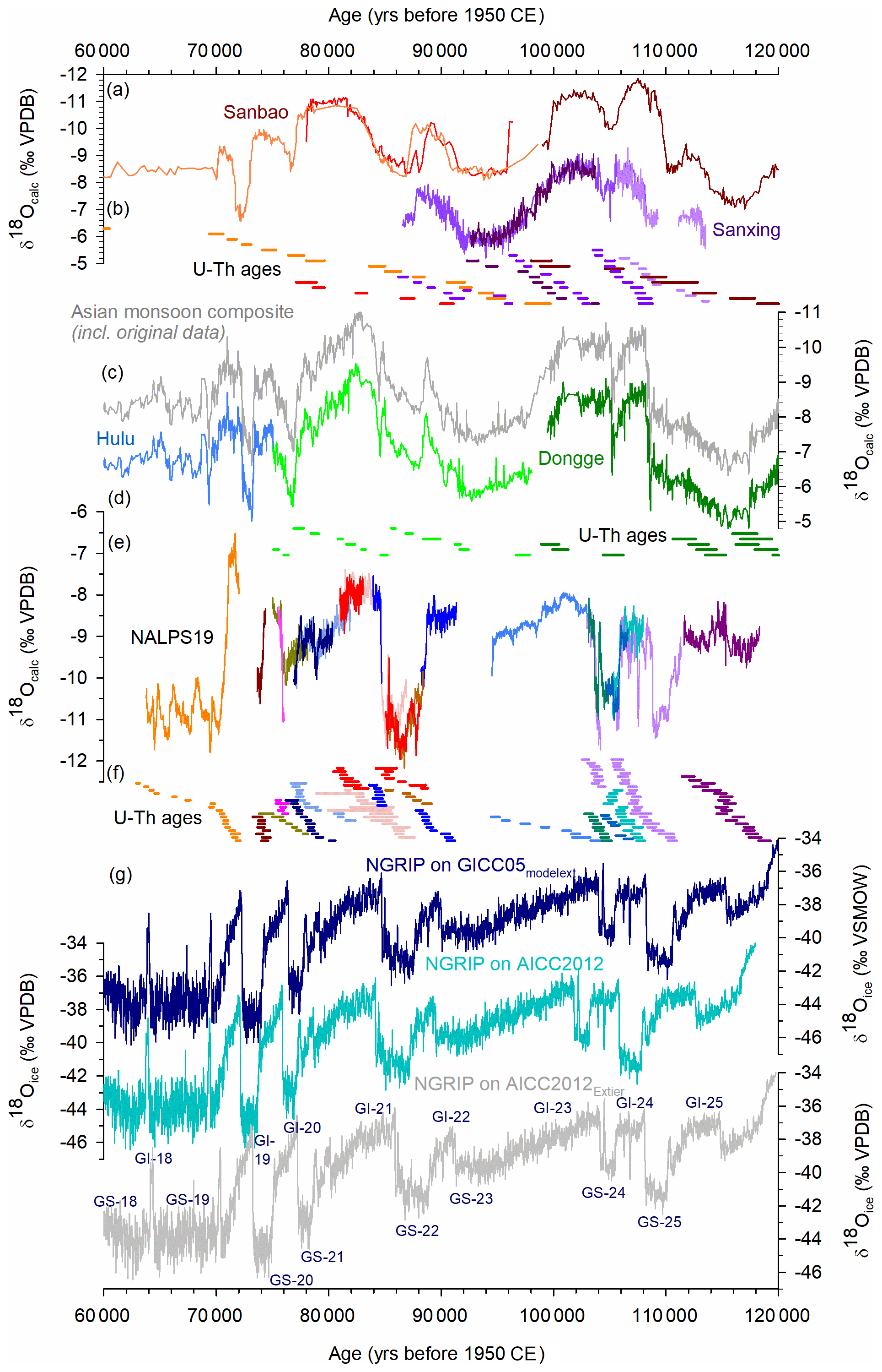
Figure 3 NALPS19 δ¹⁸O record versus other well-dated δ¹⁸O records. (a) Chinese speleothem δ¹⁸O records from Sanbao (Wang et al., 2004) and Sanxing caves (Jiang et al., 2016). (b) 2σ range of U–Th ages used to produce (a) are colour-coded the same as (a). (c) Asian monsoon composite record (Cheng et al., 2016) as well as the original data from which it was constructed (revised Hulu record; Cheng et al., 2016; Dongge; Kelly et al., 2006; Kelly, 2010). In Cheng et al. (2016), the Dongge and Hulu δ¹⁸O values are reduced by 1.6 ‰ in the composite record to match the Sanbao record of Wang et al. (2008). (d) 2σ range of U–Th ages used to produce (c) are colour-coded the same as (c). (e) NALPS19 record (this study). (f) 2σ range of U–Th ages used to produce (e) are colour-coded the same as (e). (g) NGRIP records on the GICC05_modelext chronology (Svensson et al., 2008; Wolff et al., 2010), AICC2012 chronology (Veres et al., 2013), and AICC2012 revised according to Extier et al. (2018). To see this graph split into 20 000-year slices and with the INTIMATE event stratigraphy scheme (Rasmussen et al., 2014), see Fig. S6.

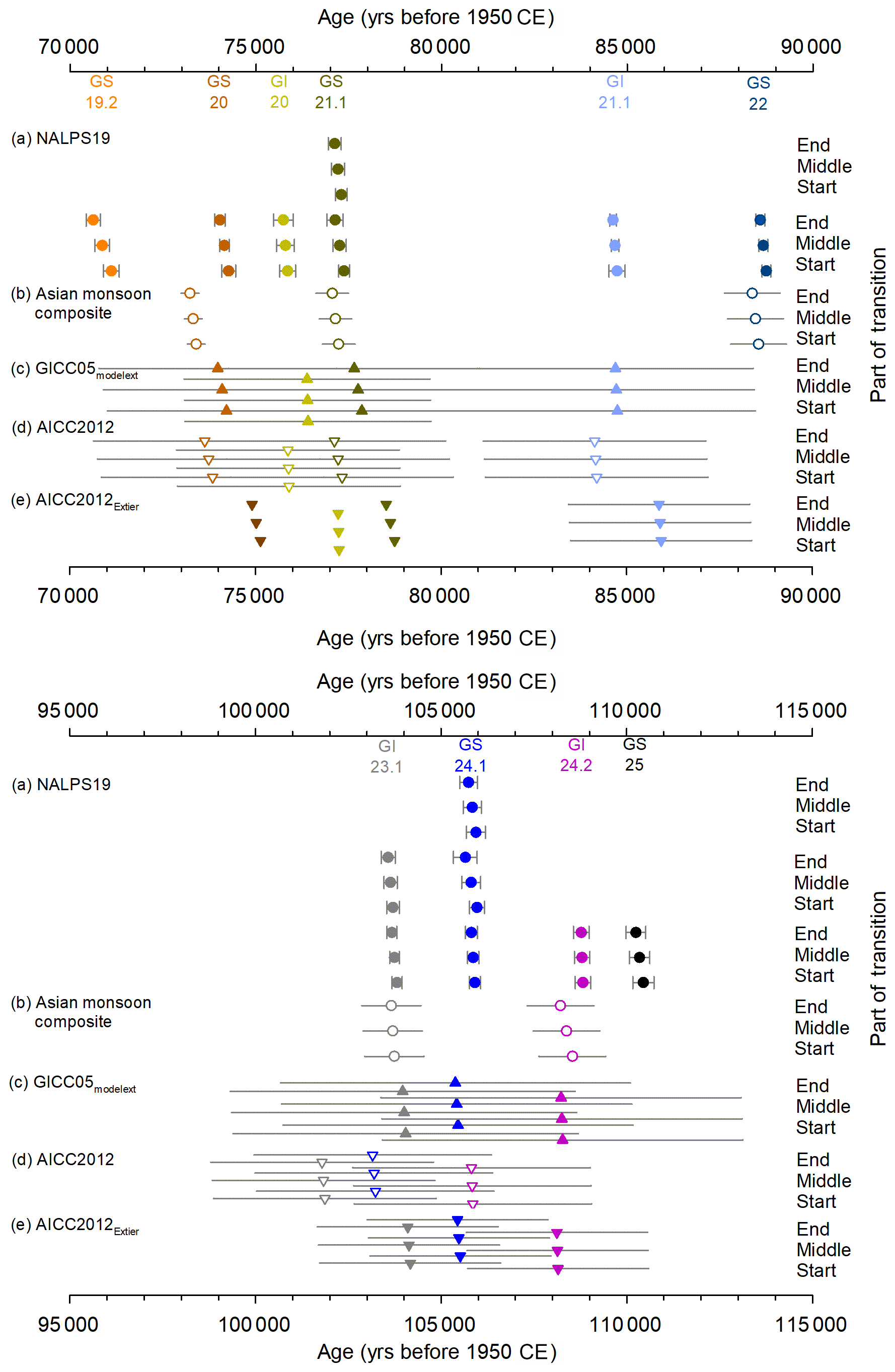
Figure 4 The timing of transitions as defined by the ramp-fitting model of Erhardt et al. (2019). The symbols relate to the age of the start, middle, and end of the transitions as defined by the ramp-fitting, whereas the uncertainty bars are related to the original chronologies. (a) NALPS19 δ¹⁸O_calc record (closed circles; this study); (b) Asian monsoon composite speleothem δ¹⁸O_calc record (open circles; Kelly et al., 2006; Kelly, 2010; Cheng et al., 2016); (c) NGRIP δ¹⁸O_ice record on GICC05_modelext chronology (closed upward triangles; Wolff et al., 2010); (d) NGRIP δ¹⁸O_ice record on AICC2012 chronology (open downward triangles; Veres et al., 2013); NGRIP δ¹⁸O_ice record on the Extier et al. (2018) revised AICC2012 chronology (closed downward triangles). Each ramp fit relative to its reference curve is given in Fig. S7. The GICC05_modelext chronology does not contain uncertainties in this time period (Wolff et al., 2010), and thus these errors are based on the maximum counting error of Svensson et al. (2008). Extier et al. (2018) quote an uncertainty of 2440 years (2σ) in MIS 5. Uncertainties are not given outside of MIS5.

5 Discussion

5.1 Coherence and updates to NALPS19 versus NALPS

The new records produced in this study (Fig. 2b) comprise 5000 δ¹⁸O_calc measurements dated by 145 precise U–Th ages (Fig. S3, Table S1), which add to the NALPS chronology of Boch et al. (2011; Fig. 2a) that comprised 7141 δ¹⁸O_calc measurements and 154 U–Th ages. Combined, the two chronologies cover the period 118.3 to 63.7 ka. Within this interval, the record is now 90 % complete, compared to 76 % in Boch et al. (2011). Where speleothems grew synchronously, major transitional events between stadials and interstadials (and vice versa) are all in agreement within uncertainty, which can be very clearly seen in Fig. S5. In the interest of completeness and transparency, we present all δ¹⁸O_calc records here; however, some samples are cleaner than others as discussed in Sect. 4 (i.e. low in detrital Th as indicated by a higher ²³⁰Th∕²³²Th ratio) and thus deemed to be more reliably dated. The NALPS19 chronology is therefore constructed from only the most reliably dated records from this study and Boch et al. (2011; Fig. 2c). Considering the construction of NALPS19 further and generally working from youngest to oldest, samples KC1 and HÖL19 are included on the basis that they are the only records available that cover the transitions into stadials 19 and 20. The transition into interstadial 20 is present in both SCH6 (this study) and BA1b (Boch et al., 2011). Both samples have comparable levels of detrital Th, and the dating precision of the transition in both samples is ca. 200 to 250 years. Given the comparative cleanliness and dating precision, as well as the reproducibility of the timing of the transition to within ca. 50 to 85 years (Fig. S5), both samples are included in NALPS19. Samples covering the transition into stadial 21 include GAS12 and 13 (this study) and BA1b (Boch et al., 2011). Samples from GAS12 and GAS13 are extremely clean with dating precisions of 250 to 300 years (Table 2), whereas those from BA1b are generally moderate to very clean. Critically though, GAS12 contains six ages and over 60 δ¹⁸O_calc measurements within the transition, and GAS13, three ages and over 130 δ¹⁸O_calc measurements (Fig. S2). On the other hand, BA1b has only three δ¹⁸O_calc measurements in the transition, and one age which is quite dirty resulting in an age corrected to younger values by 760 years and a dating precision of 580 years (Boch et al., 2011). Based on the higher resolution and higher precision provided by GAS12 and GAS13, as well as the fact they are reproducible during the transition on subdecadal and decadal timescales, we therefore include GAS12 and GAS13 in NALPS19 and omit BA1b. EXC4 is then included for the interstadial 21 portion on the basis that it is clean. However, for this section it only contains the interstadial and no transitions, therefore it is excluded from the discussion on transition timing (Sect. 5.2). The transition into interstadial 21 is captured in BA1 (Boch et al., 2011), BA7 and GAS25 (this study). As discussed above, GAS25 is extremely clean, thus correction for detrital Th is negligible and the dating precision is on the order of 300 to 400 years (Table S2). In contrast, BA7 is the dirtiest of the samples with large corrections for detrital Th (Table S1), whereas BA1 is moderately dirty resulting in comparable shifts to younger ages (Boch et al., 2011). Ideally, the complete transition would be constrained only in GAS25 since this sample is the most reliable and best dated, but unfortunately this record is limited to growth mainly during and just after the transition. We therefore include GAS25 where it is applicable and omit BA1 and BA7, but then keep BA1 and BA7 for the parts of the record where there is no alternative available. The transition into stadial 22 is present in GAS25, BA5 (this study), and BA2 (Boch et al., 2011). The situation here is similar to the transition into interstadial 21, where GAS25 is the superior sample with higher dating quality. GAS25 therefore takes priority, whereas BA5 is included to complete the stadial part of the record. BA2 is completely omitted from NALPS19 on the basis that correcting for detrital Th causes shifts in ages in terms of centuries (Boch et al., 2011) as compared to decades in GAS25 (Table S1). The section of the record encompassing interstadial 23, stadial 24, and interstadial 24 is fully covered by GAS22, GAS27, GAS29, and HUN14, which are all extremely clean, well-dated records with typical dating precisions of 300 to 400 years (Table 2). Furthermore, the timing of the transition into interstadial 23 is reproducible to within 60 to 100 years between GAS27 and HUN14. The timing of the transition into stadial 24 is in agreement on the order of 40 to 60 years in GAS22, GAS29, and HUN14. Furthermore, the pattern of δ¹⁸O_calc shifts across the whole interstadial 24 to 23 period is remarkably similar in the new speleothems analysed here to the pattern of events in NGRIP δ¹⁸O_ice across the same period. This suggests the new speleothem samples are capturing a larger-scale climate signal, unlike EXC3 and EXC4 from St. Beatus cave (Boch et al., 2011), which show a distinctly different pattern in δ¹⁸O_calc across this time period. The reason for the difference is unknown, and is likely due to some local influence or control at the cave site. We acknowledge that there is still value in the St. Beatus records, but they are not ideal for investigations into leads, lags, and synchronicity when more comparable records exist; thus they are not included in NALPS19. Finally, the new record from HUN14 is used to complete the gap that existed previously at stadial 25.

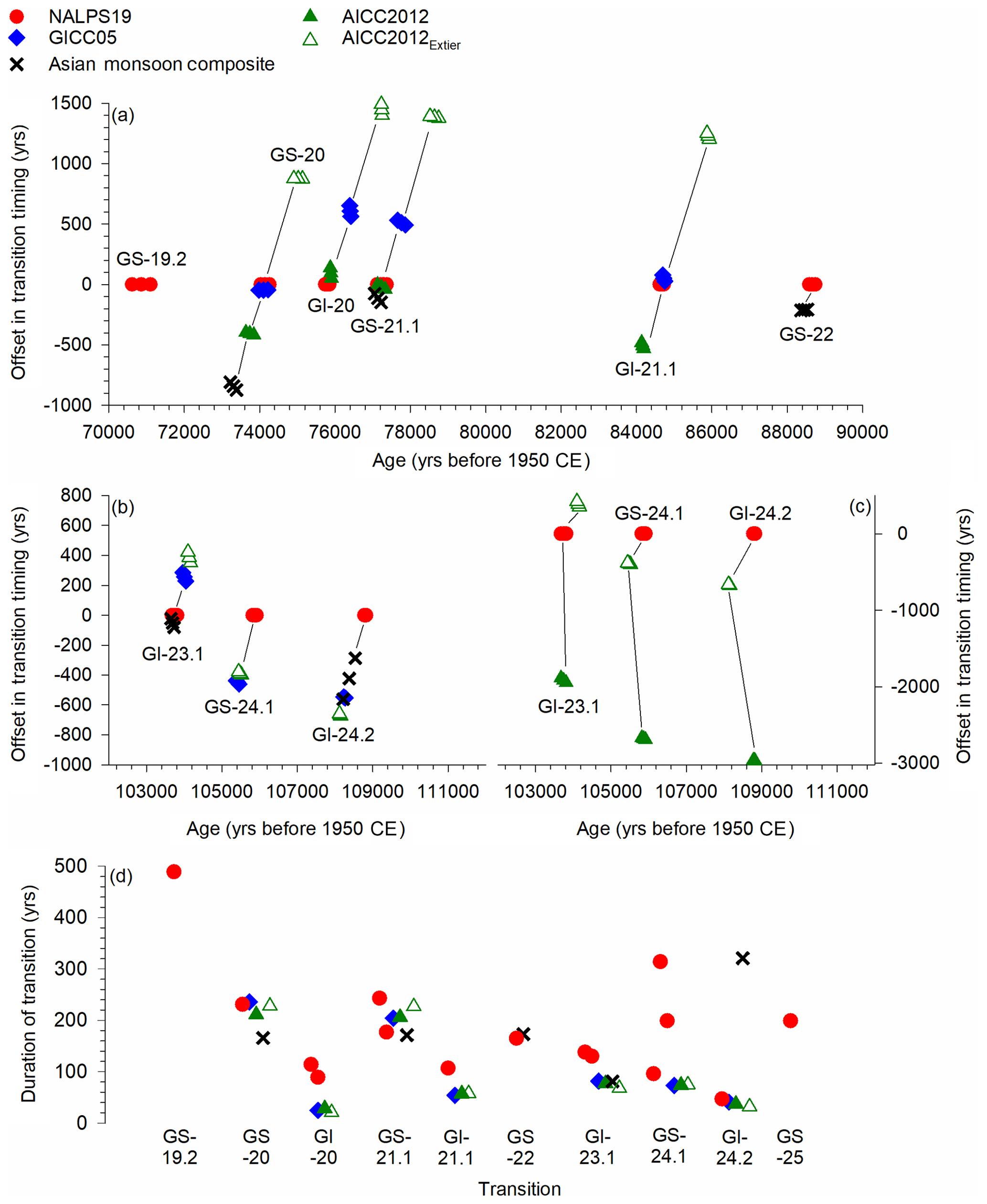
Figure 5 (a, b, c) Offsets in absolute chronology relative to NALPS19 of transitions into stadials and interstadials as defined by the ramp-fitting applied in this study. (+) values indicate the timing in the respective chronology is older/earlier than in NALPS19. (−) values indicate the timing in the respective chronology is younger/later than in NALPS19. Lines are used to indicate the same transition. (d) Duration of transitions. NALPS19 (red circles; this study); NGRIP on GICC05_modelext chronology (blue diamonds; Wolff et al., 2010); NGRIP on AICC2012 chronology (green triangles; Veres et al., 2013); NGRIP on Extier et al. (2018) revised AICC2012 chronology (open green triangles); Asian monsoon composite speleothem (black crosses; Kelly et al., 2006; Kelly, 2010; Cheng et al., 2016).

In summary, important updates in the NALPS19 chronology (Figs. 2 and S6) therefore include (1) the addition of the cooling into GS-20, (2) a revision of the GI-20c/GS-21.1/GI-21.1a period using multiple cleaner samples, (3) revision of the warming into GI-21.1e and cooling into GS-22, also using a cleaner sample, and (4) revision of the interval GI-23.1 to GI-25c, which includes the addition of the previously absent GI-25a and b and a more distinctive “shape” to GS-24 in line with NGRIP.

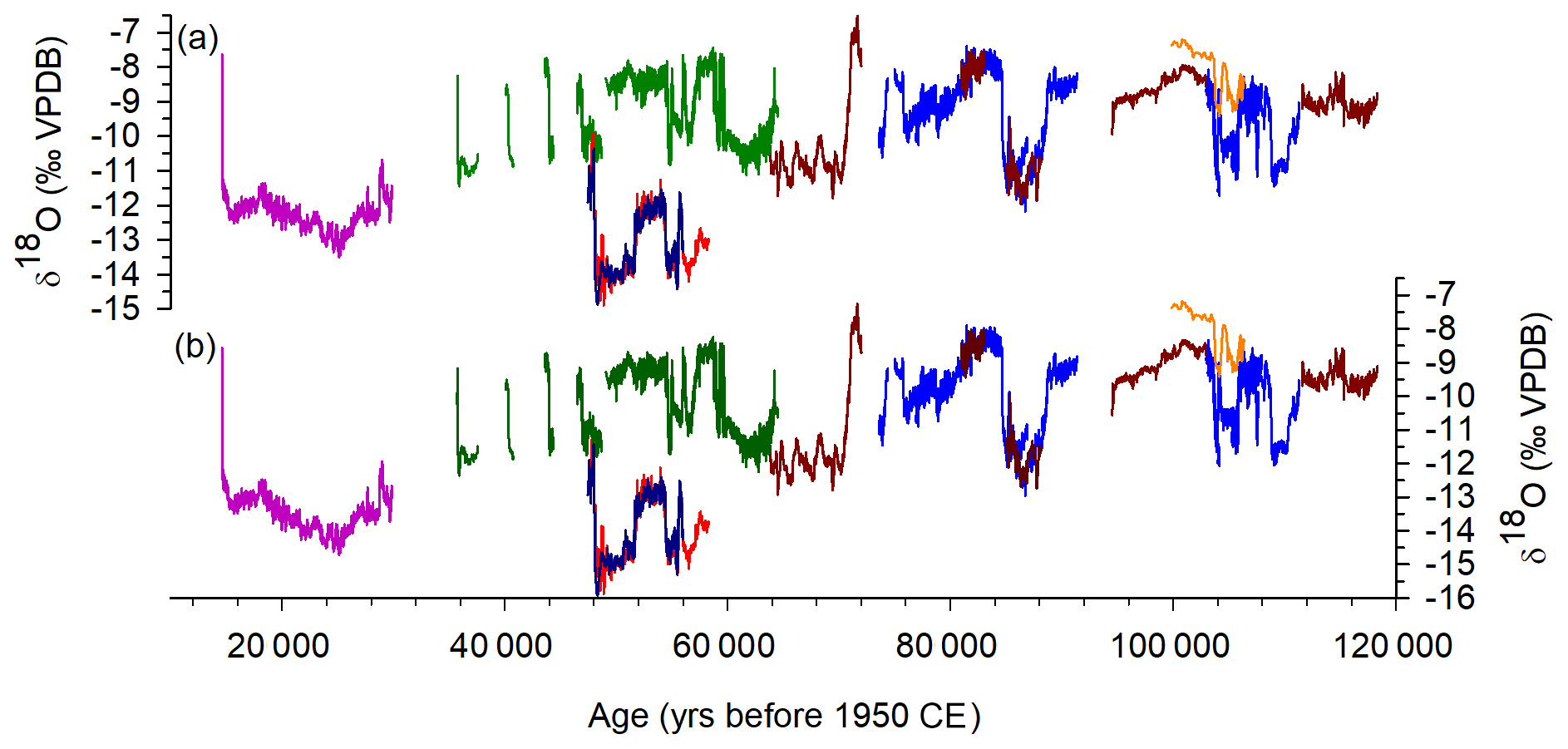
Figure 6 Speleothem δ¹⁸O records from the northern rim and central European Alps. (a) Original records: pink (Luetscher et al., 2015), green (Moseley et al., 2014), red and dark blue (Spötl et al., 2006), dark red (Boch et al., 2011, contained in NALPS19), medium blue (new record in this study), and orange (see Fig. S9). (b) δ¹⁸O records corrected for δ¹⁸O variability as a result of changing ice volume. Colour coding the same as in (a).

5.2 Chronological implications

Figure 3 (split into 20 000-year time slices in Fig. S6) shows the NALPS19 δ¹⁸O_calc record in comparison to other well-dated δ¹⁸O records from distant Northern Hemisphere regions over the interval 60 to 120 ka. Comparison of NGRIP and NALPS19 shows that the broad-scale pattern of shifts in δ¹⁸O was remarkably similar during this period, including down to centennial-scale events. Differences do, however, arise when considering the timing and duration of events, which we investigate further by applying the ramp-fitting function of Erhardt et al. (2019). The ramp-fitting function is similar to the one used by Mudelsee (2000), but instead uses probabilistic inference to define a transition via a linear ramp between two constant levels. Such an approach enables a consistent approach to chronological quantification of climate transitions (Mudelsee, 2000), unlike the more subjective approach of taking the first data point that deviates from the baseline of the previous climate state (e.g. Capron et al., 2010a; Moseley et al., 2014; Rasmussen et al., 2014). Adolphi et al. (2018) applied such a ramp-fitting method to the younger, late glacial portion of the NGRIP δ¹⁸O_ice record (Adolphi et al., 2018), whereas Steffensen et al. (2008) applied another ramp-fitting method through the last deglacial. For this study, ramp-fitting was applied to (1) δ¹⁸O_calc of the new NALPS19 record (this study); (2) δ¹⁸O_calc of the Asian monsoon composite speleothem record (Cheng et al., 2016); (3) NGRIP δ¹⁸O_ice on the GICC05_modelext chronology, which is comprised of a composite layer-counted chronology to 60 ka (Svensson et al., 2008) followed by splicing of the ss09sea-modelled chronology (Johnsen et al., 2001) between 60 and 122 ka onto the younger annual-layer-counted chronology (Wolff et al., 2010); (4) NGRIP δ¹⁸O_ice on the AICC2012 chronology, which is constructed using glaciological inputs, relative and absolute gas and ice stratigraphic markers, and Bayesian modelling (Veres et al., 2013); and (5) NGRIP δ¹⁸O_ice on the AICC2012 chronology updated by aligning δ¹⁸O of the atmosphere as measured in EPICA Dome C with δ¹⁸O_calc of Chinese speleothems (Extier et al., 2018).

Table 3 Results of the ramp-fitting model runs for NALPS19 δ¹⁸O (this study), NGRIP δ¹⁸O on GICC05_modelext (Wolff et al., 2010), NGRIP δ¹⁸O on AICC2012 (Veres et al., 2013), NGRIP δ¹⁸O on AICC2012, revised by Extier et al. (2018), and the Asian monsoon composite δ¹⁸O (Kelly et al., 2006; Kelly, 2010; Cheng et al., 2016). All ages are reported relative to 1950 CE. Uncertainties given are modelling uncertainties as marginal posterior standard deviations. Uncertainties in parentheses are associated uncertainties from the original chronologies.

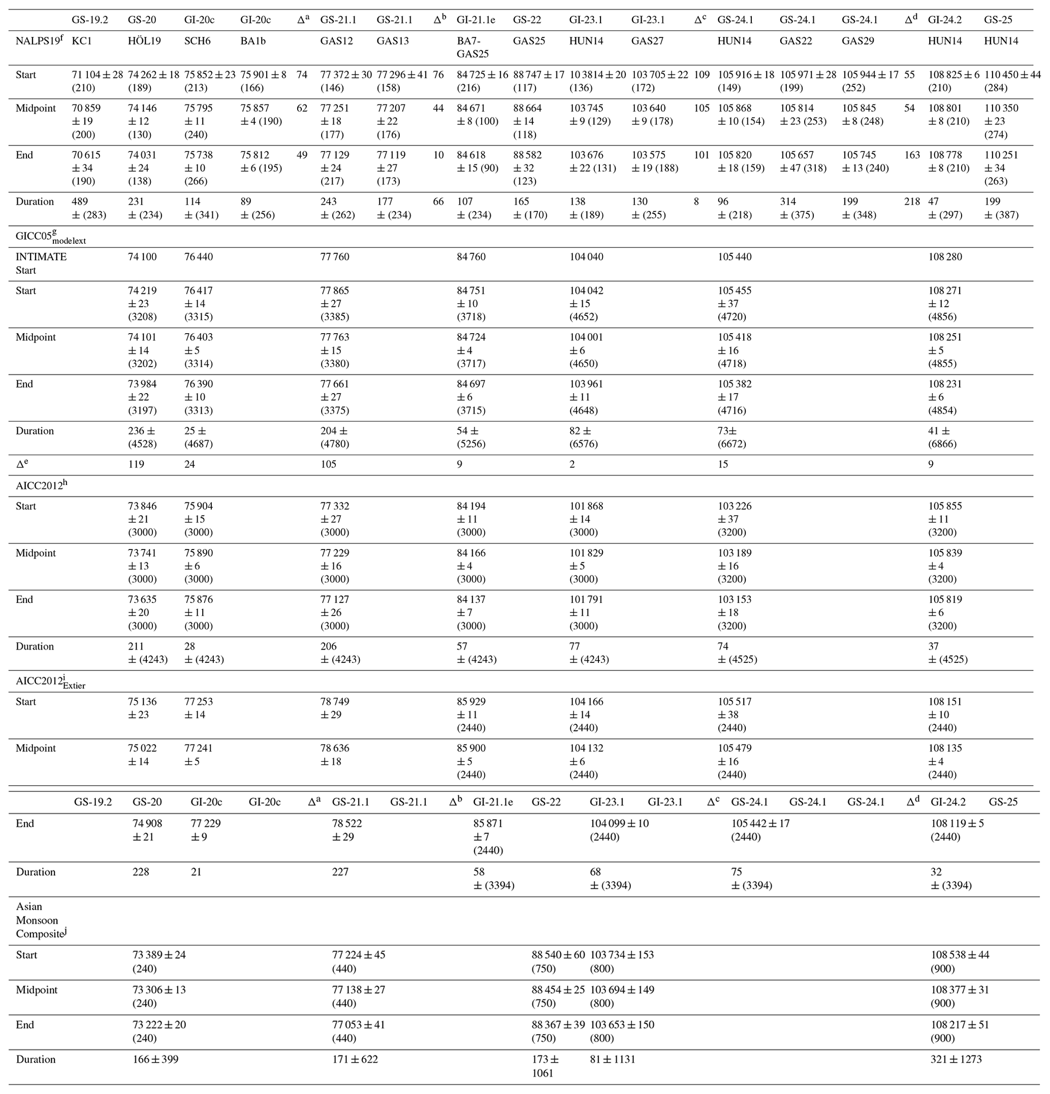
^a Difference in the respective timing between SCH6 and BA1b. ^b Difference in the respective timing between GAS12 and GAS13. ^c Difference in the respective timing between HUN14 and GAS27. ^d Largest difference in the respective timing between HUN14, GAS22, and GAS29. ^e Difference in the respective timing for the start of transitions in GICC05_modelext as defined by the INTIMATE event stratigraphy (Rasmussen et al., 2014) scheme and ramp-fitting (this study). ^f This study. ^g Wolff et al. (2010). ^h Veres et al. (2013). ⁱ Extier et al. (2018). ^j Cheng et al. (2016).

Results of the ramp-fitting are shown in Table 3, Figs. 4 and 5, and S7. Unfortunately, results are not available for some transitions because their shape is incompatible with the transition model, which requires stable periods before and after the transitions. Where multiple NALPS19 speleothems grew synchronously, excellent agreement is found in the absolute timing of the transitions, which shows differences from as little as 10 years between GAS12 and GAS13 during the endpoint of the transition into GS-21.1, up to a maximum of only 163 years difference between GAS22 and HUN14 during the endpoint of the transition into GS-24.1 (i.e. within the 318 years uncertainty of GAS22 at this point; Table 3, Fig. 4). Similarly, for the NGRIP δ¹⁸O_ice record on the GICC05_modelext chronology, we find that the timing of the start of the respective transitions are in excellent agreement (2 to 119 years) between the ramp-fitting used in this study and the INTIMATE event stratigraphy scheme (Rasmussen et al., 2014; Table 3). Comparison between the timing of the ramp-fitted transitions in NALPS19 and the Asian monsoon speleothem records also show excellent agreement within centennial-scale uncertainties, with the exception of GS-20, which is older in NALPS19 by ca. 900 years (Table 3 and Figs. 4 and 5). The NALPS19 age for GS-20 is, however, in very good agreement on a multi-decadal scale with the GICC05_modelext chronology (details below). It should be noted that a comprehensive comparison of the timing of transitions between NALPS19 and NGRIP on the three ice core chronologies is made difficult because of the large uncertainties associated with AICC2012 (ca. 3000–3200 years; Veres et al., 2013) and even the absence of uncertainties associated with GICC05_modelext (Wolff et al., 2010). To deal with the absence of uncertainties in GICC05_modelext, we take the approach of Abbott et al. (2012) and extrapolate the linear trend in ratio between age and uncertainty from the layer-counted 0–60 ka GICC05 chronology (Svensson et al., 2008), which yields an uncertainty of ca. 4.5 % by 120 ka (Table 3, Fig. 4). In reality, the uncertainty is likely to be considerably less since well-dated markers exist in some places (e.g. Guillou et al., 2019). Nevertheless, if only the central age is considered (where + indicates the respective chronology is earlier/older than NALPS19, and − is vice versa), excellent agreement in the absolute timing of the transition is displayed between NALPS19 and GICC05_modelext for GS-20, which is offset by ca. −45 years, and GI-21.1, which is offset by ca. +20 to +80 years (Table 3, Figs. 4 and 5). Depending on the speleothem to which the comparison is made, the transition into GI-23.1 is offset by ca. +230 to +290 years (HUN14) or ca. +340 to +390 years (GAS27). The other transitions into GI-20 (+560 to +650 years), GS-21.1 (+490 to +570 years), GS-24.1 (−440 to −460 years), and GI-24.2 (ca. −550 years) display the largest of the offsets (Table 3 and Figs. 4 and 5). Comparison between NALPS19 and NGRIP on AICC2012 shows good agreement in the timing of GS-21.1 (ca. +8 to −40 years) and GI-20 (+50 to +140 years). The timing for GS-21.1 is further supported in this instance by the close agreement also of the Asian monsoon composite chronology (−70 to −150 years; Fig. 5). Elsewhere, the transitions in the NALPS19 chronology are consistently earlier than their counterparts in the AICC2012 chronology i.e. GS-20 (ca. −400 years), GI-21.1 (ca. −500 years), GI-23.1 (ca. −1900 years), GS-24.1 (ca. −2700 years), and GI-24.2 (ca. −2960 years), suggesting that some revision of the AICC2012 chronology may be needed. Extier et al. (2018) have also proposed such a revision for the period 100 to 120 ka, which is the interval in which there is the greatest discrepancy between AICC2012 and NALPS19. Application of the ramp-fitting to the AICC2012 chronology revised by Extier et al. (2018; AICC2012_Extier) shows that there is much better agreement with NALPS19 during the 100 to 120 ka interval than existed for AICC2012 (Figs. 4 and 5). Specifically, the offset for GI-23.1 is ca. +350 years, GS-24.1 is ca. −400 years, and GI-24.1 is ca. −700 years.

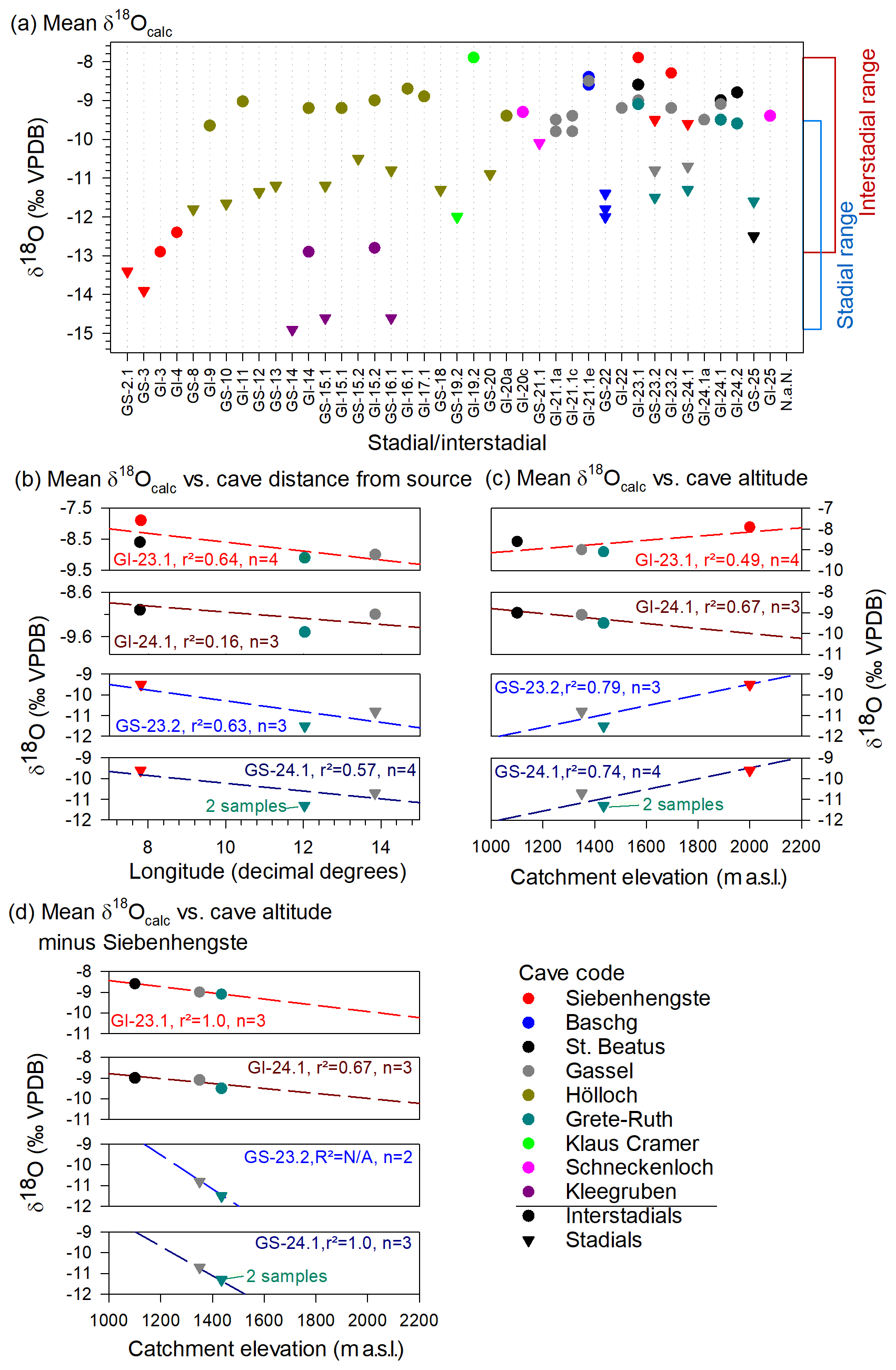
Figure 7 (a) Mean δ¹⁸O_calc for individual caves during specific stadials (triangles) and interstadials (circles). (b) Mean δ¹⁸O_calc values for specific time periods plotted relative to longitude. (c) Mean δ¹⁸O_calc values for specific time periods plotted relative to catchment elevation. (d) Same as (c) minus the data for Siebenhengste.

The ramp-fitted transitions have also enabled an assessment of the duration of δ¹⁸O transitions in the respective chronologies (Table 3, Fig. 5). The quickest shift of 21 years is displayed for the AICC2012_Extier transition into GI-20, whereas the longest shift of 489 years is present in NALPS19 for the transition into GS-19.2. Consistency in the duration of transitions between NALPS19 and the Greenland chronologies is displayed in particular for GS-20 (211 to 236 years), GS-21.1 (204 to 243 years), GS-24.1 (73 to 96 years), and GI-24.2 (32 to 47 years; Table 3, Fig. 5). The difference in durations for GI-21.1 (54 to 107 years) and GI-23.1 (68 to 138 years) is slightly larger but still comparable on multi-decadal timescales. The greatest difference between NALPS19 and the Greenland chronologies is displayed for GI-20, which varies between 21 and 114 years. Interestingly, with the exception of GI-24.2, the duration of transitions in the Asian monsoon are also comparable to the North Atlantic-sourced NALPS19 and Greenland chronologies (on multi-decadal and multi-centennial timescales; Table 3, Fig. 5).

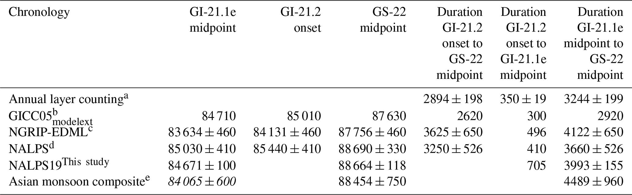
Table 4 The duration of GS-22 and the precursor event (GI-21.2) in various chronologies. All ages given relative to 1950 CE and with 2σ uncertainty.

^a Vallelonga et al. (2012). ^b Wolff et al. (2012). ^c Capron et al. (2010b); Vallelonga et al. (2012). ^d Boch et al. (2011). ^e Cheng et al. (2016) with ramp-fitting from this study. Italics indicates where a transition could not be ramp-fitted and is therefore manually assessed.

The NALPS19 chronology also enables new consideration of the duration of GS-22, which previously has been the subject of debate given the various different timescales presented in the literature (Boch et al., 2011; Vallelonga et al., 2012). Here, we use the same strategy as for the previous studies and define the duration of GS-22 as being from the midpoint of the δ¹⁸O transition into GS-22 until the start of the δ¹⁸O transition into GI-21.2 (Capron et al., 2010a; Vallelonga et al., 2012). The precursor event is defined as the start of the δ¹⁸O transition into GI-21.2 until the midpoint of the δ¹⁸O transition into GI-21.1e. All uncertainties are at the 95 % confidence interval. Based on multi-proxy annual layer-counting, Vallelonga et al. (2012) proposed the duration of GS-22 in the NGRIP ice to be 2894±198 years and the precursor event to be 350±19 years (together 3244±199 years, 2σ error; Table 4). The Vallelonga et al. (2012) layer-counted chronology thus indicated a longer duration for GS-22 than the GICC05_modelext chronology (2620 years) and a shorter duration for the precursor event (300 years, together 2920 years; Table 4; Wolff et al., 2010). The ramp-fitting function was not able to constrain the transition into the precursor event (GI-21.2); thus we consider here the duration of the full period from the cooling into GS-22 to the warming into GI-21.1e, which in the NALPS19 chronology is 3993±155 years (Table 4). This finding is in agreement with the duration from the previous NALPS chronology of 3660±526 years (Table 4), but is ca. 1000 years longer than in GICC05_modelext and 750 years longer than in the layer-counted chronology (395 years if the uncertainties are considered). In contrast, a relatively long duration of 4122±650 years has been proposed for NGRIP on the EPICA Dronning Maud Land (EDML) Antarctic ice core chronology (Capron et al., 2010b; Vallelonga et al., 2012), which is in agreement with the duration from NALPS19. Additionally, the duration of the same period as estimated from the Asian monsoon composite record is 4489±960 years. The speleothem δ¹⁸O_calc records from both the Alps and China therefore support a longer duration for the period between the cooling into GS-22 to the warming into GI-21.1e, which is in line with the NGRIP-EDML chronology (Capron et al., 2010b; Vallelonga et al., 2012).

5.3 NALPS δ¹⁸O variability during the last glacial period (15–120 ka)

Speleothem deposits from the northern rim of the Alps now provide a near-complete record of δ¹⁸O_calc variability during the last glacial period (Fig. 6; Boch et al., 2011; Moseley et al., 2014; Luetscher et al., 2015), which is remarkably similar to δ¹⁸O variability recorded in the NGRIP Greenland ice core during the same period. It is hypothesised that the moisture source for both regions during the last glacial period was the North Atlantic, with the primary control on the δ¹⁸O of precipitation in both Greenland and the Alps being temperature (Boch et al., 2011). Changes to the transport pathway have, however, been proposed for the northern Alpine speleothem record of the Last Glacial Maximum (LGM) between 26.5 and 23.5 ka induced by a southward shift in the North Atlantic storm track (Luetscher et al., 2015). The change to the transport pathway is, however, only considered to affect the LGM and not the remainder of the glacial (Luetscher et al., 2015).

We now consider the full glacial Alpine speleothem δ¹⁸O_calc record in further detail. In addition to the NALPS records of Boch et al. (2011), Moseley et al. (2014) and NALPS19 (this study), we also consider an MIS 5 record from Siebenhengste (Fig. S9), a large cave system located on the northern rim of the Alps of Switzerland (Fig. 1), and a record from Kleegruben cave (Spötl et al., 2006), which is located in the Central Alps of Austria to the north of the main Alpine crest (Fig. 1). A thorough investigation of the controls on the δ¹⁸O of precipitation would require a sophisticated modelling approach, which is beyond the scope of this paper; thus here we appreciate that our investigation is a first consideration only. Furthermore, given the many different factors that can influence the δ¹⁸O of precipitation (Dansgaard, 1964; Rozanski et al., 1993; Clark and Fritz, 1997), it would be advantageous to have stable isotope information from fluid inclusions. Unfortunately, the speleothems presented here are largely devoid of fluid inclusions (Brandstätter, unpublished data).

Figure 8 (a) NGRIP δ¹⁸O_ice on GICC05_modelext (Wolff et al., 2010). (b) NALPS19 δ¹⁸O_calc uncorrected for variability in ocean δ¹⁸O (grey), corrected for variability in ocean δ¹⁸O (black). (c) Growth periods in Brazilian speleothem (dark blue; Wang et al., 2004). Centennial-scale cold reversals of 16.2, 17.2, 21.2, 23.2, and 24.2 are highlighted as vertical dashed yellow bars. (d) Sea-level variability (Grant et al., 2012). Relative sea-level data (grey crosses). Maximum probability relative sea level (grey line). Rate of sea-level change (blue line). Rate of 12 m kyr⁻¹ indicated by horizontal red line. Peaks of sea-level change in excess of 12 m kyr⁻¹ indicated by yellow bars. (e) Ice-rafted debris (dark blue), benthic δ¹³C (green), and planktic δ¹⁸O (orange) from ODP980 on the Hulu U–Th age scale (McManus et al., 1999; Barker et al., 2011).

Today, temperature has been shown to have the most dominant control on the δ¹⁸O of precipitation along the northern rim of the Austrian Alps (Kaiser et al., 2002; Hager and Foelsche, 2015), though other factors such as a changing moisture source, rain-out along the different transport pathways (continental effect), altitude (altitude effect), the North Atlantic Oscillation, and locally also the amount of rain (amount effect) all show some additional control (Ambach et al., 1968; Dray et al., 1998; Kaiser et al., 2002; Hager and Foelsche, 2015; Deininger et al., 2016). To consider the effects of these controls on the δ¹⁸O of precipitation during the last glacial period, we have first removed from the speleothem records the variability in mean ocean δ¹⁸O caused by fluctuations in ice volume (Fig. 6) using a rate of 0.012 ‰ m⁻¹ (Rohling, 2013) and the sea-level curve of Grant et al. (2012).

Mean speleothem δ¹⁸O_calc values for individual stadials and interstadials in the ice-volume-corrected record have been calculated for each sample (Figs. 7a, S8, Table S3). Excluding the samples associated with the LGM because of the different transport pathway (Luetscher et al., 2015), the δ¹⁸O_calc range in mean interstadial values is 5.0 ‰ (Klaus Cramer (−7.9 ‰) and Siebenhengste (−7.9 ‰) to Kleegruben (−12.9 ‰), whilst the range in mean δ¹⁸O_calc stadial values is slightly larger (but comparable) at 5.4 ‰ (Siebenhengste (−9.5 ‰) to Kleegruben (−14.9 ‰); Fig. 7a). We now consider the controls on δ¹⁸O_calc during periods when more than one speleothem was deposited, specifically GI-23.1, GS-23.2, GI-24.1, and GS-24.1. Generally it is considered that the dominant control on the δ¹⁸O of precipitation in the northern and central Alps during the last glacial period was temperature, and the dominant moisture source was the North Atlantic (as both are today). The correlation between both temperature and distance from the North Atlantic as compared to mean δ¹⁸O_calc was investigated to identify potential continental and rainout effects. In all instances, mean δ¹⁸O_calc became increasingly lighter with increasing distance from the North Atlantic; a medium correlation is displayed for GI-23.1 (r²=0.64, n=4), GS-23.2 (r²=0.63, n=3), GS-24.1 (r²=0.57, n=4, two samples for Gassel), and a lower correlation during GI-24.1 (r²=0.16, n=3). This trend of lighter mean δ¹⁸O_calc with increasing distance from the source would be expected with progressive rainout and is consistent with present-day observations.

Today, spatial variability of the δ¹⁸O of precipitation in the Austrian Alps is highly dependent on altitude (Hager and Foelsche, 2015). We find that medium to strong correlations between catchment elevation and mean δ¹⁸O_calc existed during GI-23.1 (r²=0.49, n=4), GI-24.1 (r²=0.67, n=3), GS-23.2 (r²=0.79 n=3), and GS-24.1 (r²=0.74, n=4 (Gassel has two samples); (Fig. 7c)). For GI-24.1, the relationship shows that mean δ¹⁸O_calc becomes increasingly lighter with increasing elevation (as would be expected for altitudinal controls on δ¹⁸O of precipitation). In contrast, the other examined time periods show an inverse relationship to what would be expected for altitudinal control, with mean δ¹⁸O_calc becoming heavier with increasing elevation (Fig. 7c). Since GI-24.1 is the only event that does not include the high-elevation Siebenhengste site, the mean δ¹⁸O_calc of 7H-12 was removed from the linear regression analysis for the three time periods showing an inverse relationship (Fig. 7d). This resulted in a switch to increasingly lighter mean δ¹⁸O_calc with increasing elevation for GI-23.1, GS-23.2, and GS-24.1 (Fig. 7d; i.e. in line with an altitudinal control on δ¹⁸O of precipitation).

Given that there is such limited availability of multiple speleothem δ¹⁸O records covering the same time periods, it is difficult to make firm conclusions on the controls of δ¹⁸O_calc. Here though we offer some hypotheses based on the available data. We have shown that for a given time period δ¹⁸O_calc trends towards lighter values with increasing distance from the North Atlantic (Fig. 7b). Despite this, there is some variability overprinted on top of this trend. For instance, even though Grete–Ruth is closer to the North Atlantic than Gassel cave, mean δ¹⁸O_calc values for Grete–Ruth are consistently lighter than for Gassel (Fig. 7b). Since Grete–Ruth is located at a higher elevation than Gassel cave (Fig. 7c), the lighter mean δ¹⁸O_calc values are likely a product of the altitude effect and associated cooler temperatures. In comparison, St. Beatus and Siebenhengste caves are located within 10 km of one another, and are the closest caves to the North Atlantic of all the caves investigated here. As expected, mean δ¹⁸O_calc values are heavier for St. Beatus and Siebenhengste than for Grete–Ruth and Gassel caves (Fig. 7b). Closer investigation, however, shows that during GI-23.1, mean δ¹⁸O_calc of low-elevation St. Beatus is lighter than the high-elevation Siebenhengste (Fig. 7b). Given the close proximity of the two caves, the condensation level (and therefore condensation temperature) would have been approximately the same, and thus one must consider the reason for the difference in mean δ¹⁸O_calc for these two caves. Since the three caves at lower elevation (St. Beatus, Gassel, Grete–Ruth) follow the expected altitude-induced trend of lighter mean δ¹⁸O_calc with increasing elevation (Fig. 7d), it seems the anomaly lies with the high-elevation 7H-12 stalagmite from Siebenhengste. One reason for the heavier-than-expected mean δ¹⁸O_calc at Siebenhengste could be that the full annual signal is better preserved at high-elevation sites that are less exposed to evapotranspiration effects during the summer season than in more vegetated catchments. Alternatively, a summer bias towards isotopically heavier δ¹⁸O_calc at the high-elevation site could for instance be caused by wind erosion resulting in relocation of the isotopically light winter snow, a process that has been well documented at various Alpine sites (Ambach et al., 1968; Bohleber et al., 2013; Hürkamp et al., 2019). Eventually, if firn developed above Siebenhengste during GI-23.1, then this would also limit the input of isotopically light precipitation causing a summer bias in the recorded signal. At present there is, however, no evidence to either support or reject the hypothesis of firn above Siebenhengste during MIS 5.

In summary, speleothems from the northern rim of the European Alps provide δ¹⁸O_calc records for the majority of the last glacial period. As expected, the limited data set shows that mean δ¹⁸O_calc for specific stadials and interstadials generally trends towards lighter values with increasing distance from the coast and with increasing altitude. An exception is the high-elevation 7H-12 stalagmite from Siebenhengste, which appears to record a stronger summer signal. Further investigation of the controls on δ¹⁸O_calc in the northern Alps requires a more sophisticated modelling approach.

5.4 Stadial-level centennial-scale cold events

The recognition of centennial- to millennial-scale climate events, such as precursors to interstadials and “within-interstadial” depletions in δ¹⁸O_ice (Capron et al., 2010a), led to the designation of the INTIMATE event stratigraphy for the Greenland ice cores over the last glacial period (Rasmussen et al., 2014). Typically, a precursor event is a feature of a stadial–interstadial transition; this includes GS-16.2, 17.2, 21.2, and 23.2 (Fig. 8; Capron et al., 2010a; Rasmussen et al., 2014). It is characterised in northern Alpine speleothems and Greenland ice cores by a rapid increase in δ¹⁸O from stadial to interstadial conditions. The event is short lived, lasting a maximum of a few centuries before δ¹⁸O returns to near-stadial conditions for another few decades to centuries, followed by the main transition into the interstadial. [Ca²⁺] in the Greenland ice cores varies almost simultaneously with these δ¹⁸O_ice changes, where increases in [Ca²⁺] are associated with depletions in δ¹⁸O_ice and vice versa. Changes in [Ca²⁺] are interpreted to reflect changes in dust concentration caused by changes in dust source conditions and transport pathways indicative of regional- to hemispheric-scale circulation changes (Ruth et al., 2007). In comparison, within-interstadial climate perturbations are characterised in general by smaller-amplitude depletions in δ¹⁸O_ice that typically do not reach stadial values, and are often of shorter duration than the reversals at stadial–interstadial transitions. [Ca²⁺] also varies in tune with within-interstadial δ¹⁸O_ice fluctuations, but similarly does not reach full stadial values. Such characteristics appear to be consistent in δ¹⁸O records from both Greenland ice cores and northern Alpine speleothems. The exception to such typical within-interstadial cold perturbations is the event at 107.5 ka in the NALPS19 chronology, which is designated GS-24.2 in the INTIMATE event stratigraphy scheme (Rasmussen et al., 2014). This drop in δ¹⁸O_calc to stadial values occurred 978 years after the start of the interstadial, thus firmly making it a within-interstadial event rather than one associated with a stadial–interstadial transition. At present, the 107.5 ka event (GS-24.2) is the only centennial-scale δ¹⁸O event of such extreme amplitude occurring during an interstadial that is recognised in both Greenland and northern Alpine records. Because of this, it has been likened to the 8.2 ka cold event that occurred in the early Holocene (Alley et al., 1997; Capron et al., 2010a). Still, the δ¹⁸O_ice excursion of the 8.2 ka event did not reach near-stadial values in NGRIP as GS-24.2 did, thus highlighting some differences between these two warm-interrupting cold reversals. In addition, Rasmussen et al. (2014) liken the within-interstadial GS-24.2 cold perturbation to stadial–interstadial transition events GS-16.2 and GS-17.2. Both the similarities between GS-24.2 and the 8.2 ka event and those of GS-16.2 and GS-17.2 suggest that such abrupt climate variability is not critically influenced by the size of the Greenland ice sheet (Capron et al., 2010a; Rasmussen et al., 2014).

During the deglacial and early Holocene, large-scale meltwater events are widely suggested as being responsible for causing some short-term climate reversals through the weakening of Atlantic meridional overturning circulation (AMOC; e.g. Broecker, 1994; Teller et al., 2002; Clark et al., 2001). Such cold reversals thought to be triggered by meltwater events include the Older Dryas at 14 ka (GI-1d, Rasmussen et al., 2014), the Preboreal Oscillation at 11.4 ka (e.g. Johnsen et al., 1992; Björck et al., 1996; Fischer et al., 2002), the 9.3 ka event (Fleitmann et al., 2008; Yu et al., 2010), and the 8.2 ka event (Alley et al., 1997). In contrast, however, not all freshwater injections led to cold events, and not all cold events were caused by freshwater injections (Stanford et al., 2006). For instance, both the Younger Dryas and Heinrich events occurred during times of already-colder sea surface temperatures and weakened AMOC, indicating that the input of freshwater from the iceberg armadas was not the initial cause of the AMOC slowdown (e.g. Hall et al., 2006; Henry et al., 2016).

In the case of the centennial-scale cold reversals of GS-16.2, GS-17.2, GS-21.2, GS-23.2, and GS-24.2 (Fig. 8), a possible mechanism for each of these events could be similar to the meltwater-triggered cold reversals of the deglacial. This hypothesis is supported when considering that events GS-17.2, GS-21.2, and GS-24.2 occurred shortly following episodes of rapid sea-level rise, which were in excess of 12 m kyr⁻¹ in the high-resolution record of Grant et al. (2012; Fig. 8). Such rapid sea-level rise does not appear to have occurred prior to GS-23.2, though closer inspection of the sea-level curve shows that following the rise prior to GS-24.2, sea levels had remained elevated and underwent a series of rapid oscillations that are smoothed out in the rate-of-change curve (Fig. 8). Likewise, GS-16.2 did not occur coincident with an episode of sea-level rise, but did occur shortly after the rise associated with GS-17.2 (Fig. 8). Additionally, the rapid rises in sea level each began at times of increased ice-rafted debris (IRD) in the North Atlantic (McManus et al., 1999, on U–Th timescale), weakened AMOC, and increased ice volume as indicated by high benthic δ¹³C and planktic δ¹⁸O values, respectively, as well as pluvial periods in Brazil caused by a southward shift of the intertropical convergence zone (ITCZ; Wang et al., 2004; Fig. 8). In the late glacial, such episodes are associated with Heinrich events (Wang et al., 2004). Furthermore during glacial terminations, the sequence of events has been shown to include a Heinrich event, followed by short-lived warming, and then a millennial-scale return to cold conditions, and finally the transition to the interglacial (Cheng et al., 2009). Though on shorter timescales, the pattern of events during these specific stadial–interstadial transitions is similar to the pattern of events during glacial terminations. The oscillations of GS-16.2, GS-17.2, GS-21.2, and GS-23.2 at stadial–interstadial transitions can therefore be considered as being akin to the meltwater-triggered Preboreal Oscillation, which occurred shortly following the warming at the end of the Younger Dryas stadial during a time when considerable volumes of ice still existed, similar to the early glacial. These reversals at stadial–interstadial transitions during the early glacial period are therefore not so much warming events that punctuate cold periods (Capron et al., 2010a), but rather stadial–interstadial transitions that failed due to freshwater influx. On the other hand, GS-24.2, which occurred nearly 1000 years after warming occurred, is more similar to the Older Dryas in which a cold event punctuated a warm interval.

6 Conclusions

In this paper, we present the most recent chronology, named NALPS19, for δ¹⁸O_calc variability as recorded in speleothems that grew during the last glacial period between ca. 15 and 120 ka along the northern rim of the Alps. In particular, we have updated the record between 63.7 and 118.3 ka, using 11 cleaner and more accurately and precisely dated samples from five caves. Over the 63.7 to 118.3 ka interval, the record is now 90 % complete. Ramp-fitting analysis of the transitions between stadials and interstadials shows that δ¹⁸O shifts in the North Atlantic realm and Asian monsoon occurred on multi-decadal to multi-centennial timescales. Further, the absolute timing of shifts show good agreement between NALPS19 and Greenland ice core chronologies within the multi-millennial-scale ice core uncertainties, though absolute offsets are often on multi-decadal to multi-centennial scales. Major differences do, however, arise when comparing NALPS to NGRIP on AICC2012 between 100 and 120 ka, suggesting that the AICC2012 chronology is too young by ca. 3000 years in this time period. Additionally, we propose that the duration of the highly debated GS-22–GI-21.2–GS-21.2 interval was 3993±155 years, which is in closer agreement with the duration of 4122±650 years in NGRIP-EDML (Capron et al., 2010b) and the 4489±960 years of the Asian monsoon composite record (Kelly et al., 2006; Kelly, 2010; Cheng et al., 2016). Preliminary investigation of the trends in mean δ¹⁸O_calc as recorded in the NALPS speleothems for different interstadials and stadials reveals that for a given time period, as expected, δ¹⁸O_calc becomes lighter with increasing distance from the source and increasing elevation. Exceptions are found at one high-elevation site, which appears to record a stronger summer signal. Finally, our accurate and precise chronology enables deeper investigation of centennial-scale cold reversals that occurred either as precursor events (i.e. GS-16.2, GS-17.2, GS-21.2, GS-23.2; Capron et al., 2010a) or during interstadials (i.e. GS-24.2). Each of these events occurred in the decades and centuries following rapid rises in sea level of over 12 m kyr⁻¹ (Grant et al., 2012) that occurred coincident with IRD events (McManus et al., 1999) and shifts in the ITCZ causing speleothem growth in Brazil (Wang et al., 2004). We therefore propose that these centennial-scale cold reversals are products of freshwater discharge into the North Atlantic during times of moderate ice sheet size, which caused a slowdown of the AMOC and associated atmospheric cooling, similar to deglacial events such as the Preboreal Oscillation or Older Dryas.