Synthetic weather diaries: concept and application to Swiss weather in 1816

Climate science is about to produce numerical daily weather reconstructions based on meteorological measurements for central Europe 250 years back. Using a pilot reconstruction covering Switzerland at a 2×2 km² resolution for 1816, this paper presents methods to translate numerical reconstructions and derived indices into text describing daily weather and the state of vegetation. This facilitates comparison with historical sources and analyses of the effects of weather on different aspects of life. The translation, termed “synthetic weather diary”, could possibly be used to train machine learning approaches to do the reverse: reconstruct past weather from categorised text entries in diaries.

1 Introduction

The past decade has seen tremendous advances in numerical weather reconstructions. They were enabled by new numerical techniques such as data assimilation (Compo et al., 2011), combined with a new demand arising from new scientific questions (better understanding variability), new societal needs (prepare for extreme weather events in the future), and the more widespread use of numerical modelling in climate impact research. In this situation, historical instrumental data – but also documentary weather data – become once again valuable for science (Allan et al., 2011). Based on digitised historical instrumental data, model chains can be built (e.g. numerically simulating the damage of past storm or flood events; see Stucki et al., 2015, 2018) and analysed together with historical sources (e.g. Allan et al., 2016; Veale et al., 2017).

In addition to data assimilation, providing global weather data at a coarse resolution back to the early 19th century (Slivinski et al., 2019), other techniques such as analogue resampling of regional weather fields (Caillouet et al., 2019; Devers et al., 2020; Pfister et al., 2020) have also been used to reconstruct local daily weather 150–200 years back in time, with the potential to go even further back. These reconstructions provide a resource not just for climate science but also for historians. Depending on the application, a translation between numerical weather data and the descriptive text format in which historical observations and weather diaries are typically written would be beneficial. In this paper I present a first step in this direction, termed “synthetic weather diary”.

Turned into categorised text, numerical weather reconstructions could supplement historical sources with weather descriptions, much like weather reports today. They could provide, for instance, information on the day-to-day weather for a specific journey or during a military operation. In addition to the individual measurements, useful information for historians could be gained from specific indices based on these daily data. Such indices could provide information on the freezing of water bodies, the state of vegetation, or drought conditions.

The translation makes numerical reconstructions and observations directly comparable, which is not only useful for historians but also for climate science. For instance, generating synthetic weather diaries from numerical data in recent decades could be used to train machine learning algorithms to provide the weather pattern (e.g. the weather type or even a full spatial field). A trained algorithm could then be used to classify daily weather in the past based on categorised information from historical weather diaries.

The codification of descriptive weather information is a core work of historians of climate (Riemann et al., 2015). A next step is then to establish an ordinal scale, which has been attempted mostly at the monthly or seasonal scale. So-called “Pfister indices” (Pfister et al., 2018) are often used and categorise weather in three-point (−1, 0, 1) or seven-point (−3, −2, −1, 0, 1, 2, 3) indices, with corresponding designations such as “extremely cold” and “cold” (Pfister, 1999). Calibrating such indices with measurement-based time series in order to calibrate climate reconstructions implies a similar translation from numerical data to text, though on the monthly or seasonal scale.

In this paper I describe a pilot study to generate synthetic weather diaries based on daily weather reconstructions for Switzerland for the year 1816, known as a Year Without a Summer. Weather and climate during this year were affected by the eruption of Tambora in Indonesia in 1815 (Raible et al., 2016; Brönnimann and Krämer, 2016). The summer was very cold and rainy, particularly in central Europe (Auchmann et al., 2012; Luterbacher and Pfister, 2015; Veale and Endfield, 2016), although the adverse weather conditions were only partly due to the direct effects of the eruption. The Year Without a Summer of 1816 is arguably among the most prominent climate events of the past few hundred years. Concurring with increased vulnerability after the Napoleonic wars (due to political instability, economic shifts after the end of the continental system, high unemployment rates, and inadequate governance), the societal consequences of this weather event were severe, particularly in Switzerland (Krämer, 2015; Behringer, 2016). Further weather-related effects were linked to snow accumulation, such as avalanches in the following winter (Rohr, 2015) and a flood event in early summer 1817, although the snowmelt contribution was large only close to the Alps (Rössler and Brönnimann, 2018). The Tambora eruption was one of at least five large eruptions within a relatively short period, which together had profound effects on the global climate system, including monsoons, and on Alpine glaciers (Brönnimann et al., 2019a).

In the following I describe the weather reconstruction, the translation into text as well as the generation of impact-related indices. Then I evaluate the synthetic diaries by comparison with daily observations (which are already in categorised form) and monthly weather summaries as well as brief daily weather notes written down on Lord Byron's famous journey through Switzerland (Byron, 1839) in September 1816. A discussion then follows on the use of synthetic weather diaries in history and science. The paper ends with brief conclusions.

2 Data

2.1 Numerical reconstructions

The daily weather reconstructions for 1816 used in this paper are taken from Flückiger et al. (2017) and cover Switzerland. They were produced with the specific aim of numerically modelling potential harvest yields during the Year Without a Summer of 1816 in Switzerland. Furthermore, they were subsequently used to numerically model the flood events of 1817 (Rössler and Brönnimann, 2018). In the following, I give a brief summary of the reconstruction technique. Note that the reconstruction was not designed for day-to-day accuracy. Nevertheless, it best serves the purpose of presenting the concept of synthetic weather diaries as it is the earliest, high-resolution spatial weather reconstruction available at the moment of writing and also because the Year Without a Summer of 1816 is well documented and of particular interest.

The reconstruction is based on an analogue resampling. The analogue pool consists of 59 years of daily 2×2 km² resolved fields of minimum and maximum temperature (T_min and T_max, which we averaged to daily mean temperature, T_mean, for this study) and precipitation from the data sets TminD, TmaxD, and RhiresD (Frei, 2014), reaching back to 1961. Solar irradiance fields were produced using a k nearest-neighbour interpolation. From this pool, the day that is closest to a historical target day, according to all measurements available at that historical day, was chosen, as is detailed in the following. The process was repeated for each day, and the sequence of closest analogues constitutes the reconstruction.

Three stations were used to define a measure of distance between analogue pool and historical target day: Geneva, Delémont (both in Switzerland), and Hohenpeissenberg (Bavaria). These were the only three stations within or in the vicinity of Switzerland with daily or subdaily data at the time the reconstruction was produced. We used T_min and T_max for Geneva and Hohenpeissenberg, T_mean for Delémont, and precipitation for Geneva. The Euclidian distance was chosen as the distance measure. We accounted for a change in temperature between the historical period and the pool-of-analogue period, as detailed in Flückiger et al. (2017).

The analogue selection then proceeded in several steps: the analogue chosen must be in the same season as the target day (calendar day ±30 d) and must be of the same weather type (according to Auchmann et al., 2012). Then, the closest day in the analogue pool according to the Euclidian distance between the station measurements of the historical target day and every day in the pool of analogues was chosen. Finally, the temperature change was subtracted from the analogue temperature to obtain the reconstruction for the past (precipitation and irradiance were not changed).

Note that a much improved reconstruction (relying on much more data and using a post-processing step that additionally corrects the best analogue towards the observations) is available from 1864 onward (Pfister et al., 2020). It is used in this paper only briefly to assess the effect of the reconstruction quality on the agreement between the synthetic weather diary and independent weather notes.

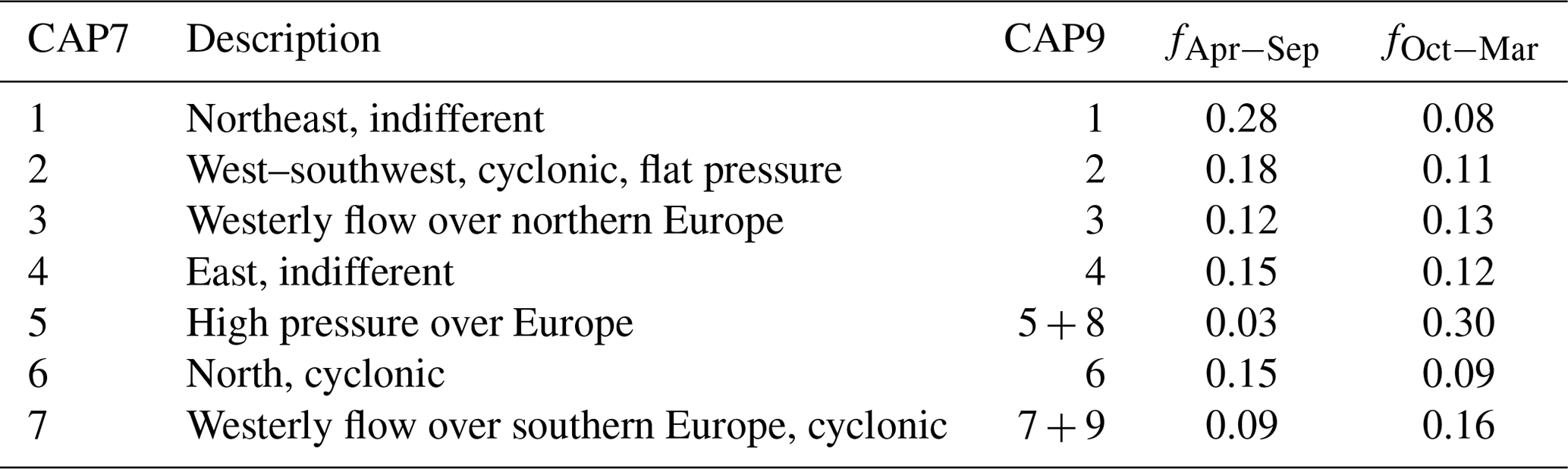
In addition to the reconstructed fields, I also use Swiss weather types, which are available for every day back to 1763 (Schwander et al., 2017). For each day, the data set provides the most likely of seven weather types, along with its probability. Each weather type can be equated to a short meteorological description of the weather. The seven weather types (termed CAP7, where CAP stands for cluster analysis of principal components) are based on the so-called CAP9 weather types of MeteoSwiss (Weusthoff, 2011), which encompass nine types. The reduction to seven types (by combining existing types) was necessary as in the early decades, some types could not be well discriminated; Table 1 shows an overview.

Table 1 Description of CAP7 weather types, corresponding CAP9 types, and frequencies in the cold and warm season in the period 1961–1990.

2.2 Data for comparison: man-made documentary evidence

The gridded reconstruction is based only on instrumental measurements from three stations. In a recent project we have uncovered (Pfister et al., 2019) and digitised (Brugnara et al., 2020) many more instrumental series for Switzerland back to the early 18th century, such that we now have 10 series for 1816. This effort was part of a global effort to uncover more historical instrumental data (Brönnimann et al., 2019b), a lot of which is currently being digitised. With these data, more accurate reconstructions will be produced in the future. The Swiss data could be used to independently evaluate the reconstruction used here, but I touch on this only briefly as it is not the goal of this paper. Rather, most of these additional series also have categorised daily weather observations, and some have descriptive monthly summaries. In this paper I focus on these entries for three series: Geneva, Aarau, and St. Gall. These three series are described in the following; they can be downloaded from EURO-CLIMHIST (Pfister et al., 2017).

The Aarau weather data, published in the journal Archiv der Medizin, Chirurgie und Pharmazie (Zschokke, 1817) contain twice or three times daily instrumental measurements (pressure, temperature) and non-instrumental observations (whether or not there was precipitation; sky cover) (Faden et al., 2020). An example for September 1816 is given in Fig. 1. The weather data were recorded by Heinrich Zschokke (1771–1848), a German-born teacher and politician. The record was continued by his son and overall covers almost 60 years.

Figure 1 Weather observations by Zschokke, Aarau, for July 1816 (Zschokke, 1817).

Likewise, the St. Gall record contains instrumental (temperature, pressure) and non-instrumental (precipitation, sky cover) information, recorded twice daily. The observations were made by pharmacist Daniel Meyer (1778–1864) from 1812 to 1832 and continued by other, unknown observers (Hürzeler et al., 2020). The data were published in the journal Der Erzähler (Meyer, 1816, 1817).

The series from Geneva (Auchmann et al., 2012) was observed by Marc-Auguste Pictet (1752–1825), a scientist and publisher from Geneva. He was director of the Geneva Observatory; in fact, he may rightly be called a meteorologist. His observations, published monthly in the journal Bibliothèque universelle (Pictet, 1816), also include monthly summaries with notes on the state of vegetation. Note that the instrumental measurements from Geneva were used to produce the daily numerical reconstruction, so they are not independent. Therefore, I do not compare the daily entries here but rather the monthly summaries.

Finally, I also briefly use weather observations made by a person named Furrer in Winterthur from 1849 to 1867 (Pfister et al., 2019). The data were taken from the Zurich State Archive. They are used to test my approach in a later period, when better reconstructions are available.

2.3 Data for comparison: weather diary

Synthetic weather diaries can also be generated for journeys. To test this, I used the travel diary of Lord Byron during his famous voyage from Lake Geneva through the Bernese Oberland in September 1816. I extracted several weather-related statements from his travel journal (Byron, 1839) and extracted the same information, in space and time, from the numerical reconstruction.

3 Method

3.1 General concept and reference period

In order to make the weather reconstructions as useful as possible to non-climatologists, while allowing us to better compare them to weather observation notes, I structured the data in a similar way as found in many observation books. Daily values and descriptors are listed, and for each month a summary is given.

• -

  For each day, the absolute number is given for T_mean and precipitation, accompanied by additional information (relating to a reference period, see below) and a set of descriptive qualifiers concerning each variable and the weather type.

• -

  For each month, monthly statistics are given for T_mean and precipitation in numerical form. Additionally, monthly indices are calculated and given numerically. Again, this section is accompanied by descriptive qualifiers for both the monthly weather and the indices.

Observers might sometimes report on temperature in an “absolute” manner (e.g. referring to freezing), but often also in a relative way (e.g. “very cold day”) based on their own experience and perhaps in some cases alluding to societal memory. This requires information on the observers and observation context. For this study this implies putting absolute numbers in the context of a reference period. For consistency, I use the same reference period as in Flückiger et al. (2017): the period 1800–1820 without the volcanically perturbed years 1809–1911 and 1815–1817. Fields of reference period mean temperature for every calendar day are available from Flückiger et al. (2017), so results presented here can be compared with that study. However, obviously a historical observer would not have a memory of the future.

Note that Flückiger et al. (2017) did not reconstruct every day in the historical reference period. Rather, they defined a present-day reference period (1982–2009) from which they subtracted the difference (in terms of a seasonal cycle) between the periods 1800–1820 and 1982–2009 based on instrumental observations from the three mentioned stations for the historical reference period. For precipitation and solar irradiance, no change was added and thus 1982–2009 is considered as a reference period for these two variables. In this paper, for consistency, I follow the same approach.

Historical observers, in their reporting, might account for the changing variability in the course of the seasons. For instance, variability is larger in winter than in summer. Temperature on a cold summer day might be less below average (in degrees Celsius) than on a cold winter day. I therefore standardised the anomalies, again using the 1982–2009 standard deviation (calculated for each calendar day and then smoothed by fitting the first two harmonics of the seasonal cycle). Likewise, monthly averages or monthly statistics were expressed as standardised anomalies by using the reference period annual cycle and standard deviations calculated per calendar month.

3.2 Obtaining daily weather descriptions

The first step to obtain daily weather descriptions is to establish a taxonomy that eventually allows a comparison between observations and numerical reconstructions. The target taxonomy must be reducible to the observed taxonomy but ideally contains additional information. The observations by both Zschokke and Meyer were already extremely standardised. With respect to precipitation, the main categories are rain, snow, or an empty field (standing for dry). In the case of Zschokke, we also (rarely) find the terms “Schneeregen” (mix of snow and rain) and “Staubregen” (most likely: drizzle).¹ In the case of Winterthur, which was used for testing the method in 1864–1866, we also find “Nebelregen”, “Nebel”, and “neblig” (fog rain, fog, foggy; for the comparison we assume that precipitation amounts are below the detection threshold chosen in the next section.).

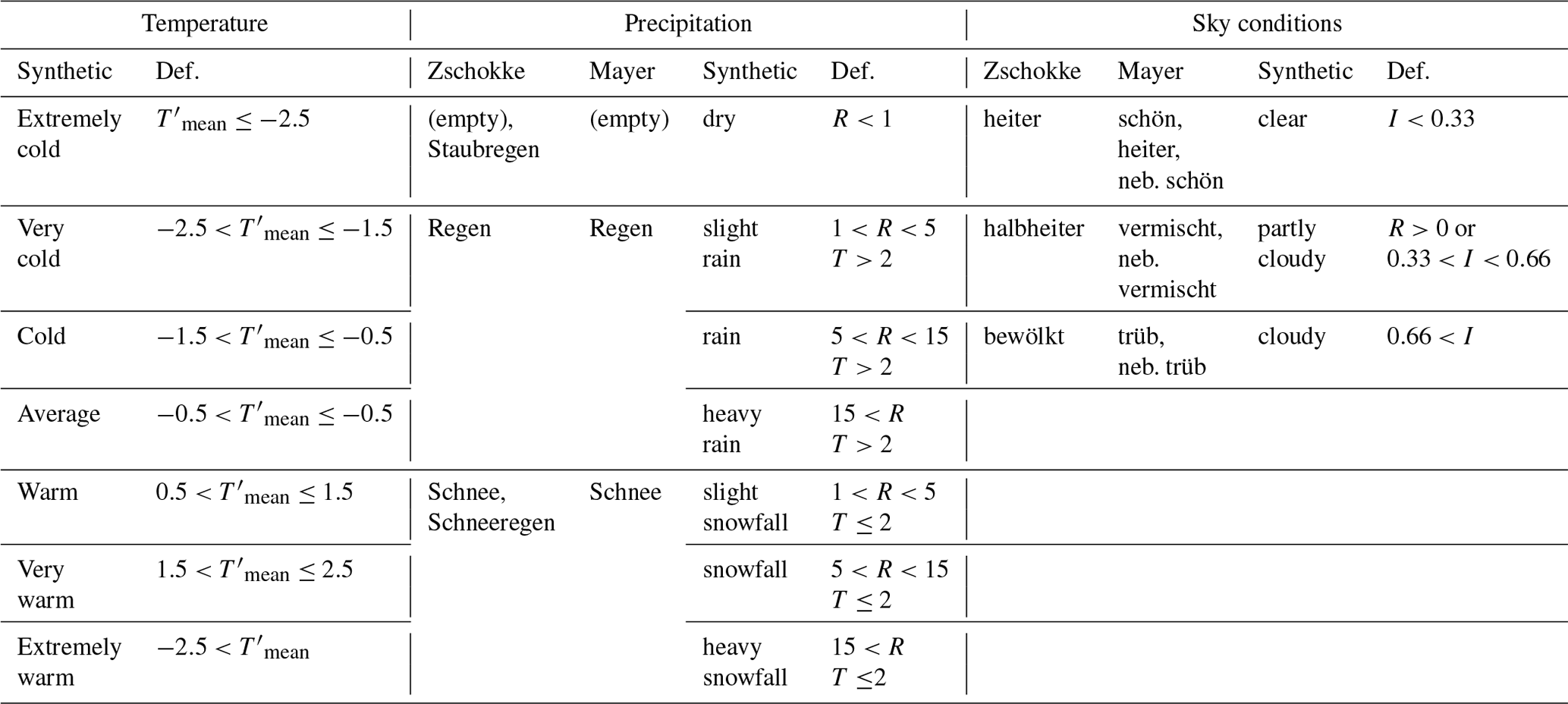
In short, Zschokke and Mayer both provide basically three categories (rain, snow, or dry), two or three times per day. The synthetic weather diary only has daily resolution (so the observations need to be aggregated for comparison), but information can be categorised into more classes which can then be aggregated. The definitions of the classes are indicated in Table 2 and described in more detail in the following.

Table 2 Taxonomy used in the observations from Zschokke and Mayer as well as in the synthetic weather diary, together with the definition (def.; T: daily mean temperature in ^∘C; T^′: standardised daily mean temperature anomaly; R: precipitation in millimetre per day; I: irradiance relative to possible irradiance).

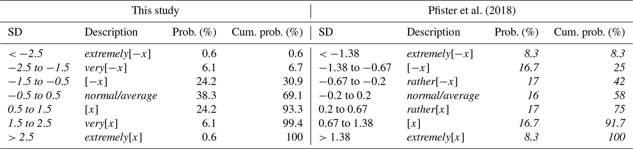
For all standardised anomalies (daily or monthly) we use a seven-point scale defined in Table 3. Note that this scale deviates from similar seven-point scales as defined, e.g. by Pfister et al. (2018), which is also included in Table 3. This is because on the daily scale, a non-linear (in terms of the underlying variable; the scale is almost linear in terms of probabilities) categorisation as implied by the Pfister indices seems hard to achieve; it would require detecting rather subtle changes close to the average. Therefore a linear scale is preferred. The basic categories −x or x (e.g. cold or “warm”) are similar in the two classifications, with thresholds roughly near the quartiles, but there is a large discrepancy in the use of the term “extreme”. There is approximate agreement of my scale with the likelihood scale in the IPCC calibrated language (IPCC, 2013) where “likely” and “very likely” refer to 66 % and 90 % cumulative probability (in my scale “x” and “very x” refer to 69.1 % and 93.3 %, respectively). However, the scale can easily be adapted, and indeed should be adapted, for other applications.

Table 3 Seven-point scale for indexing standardised anomalies (SD), description (x denotes a property and −x its reverse, e.g. “warm” and “cold”, “wet” and “dry”, or “late” and “early”) and corresponding probabilities (prob.) and cumulative probabilities (cum. prob.) for (left part of table) this study and (right) (Pfister et al., 2018). Italics: thresholds and descriptions that are part of the definition; other columns are implied by assuming a normal distribution.

For the daily values, the following information is given.

• -

  For T_mean the synthetic weather diary contains the absolute values, the anomaly from a contemporary reference period, and the standardised anomaly. The taxonomy is based on the latter, using the seven-point scale (Table 3): values $<-\mathrm{2.5}$ are termed “extremely cold”, −2.5 to −1.5 “very cold”, −1.5 to −0.5 “cold”, −0.5 to 0.5 “average”, 0.5 to 1.5 “warm”, 1.5 to 2.5 “very warm”, and >2.5 “extremely warm”.

• -

  For precipitation the synthetic diary gives the absolute value as well as the qualifier “dry” (<1 mm), “slight rain” (1 to 5 mm), “rain” (5 to 15 mm), and “heavy rain” (>15 mm). The thresholds are chosen arbitrarily. For the case of Geneva, 69 % of the days in the reference period are “dry”. Of the remaining days, half have “slight rain”, 36 % have “rain”, and 14 % “heavy rain”. The sensitivity to the choice of the thresholds is analysed later. If daily mean temperature was below 2 ^∘C (following Zubler et al., 2014), the qualifiers “slight snowfall”, “snowfall”, “heavy snowfall” are used instead.

• -

  Sky conditions are given as text. For this, irradiance was first expressed as fraction of the maximum possible value for the corresponding calendar day. The latter was approximated here by the simple function $\mathrm{100}\times (\mathrm{1.4}\mathrm{W}{\mathrm{m}}^{-\mathrm{2}}-\cos (w\left)\right)$, where w is the angle corresponding to the calendar day centred around the solstices. If the fraction is higher than 0.66 and no precipitation is reconstructed, the sky is described as “clear”; if it is below 0.66, or if there is precipitation, it is described as“partly cloudy”, and if it is below 0.33, it is described as “cloudy”.

• -

  Finally, I provide the most likely weather type for that day from the Swiss CAP7 weather statistics (Schwander et al., 2017), along with the probability of that weather type on that day and a text description of the type. Note that the weather type cannot directly be compared with the (often observed) wind direction unless the local situation is very well understood. However, for future applications, wind would be an important component of a synthetic weather diary.

Note that irradiance was calculated from an interpolation of few station data and should only be analysed close to current weather stations, which is the case for the four extracted weather diaries. However, spatial field cannot be analysed, and I do not provide numerical values in the synthetic weather diaries.

3.3 Monthly weather summaries

For each month, the following information is given:

• -

  mean T_mean of the month, again along with the deviation from the reference and a qualifier (seven-point scale, Table 3), and the number of freezing days (T_mean<0 ^∘C),

• -

  precipitation sum (also expressed as percentage of the reference for that calendar month) and number of rain or snow days,

• -

  monthly counts of the seven weather types (also expressed as percentage of the corresponding relative frequency for that calendar month in the reference period), and

• -

  three derived indices described below: growing degree days, maximum 10 d value of freezing degree days, and water balance, each given as absolute value and qualifiers.

This information can further be condensed, if necessary. The following monthly indices are used.

• -

  Growing degree days (GDDs): the cumulative sum of T_mean above 4 ^∘C (starting on 1 January) is a measure for suitability for crop growth. Each month I give the value for that month (with reference) as well as the delay at the end of the month with respect to the median in the reference period and a qualitative description (“extremely early” to “extremely late”, according to standardised anomalies using the seven-point scale). While leaf unfolding or flowering quite generally depends on GDD, crop maturity (and thus harvest dates) or leaf colouring are more species dependent and depend on other factors. Therefore, GDD delays and qualifiers are only given for the months of March to July.

• -

  Freezing degree days (FDDs): the cumulative sum of T_mean below 0 ^∘C (with a positive sign), accumulated over the 10 previous days. For the months January to April and October to December, the maximum of this 10 d index per month (max₁₀FDD) is given. If maximum FDD exceeds 50 ^∘C, then a note “small lakes frozen” is indicated; if it exceeds 90 ^∘C, “large lakes frozen” is indicated (note that in the example given in this paper, neither case occurs). These thresholds are in approximate agreement with Franssen and Scherrer (2008) but, again, would have to be adapted for each application.

• -

  A monthly index of the water balance (precipitation minus potential evapotranspiration, P−E) is calculated by making use of the precipitation amount and T_mean, from which potential evapotranspiration is calculated using the Thornthwaite (1948) formula. The monthly balance is standardised and then described in each month with the seven-point scale (“extremely wet” to “extremely dry”).

4 Results

4.1 Man-made documentary evidence for Aarau and St. Gall

The synthetic weather diaries for Aarau and St. Gall are given in the Supplement. Their performance in terms of temperature can be measured by comparing the numerical values with the instrumental temperature series from the two stations, which were not used in the reconstruction process and are thus independent. After subtracting the mean annual cycle in the reference period from both series (by fitting the first two harmonics of the seasonal cycle), I find a correlation of 0.81 and 0.72. Note that the measurements themselves have errors. In view of that, the correlations indicate that even though the reconstruction is based on only three stations, the temperature fields are quite reliable.

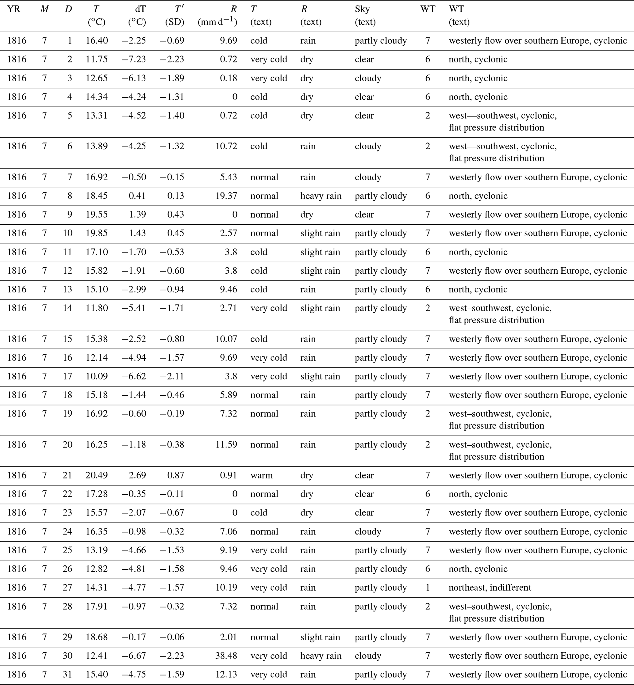
For rainfall and sky cover, I compare our synthetic diaries with the actual observations from the two stations. As an example, the Aarau observations for July 1816 are shown in Fig. 1, the corresponding synthetic diary in Table 4. Both the observations and the synthetic diary indicate a particularly rainy month, but on a day-to-day scale there are also clear differences. In the observation, there are only 3 d without any precipitation (20, 21, and 23 July), of which two are also dry in the synthetic diary. The latter gives 8 “dry” days (of which 4 have zero precipitation and 4 have less than 1 mm).

Table 4 Synthetic weather diary for Aarau, July 1816 (columns: YR: year; M: month; D: day; T: daily mean temperature; dT: daily mean temperature anomaly; T^′: standardised daily mean temperature anomaly; R: precipitation; the subsequent columns give text descriptions of temperature, precipitation, sky conditions, and weather type respectively).

A plot comparing observations and synthetic weather diary for both stations for both precipitation and sky conditions is shown in Fig. 2b–e. While the agreement at the level of seasonal characteristics is quite favourable – both synthetic weather diaries and observations confirm the high number of rainy days in summer and also agree on less rainy periods – there are also important differences. For instance, the first half of September is rather dry in the synthetic diaries (both Aarau and St. Gall), but many rainy days are reported at both stations.

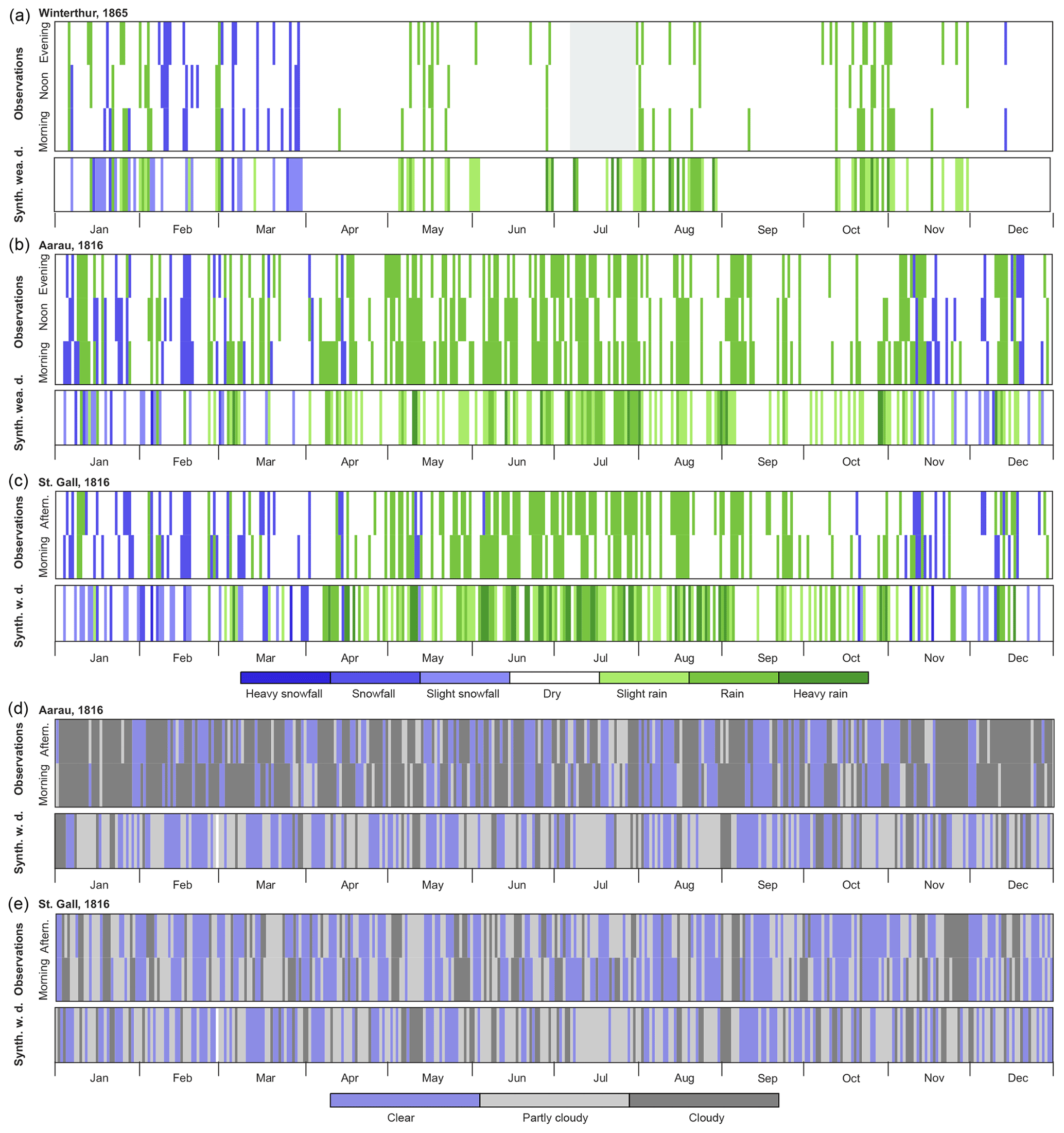
Figure 2 Comparison of observations (two–three times daily) and synthetic weather diaries (daily) for Winterthur (1865) (a) as well as Aarau (b) and St. Gall (c) (1816) for precipitation and for Aarau (d) and St. Gall (e) for sky cover. Grey shading in (a) indicates an observation gap.

The agreement can be quantified with Spearman correlations by coding rain/no rain in the observations as 0 and 1 (“Nebelregen”, “Nebel”, “neblig”, and “Staubregen” were set to 0) and in the synthetic diary as 0 to 3 for “dry”, “slight rain/snowfall”, “rain/snowfall”, and “heavy rain/snowfall”. In this way I find correlations of around 0.25 for Aarau and St. Gall. When coding snow with a negative sign in both sources, correlations increase to slightly above 0.4 at both sites. Although highly significant, this agreement may not be good enough yet to be useful on a day-to-day scale.

There are several causes for discrepancies: errors in the reconstruction, errors in the observations, lack of representativity of observations for a grid cell, and inadequate translation. The error in the reconstructions can be partly assessed by comparison with similar analyses in a period after 1864, when better reconstructions are available (Pfister et al., 2020). In these reconstructions, the error in precipitation was assessed by subsampling in the 1961–2010 period. Correlations of 0.75–0.90 were found for most parts of Switzerland, which, however, constitutes an upper-limit estimate as this analysis has no representativity error and a good quality of the underlying measurements. A more realistic case is to analyse these reconstructions in the very early years of the Swiss Meteorological network. Non-instrumental observations are available, for instance, for Winterthur. Comparing rainfall in the first 3 years (1864–1866) in the same way (coding snow with a negative sign), I find a correlation of 0.5. This analysis accounts for the same errors as in the case of 1816, the only difference being better reconstructions. This estimate is an upper limit of the quality that can possibly be reached 250 years back using additionally digitised data (Brugnara et al., 2020). For the year 1865, the comparison is also shown in Fig. 2a. Clearly the agreement is better in this case (note also the period of missing observations in July, for which the synthetic diary indicates several rainy days). Most importantly, the difference between this relatively dry year and the wet year 1816 is extremely clear. In Fig. S1 in the Supplement I also show the years 1864 and 1866, which were closer to average in terms of precipitation. The agreement is similar to that for 1865, except perhaps for the summer of 1866, which is slightly worse.

The error in the translation could be assessed by changing the thresholds chosen. In the case of Aarau, the threshold for precipitation could have been set too high in the synthetic diary. I tested all combinations of threshold of 0.5 or 1 mm, 5 or 8 mm, and 15 or 20 mm for the separation between the four classes for both Aarau and St. Gall. In fact, most other combinations gave slightly better results (e.g. 0.5, 8, 20 mm), but differences were small. In any case, for other applications the thresholds would have to be reconsidered.

Finally, the agreement between observed and synthetic sky conditions is very low. Correlations, defined similarly as above, yield coefficients of 0.06 and 0.12 for St. Gall and Aarau, respectively, which is too low to be useful. Visually, large differences become apparent between the observations at Aarau and St. Gall. Specifically, the category “cloudy” (“bewölkt” in Zschokke, “trüb” or “neb. trüb” in Mayer) differs a lot between the sites at the expense of “partly cloudy”. More work and more care is required to obtain a good classification.

The weather type information can give additional information. For instance, every day but one (27 July) in the example of July 1816 is attributed to a cyclonic weather type. This agrees well with the rainy character of the month. Note also the frequent westerly winds noted in the observations, which are in accordance with westerly or west–southwesterly weather types, although in that case knowledge of the local wind situation and the channelling of winds is required.

4.2 Monthly summaries for Geneva

For testing the monthly summaries in the synthetic weather diaries, I compare them with the observations from Geneva. Marc-Auguste Pictet, in his observations published in the Bibliothèque universelle also gives a monthly summary. This sort of information is typical in historical weather sources. Here I compare the entries for the months of March to September, which are most relevant for crops, in a qualitative way (Table 5). Note that for this table, for brevity's sake, the synthetic monthly summaries have been further simplified (e.g. not all weather types are indicated but only those that were anomalously frequent or infrequent).

Table 5 Comparison of monthly summaries of weather and state of vegetation by Pictet (1816) in Geneva (my translation) and in our synthetic weather diary (excerpt giving monthly mean temperature, number of frost days (if any), max₁₀FDD, GDD, delay, monthly mean rainfall, percentage of normal rainfall, number of rain and snowfall days, P−E with qualifier, overview of frequent (>150 %) and infrequent (<50 % relative to expected frequency from reference period) weather types, with number and percentage compared to reference period). Highlighted in italics are text excerpts (left) that can qualitatively be compared with the synthetic diary (right).

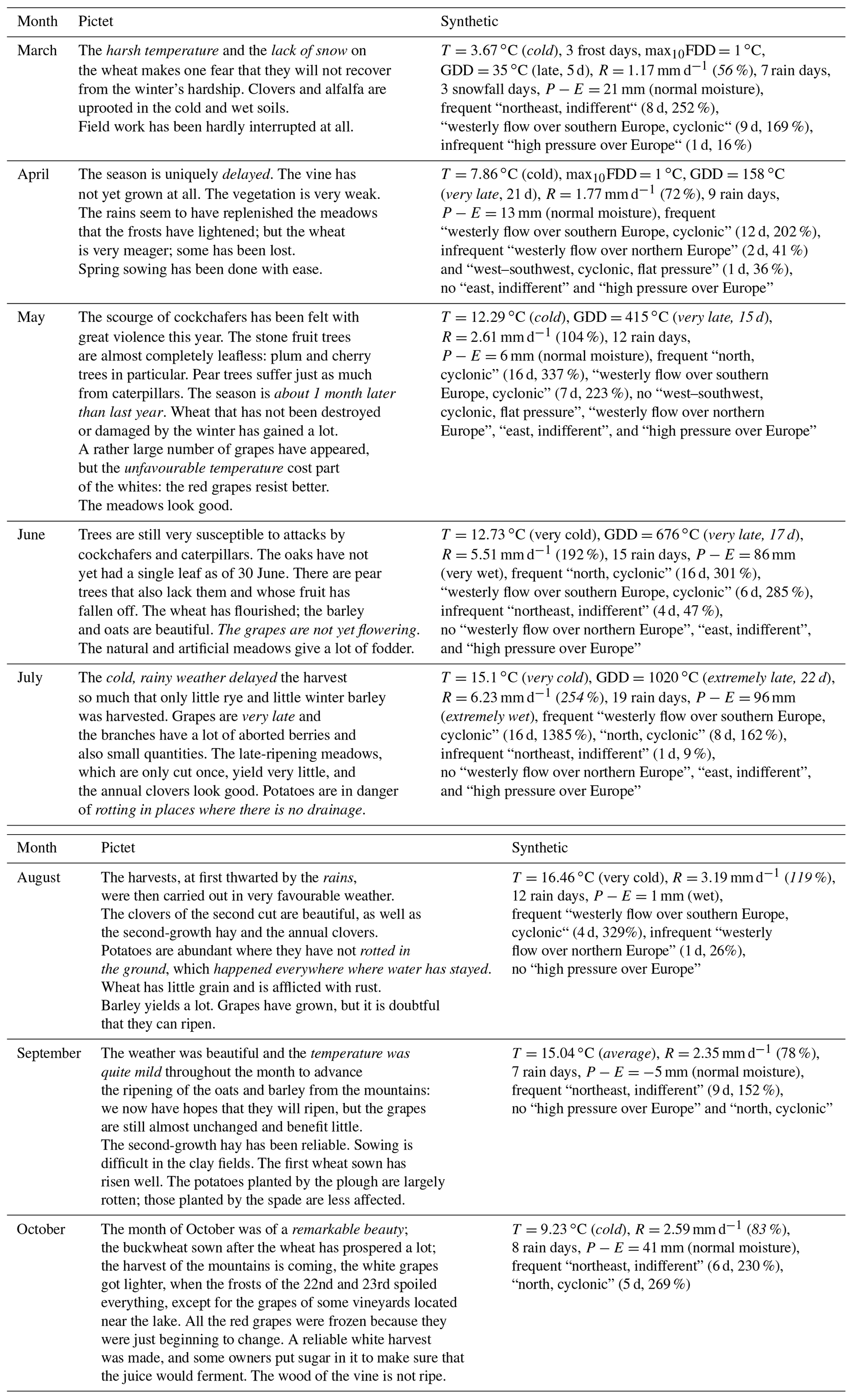
The comparison (highlighted in italics) shows a relatively good agreement. Almost in all months, Pictet points to the delay of vegetation, which is also seen in the synthetic diary based on growing degree days. The calculated delay reaches 22 d in July (relative to the historical reference period). This is less than indicated by Pictet (1 month), which, however, refers to one comparison year. Agreement is also found with respect to most mentions of temperature and rainfall. For instance, the reported “harsh temperatures” in March correspond to a cold month in the synthetic diary, the “cold and rainy weather” in July compares well with the characterisation “very cold” and “extremely wet” in the synthetic diary. Worse agreement is found for October, which according to Pictet was of “remarkable beauty” but in the synthetic weather diary is characterised as “cold”, though with below normal rainfall.

4.3 Comparison with Lord Byron's journey

A possible example of the use of synthetic weather diary is to track the weather experienced during an expedition or journey. As an example, I use the famous journey of Lord Byron through the Swiss Alps in September 1816. After a dreadful summer with almost constant rain, the weather was improving and Lord Byron found the weather to be quite nice during the trip.

Figure 3 shows the reconstructed fields for 5 d in September 1816, along with a dot that marks the location of Byron as well as the weather descriptions from his diary and from the synthetic weather diary, calculated for each location. The first day (“fine weather”) indeed was a nice day also in the reconstructions, with no rainfall and high temperatures. Agreement is also found on the other days, both in terms of rainfall and temperature, except perhaps for 25 September, when Byron notes “the weather has been tolerable all day” (the meaning of which, however, is unclear). On this day, the reconstruction shows spatially extensive (though not extremely intense) rainfall. The two stations Aarau and St. Gall also report rainfall.

Figure 3 The weather during Lord Byron's travel from Lake Geneva to the Bernese Oberland in September 1816. The figure shows his diary entries (in quotation marks) as well as the synthetic weather diary for 5 d. Also shown are precipitation and daily mean temperature from the reconstructions. The green dot marks the position of Lord Byron. The small dots indicate whether the observers at Aarau and St. Gall noted precipitation (blue) or not (grey).

5 Discussion

The analyses show that synthetic diaries can provide local, daily weather information in a format that is comparable to non-instrumental observations and weather descriptions in diaries. The comparison with independent observations shows some agreement, although the quality both of the daily reconstruction as well as of the translation needs further improvement.

The comparison of monthly summaries also showed a good agreement and points to the usefulness of vegetation indices (such as GDD). The monthly summary also points to the effect of combinations of factors (e.g. cold with little snow) and the importance of pests and insects for agriculture. Experts might be able to make use of the numerical reconstructions or the synthetic weather data also for analysing insect infestations. In his summaries, Pictet appears as a rather reserved observer, who largely excludes the societal effects in his descriptions. Other weather diaries from this time (e.g. the Hoffmann diary, quoted in Bodenmann et al., 2011) have a more pessimistic or even desperate tone, list in detail the prices, and point to the miserable situation, to beggars etc.

The comparison with the travel diary of Lord Byron yields a general agreement. This shows that synthetic weather diaries might be useful as an additional information source to better analyse the journey.

For all analyses, we should note that rainfall is much more difficult to reconstruct by the analogue method than temperature due to its very high spatial variability (Pfister et al., 2020). Moreover, there is a large representativity error and arguably also a large observation error. For instance, rain may fall unnoticed during the night. Moreover, instrumental precipitation (which is the basis for the analogue method) is defined as 6:00 UTC to 6:00 UTC the next day, making comparison at times more difficult; a one-day shift is possible. Note also that the 2×2 km² grid does not represent the resolution of the observing network, which has a typical inter-station difference of 15–20 km (MeteoSwiss, 2019). In any case, precipitation can only be taken as a rough indication. Temperature, conversely, is well reconstructed but less often in the focus of observers. Eventually, wind would be an important variable for any reconstruction, which should be considered in future approaches.

While the agreement as measured in correlation is at times low, currently limiting the application of synthetic diaries, it should be noted that future reconstructions will likely be much improved and resolve further detail. Daily weather reconstructions could also be produced for other regions in Europe with the analogue approach, provided that high-resolution data sets are available for a recent period as a pool of analogues (for Europe, E-OBS provides daily fields back to 1950 at 0.1^∘ resolution; Haylock et al., 2008). Daily high-resolution weather reconstructions could also be produced from dynamical downscaling of reanalyses (Slivinski et al., 2019). Once such high-resolution daily weather reconstructions are available, the potential is immense. Weather information can be generated for military operations or other weather-sensitive activities. Synthetic weather diaries can also be produced for travels and expeditions. The translation into text as well as the comparison with reference periods allows a more direct comparison, and the calculated indices may be useful for some applications. In particular, impacts on agriculture or on other areas of life can be assessed more easily. In short, synthetic weather diaries could be used in a variety of ways by historians to constrain, cross-date, compare, or complement other information.

The approach is however also important for science. If the translation from numeric weather data to a synthetic diary that resembles historical sources succeeds, inversion methods can be used to do the opposite: reconstruct weather numerically from descriptive data. Data assimilation techniques use such “forward models”; however, for a formal data assimilation approach the variables need to be on a metric scale. For other approaches, such as analogue selections, the variables must at least allow the expression of similarities (or ordinal distances). Systematically compiled categorial information, however, as is produced in our approach, could be used for instance by machine learning approaches. This requires that historical weather diaries can be categorised (or are already categorised) in a prior step. If this is the case, machine learning approaches could then be trained on synthetic weather diaries generated in the most recent few decades to provide weather types, or even entire weather fields. Once successfully trained, such approaches can then applied to past weather diaries.

6 Summary and conclusions

Recent efforts in climatology have resulted in daily weather reconstructions for the globe covering the last 200 years. Daily weather reconstructions are also generated for specific regions at high resolution and might soon reach 250 years back. These data sets could be important for history and science. In this paper I explore this by translating a high-resolution, prototype weather reconstruction for Switzerland, 1816, into synthetic weather diaries for selected locations. These synthetic weather diaries not only provide the reconstructed values but translate them into a categorial form that makes them comparable to weather descriptions. Reconstructed values are referenced to a contemporary reference period, and a calibrated language (e.g. “very cold”) is used to translate numbers to categories. Furthermore, monthly summaries are provided, using the monthly statistics of the daily reconstruction (translated to descriptive categories) as well as indices for plant growth, freezing, and drought (also translated to descriptive categories).

Results from our prototype reconstructions for Switzerland, 1816, show good agreement with independent early-instrumental measurements and non-instrumental daily weather observations from Aarau and St. Gall and with monthly weather summaries from Geneva. Also, qualitative agreement with the travel diary of Lord Byron on his journey through Switzerland in September 1816 is found. The quality of this pilot reconstruction is arguably not accurate enough for many applications. However, future products are expected to be of sufficient quality to yield useful information, although there will always be substantial uncertainty for rainfall and particularly for sky conditions.

Synthetic weather diaries are also relevant for science. Combined with machine learning approaches, they could be used to reconstruct weather numerically from descriptive data. This opens an immense potential for the use of existing databases of historical weather data such as EURO-CLIMHIST (Pfister et al., 2017), Tambora.org (Riemann et al., 2015), and TEMPEST (Veale et al., 2017) but requires intense collaboration between historians and scientists.