Comparison of observed borehole temperatures in Antarctica with simulations using a forward model driven by climate model outputs covering the past millennium

The reconstructed surface-temperature time series from boreholes in Antarctica have significantly contributed to our understanding of multidecadal and centennial temperature changes and thus provide a good way to evaluate the ability of climate models to reproduce low-frequency climate variability. However, up to now, there has not been any systematic model–data comparison based on temperature from boreholes at a regional or local scale in Antarctica. Here, we discuss two different ways to perform such a comparison using borehole measurements and the corresponding reconstructions of surface temperature at the West Antarctic Ice Sheet (WAIS) Divide, Larissa, Mill Island, and Styx Glacier in Antarctica. The standard approach is to compare the surface temperature simulated by the climate model at the grid cell closest to each site with the reconstructions in the time domain derived from the borehole temperature observations. Although some characteristics of the reconstructions, for instance the nonuniform smoothing, limit to some extent the model–data comparison, several robust features can be evaluated. In addition, a more direct model–data comparison based on the temperature measured in the boreholes is conducted using a forward model that simulates explicitly the subsurface temperature profiles when driven with climate model outputs. This comparison in the depth domain is not only generally consistent with observations made in the time domain but also provides information that cannot easily be inferred from the comparison in the time domain. The major results from these comparisons are used to derive metrics that can be applied for future model–data comparison. We also describe the spatial representativity of the sites chosen for the metrics. The long-term cooling trend in West Antarctica from 1000 to 1600 CE (−1.0 ^∘C) is generally reproduced by the models but often with a weaker amplitude. The 19th century cooling in the Antarctic Peninsula (−0.94 ^∘C) is not reproduced by any of the models, which tend to show warming instead. The trend over the last 50 years is generally well reproduced in West Antarctica and at Larissa (Antarctic Peninsula) but overestimated at other sites. The wide range of simulated trends indicates the importance of internal variability in the observed trends and shows the value of model–data comparison to investigate the response to forcings.

1 Introduction

Although most of the world has been steadily warming over the last few decades, the temperature trend in Antarctica is not homogeneous (Jones et al., 2016). Several syntheses relying on instrumental air temperature records have shown a large recent warming over the Antarctic Peninsula (AP) and parts of West Antarctica, but the trend for the other parts of the Antarctic continent remains less clear (Chapman and Walsh, 2007; Nicolas and Bromwich, 2014; Steig et al., 2009; Turner et al., 2005). It remains difficult to characterize the large interannual to multidecadal variability at high southern latitudes because instrumental data are sparse and limited to the last 60 years, at best. The mechanisms at the origin of recent changes are thus still uncertain (Goosse et al., 2012; Jones et al., 2016; Nicolas and Bromwich, 2014).

Proxy-based reconstructions offer the opportunity to place the recent temperature changes in a longer context. Thanks to their relatively good spatial coverage and high resolution, the reconstructions based on water-stable isotopes derived from ice cores have provided important information on temperature variability during the past two millennia over Antarctica. They indicate a significant cooling trend during the preindustrial period across all Antarctic regions and confirm the strong spatial heterogeneity of the recent warming (Goosse, 2012; Schneider et al., 2006; Stenni et al., 2017). However, the link between the isotope records and local climate is complicated, and this introduces significant uncertainties in the reconstructions (Stenni et al., 2017; Klein et al., 2019).

Borehole temperature observations provide another opportunity to reconstruct surface temperature, and several studies have demonstrated their interest, particularly over Antarctica (i.e., Barrett et al., 2009; Muto et al., 2011; Orsi et al., 2012; Zagorodnov et al., 2012; Roberts et al., 2013; Yang et al., 2018). The most significant advantage of borehole paleothermometry is that temperature is directly measured with a thermistor calibrated in the laboratory. Therefore, the calibration is independent of the climate at the measurement site. Nevertheless, the characteristics of heat conduction that blur the surface temperature history make the reconstruction mathematically underdetermined: several temperature histories can result in the same borehole temperature profile, because diffusion will smooth out high-frequency temperature variations. Consequently, the temperature history cannot be determined unequivocally. Several approaches have been proposed to overcome the problem, as synthesized in Orsi et al. (2012), for instance the Bayesian reversible jump Markov chain Monte Carlo (Dahl-Jensen et al., 1999) and the generalized least-squares inversion (Muto et al., 2011; Orsi et al., 2012; Yang et al., 2018). By applying these methods, the reconstructed temperature series have presented evidence of the existence of cold conditions corresponding to the Little Ice Age in West Antarctica from 1300 to 1800 CE (Orsi et al., 2012), as well as of a recent warming trend in West Antarctica (Barrett et al., 2009; Orsi et al., 2012; Yang et al., 2018), at some high-elevation sites of the East Antarctica (Muto et al., 2011; Roberts et al., 2013) and over the AP (Zagorodnov et al., 2012), though the timing and magnitude vary between regions.

The reconstructed temperatures based on isotopic composition have been compared to results of climate models. Most models display a relatively large and homogenous warming over Antarctica since 1850 CE, which is inconsistent with the signal inferred from the isotope records (Goosse et al., 2012; Klein et al., 2019; Stenni et al., 2017; Abram et al., 2016). This disagreement may be due to the uncertainties in the reconstructions or due to the biases in the climate models that may overestimate the response to greenhouse gas forcing or underestimate the natural climate variability in the region (Jones et al., 2016; Neukom et al., 2014). However, a recent study assessing the link between isotope record from ice cores and regional climate over Antarctica using pseudoproxy and data assimilation experiments has not been able to identify any systematic bias in reconstructions on continental-scale temperatures based on δ¹⁸O (Klein et al., 2019).

Up to now, there were no systematic model–data comparisons for temperature reconstructed from boreholes at a regional or local scale in Antarctica. This is, in part, due to the characteristics of the inversion that imposes smoothing on a time window that increases as we go back in time and makes the comparison with the simulated surface temperature difficult (Beltrami et al., 2006; Harris and Gosnold, 1999). Additionally, some reconstructions have an uncertainty range of the same magnitude as the full variability provided by the climate model results, which seriously limits the interest of model–data comparison.

As some of the difficulties in the comparison between the simulated surface temperature from climate model results and the reconstructions from boreholes come from the inversion procedure, comparing directly the observed profile with the one obtained using a one-dimensional heat advection and diffusion forward model can provide new insight. This approach is an example of the application of proxy system models (PSMs) that reproduce directly processes responsible for the signal recorded in the archive (Evans et al., 2013). PSMs have been applied recently for several proxies, such as tree ring width or water isotopes in ice cores, corals, tree ring cellulose, and speleothem calcite (Evans et al., 2013; Dee et al., 2015). The application of climate model outputs to drive a borehole temperature forward model has demonstrated the strong coupling between near-surface air and ground temperature changes over decades to centuries (e.g., Beltrami et al., 2005; García-García et al., 2016; González-Rouco et al., 2003, 2006) and has also been used to validate climate model outputs (e.g., Beltrami et al., 2006; Stevens et al., 2008).

Nevertheless, using a PSM introduces some uncertainties that must be taken into account. A critical point for borehole temperature is the potential influence of long-term climate changes, such as glacial to interglacial cycles, which is difficult to estimate (Orsi et al., 2012; Rath et al., 2012). In addition, the simulated subsurface temperature profiles in Antarctica are sensitive to model parameters and inputs, such as snow accumulation, ice thickness, geothermal heat flow, and the physical properties of ice or ground, which may have significant uncertainties.

Previous studies using forward models driven by climate model outputs were focused on ground temperature (e.g., Beltrami et al., 2005; García-García et al., 2016; González-Rouco et al., 2003, 2006) and not on boreholes obtained in the ice. Here, we will fill this gap by simulating directly subsurface temperature for the publicly available borehole profiles covering the past centuries in Antarctica, using the one-dimensional heat advection and diffusion forward model of Orsi et al. (2012). Our goal is to provide a protocol for evaluating the climate model ability to reproduce observed low-frequency (multidecadal- to centennial-scale) variability. We will analyze two model–data comparison methods to identify the potential advantages and drawbacks of each approach. The easiest way is to directly compare the surface temperature reconstructed from the borehole measurements with the surface-temperature time series simulated by the climate model at the grid cell closest to each site. The second way is to compare the simulated subsurface borehole temperature with the observation by driving the forward model with climate model outputs. In this case, we analyze the temperature at a fixed time as a function of depth. For simplicity, we will later refer to those two methods as a comparison in the time domain and depth domain, respectively.

This study is organized as follows. The borehole temperature observations, climate model results, forward model, and sensitivity of the results to key parameters of the forward model are briefly described in Sect. 2. Section 3 presents the comparison of simulated and reconstructed surface air temperatures and the comparisons of simulated and observed borehole temperature profiles. Some metrics of Antarctic climate for model validation are proposed and discussed in Sect. 4. Conclusions are given in Sect. 5.

2 Data and methods

2.1 Borehole temperature observations and reconstructed surface temperature

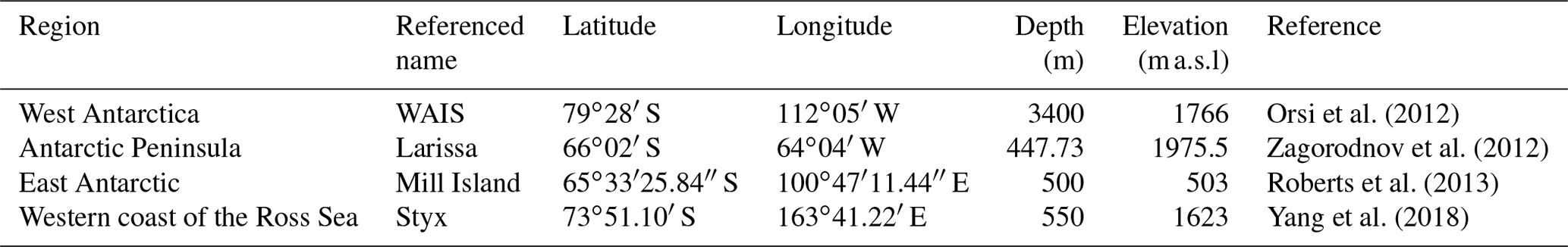
The data used in this study include measured temperature in four boreholes in Antarctica. We refer to them as West Antarctic Ice Sheet – “WAIS”, “Larissa”, “Mill Island”, and “Styx”. Figure 1 and Table 1 provide their locations and corresponding references. The borehole temperature profiles were sampled in January 2008 and January 2009 (WAIS), December–February 2009/10 (Larissa), the summer of 2009/10 (Mill Island), and the summer of 2014/15 (Styx). As shown in Fig. 1 (in red rectangles), the borehole temperature is affected by the seasonal cycle in the upper 15 m (Bodri and Cermak, 2011, chap. 1), which is not adequate for the reconstruction of annual mean surface temperature. Consequently, only depth under 15 m is used to reconstruct the surface temperature history and to compare with simulated borehole temperature profiles.

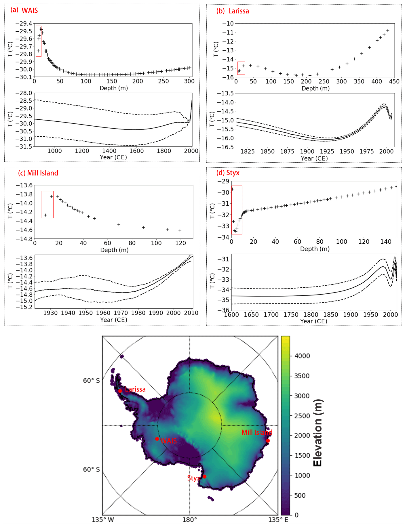
Figure 1 The observed borehole profiles and corresponding surface temperature reconstructions at the four sites in Antarctica. The symbols (+) show the measured borehole temperature. The dashed lines represent the reconstructed uncertainty, and the thick black lines are the mean reconstructed temperature. In panels (a), (b), (c), and (d), the red rectangles represent the borehole temperatures that are influenced by the seasonal cycle. The bottom panel shows the location of these four boreholes and their corresponding elevation over Antarctica.

Table 1 Location of the four boreholes. Elevation is in meters above sea level (m a.s.l.). Depth is in meters (m).

The temperature reconstructions and their uncertainty estimates for the four boreholes are shown in Fig. 1. For WAIS, Mill Island, and Styx, the reconstructed surface temperature series (Fig. 1a, c, d) are computed using a generalized least-squares algorithm (e.g., Orsi et al., 2012). For Larissa, the surface temperature is recovered by the Tikhonov regularization algorithm (Zagorodnov et al., 2012). This method has been proven to be valid for inverse problems such as the reconstructions based on borehole temperature observations, and the details of this method are explained in Nagornov et al. (2001, 2006). Since the temperature reconstructions are sensitive to the technique used, when we drive the borehole temperature model selected in this study by the published reconstructed temperature histories and compare them to the observed borehole temperature, differences are found. They are likely attributed to the different methodology and hypothesis. However, they are relatively small (Fig. S6 in the Supplement), suggesting that they do not have a major impact on the final conclusions.

2.2 Climate model simulations

The simulated surface air temperature used in this study (Table 2) is extracted from general climate model (GCM) simulations covering the past millennium performed in the framework of the third phase of the Past Model Intercomparison Project (PMIP3; Otto-Bliesner et al., 2009) and the fifth phase of the Coupled Model Intercomparison Project (CMIP5; Taylor et al., 2012). These simulations cover the period 850–1850,CE (referred to as the past1000 experiment in CMIP/PMIP nomenclature) and the years 1850–2005 CE (historical period). For the majority of the models, the simulations start thus in 850 CE and finish in 2005 CE. However, for two of the models, CESM1-CAM5 (Otto-Bliesner et al. 2016) and MPI-ESM-P (Stevens et al. 2013), the historical simulations covering 1851–2005 CE were performed independently of the simulations covering 850–1850 CE. In order to obtain results over the full millennium, we adopt the approach from Klein and Goosse (2018) and merge the first ensemble members (r1i1p1) of the past1000 experiment with the corresponding ensemble members of the historical experiment. Although not continuous, there is no large discrepancy in 1850 CE between the two merged simulations (e.g., Klein and Goosse, 2018).

Table 2 Climate model simulations used to drive the forward model.

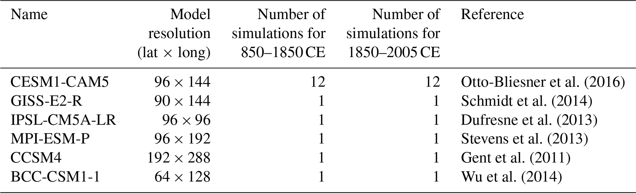
These simulations are driven by natural (orbital, solar irradiance, volcanic) and the anthropogenic (well-mixed greenhouse gases, ozone, aerosols, land use/land cover) forcings (Schmidt et al., 2011, 2012). Note that BCC-CSM1-1 and IPSL-CM5A-LR ignore the impact of land use/land cover, and IPSL-CM5A-LR does not consider any variations in aerosols and tropospheric ozone. Further description of the simulations and the forcing can be found, for instance in Klein et al. (2016). For CESM1-CAM5, it produces 12 different simulations with the same physics and same input forcings but slightly different initial conditions in the model. Therefore, the differences between ensemble members attributable to the process internal to climate system provide an estimate of the internal variability. For CCSM4, GISSE2-R, IPSL-CM5A-LR, MPI-ESM-P, and BCC-CSM1-1, there is only one simulation available. In addition, although we can obtain the simulated surface mass balance (SMB) from these models (e.g., Dalaiden et al., 2020), we do not use it here and keep the observed accumulation rate in the forward model, since biases in the simulation of SMB may affect our conclusions, and the focus here is on the simulated temperature evolution.

2.3 The forward model description

The forward model used herein to simulate the propagation of the signal coming from the surface temperature history into the subsurface is based on the one-dimensional heat and ice flow equation (Alley and Koci, 1990):

$$\begin{array}{}\text{(1)}& \mathit{\rho }{c}_p{\displaystyle \frac{\partial T}{\partial t}}={\displaystyle \frac{\partial }{\partial z}}\left(k{\displaystyle \frac{\partial T}{\partial z}}\right)-\mathit{\rho }{c}_{p}w{\displaystyle \frac{\partial T}{\partial z}}+Q,\end{array}$$

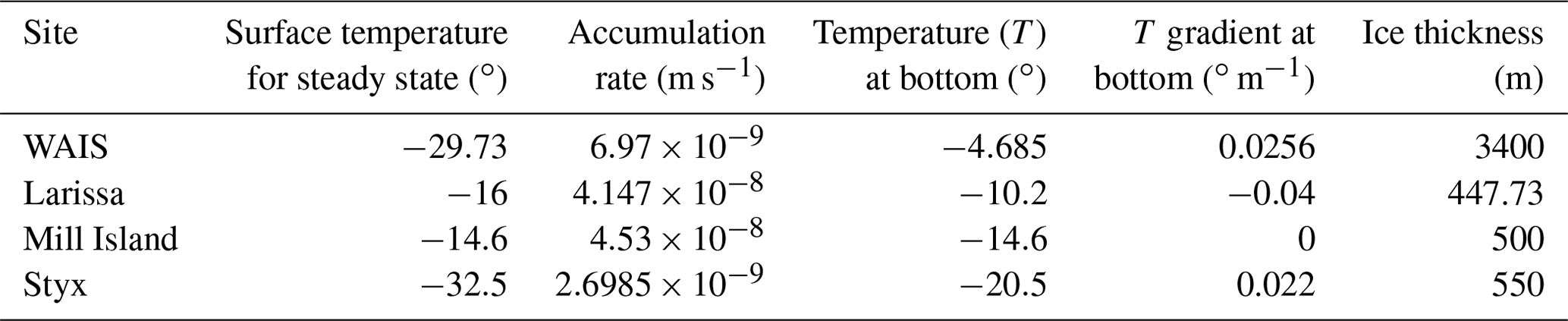
where T is the temperature, t is the time, c_p is the heat capacity, ρ is the density of firn/ice, z is the depth, w is the downward velocity of the firn/ice, and Q is the heat production term. In the Eq. (1), the term on the left side represents the change in heat content. On the right side, the first term corresponds to the rate of temperature change due to conduction based on Fourier's law. Ice moving vertically (z direction) with downward velocity, w, conveys a heat flux ρc_pwT across a plane of unit area, oriented perpendicular to z, which is accounted for in the heat transfer by advection shown as the second term. The third term, Q, consists of two parts: (1) ice deformation (Cuffey and Paterson, 2010, chap. 9, Eq. 9.30) and (2) firn compaction (Cuffey and Paterson, 2010, chap. 9, Eq. 9.33). Important model parameters are obtained from the references given in the Table 1, and they are summarized in Table 3. A detailed description of the model is available in the Supplement.

Table 3 Optimal parameters used to simulate subsurface temperature profile in the forward model driven by the reconstruction for each site: (a) WAIS, (b) Larissa, (c) Mill Island, and (d) Styx.

2.4 Sensitivity of subsurface temperature to model parameters

According to the original studies describing the records and the surface temperature reconstructions, the various parameters in the forward model have effects of different magnitude on the results for the different sites. Consequently, in order to assess the uncertainty in the model–data comparison related to the parameters of the forward model, we perform a series of sensitivity experiments on the parameters which have been shown to have the largest effects on each of the borehole profiles shown in the Fig. 2.

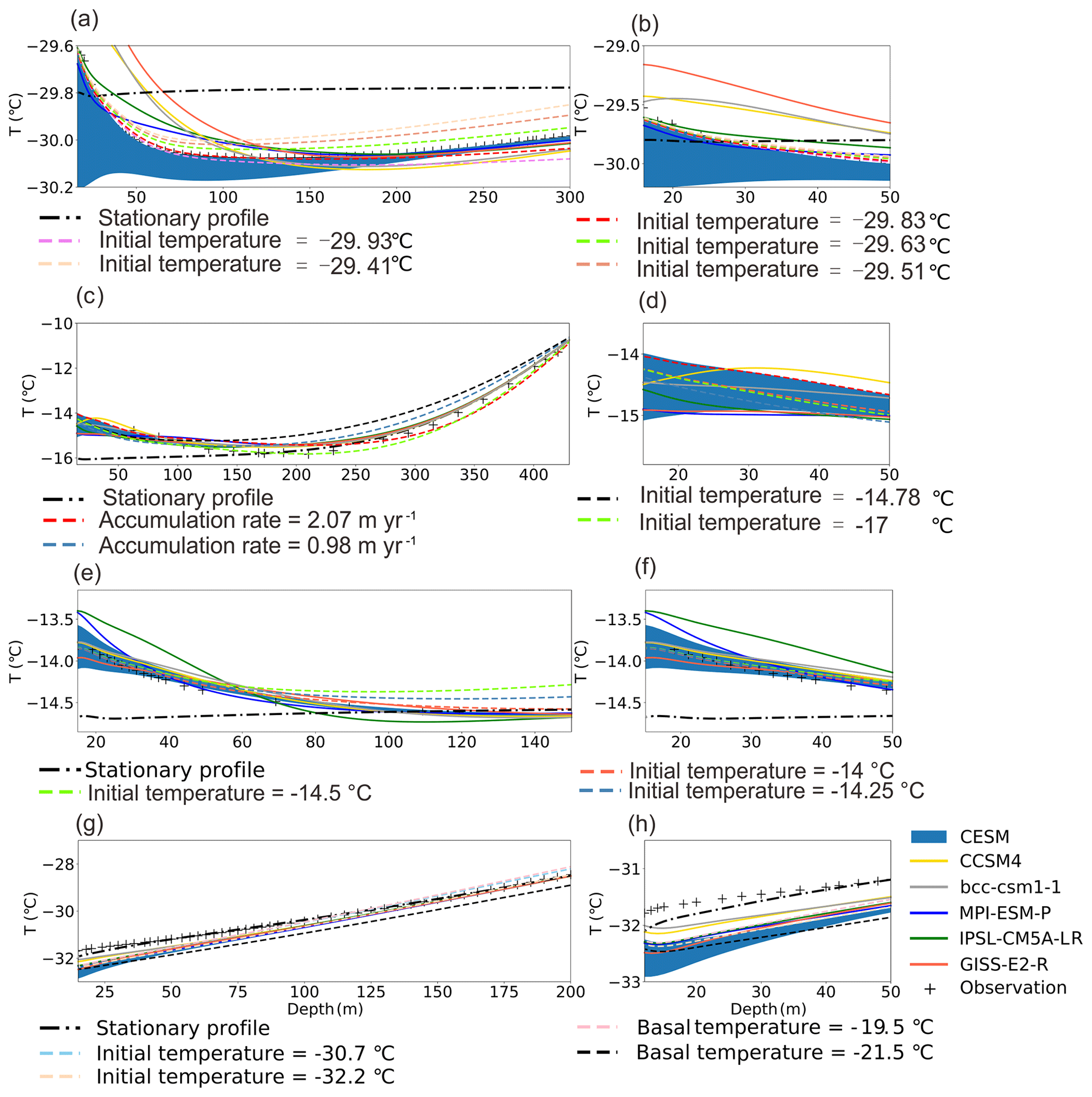
Figure 2 Comparison of borehole temperature profiles outputs for the forward model driven by GCM surface-temperature time series with optimal parameters (solid lines), and sensitivity tests using the temperature history of one CESM member (dashed lines) at each site. (a) WAIS: 15–300 m; (b) WAIS: 15–50 m; (c) Larissa: 15–430 m; (d) Larissa: 15–50 m; (e) Mill Island: 15–150 m; (f) Mill Island: 15–50 m; (g) Styx: 15–200 m; (h) Styx: 15–50 m. The shaded area represents the simulated subsurface temperature ensemble driven by CESM using optimal parameters. The thick dash–dot line denotes the stationary profile at each site.

At WAIS, the spread of the sensitivity tests is lower than the spread in the simulated borehole profiles driven by different climate model results (solid lines in color in Fig. 2a and b). However, the initial temperature derived from a steady-state profile has an influence on the slope of the profile in the deeper part and on the depth of the temperature minimum, contributing to the uncertainty in the intensity of the pre-1900 cooling trend and the timing of the temperature minimum.

At Larissa, the effect of the bottom boundary conditions is important in setting up the temperature gradient from the bottom to 300 m, and therefore, we will not interpret that segment of the data in terms of climate. It is also evident in Fig. 2c that the different temperature histories produce a very similar depth profile over that interval.

At Mill Island, the borehole profile is shallow and covers only a fraction of the full thickness of the ice sheet. At sites with such a deep ice sheet and with a high accumulation rate, the optimal surface temperature history was found to be essentially independent of the location of the imposed bottom boundary condition for depths in excess of 180 m below the surface (Roberts et al., 2013). Consequently, here we modeled the temperature by assuming a zero-heat-flux bottom boundary. Although the initial temperature has an influence on the slope of the profile deeper than 120 m, this sensitivity is weak in depths shallower than 80 m, and the borehole profile is dominated by the surface temperature history.

At Styx, the bottom boundary condition is adjusted to reproduce the slope of the temperature profile in the deeper part (100–200 m). The simulated borehole profiles driven by GCMs (solid lines in the Fig. 4e) show the large deviation in the top 100 m compared to stationary temperature profile, which suggests that there is climate information stored in the upper part of the profile. Meanwhile, at depths shallower than 50 m, the effect of boundary conditions is weaker than the differences in the temperature histories from the different models, which means the borehole temperature data can be used to discriminate between temperature histories provided by the different models.

The internal variability also has a significant impact on the shape of the simulated borehole profiles. At these four sites, the range of simulations driven by CESM ensemble is much larger than the range of the different sensitivity tests in the top 50 m (shown as the shaded area in Fig. 4b, d, f, and h). This confirms that internal variability is a dominant source of uncertainty in a model–data comparison, at least in the top 50 m. For the deeper part of WAIS, as the shape of subsurface temperature profiles is influenced by the parameters of the forward model, the evaluation of the long-term cooling trend is more uncertain.

3 Results

3.1 Comparison between the simulated temperature and reconstructions

Figure 3 displays the comparisons between climate model results and temperature reconstructions from the boreholes. The simulated temperatures displayed in Fig. 3 come directly from the surface temperature calculated by the climate model, based on its own dynamics and the forcing applied as discussed in Sect. 2.2. In order to ensure that the climate model results have the same mean over the reference period (which is the whole period derived from the reconstruction) as the reconstruction, we applied a very simple, constant correction to remove the mean bias of the climate model results as shown in the Fig. 3. Due to the nature of physical diffusion, the heat propagation acts similarly to a low-pass filter. The reconstructions thus suffer from an attenuation of high-frequency temperature variability that becomes stronger as time goes back (Beltrami et al., 2006; Harris and Gosnold, 1999). For instance, in the reconstructed surface temperature of Styx, the point corresponding to 1800 CE in the curve may represent an average temperature between around 1600 and 1900 CE, while in 1900 CE it corresponds to an average over around 200 years. This characteristic complicates the model–data comparison. Therefore, in order to facilitate the comparison between the reconstruction and climate model results, we use variable smoothings to mimic the characteristic as much as possible. Since the reconstructions have much wider ranges than those ones from the climate model results, the basic compatibility between model and data will not be changed due to various smoothing. Nevertheless, Fig. 3 must be interpreted carefully because of this inhomogeneous smoothing.

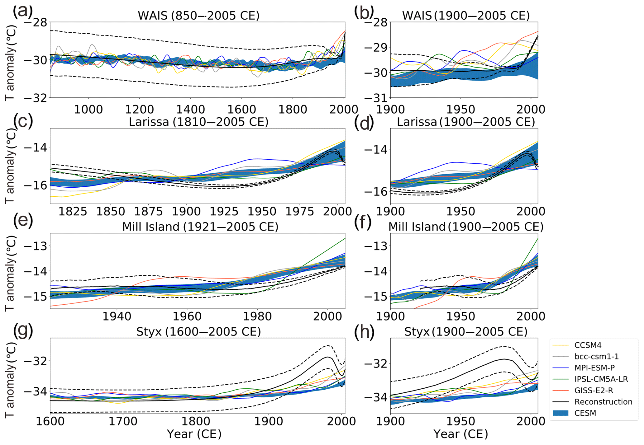
Figure 3 Comparison between reconstructed surface temperature series from boreholes and the climate model outputs at the grid cell closest to each borehole site. The borehole reconstructions are in black and their uncertainty ranges given by the dashed lines. Color lines correspond to the climate model results. The shaded area represents the mean ±1 standard deviation of CESM model ensemble. For the left column, a 50-year LOWESS has been applied for the WAIS and Styx time series; Larissa and Mill Island are smoothed using 10- and 3-year windows, respectively. The time series in the right column is smoothed using 3-year windows from 1900 to 2005 CE.

Because of the internal variability in the system, a single simulation without error bound is not expected to reproduce well all the characteristics of the observed variations. The difference can be large, in particular at the local level (e.g., Goosse et al., 2005), but the observations should correspond to a credible member of an ensemble of simulations. Ensuring this compatibility can be achieved using various techniques, but the first step is to simply check if the reconstruction is within the range provided by the ensemble (e.g., PAGES2k-PMIP group, 2015).

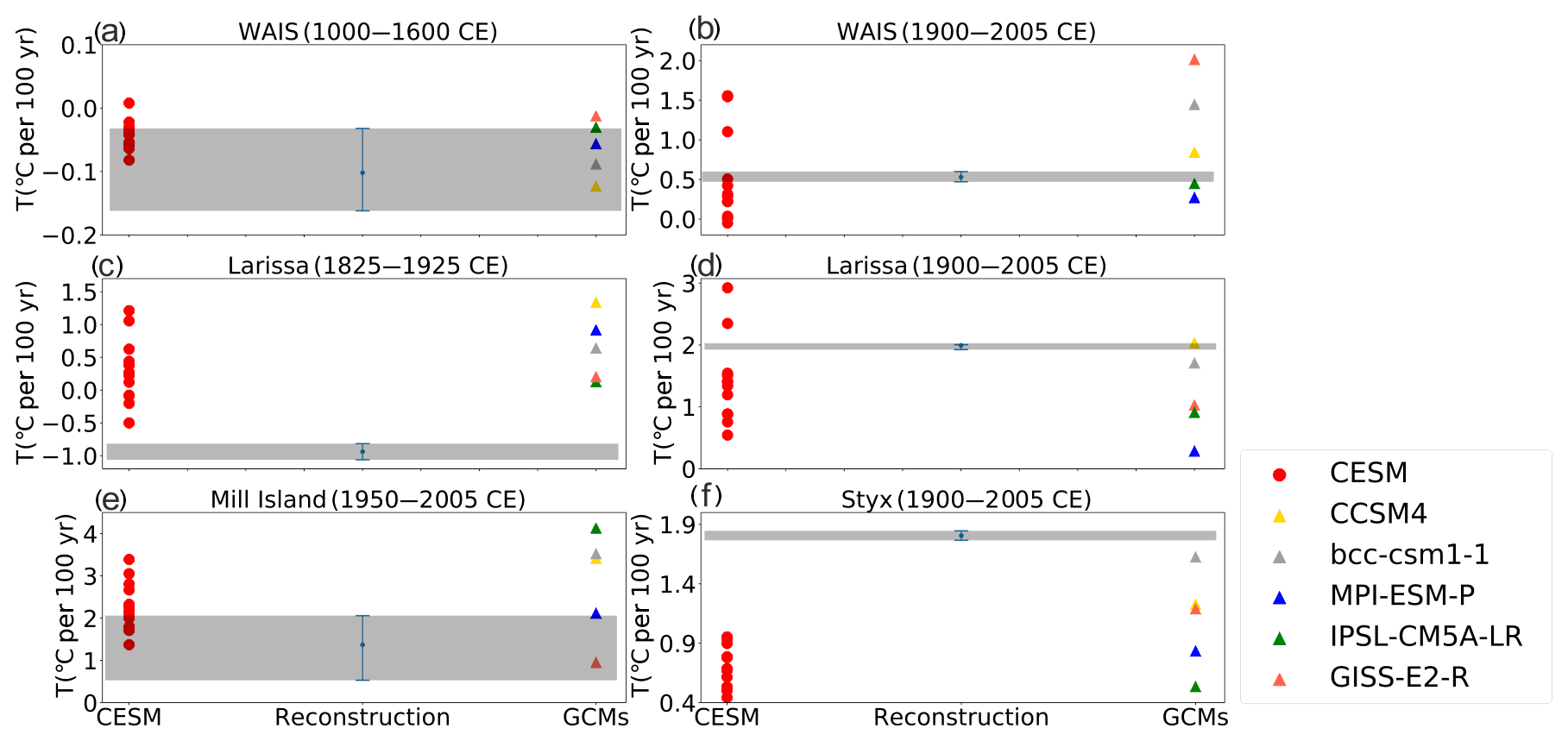
Figure 4 Linear trends for the four boreholes over different periods: (a) WAIS: 1000 to 1600 CE; (b) WAIS: 1900 to 2005 CE; (c) Larissa: 1825 to 1925 CE; (d) Larissa: 1900 to 2005 CE; (e) Mill Island: 1950 to 2005 CE; and (f) Styx: 1900 to 2005 CE.

Considering the large uncertainty range in these reconstructions, the climate models are visually able to reproduce the general characteristics of reconstructed temperature variability, particularly the long-term cooling during the last millennium and the recent warming (Figs. 3 and 4). Nevertheless, disagreements have also been identified.

The first major feature in the data is this long-term cooling trend, visible at the WAIS and Larissa sites. At Larissa, the borehole temperature reconstruction gives a cooling trend of $-\mathrm{0.94}\pm \mathrm{0.12}$ ^∘C per century from 1825 to 1925 CE (Zagorodnov et al., 2012). None of the models are able to reproduce this observation, and instead, they all show a warming trend of comparable magnitude (Figs. 3c and 4c). At WAIS, the borehole temperature inversion also shows a long-term cooling trend, from 1000 CE to about 1600 CE, with a magnitude of $-\mathrm{0.10}\pm \mathrm{0.07}$ ^∘C per century (Fig. 3a). The large uncertainty in the long-term trend is principally due to the uncertainty in the initial surface temperature (Fig. 2a; Orsi et al., 2012, their Fig. 3). The quantitative comparison between the trend of reconstructions and climate model outputs (Fig. 4a) indicates that the simulations generally show a cooling trend over 1000–1600 CE, in agreement with previous studies (e.g., Goosse et al., 2012; Abram et al., 2016; Klein et al., 2019). The amplitude of the trend is lower, particularly for GISS (−0.01 ^∘C per century) and IPSL (−0.03 ^∘C per century) models, but most remain within the lower end of the reconstructed uncertainty range. This long-term cooling trend is a feature of the Antarctic climate that is visible in many other ice core records (Stenni et al., 2017). A recent compilation of PAGES Antarctica2k datasets calculated a trend of −0.26 to −0.4 ^∘C per 1000 years for the period 0–1900 CE for the Antarctic continental average (Stenni et al., 2017). In the high latitudes of the Southern Hemisphere, the origin of this millennial-scale cooling is currently not well understood, but an intermediate complexity model has shown multimillennial cooling in summer because of a delayed response to the decrease in local spring insolation (Renssen et al., 2005) with an additional potential influence of volcanic forcing (Goosse et al., 2012; Abram et al., 2016; Stenni et al., 2017).

A second feature of the data is a warming trend in the 20th century, which started at different times in the different records. Styx shows an early warming trend from 1900 to 1980 CE and a general stabilization of the temperature afterwards (Fig. 3h). This signal is consistent with the data from weather stations and ice core isotope-derived records (Yang et al., 2018). Models tend to show the opposite timing, with nearly no trend from 1900 to 1960 CE and a late warming trend that differs in amplitude between models. Overall, the simulated warming of the 20th century is about half of what is observed (Fig. 4f), with BCC (1.63 ^∘C per century) and CCSM4 (1.23 ^∘C per century) having the largest trends, closest to the observations (1.81 ^∘C per century).

Larissa shows a temperature minimum in 1940s, followed by a steady warming trend until around 1995 CE. The magnitude of the 20th-century trend is 1.99 ^∘C per century. Most models reproduce the timing of the warming reasonably well, with the exception of MPI, which shows an early warming, but no trend in 1940–2005 CE, and GISS, which has a very muted trend. If the trend present in the other models is too low, it seems rather due to a lack of cooling in the preceding century than because of errors in the latest decades.

Mill Island shows a late warming trend starting in the 1980s. Models tend to overestimate this trend (Fig. 4e), in particular IPSL, BCC, and CCSM4. Similarly to Mill Island, WAIS also shows a positive trend over the period 1900–present that intensifies after 1980 CE. The amplitude of the 20th century warming (0.53 ^∘C per century) is well simulated, but the start of the trend occurs sometimes too early, with the exception of CESM, BCC, and IPSL, which show a late warming trend (Fig. 3b).

Overall, for WAIS (Fig. 4b) and Larissa (Fig. 4d), the reconstructed trends lie in the CESM ensemble range, suggesting many apparent model disagreements for those sites can be due to internal variability. For Styx (Fig. 4f) and Mill Island (Fig. 4e), the reconstructed trends are larger than the spread of the CESM ensemble, which means the disagreements are not only due to internal climate variability but also related to a systematic climate model bias in this region.

However, as stated above, borehole temperature reconstructions are “underdetermined”, which means that there are many possible temperature histories that can fit the data (more detailed explanation of underdetermined is given in the Introduction). The next step is to determine if the differences between simulated and reconstructed time series can be discriminated when analyzing observed and simulated temperature profile.

3.2 Comparison of the simulated subsurface temperature with observation

The simulated subsurface temperature profile is the results of the superposition of two components: (1) the initial temperature profile that incorporates the effects basal heat flux and vertical advection due to ice accumulation and (2) the subsurface temperature deviations arising from the surface temperature variability. Since the initial temperature profile for each borehole is obtained by driving the forward model with the optimal parameters obtained from the original publications (see Sect. 2.4), the differences among the simulated borehole profiles for each location are caused only by the changes in the upper boundary, i.e., in the climate model outputs. The simulated subsurface temperature profiles for each borehole are displayed in Fig. 5.

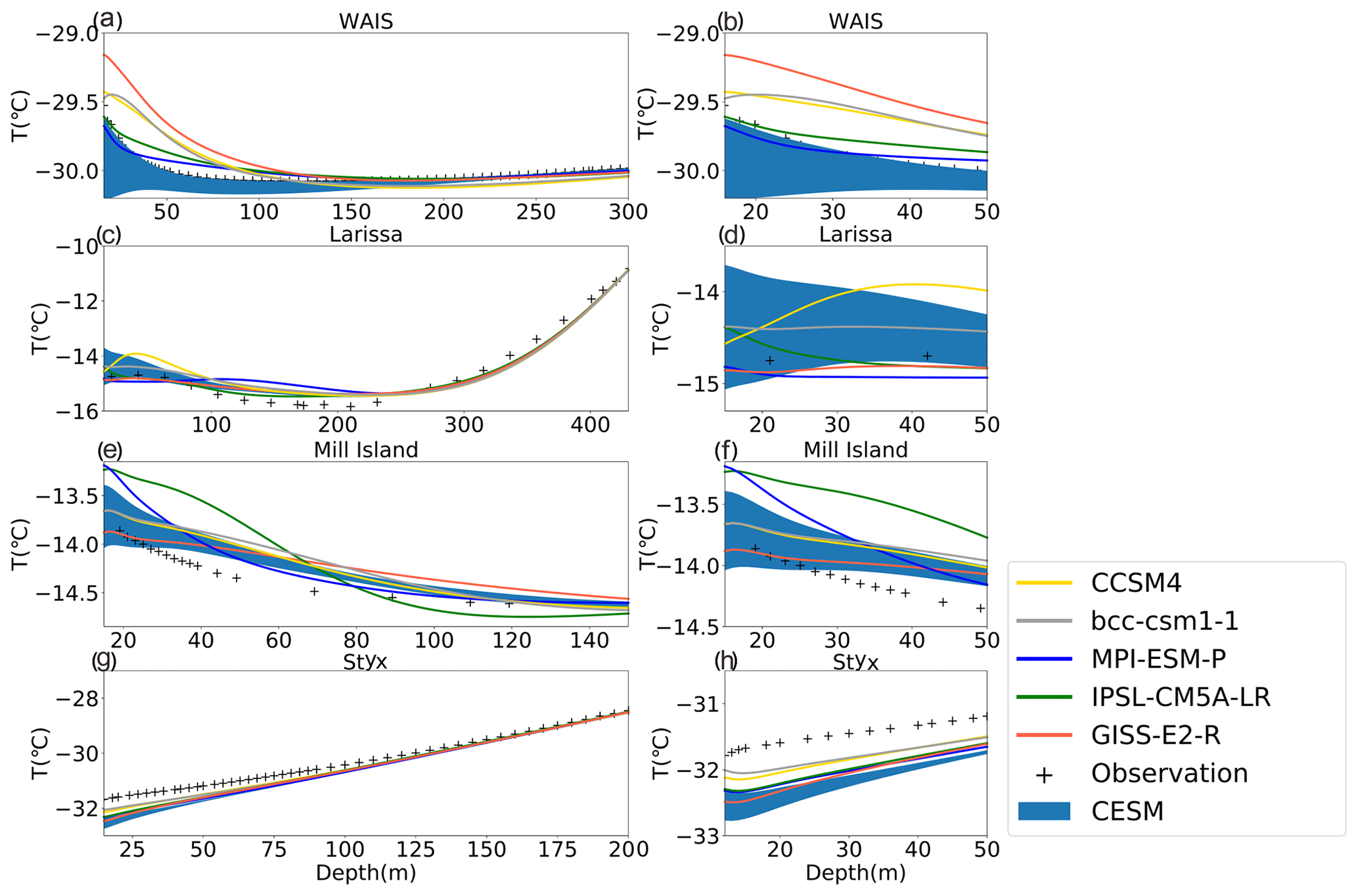
Figure 5 Comparisons between simulated subsurface temperature and measurements for the following: (a) WAIS: 15–300 m; (b) WAIS: 15–50 m; (c) Larissa: 15–430 m; (d) Larissa: 15–50 m; (e) Mill Island: 15–150 m; (f) Mill Island: 15–50 m; (g) Styx: 15–200 m; and (h) Styx: 15–50 m. The shaded area represents the simulated subsurface temperature ensemble driven by CESM ensemble. The right column is a zoom over the upper 50 m for each borehole.

As previous studies have shown (e.g., Bodri and Cermak, 2011, chap. 2), a “U”-shaped subsurface temperature profile is a direct evidence for the past climate change with a minimum that separates the deeper warming trend due to geothermal heating and shallower warming trend related to a recent temperature increase (Orsi et al., 2012; Stevens et al., 2008). Among these four sites, WAIS and Larissa have such characteristics of a U shape. For Mill Island, this is less clear, but a significant breaking point in each simulated subsurface temperature profile reflects the surface temperature warming over recent decades. For Styx, such a break does not seem to be present at all, and the slope does increase with depth.

Aided by these key properties, we can identify a link between the interpretation in the depth domain and in the time domain. The analysis of the simulated and observed temperature profile confirms the main conclusion obtained in Sect. 3.1, in particular the agreement between model and data on the general tendencies, characterized by a long-term cooling trend over last millennium and the recent warming. For the deeper part of the profile, the simulated temperature profiles driven by MPI, IPSL, and GISS at WAIS almost coincide with the corresponding observation, but they fail to reproduce the depth of the temperature minimum around 120 m in the data. This is consistent with the fact that IPSL and MPI are at the edge of the reconstructed cooling trend of the last millennium, and GISS presents a significant underestimation of this trend (Fig. 4a). However, the CESM ensemble follows the borehole temperature profile (shaded area in Fig. 5a) and can also reproduce the magnitude of the cooling trend for some of the members (Fig. 4a). Specifically, the minima in the simulated profiles driven by MPI, IPSL, GISS, and CESM are −30.06, −30.06, −30.07^∘, and a range of −30.8 to −30.17^∘, respectively, which is very close to the minimum of −30.08^∘ in the observation.

At Larissa, the bottom (270–450 m) of the profile is controlled by boundary conditions (Fig. 2c) and contains no climate information, as demonstrated by the fact that all curves are on top of each other in Fig. 5c. Additionally, no simulation has a pronounced inflection point around 170 m as shown in the observation. These characteristics are perfectly consistent with the lack of a cooling trend from mid ∼ 19th century to the early 20th century in the simulations (Fig. 3c). We conclude from this that the cooling trend of 1825–1925 CE is a robust feature in the data that can be used to benchmark climate models.

For the recent warming, we see some significant discrepancies among the simulated subsurface temperature profiles driven by different climate models at the four boreholes in the depth domain that are consistent with the signal analyzed in the time domain. For WAIS, in the uppermost part, the simulated subsurface temperature profiles driven by GISS, CCSM4, and BCC display significantly higher temperature than those in the observations, while IPSL and MPI-simulated profiles are close to the observations (Fig. 5b). This is in perfect agreement with the too high temperatures in models compared to the reconstructions in the second half of the 20th century (Fig. 3b).

For Larissa, all simulated profiles display an increasing temperature toward the surface as in observations but with different magnitude and shape (Fig. 5c). The temperature in the simulation driven by MPI displays a relatively rapid increase until around 100 m and then is constant, which is consistent with the near-constant temperature from 1940 to 2005 CE (Fig. 3d). For the ones driven by CCSM4 and BCC, they are warmer than the observation between depths of 15 and 50 m, which reflects the consistently warmer temperature shown in Fig. 3d. The IPSL-simulated subsurface temperature profile displays the largest similarity to the observations, while the simulations performed with CESM can cover almost all the observation in the shallow zone.

For Mill Island, the simulated subsurface temperature profiles are warmer than observations above 50 m, confirming the too large a warming trend deduced from the analysis of surface temperature. In particular, the IPSL model has the largest warming trend (Fig. 3e and f) and also has the warmest temperature profile (Fig. 5e and f), followed by MPI. For Styx, the main discrepancies occur over the shallow depths, between of 15 to 60 m, where all the simulations depict colder conditions compared with observations (Fig. 5g and h), as for the surface temperature over the recent decades in Fig. 3.

We also find in the depth domain some signals that are not obvious in the time domain. In particular, for WAIS, one of the CESM runs matches the warming trend of the top 100 m, while in time domain the CESM ensemble is significantly colder than reconstruction over recent decades. The CESM outputs generally follow the data in the deeper part of the profile (200–300 m) and have an even steeper slope between 100 and 200 m (Fig. 5), while in the time domain, the cooling trend was underestimated (Fig. 4a). In addition, for WAIS, the simulated subsurface temperature profiles driven by CCSM4 and BCC over the deeper part of the profile are colder than observations, but the warming trend starts deeper, at about 200 m compared to 120 m in the observations. This seems puzzling because, in the time domain, the cooling trend continues until 1800 CE for CCSM4 (Fig. 2a, yellow). However, the larger warming in the last 100 years is probably shifting the temperature minimum downwards. This example shows that it is difficult to pinpoint the date corresponding to a temperature minimum in the depth profile, because it depends on the respective speed of warming and cooling before and after. At Mill Island, in the deeper part (around from 140 to 100 m) of the profile, the simulated subsurface temperature profile driven by IPSL is very different from the other ones, with a slightly decreasing temperature and a colder climate than observations. However, in the time domain, the difference compared to other time series for IPSL was much less clear (Fig. 3e), but the consistency between these two domains still exists, and especially the temperature minimum in 1980 CE might correspond to the deeper part (around 100 m) in the depth domain.

The comparison between the analyses in the two domains appears thus complementary and instructive as it illustrates that the interpretation may be easier in one case or the other. It also shows that the observations can help evaluate the models by comparing different borehole temperature profiles driven by the different climate model results with the corresponding observation. In particular, the analysis of the simulated temperature profiles confirms that CESM ensemble can reproduce the multidecadal and centennial climate variability at WAIS.

4 Proposed metric of Antarctic climate for model validation

In this section, we use the results of the previous section to describe a few metrics that can be used easily to evaluate the next generation of climate model simulations (e.g., PMIP4-CMIP6; Jungclaus et al., 2017) and investigate the spatial representativity of the records.

4.1 Metric 1: last-millennium cooling at WAIS

Of the four records presented here, WAIS has the longest retrievable history. We propose here to use the temperature trend of the period of 1000 to 1600 CE as a metric, with the magnitude of $-\mathrm{0.102}\pm \mathrm{0.07}$ ^∘C per century (Fig. 4a). The end of the cooling trend is not clearly defined by the data, due to the complex time-varying smoothing of the borehole temperature record, but 1600 CE seems to be safely in the cold interval (See Orsi et al., 2012, for details). The start of the period is more open, and we chose 1000 CE to be compatible with last-millennium simulations. External evidence from a compilation of water isotope records indicates that the cooling trend extended likely from 0 to 1900 CE in many parts of Antarctica (Stenni et al., 2017). It is a robust feature of the Antarctic climate of the last 2 kyr, and the WAIS record is unique in providing a clear quantification of the temperature trend.

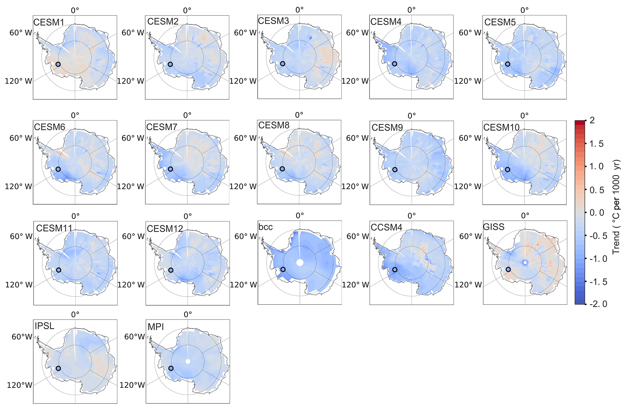
Figure 6 The simulated (blue to red shaded area) and observed (circle) surface temperature trend from 1000 to 1600 CE in Antarctica.

Figure 7 The ratio of the surface temperature trend (blue to red shaded area) from 1000 to 1600 CE between other grid cells in Antarctica and WAIS. The black circle denotes the location of WAIS.

In Fig. 6, we show the 1000 to 1600 CE surface temperature trend at WAIS and at other sites in Antarctica from the models output. Visually, for most simulations, the cooling at the grid cell of WAIS is similar to the one obtained at many locations in West Antarctica. Only the first member of CESM shows a small warming trend in West Antarctica. The large spatial coherence of the trend indicates that, although we are making a single-point comparison, it represents a signal common to a large part of the continent. It is also important to estimate the magnitude of the trend at WAIS compared to other regions. To do so, we calculate the ratio of the trend of surface temperature from 1000 to 1600 CE at any location with the one at WAIS (Fig. 7). Except the first member of CESM, if the value is greater than 1 (shown in red tones), it means the trend at the grid cell is larger than that at WAIS; if the value lies between 0 and 1 (shown in blue tones), it means the trend at the grid cell is less than that observed at WAIS. Negative values (i.e., a trend of a different sign compared to WAIS) are not shown, and the corresponding region is blank. Since the goal of Fig. 7 is to show the intensity of cooling at WAIS compared with other points in Antarctica, the first member of CESM 1, which shows a warming trend close to zero at WAIS, is not very meaningful, but it is still included for completeness. Seventy-five percent of models show that WAIS displays larger cooling from 1000 to 1600 CE than other locations in Antarctica (shown in blue) but with magnitude similar to other grid cells in West Antarctica. This is consistent with the reconstruction of Stenni et al. (2017) that shows the largest cooling in this region over the period 0–1900 CE. The spatial patterns of the trends (Fig. 7) are different not only between models but also within the CESM ensembles, showing that the changes in Antarctica are strongly influenced by internal variability, even at the century timescale. Future work including more sites or using water isotopes and the Antarctica-2K database will help constrain the spatial pattern of this trend.

4.2 Metric 2: 19th century cooling at Larissa

The second metric is the surface temperature trend over the period from 1825 to 1925 CE at Larissa, with the magnitude of $-\mathrm{0.94}\pm \mathrm{0.12}$ ^∘C per century. Figure 8 shows the spatial correlation between the temperature from 1825 to 1925 CE at Larissa and other grid cells for each climate model. As there are no significant differences between each member in CESM ensemble (see in the Fig. S1), only one member of CESM1 is presented in the Fig. 8. Despite the correlation coefficient decreasing with the distance from the Larissa, the values are higher than 0.6, at least around Larissa, showing that this metric is representative of part of the AP region and not extremely site specific.

Figure 8 The correlation map (blue to red shaded area) showing the relationship between the temperature from 1825 to 1925 CE at Larissa and other grid cells in Antarctica for each climate model. The dashed black contour lines show a significant correlation at the 99 % significance level.

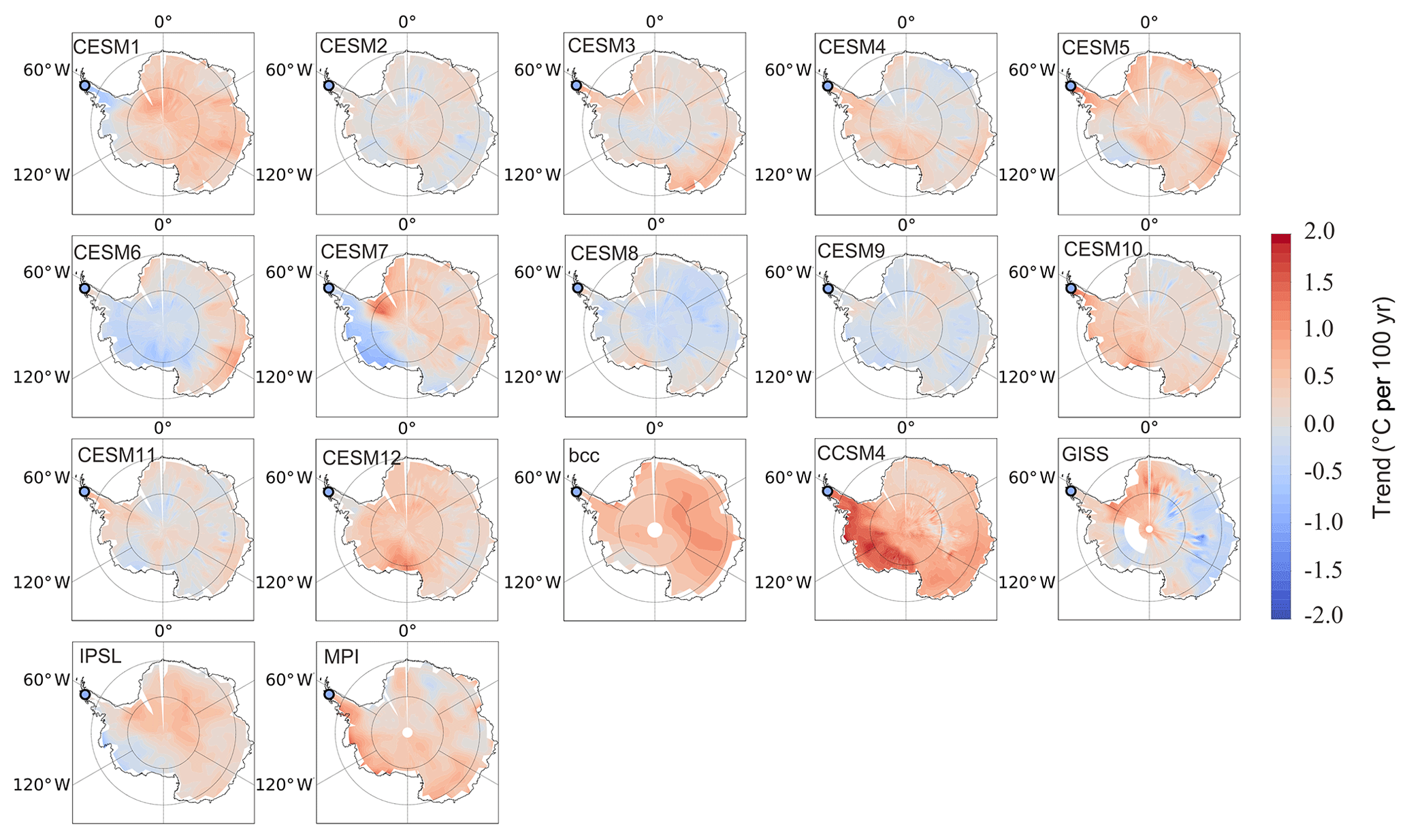
Figure 9 The simulated (blue to red shaded area) and observed (circle) surface temperature trend from 1825 to 1925 CE.

None of models are able to capture the observed temperature trend from 1825 to 1925 CE (Fig. 9). Overall, models are showing a warming trend (largest for CCSM4, MPI, and BCC), contradicting the observations, as highlighted already in Fig. 4c. Only four members of CESM (CESM1, 7, 8, and 9) show a cooling trend over AP, but their magnitudes are still less than the observed one.

The 19th century is a time period when the Northern Hemisphere has started warming, whereas Southern Hemisphere records (Neukom et al., 2014), specifically Antarctica, show no general warming trend (Stenni et al., 2017). Models tend to overestimate the interhemispheric synchronicity (Neukom et al., 2014) and show a warming trend also in Antarctica, possibly in response to the anthropogenic forcing. This metric is thus an important tool for future research to evaluate whether the model data mismatch is due to internal variability (which will be investigated with more ensembles of the same model) or to an overestimated sensitivity to the anthropogenic forcing.

4.3 Metric 3: recent warming trend

The warming trend of the last 50 years is one of the clearest features of the observations. Here we propose a metric of the warming trend from 1950 to 2005 CE at each of the four sites, to investigate whether model can reproduce these features.

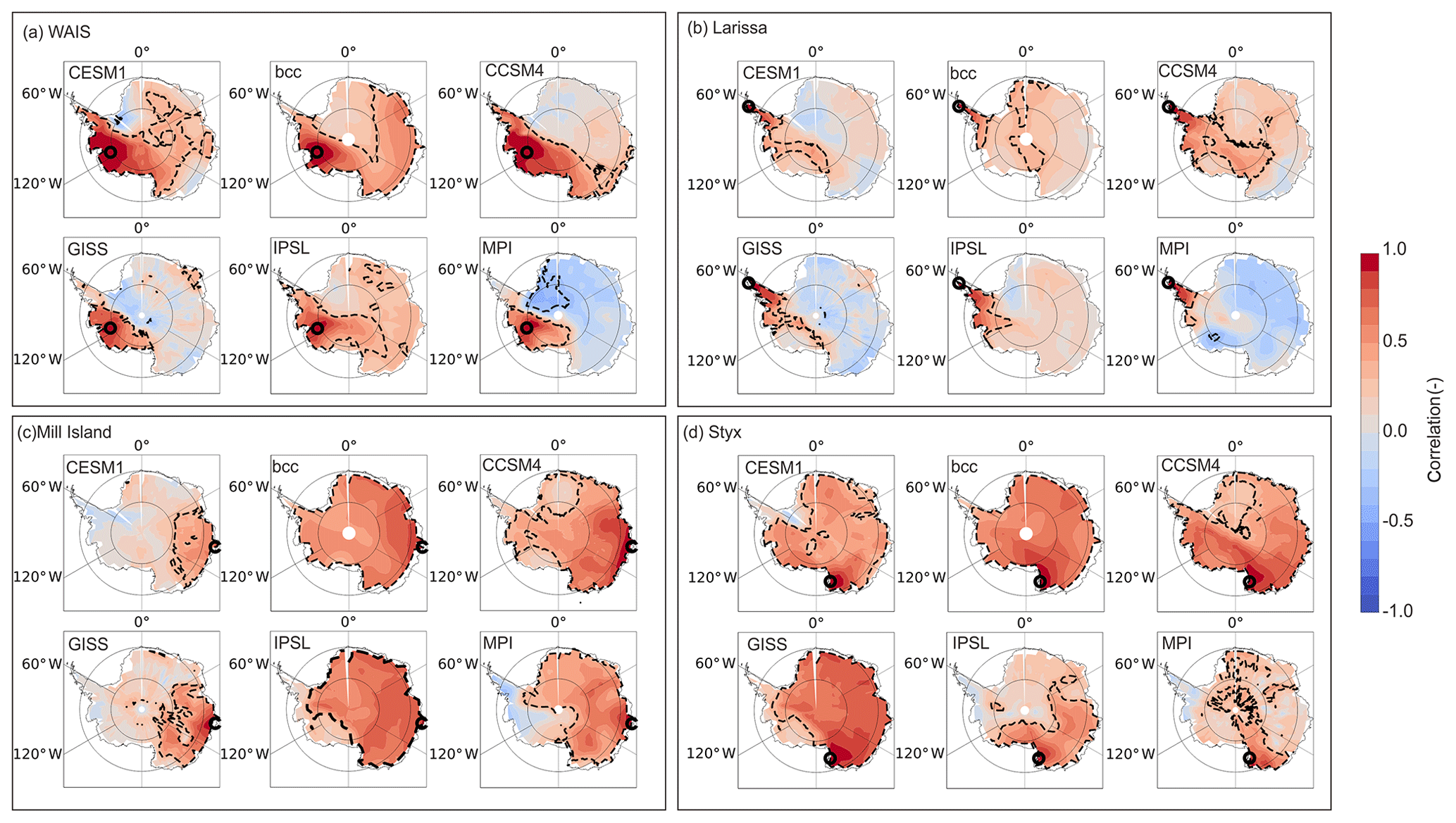
Figure 10 The correlation map showing the relationship between the temperature from 1950 to 2005 CE at (a) WAIS, (b) Larissa, (c) Mill Island, (d) Styx, and other grid cells for each climate models. The black contour lines show correlation at the 99 % significance level.

First we look at the spatial correlation of the temperature between each site and other grid cells for all GCMs (Fig. 10). Only one member of CESM1 is presented in the Fig. 10 since no significant difference is observed between each member in the CESM ensemble (see Figs. S2–S5). The correlation is calculated from annual data for 1950 to 2005 CE. It is clear that each of our borehole temperature sites gives information about different sectors of Antarctica. Generally speaking, WAIS is representative of the West-Antarctic continent, with a more pronounced dipole between WAIS and the Weddell Sea sector in MPI and, to a lesser extent, CESM and GISS. Larissa is representative of the AP as a whole, and from this resolution of climate model results, there is no evidence of a dipole between both sides of the Transantarctic Mountains. Similar to WAIS, MPI has the strongest expression of a dipole between the AP and East Antarctica, a feature that is weaker but also present in GISS. Mill Island is generally representative of the Wilkes Land sector of East Antarctica, with the largest spatial homogeneity for BCC and IPSL (Fig. 10c). Finally, for Styx, the models with the largest spatial homogeneity (BCC and IPSL) show a strong correlation between Victoria Land and the rest of East Antarctica.

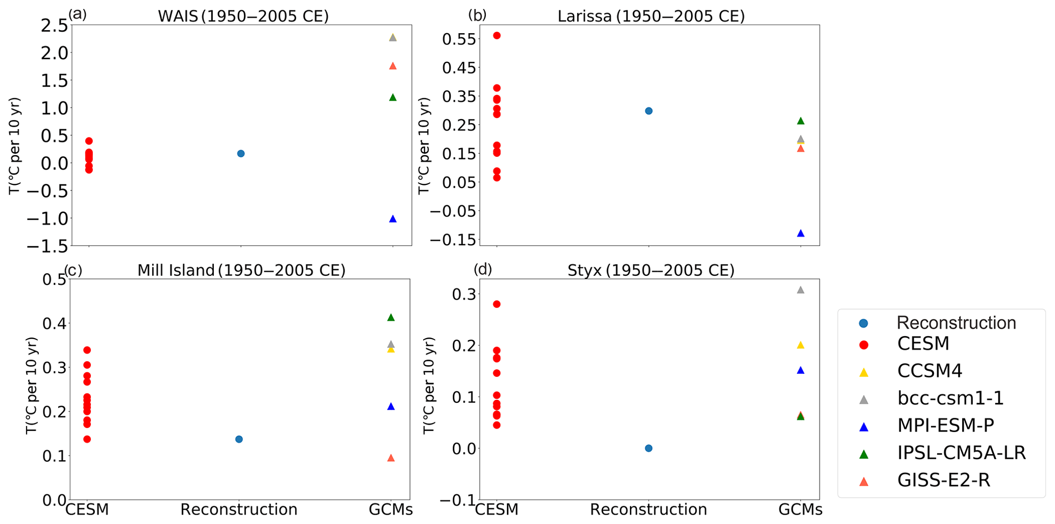
Figure 11 Linear trends for the four boreholes over 1950 to 2005 CE: (a) WAIS; (b) Larissa; (c) Mill Island; and (d) Styx.

Figure 11 shows the surface temperature trend from 1950 to 2005 CE. The strong warming trend at Larissa is underestimated in all the models except the CESM ensemble (Fig. 11b). Additionally, 3 out of 12 CESM simulations indicate cooling in West Antarctica, which is coherent with the hypothesis that the part of the observed warming is due to unforced variability and that models are not expected to match this trend perfectly. The warming at Mill Island is relatively well reproduced. However, none of the models can reproduce the muted recent warming seen at Styx. The lower spatial representativity of this site (Fig. 10) leads us to interpret this as local processes missing in low-resolution GCMs, such as the influence of topography on katabatic wind forcing, rather than a large-scale failure of models to represent reality.

5 Conclusion

In this study, we test two complementary ways to evaluate the climate model performance using borehole temperature observations. The standard way is to compare the reconstruction of surface temperature with simulated values in the time domain. The successful application here of a forward model driven with climate model results provides an additional way to analyze jointly model results and borehole temperature measurements. Compared to the model–data comparison in the time domain, the forward model allows us to reproduce the subsurface temperature profiles and to compare them directly with measured borehole temperature profiles.

The comparison of the surface-temperature time series is simpler and more straightforward, but it is limited by the different resolutions of the reconstructions and climate model results. Nevertheless, some robust conclusions can be derived from this model–data comparison that is confirmed by the direct analyses of the temperature profiles as a function of the depth. For instance, the long-term cooling trend over the last millennium observed at WAIS is relatively well reproduced in all models but with a weaker amplitude, which means the model maybe miss some feedbacks or low-frequency internal variability. Most simulations agree with data on a recent warming, but the magnitude and timing vary a lot between models for the four sites. The large variability in the trends over the 20th century within the CESM ensemble for WAIS and Larissa suggests that many apparent model disagreements for those sites can be due to internal variability, while the disagreement for Styx and Mill Island may be related to local processes not captured by global models.

The comparison of the model output and data in the depth domain is useful because the borehole temperature inversion is an underdetermined problem, and many different temperature histories could fit the data equally well. The comparison of the temperature profiles confirms the conclusions found in the time domain and validates the significance of some of the differences found. Some features are, however, difficult to interpret, such as the depth of the temperature minimum at the WAIS site. This points to the complexity of the interpretation of the borehole profiles and the complementary use of the analyses in the depth and time domain.

Finally, some metrics derived from the corresponding reconstructions are proposed to be used more widely in model evaluation. The metrics used are demonstrated to be generally representative of a large spatial area, although they are calculated at a specific site. The results confirm that no models can reproduce the cooling during 19th over the AP and a stabilization of the temperature over last 50 years in northern Victoria Land. Nevertheless, these models can capture the larger long-term cooling from 1000 to 1600 CE in West Antarctica and the recent 50 years of warming in West Antarctica and the AP. This work brings quantitative tools to evaluate models and better simulate the Antarctic climate and its response to forcings.