Dynamical and hydrological changes in climate simulations of the last millennium

Simulations of climate of the last millennium (LM) show that external forcing had a major contribution to the evolution of temperatures; warmer and colder periods like the Medieval Climate Anomaly (MCA; ca. 950–1250 CE) and the Little Ice Age (LIA; ca. 1450–1850 CE) were critically influenced by changes in solar and volcanic activity. Even if this influence is mainly observed in terms of temperatures, evidence from simulations and reconstructions shows that other variables related to atmospheric dynamics and hydroclimate were also influenced by external forcing over some regions. In this work, simulations from the Coupled Model Intercomparison Project Phase 5 and Paleoclimate Modelling Intercomparison Project Phase 3 (CMIP5/PMIP3) are analyzed to explore the influence of external forcings on the dynamical and hydrological changes during the LM at different spatial and temporal scales. Principal component (PC) analysis is used to obtain the modes of variability governing the global evolution of climate and to assess their correlation with the total external forcing at multidecadal to multicentennial timescales. For shorter timescales, a composite analysis is used to address the response to specific events of external forcing like volcanic eruptions. The results show coordinated long-term changes in global circulation patterns, which suggest expansions and contractions of the Hadley cells and latitudinal displacements of westerlies in response to external forcing. For hydroclimate, spatial patterns of drier and wetter conditions in areas influenced by the North Atlantic Oscillation (NAO), Northern Annular Mode (NAM), and Southern Annular Mode (SAM) and alterations in the intensity and distribution of monsoons and convergence zones are consistently found. Similarly, a clear short-term response is found in the years following volcanic eruptions. Although external forcing has a greater influence on temperatures, the results suggest that dynamical and hydrological variations over the LM exhibit a direct response to external forcing at both long and short timescales that is highly dependent on the particular simulation and model.

1 Introduction

Reconstructions and model simulations have shown that the evolution of temperatures during the last millennium (LM) was influenced by both external forcing and internal variability (Fernández-Donado et al., 2013; Schurer et al., 2013). This evolution was characterized by long-term changes, like the transition from the Medieval Climate Anomaly (MCA; ca. 950–1250 CE) to the Little Ice Age (LIA; ca. 1450–1850 CE) and during the period of anthropogenic warming. The MCA and the LIA were periods of relatively warmer and cooler conditions, respectively (Diaz et al., 2011; Graham et al., 2011), which have been related to solar variability and volcanic activity changes (Schurer et al., 2013; Mann et al., 2009) with additional contributions from ocean variability (Jungclaus et al., 2010) and ice cover feedbacks (Miller et al., 2012). After the LIA, anthropogenic activities have had a major impact on most of the observed temperature changes (Masson-Delmotte et al., 2013). Temperature changes during the LM were noticeable at global scales, which is consistent with changes in the global energy balance (Crowley, 2000), and at continental and large regional scales (Tardif et al., 2019; Wilson et al., 2016; Anchukaitis et al., 2017).

Because of its direct dependence on the energy balance, the response to external forcing is evident in temperature. However, coordinated changes during the LM are also found in atmospheric dynamics and hydroclimate. In extratropical areas, changes in large-scale modes of variability like the North Atlantic Oscillation (NAO) have been found both in reconstructed and simulated data (Cook et al., 2019; Trouet et al., 2009; Ortega et al., 2013). Even if for tropical areas larger uncertainties exist, long-term coordinated changes have also been found that are mostly related to the variability of the El Niño–Southern Oscillation phenomenon (ENSO; Mann et al., 2009; Emile-Geay et al., 2013a, b).

An alteration of the circulation modes can also lead to changes in the hydroclimate of many regions. This has been found both in analyses based on reconstructed data and to a lesser extent in analyses based on simulations (Ljungqvist et al., 2016). Reconstructions of the hydroclimate of eastern Africa (Anchukaitis and Tierney, 2013), the Mediterranean area (Luterbacher et al., 2012), western North America (Cook et al., 2010; Steinman et al., 2013), and tropical South America (Vuille et al., 2012) show coordinated changes in the hydroclimate of the LM. The spatial pattern associated with these changes is mainly latitudinal with latitudes of increased and decreased precipitation during the MCA and the LIA. Northern Europe and northern North America in particular showed wetter conditions during the MCA and drier conditions during the LIA, and southern Europe and southern North America showed the opposite (Cook et al., 2010; Luterbacher et al., 2012). Tropical areas, like eastern Africa and tropical South America, also showed increased precipitation in the north during the MCA and in the south during the LIA (Anchukaitis and Tierney, 2013; Vuille et al., 2012).

Such coordinated changes in atmospheric dynamics and hydroclimate, with out-of-phase regional behaviors during the MCA and LIA, are suggestive of large-scale responses to external forcing. One possibility is that changes in global temperatures, as a consequence of changes in the forcing, could have altered modes of variability, and this in turn could have had an impact on hydroclimate (Zorita et al., 2005). The latitudinal distribution of these changes in both tropical and extratropical areas is suggestive of a mechanism based on displacements of the Intertropical Convergence Zone (ITCZ) and expansions and contractions of the Hadley cells (Newton et al., 2006; Graham et al., 2011). These changes may have contributed to the alteration of modes of variability like the NAO and Northern Annular Mode (NAM) in the Northern Hemisphere (NH) and Southern Annular Mode (SAM) in the Southern Hemisphere (SH).

To assess the influence of external forcing and internal variability on these changes, we perform analyses of simulations from the Coupled Model Intercomparison Project Phase 5 and Paleoclimate Modeling Intercomparison Project Phase 3 (CMIP5/PMIP3; Taylor et al., 2007; Stocker et al., 2013). The use of a large set of simulations generated with different models and with different boundary conditions increases the reliability of results and allows us to sample different climate sensitivities and different plausible external forcing histories. Simulations from the Community Earth System Model's Last Millennium Ensemble (CESM-LME; Otto-Bliesner et al., 2015) have also been included. The use of the 13 simulations from CESM-LME, utilizing the same boundary conditions but with different initial conditions, allows for a systematic sampling of internal variability. With these simulations, the contribution of external forcing and internal variability to temperature, atmospheric circulation, and hydroclimate has been analyzed. The changes in the forcing factors during the LM incorporate both short-term changes, associated with individual volcanic events, and long-term changes, related to variations in solar activity and orbital orientation. Our analyses allow us to evaluate whether global responses in temperature, dynamics, and hydroclimate to external forcing are manifest in climate models, what their expected spatial distribution is, and whether the simulated responses are consistent with those obtained from reconstructed data.

2 Models and methods

Analyses are performed with simulations from CMIP5/PMIP3, including three simulations from the Goddard Institute for Space Studies (GISS; Schmidt et al., 2006, 2014), individual LM simulations from the Community Climate System Model (CCSM; Landrum et al., 2013), the Hadley Centre coupled model (HadCM; Tett et al., 2007), the models of the Commonwealth Scientific and Industrial Research Organization (CSIRO; Phipps et al., 2012), the Pierre Simon Laplace Institute (IPSL; Dufresne et al., 2013), the Max Planck Institute for Meteorology (MPI; Giorgetta et al., 2013), and the Meteorological Research Institute (MRI; Yukimoto et al., 2011; Adachi et al., 2013), and 13 additional simulations from the CESM-LME. Some technical details of these models are summarized in Table 1, including the horizontal and vertical resolutions, the number of simulations covering the last millennium, and the forcings considered in these simulations.

Phipps et al. (2012)Dufresne et al. (2013)Yukimoto et al. (2011); Adachi et al. (2013)Giorgetta et al. (2013)Landrum et al. (2013)Tett et al. (2007)Otto-Bliesner et al. (2015)Schmidt et al. (2006, 2014)

Table 1 CMIP5/PMIP3 models analyzed in this work, including the number of simulations considered in the analyses (NS), the resolution of the atmosphere and ocean components (latitude, longitude, and levels), the forcing factors considered in the simulations (O – orbital; S – solar; V – volcanic; G – greenhouse gases; A – aerosols; L – land use and cover; according to Masson-Delmotte et al., 2013), and the references for the model experiments. All simulations span the period 850–2005 CE. This interval will be referred to herein as LM even if within PMIP3 LM only includes 850–1850 CE. For the case of CMIP5/PMIP3 simulations, the past1000 and historical experiments have been concatenated to cover this interval.

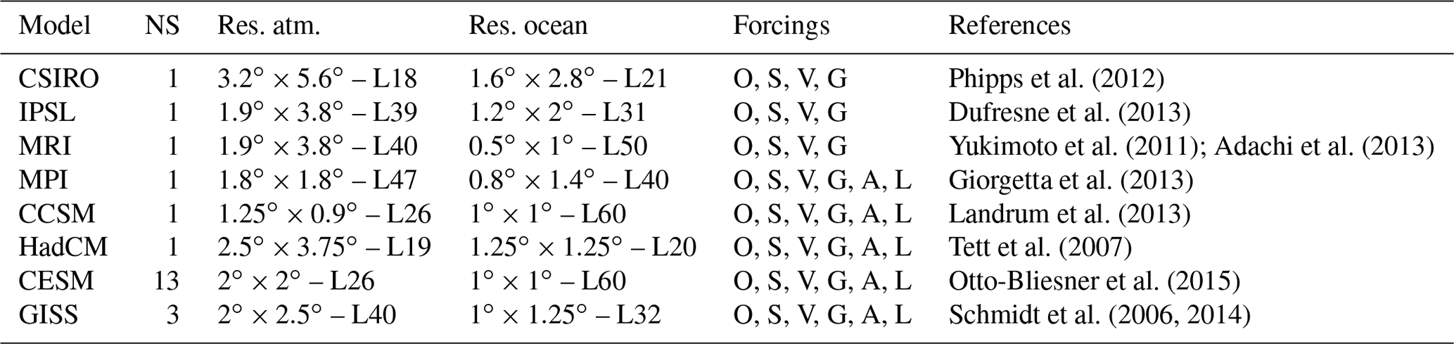
Even if ensembles with individual forcing factors and with reduced sets of forcings are available for some particular models, only simulations with the most complete set of external forcings that were available for each model have been considered herein. As shown in Table 1, all the analyzed simulations include solar variability, volcanic eruptions, greenhouse gases, and orbital changes as external forcings, while most of them also include land use and cover changes and anthropogenic aerosols. The reconstructions of forcings considered for each simulation can be found in Masson-Delmotte et al. (2013) for the CMIP5/PMIP3 simulations and in Otto-Bliesner et al. (2015) for the CESM-LME simulations. The forcing factors are similar in all the simulations, which are based on the guidelines for CMIP5/PMIP3 (Schmidt et al., 2011, 2012). The greenhouse gases are mainly obtained from MacFarling-Meure et al. (2006), the orbital changes from Berger (1978), the volcanic forcing from Gao et al. (2008) and Crowley and Unterman (2013), the solar variability from Vieira et al. (2011), Wang et al. (2005), and Steinhilber et al. (2009), the land use from Pongratz et al. (2008), and the aerosols from Lamarque et al. (2010).

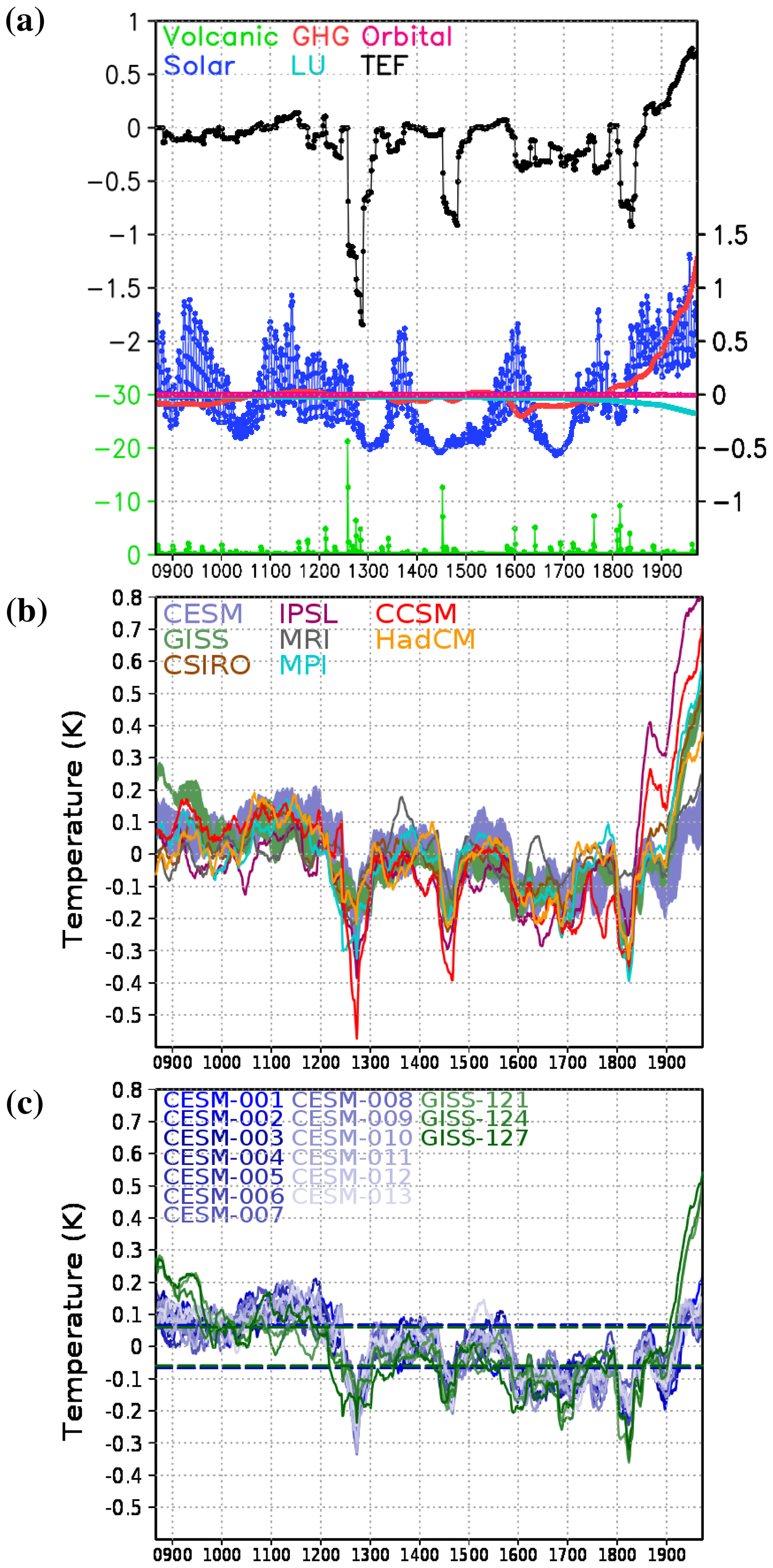
Figure 1 (a) External forcing factors (in W m⁻²) considered in the CESM-LME simulations, including greenhouse gases (GHGs), volcanic, solar, land use and cover (LU), and orbital forcing. The CESM-LME is selected as an example since it uses standard CMIP5/PMIP3 forcing specifications (Schmidt et al., 2011, 2012). The forcing related to greenhouse gases is obtained by aggregating the contributions of CO₂, CH₄, and N₂O. Volcanic forcing is represented with a different scale (in green). An evaluation of the total external forcing (TEF) following Fernández-Donado et al. (2013) is also included. (b) Global average of temperature in the ensemble of simulations. For CESM and GISS, the range of minimum and maximum values in the subensemble at each time step is shown instead of individual model simulations. All temperature and TEF series have been 31-year low-pass filtered with a centered moving average. (c) Individual simulations in CESM and GISS subensembles. Dashed blue (CESM) and green (GISS) lines represent the range ($\stackrel{\mathrm{‾}}{x}\pm \mathrm{2}$ SD) of the differences between each 31-year low-pass filtered member and the ensemble mean with $\stackrel{\mathrm{‾}}{x}$ being the mean of the residual and SD the standard deviation.

Figure 1 plots the forcing factors considered in the CESM-LME simulations as an example of the LM forcings. The figure also shows an estimation of the total external forcing (TEF) obtained following Fernández-Donado et al. (2013) by aggregating the contributions of solar activity, orbital changes, volcanic activity, greenhouse gases (GHGs) including CO₂, CH₄, and N₂O, land use change, and anthropogenic sulfate aerosols, which are converted into radiative forcing units and filtered with a moving average of 31 years. Even if it presents some limitations in the conversion of volcanic forcing and the contribution of aerosols (Fernández-Donado et al., 2013), the TEF allows analyses of the long-term evolution of the overall incoming energy with long intervals of higher (MCA and industrial era) and lower (LIA) forcing, as well as multidecadal to centennial changes produced by the combination of solar and volcanic activity.

The response to external forcing of temperature and a number of variables representative of atmospheric circulation and hydroclimate conditions is analyzed, namely sea level pressure (SLP), zonal wind (U), precipitation (P), soil moisture (SM), precipitation minus evaporation (P–E), and the Palmer Drought Severity Index (PDSI; Palmer, 1965), with the potential evapotranspiration calculated using Thornthwaite's method (Thornthwaite, 1948). While this formulation of PDSI has been shown to be problematic for soil moisture assessments during projections of the 21st century, differences between various formulations of PDSI have been shown to be minimal over the LM interval even when the 20th century is included (Smerdon et al., 2015). Characterizing the hydrological state of the soil is challenging because different general circulation models (GCMs) incorporate different land models and soil moisture physics. This work is focused therefore on precipitation, on P–E as a descriptor of general surface hydrological interactions, and on soil moisture and PDSI as descriptors of soil moisture content. PDSI is incorporated to employ a homogeneous description of soil moisture content across models because it is calculated from atmospheric variables and assumes the same soil parameters across all of the models. It has been defined following the self-calibrating PDSI (scPDSI; Wells et al., 2004). All simulations have been interpolated to a common $\mathrm{6}{}^{\circ }\times \mathrm{6}{}^{\circ }$ grid resolution, the coarsest among the analyzed simulations.

At interannual scales, some events of external forcing such as volcanic eruptions are able to explain considerable changes in the analyzed variables (Fischer et al., 2007). To assess the impact of such events on the climate, we use a superposed epoch analysis (SEA) by defining a composite with the main volcanic eruptions within the LM and computing for this composite the global average of the variables previously mentioned for the 5 years before and 10 years after the events, which are selected following the procedure in Masson-Delmotte et al. (2013). For simulations from CESM-LME and CCSM, which use the reconstruction from Gao et al. (2008) as volcanic forcing, the years of the composite have been selected based on the minima of forcing from this reconstruction: 1452, 1584, 1600, 1641, 1673, 1693, 1719, 1762, 1815, 1883, 1963, and 1990. For the other simulations, the reconstruction from Crowley and Unterman (2013) has been considered: 1442, 1456, 1600, 1641, 1674, 1696, 1816, 1835, 1884, 1903, 1983, and 1992. The significance of the changes in the variables evaluated within the SEA has been calculated using a bootstrap method. In total, 2200 sets of 12 years (100 for each simulation) have been randomly taken from the whole analyzed period, excluding the years of volcanic eruptions and the 10 years after them, to generate a distribution of averages for each variable. The significance of the averages computed after the 12 volcanic eruptions are then determined using the 5 and 95 confidence limits from the bootstrap distribution.

We use principal component (PC) analyses to describe the spatiotemporal response of variables at multidecadal to centennial timescales. The analysis has been applied to data which have been low-pass filtered with a moving average of 31 years in order to emphasize the response to external forcing versus internal variability (Fernández-Donado et al., 2013). We concatenate all of the low-pass filtered simulations to determine the empirical orthogonal functions (EOFs) across all of the models. The PCs are later obtained by projecting each individual simulation on the EOF, and, to assess the agreement among different simulations, the correlation coefficients between PCs from each simulation have been computed. This method allows us to obtain the modes of variability that explain a greater percentage of variance when considering the whole ensemble because the covariability with external forcing is expected to show common features across models and simulations.

The results presented herein have been confirmed for consistency with an individual analysis of each model simulation. The single experiment EOFs bear only regional differences that do not contradict the results obtained with the combined analyses, with spatial correlations with the multi-model EOFs reaching 0.9 for some simulations and 0.7 for most of them. The analyses have been repeated but by weighting the simulations so that each model would have the same influence, and the results are consistent (not shown). The concatenation of some relatively large subensembles (GISS and CESM-LME) may bias the results to these models, but these additional analyses confirm that this is not the case. As an advantage, the concatenation of all simulations allows us to define EOFs that are valid for all models. Additionally, the incorporation of two subensembles allows for insights about the effects of internal variability since the GISS and CESM ensembles incorporate identical boundary conditions and different initial conditions for each simulation.

To identify which modes from those obtained in the PC analyses are capable of showing responses to external forcing, the correlation coefficients between their associated PC time series and the first PC of temperature have been computed, and only those showing the highest correlations have been analyzed in detail. The use of the first mode of temperature instead of the time series of external forcing factors removes the dependency on the particular reconstructions used by each model simulation. To confirm that the first mode of temperature is linked to the external forcing for the analyzed simulations, the correlation coefficient between the PC time series associated with this mode and the respective time series of the TEF used for each specific model have been computed. The significance of these correlations has been assessed with Student's t test for the correlation coefficient using an effective number of degrees of freedom that considers the window of the moving average applied to the input data.

For a more detailed analysis of the long-term changes during the transition from the MCA to LIA, composites for the MCA and LIA have been defined from the ensemble average of each variable. The temporal phasing of these periods is regionally dependent and relies on the specific reconstruction or model (Neukom et al., 2014, 2019). For these analyses, the temporal intervals of these periods have been adopted from Masson-Delmotte et al. (2013), with the MCA ranging from 950 to 1250 CE and the LIA from 1450 to 1850 CE, although these time frames may not be regionally optimal. Composite maps of the differences between these two periods are derived for temperature, SLP, zonal wind, precipitation, soil moisture, P–E, and scPDSI. The significance of these MCA–LIA differences is assessed by performing Student's t test for the difference of averages between the MCA and LIA for each grid point.

To better analyze the changes in the extratropical zonal circulation, the NAO, NAM, and SAM indices have been computed. The NAO index was obtained (Stephenson et al., 2006) with the difference of boreal winter (December, January, and February; DJF) SLP average for 20 to 55^∘ N, 90^∘ W to 60^∘ E and 55 to 90^∘ N, 90^∘ W to 60^∘ E. The NAM index was calculated (Li and Wang, 2003) as the difference between the DJF zonal mean SLP at 35 and 65^∘ N, and the SAM index was calculated from the difference between the zonal mean of annual SLP at 40 and 65^∘ S (Gong and Wang, 1999). The NAO, NAM, and SAM indices have been obtained for each simulation from Table 1. The average of all the simulations was subsequently computed to determine the percentage of years with positive phases for successive intervals of 50 years. The change in the percentage of positive phases from the MCA to LIA was in turn assessed and the significance of the changes evaluated using Student's t test.

3 Results

3.1 Temperature

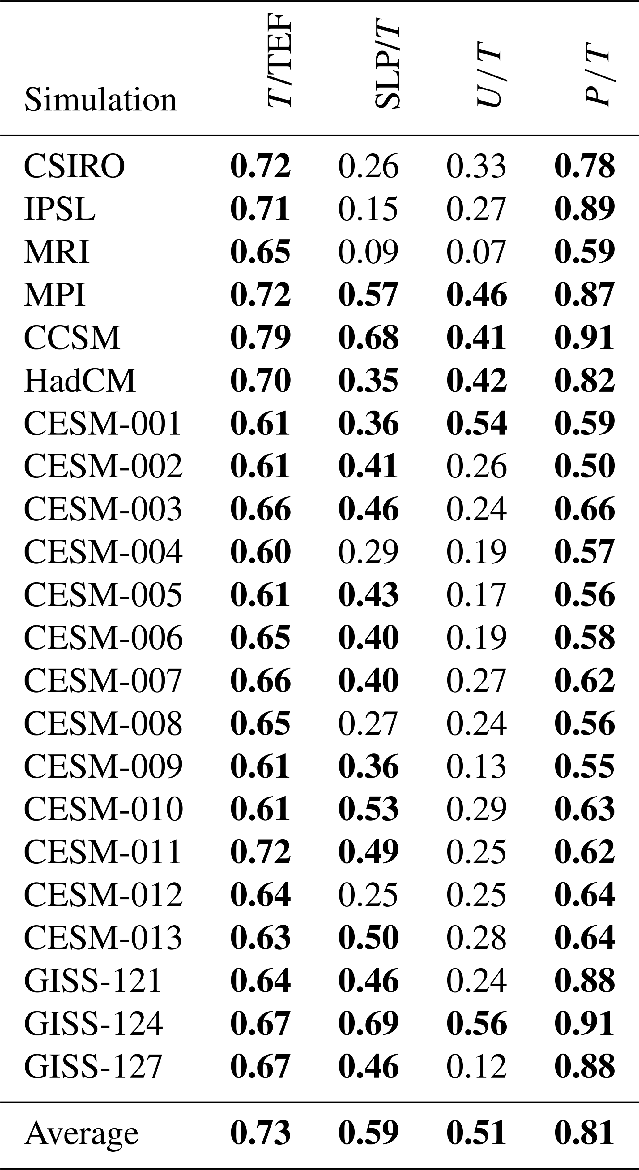
Figure 1 shows global temperature averages for all the ensemble members listed in Table 1. As reported by Fernández-Donado et al. (2013) in the case of the pre-PMIP3 LM experiments, there is a quasi-linear response of temperatures to changes in external forcing, with the major warmings occurring in periods with high solar activity and rise in GHGs and with coolings occurring in response to lower solar forcing and increased volcanic activity. For the 20th century, all the analyzed simulations consistently show a warming, but trends strongly differ among simulations due to the different climate sensitivities of each model (Vial et al., 2013) and the considered forcings (see discussion in Fernández-Donado et al., 2013). Simulations from IPSL, CCSM, and GISS show a very strong trend, while simulations from CESM show a significant but smaller 20th century temperature increase. The results for the GISS and CESM subensembles are shown in Fig. 1b by plotting the minimum–maximum spread of all subensemble members, while Fig. 1c shows, for the sake of clarity, the behavior of each subensemble member. These subensembles demonstrate that internal variability generates differences across simulations that are smaller than structural differences in model formulation across models. Figure 1c shows the range (dashed lines) of the residuals resulting from subtracting the ensemble mean from each ensemble member simulation. Since the average of all ensemble members cancels out uncorrelated contributions of internal variability, the resulting ensemble mean constitutes a smoothed estimation of the forced response, and the residuals of subtracting the ensemble mean from each ensemble member are an estimation of internal variability above 31-year timescales (Crowley, 2000; PAGES2k-PMIP3 group, 2015). Both the CESM and GISS ensembles in Fig. 1c show pre- and post-1850 low-frequency changes greater than the estimated changes of internal variability. Changes in the ensemble associated with external forcing are therefore in general more relevant than those of internal variability above 31-year timescales. A similar behavior is found when performing a PC analysis of the simulated temperatures, as shown in Fig. 2, with the first temperature EOF and PC estimates obtained from the simulations listed in Table 1. Agreement between the different simulations is very good, all of them showing the same long-term trends described for Fig. 1. Figure 2 also shows the correlation among the estimated PCs of different simulations. Note that most of the analyzed simulations show correlations higher than 0.5 and that for simulations of the same model the correlations reach values around 0.9 both when analyzing the whole period and when considering only the preindustrial era. This indicates that even if the EOF has been obtained with a combined analysis, it is also representative of the individual simulations. Additionally, the use of large sets of simulations for some of the models, and in particular the use of the 13 CESM-LME simulations, does not significantly bias the results because the correlation ranges for models with individual simulations are as large as for the others. The variance of temperature that the first PC accounts for in the ensemble is greater than 50 % across all of the models, significantly greater than the variance explained by the remaining modes (Fig. 3). To evaluate whether this first mode is related to the forcing, the correlations of the PC of each simulation with the TEF (Fig. 1a) have been included in Table 2. All the correlations are significant and range between 0.61 and 0.79. The first PC of temperature is therefore mainly attributed to external forcing, and for this reason dynamics and hydroclimate variables are compared in the following sections against this mode to explore their forced responses.

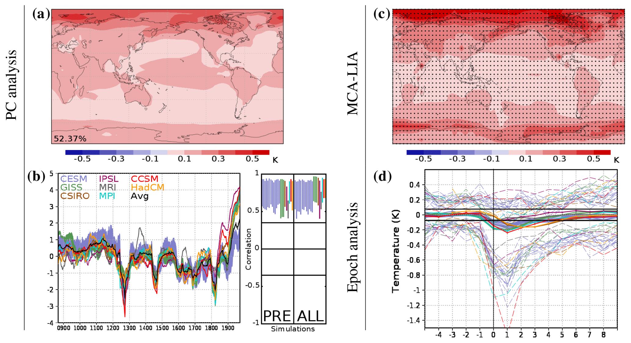
Figure 2 Analysis of temperature for the ensemble of simulations included in Table 1. (a) First EOF and (b) first PC time series for each simulation, as well as the average PC of all the simulations (black line). The percentage of explained variance is shown within the EOF map. The range of correlations between the PC of each simulation and those of other simulations is also included on the right of the plotted PCs both for the whole period (ALL) and for the preindustrial era (PRE). For these correlations, the significance level (p<0.05) accounting for autocorrelation is shown with a black line. (c) Map of temperature differences between MCA and LIA. Dots indicate locations where the differences are significant (p<0.05). (d) Composite average (solid lines) and maximum and minimum (dashed lines) global temperature anomalies in the 5 years before and 10 years after the 12 main volcanic eruptions of the LM. The vertical line indicates the year of the volcanic event. The horizontal black lines show the significance level of the average (p<0.10) based on the distribution of averages of 12 years generated with 2200 sets randomly taken from the whole period excluding the years of the 12 main volcanic eruptions and the 10 years after them.

Figure 3 Percentage of variance explained by the first eight modes obtained with the multi-model EOF analysis of temperature, SLP, zonal and meridional wind, precipitation, soil moisture, P–E, and scPDSI.

Table 2 Correlations between the first PC of surface temperature of each model simulation and TEF (Fig. 1a) and correlations for different simulations of the PC linked to the forcing for sea level pressure, zonal wind, and precipitation (first PC of SLP and zonal wind and second PC of precipitation) with the first PC of surface temperature. Correlations of the average PC time series are also included. Significant correlations (p<0.05) accounting for autocorrelations are shown in bold.

Regarding the spatial pattern of the EOF, values are higher over continental regions and smaller over oceans. For high latitudes, higher values are obtained over ice-covered areas, which is consistent with the polar amplification response in climate change scenarios (Bindoff et al., 2013). For all regions, the first EOF shows positive loadings, meaning that situations of higher forcing correspond to higher temperatures for the whole planet and vice versa. This pattern has been discussed in Zorita et al. (2005) and Fernández-Donado et al. (2013), and similarities can also be observed of the differences between the MCA and LIA (Fig. 2c). The transition from MCA to LIA in most regions leads to a decrease in simulated temperatures, which is consistent with the negative external forcing anomalies applied in the simulations. The MCA–LIA pattern does not emphasize the tropics as much as the EOF pattern, indicating that the low-frequency variability changes in that area are minor and that the higher tropical loadings in Fig. 2a stem from covariability at higher frequencies. Also note that area weighting has been applied to the EOF calculations, increasing the contribution of the tropical areas in these analyses.

At shorter timescales, the influence of external forcing is also evident. Figure 2d shows the average, maximum, and minimum temperatures for the composite with the 5 years before and 10 years after the 12 main volcanic eruptions of the LM. Note that global temperature significantly decreases after these events and that their influence lasts several years until it totally disappears. Important differences exist among models in the response to volcanic eruptions. Some simulations, such as those from GISS, MPI, CESM, and CCSM, show a drastic cooling after volcanic events that is mostly recovered after four years. However, simulations from HadCM and CSIRO show a moderate cooling that lasts for a longer period.

3.2 Atmospheric dynamics

To evaluate the possible influence of external forcing on global atmospheric dynamics, the same analyses performed for temperatures have been applied to SLP. Figure 4 shows results for the different timescales. The long-term behavior of the first PC of pressure is comparable to that of the first PC of temperature. For the case of pressure, the average PC (black line in Fig. 4b) tends to show higher values during the MCA, lower during the LIA, and a significant increase during the last century. The similarity of the first PC of SLP with that of temperature can be quantified through the correlation coefficient values (Table 2), which are significant for 73 % of the simulations in the ensemble and above 0.5 for 23 % of them. The average PC correlates with a value of 0.59 (Table 2) with the corresponding PC of temperature (black line in Fig. 2b). This suggests some response to external forcing in the SLP field. The first mode accounts for only 15 % of the variance in the pressure, showing an eigenvalue spectra flatter than the one of temperatures (Fig. 3). This indicates that even if there is a response to external forcing, internal variability is more relevant than in the case of temperature. Additionally, the correlations among PCs of different simulations are in general not significant over the preindustrial period (Fig. 4b). When the whole period is considered, more significant correlations are obtained.

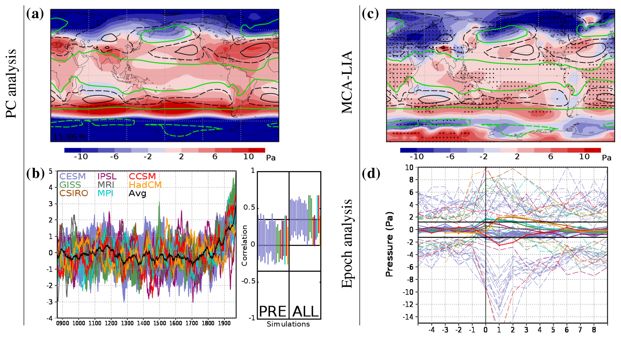
Figure 4 Analysis of SLP for the ensemble of simulations included in Table 1. (a) First EOF and (b) first PC time series for each simulation, as well as the average PC of all the simulations (black line). The percentage of explained variance is shown within the EOF map. The range of correlations between the PC of each simulation and those of other simulations is also included on the right of the plotted PCs both for the whole period (ALL) and for the preindustrial era (PRE). For these correlations, the significance level (p<0.05) accounting for autocorrelation is shown with a black line. (c) Map of SLP differences between MCA and LIA. Dots indicate locations where the differences are significant (p<0.05). Contours with climatological SLP of 986 hPa (dashed green), 1012 hPa (solid green), 1016 hPa (dashed black), and 1020 hPa (solid black) are included in the EOF and MCA–LIA maps. (d) Composite average (solid lines) and maximum and minimum (dashed lines) global SLP anomalies in the 5 years before and 10 years after the 12 main volcanic eruptions of the LM. The vertical line indicates the year of the volcanic event. The horizontal black lines show the significance level of the average (p<0.10) based on the distribution of averages of 12 years generated with 2200 sets randomly taken from the whole period excluding the years of the 12 main volcanic eruptions and the 10 years after them.

The EOF indicates that the first mode is mainly extratropical (Fig. 4a). In the SH, there is an increase in pressure (positive loadings) around 40^∘ S and a decrease (negative loadings) around 80^∘ S during the MCA (higher PC values) and conversely during the LIA. This spatial pattern, with positive loadings over the maxima of climatological SLP (black contours of Fig. 4a) and negative loadings over the minima (green contours of Fig. 4a), contributes to the positive phase of the mode to intensify gradients between subtropical and subpolar regions. This reinforces zonal circulation and contributes to more positive phases of the SAM (Jones et al., 2009; Fogt et al., 2009), as shown in Fig. 5. Regarding the NH, the pattern of pressure associated with the first mode is not as zonal as in the SH mostly because of the interaction with the continents. Overall, higher positive (negative) loadings are distributed over subtropical (polar) regions contributing to an increase (decrease) in the zonal flow during the MCA and industrial period due to the slightly higher values of the PC, which are also consistent with NAM (Thompson and Wallace, 2001) enhancement.

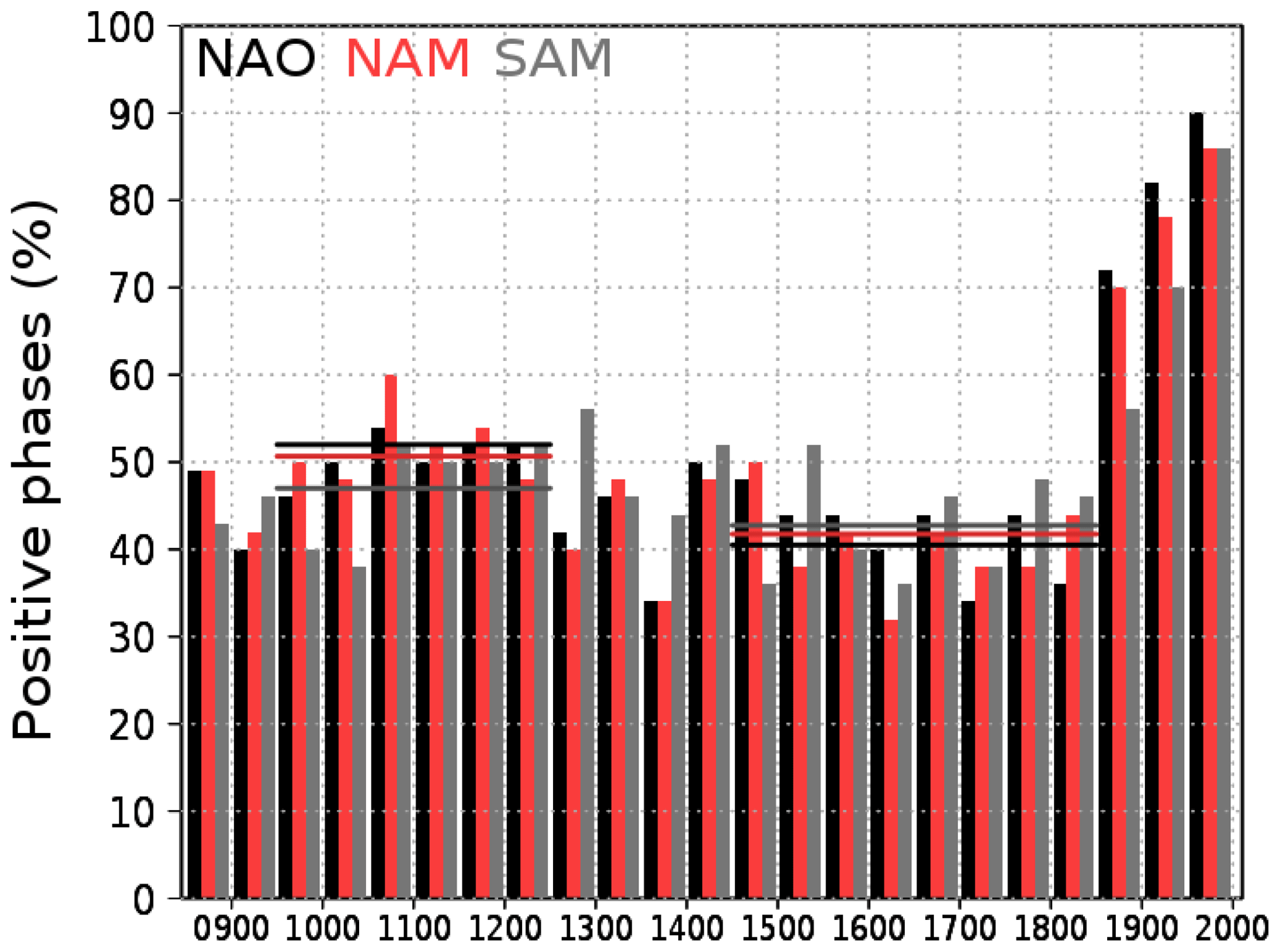
Figure 5 Percentage of years with positive NAO, NAM, and SAM indices for each interval of 50 years. Horizontal lines show the total percentage for the MCA and the LIA. The differences between MCA and LIA are significant with p<0.05 for NAO and NAM and with p<0.15 for SAM.

As in the leading EOF, the spatial pattern of the MCA–LIA differences (Fig. 4c) also emphasizes the latitudinal gradients. Even if the exact boundaries between areas with positive and negative MCA–LIA differences do not fully match the zonal features of the first EOF loadings, the ensemble average shows the largest differences over the subpolar and subtropical regions, which contribute to the enhancement of the zonal flow in the MCA and to the weakening of it during the LIA. This pattern is associated with an intensification (MCA) and weakening (LIA) of the SAM, NAM, and NAO, as shown in Fig. 5. The figure shows the percentage of years with positive NAO, NAM, and SAM indices for successive intervals of 50 years. Consistent with the spatial patterns and temporal evolutions shown in the PC analysis, a tendency toward more positive phases of the NAO, NAM, and SAM is observed during the MCA and industrial periods.

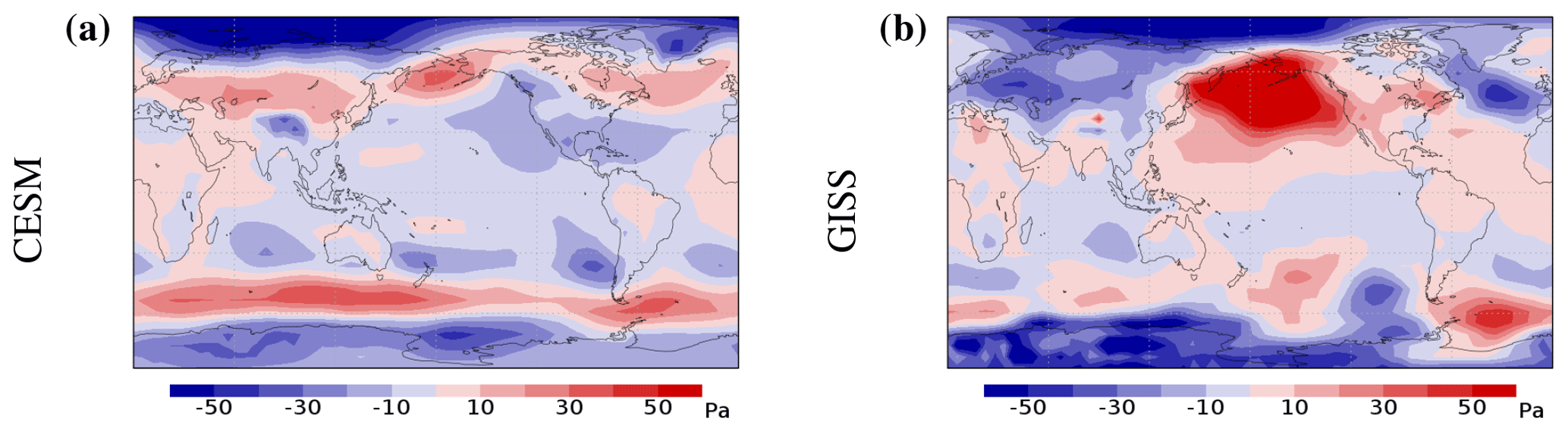
Figure 6 Maps of SLP anomalies for the 10 years after the 12 main volcanic eruptions of the LM. (a) Average of simulations from the CESM subensemble. (b) Average of simulations from the GISS subensemble.

Due to the large range of internal variability, the short-term response to volcanic forcing is not so evident in the PC of SLP as it is in the case of temperature. However, a low-frequency signal is observed in the mean PC series (Fig. 4b) for which high frequencies are canceled out. If the largest volcanic events are considered, a clearer response emerges. Figure 4d shows the global average of SLP for the composites for the 5 years before and 10 years after the main volcanic eruptions of the LM. Note that the global average of SLP shows significant changes triggered by volcanic activity. The sign and magnitude of the global net changes strongly depend on the model, but there is good agreement among simulations of the same model. For instance, simulations from GISS show an increase in pressure after volcanic events, while simulations from CESM-LME consistently show a decrease. This difference in the global average of pressure is not related to an opposite response in different models but to the distribution of areas with positive and negative loadings in the mode of variability associated with the forcing. As shown in Fig. 6, simulations from CESM show a greater number of areas with negative anomalies during periods with volcanic events, while simulations from GISS tend to show more areas with positive anomalies. In spite of the differences in the global balance of regional positive and negative anomalies between GISS and CESM-LME simulations, both produce a global weakening in zonal circulation during volcanic eruptions.

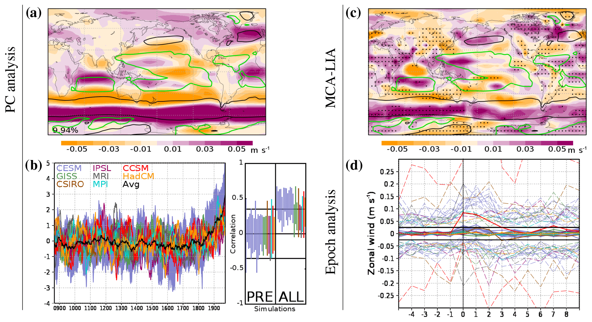
Figure 7 Analysis of zonal wind for the ensemble of simulations included in Table 1. (a) First EOF and (b) first PC time series for each simulation, as well as the average PC of all the simulations (black line). The percentage of explained variance is shown within the EOF map. The range of correlations between the PC of each simulation and those of other simulations is also included on the right of the plotted PCs both for the whole period (ALL) and for the preindustrial era (PRE). For these correlations, the significance level (p<0.05) accounting for autocorrelation is shown with a black line. (c) Map of zonal wind differences between MCA and LIA. Dots indicate locations where the differences are significant (p<0.05). Contours with climatological wind of −6 m s⁻¹ (east winds; green) and 6 m s⁻¹ (west winds; black) are included in the EOF and MCA–LIA maps. (d) Composite average (solid lines) and maximum and minimum (dashed lines) global zonal wind anomalies in the 5 years before and 10 years after the 12 main volcanic eruptions of the LM. The vertical line indicates the year of the volcanic event. The horizontal black lines show the significance level of the average (p<0.10) based on the distribution of averages of 12 years generated with 2200 sets randomly taken from the whole period excluding the years of the 12 main volcanic eruptions and the 10 years after them.

Some studies have shown that elevated forcings during the 20th century may be linked to a displacement of the ITCZ and an expansion of Hadley cells (Sachs et al., 2009; Lu et al., 2007; Seager et al., 2007). This can be described in terms of wind velocity, in which the ITCZ is defined by the location of the trade winds and the extension of Hadley cells is marked by the position of the westerlies (Frierson et al., 2007). Thus, the previous analysis is also performed for the zonal wind (Fig. 7). In this case, the first mode accounts for 10 % of the total variance, a smaller percentage than for the case of temperature and SLP. The average PC of zonal wind shows a correlation of 0.51 with the average PC of temperature and 0.96 with that of SLP, indicating a response to the external forcing consistent with the one observed in temperature and SLP. However, the correlation with the PC of temperature for the individual simulations is in general small, indicating a greater impact of internal variability. As shown in Table 2, only five simulations show significant correlations, and only two of them are higher than 0.5. The agreement among different simulations can also be assessed through the correlations among their respective PCs, which are in general not significant when the preindustrial period is considered and are only significant for certain simulations when they are based on the whole period (Fig. 7b). The correlation between the corresponding PC time series of zonal wind and that of SLP for each simulation is always above 0.7.

Thus, the distribution of zonal wind in the first EOF is consistent with the distribution of pressures previously shown. In the positive phase of the mode, negative (positive) loadings tend to distribute over the easterlies (westerlies) and over their high-latitude side, thus increasing latitudinal gradients and contributing to a polar displacement of the wind system; trade winds are enhanced towards higher latitudes in the Atlantic and eastern Pacific. This is consistent with an expansion of the Hadley cell and the higher intertropical loadings and MCA–LIA anomalies in Fig. 4. The same behavior can be observed in the composites for the MCA and LIA, in which a poleward displacement of the westerlies is present during the simulated MCA relative to the LIA. However, the spatial pattern of the difference between the MCA and LIA differs for some regions relative to the one obtained from the EOF. For example, the differences between MCA and LIA indicate a reduction of zonal wind in the Mediterranean basin and an increase over Japan in the transition from MCA to LIA (Fig. 7c), while the loading in the EOF for these particular areas (Fig. 7a) is negative and positive, respectively.

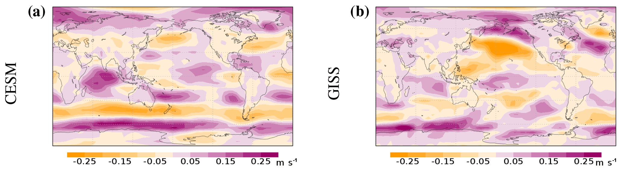
Figure 8 Maps of zonal wind anomalies for the 10 years after the 12 main volcanic eruptions of the LM. (a) Average of simulations from the CESM subensemble. (b) Average of simulations from the GISS subensemble.

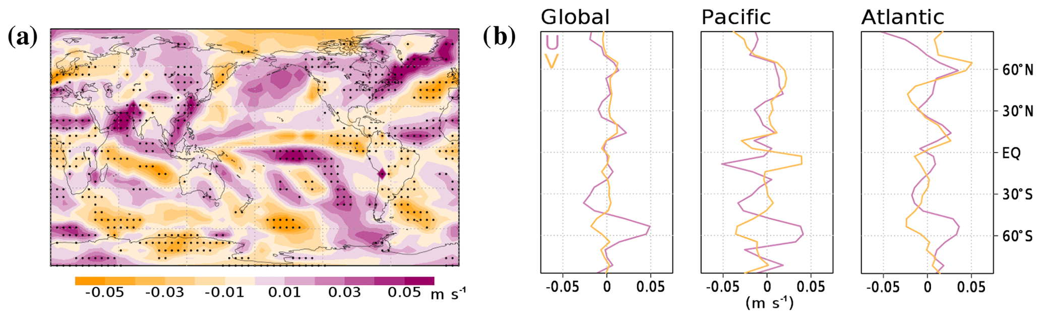
Figure 9 (a) Map of meridional wind differences between MCA and LIA. Dots indicate locations where the differences are significant (p<0.05). (b) Zonal mean of zonal wind (purple) and meridional wind (yellow) for the composite MCA–LIA for global, central Pacific (180–120^∘ W), and Atlantic (50–0^∘ W) basins.

In the short term, the behavior of zonal wind resembles that of SLP. In most simulations, the short-term noise associated with internal variability dominates over the peaks associated with volcanic eruptions, as can be observed in Fig. 7b. When composites of the main volcanic eruptions are defined (Fig. 7d), a clear influence of volcanic activity emerges. As for the case of pressures, the sign of the impact depends on the model mostly because of the different spatial distribution of areas with positive and negative anomalies. This can also be observed when comparing maps of zonal wind during volcanic events obtained with the CESM and GISS subensembles (Fig. 8). In spite of the differences in some areas like the northern and tropical Atlantic and Pacific basins, both subensembles tend to weaken the global zonal circulation. However, the simulations from CESM (GISS) show more areas with positive (negative) zonal winds, which translate into a larger (smaller) increase in the global average. These zonal changes are also evident in the behavior of the meridional wind component. Figure 9 shows the differences between MCA and LIA in terms of meridional wind, as well as the zonal mean of these differences for zonal and meridional components for both global and regional Pacific (180–120^∘ W) and Atlantic (50–0^∘ W) basins (Fig. 9b). During the simulated MCA, changes in zonal and meridional winds took place with antiphase relationships that strengthened the zonal circulation at middle and high latitudes (Fig. 9b) with increases in the NAO, NAM, and SAM (Fig. 5), while within the intertropical regions the trade winds and convergence were intensified (Figs. 7c and 9). The opposite holds for the LIA.

3.3 Hydroclimate

For the case of precipitation, Figs. 10 and. 11 show the EOF and PC series for the leading two modes. Both modes show cross-basin influences in the tropical regions that connect the Indian, Pacific, and Atlantic oceans. Precipitation loadings are suggestive of ENSO, Pacific Decadal Oscillation (PDO), and monsoon influences (Christensen et al., 2013), thus showing large-scale coordinated responses that can connect in-phase or out-of-phase intra- and intercontinental responses. Although the first PC shows large negative values during the volcanically active 13th century and some slight increase during the 20th century, it is the second PC that resembles the external forcing response. Furthermore, its EOF emphasizes the distribution of monsoon precipitation over the global monsoon domain within the intertropical region. In the extratropics, the EOF pattern (Fig. 11a) shows distributions of loadings that are consistent with changes in NH NAM and SH SAM circulation. The PC series (Fig. 11b) clearly shows the long-term trends associated with the external forcing with higher values during the MCA and 20th century and lower values during the LIA, as well as the short-term response to volcanic events, which is in agreement with the analysis of pressures (Fig. 4) and winds (Fig. 7).

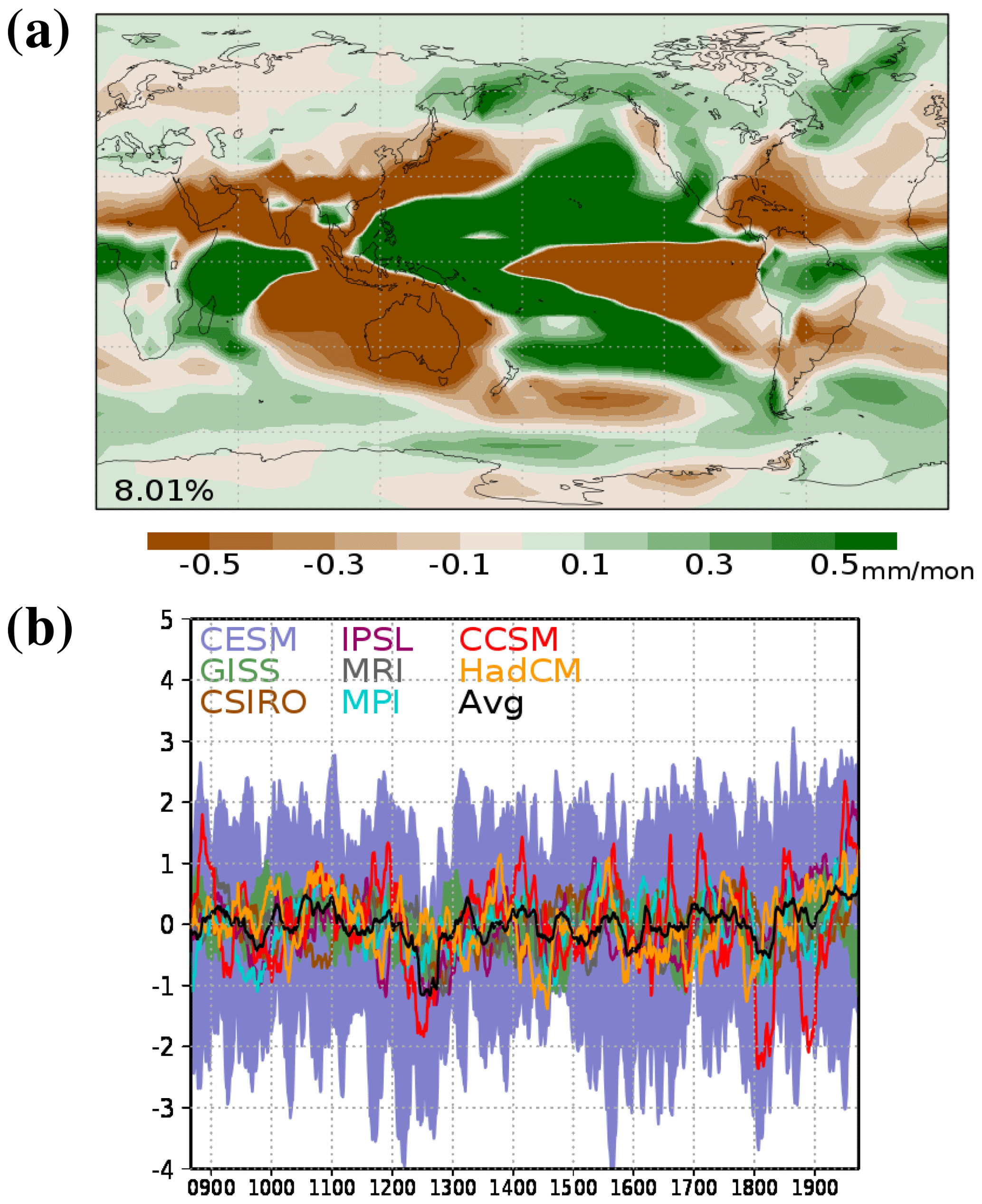
Figure 10 (a) First EOF of precipitation for the ensemble of simulations included in Table 1. The percentage of explained variance is shown within the EOF map. (b) PC time series for each simulation. The average of all the simulations is also included (black line).

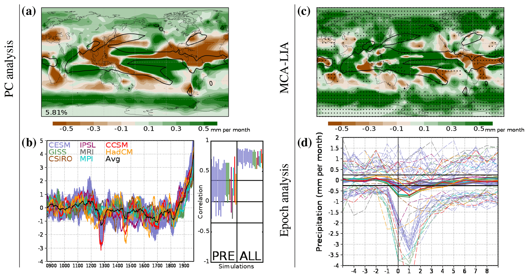
Figure 11 Analysis of precipitation for the ensemble of simulations included in Table 1. (a) Second EOF and (b) second PC time series for each simulation, as well as the average PC of all the simulations (black line). The percentage of explained variance is shown within the EOF map. The range of correlations between the PC of each simulation and those of other simulations is also included on the right of the plotted PCs both for the whole period (ALL) and for the preindustrial era (PRE). For these correlations, the significance level (p<0.05) accounting for autocorrelation is shown with a black line. (c)  Map of precipitation differences between MCA and LIA. Dots indicate locations where the differences are significant (p<0.05). Contours with climatological precipitation of 120 mm per month are included in black in the EOF and MCA–LIA maps. (d) Composite average (solid lines) and maximum and minimum (dashed lines) global precipitation anomalies in the 5 years before and 10 years after the 12 main volcanic eruptions of the LM. The vertical line indicates the year of the volcanic event. The horizontal black lines show the significance level of the average (p<0.10) based on the distribution of averages of 12 years generated with 2200 sets randomly taken from the whole period excluding the years of the 12 main volcanic eruptions and the 10 years after them.

There is good agreement between different models and different simulations with correlations being higher than 0.5 for simulations of different models and reaching 0.9 for different simulations of the same model (Fig. 11b; ALL). The correlation between the second mode of precipitation and the first mode of temperature (Table 2) is significant for all the analyzed simulations, ranging from 0.5 to 1 and being higher in the simulations from GISS, IPSL, and MPI and lower in the simulations from CESM and MRI. These values are higher than those obtained for pressure and winds. However, this mode accounts only for 5.8 % of the precipitation variance, a lower value than the one obtained for variables of dynamics. As seen in Fig. 3, the modes associated with internal variability acquire a greater relevance in the case of precipitation. This suggests that the potential detection of this signal in reconstructions would be difficult and, if possible, more likely at very local scales. The MCA–LIA differences (Fig. 11c) show some similarities with the EOF loadings in extratropical regions, indicating greater precipitation at northern latitudes in the MCA (Fig. 11c) or with increased forcing at all timescales above 31 years (Fig. 11a, b). Within the tropical regions, agreement is regionally complex, with MCA–LIA differences emphasizing low-frequency changes and EOF loadings including covariability at all timescales. Changes in dynamics described in Sect. 3.2 are consistent with the changes in precipitation. As for the case of dynamics, some zonal symmetry is observed in extratropical areas, suggesting that changes in the Northern and Southern Annular modes affect the distribution of precipitation in these regions. The highest variability occurs in intertropical areas over the regions with the greatest amount of annual rainfall, thus overlapping well with changes in the global monsoon domain and ITCZ convergence. MCA–LIA differences are regional in scope and show anomalies of different signs over the North and South American monsoon systems (NAMS, SAMS; Cerezo-Mota et al., 2011; Christensen et al., 2013), therefore without a clear response of NAMS and SAMS. This agrees with uncertainty in climate change projections over the NAMS, with CMIP5 models producing changes in precipitation that distribute around zero (Christensen et al., 2013). The same occurs over the Australian and Maritime Continent monsoon systems (AUSMC; Jourdain et al., 2013). Positive values are found over the East Asian and South Asian summer monsoon areas (EAS, SAS; May, 2011; Boo et al., 2011), which is in agreement with scenario simulations (Christensen et al., 2013). Even if changes are not significant over many of these regions due to the high variability of precipitation, they show a pattern of response to forcing in LM PMIP3 simulations consistent with that of scenario simulations; the consistency also extends to convergence zones. In the Atlantic and eastern Pacific north of the Equator (e.g., Xie et al., 2007), positive MCA–LIA differences suggest increases in mean precipitation during the MCA. Likewise, in the South Pacific Convergence Zone extending from the western Pacific southeastwards (e.g., Widlansky et al., 2011), positive differences also emerge, indicating increased rainfall during the MCA. Over South America, negative anomalies are found in the northwest of the climatological maxima (black contours in Fig. 11b) and positive anomalies in the southeast, depicting rainfall shifts in the South Atlantic Convergence Zone (Cavalcanti and Shimizu, 2012).

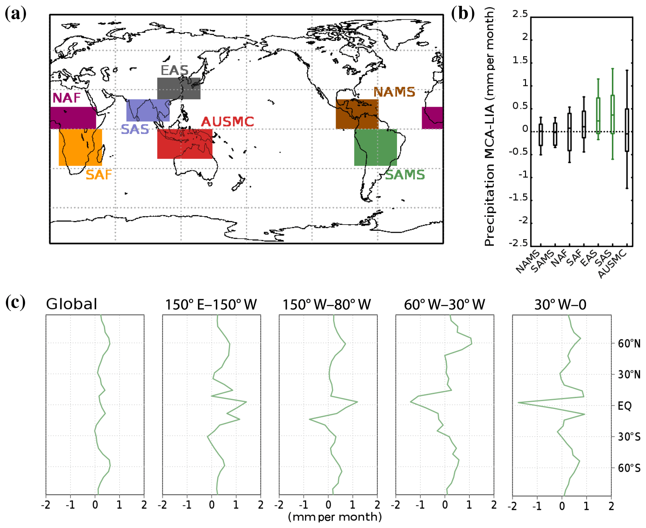
Figure 12 (a) Areas considered in the analysis of monsoon domains: North American monsoon system (NAMS), South American monsoon system (SAMS), the northern African (NAF), southern African (SAF), East Asian summer (EAS), South Asian summer (SAS) monsoons, and the Australian–Maritime continent (AUSMC). (b) Precipitation differences for MCA–LIA over the monsoon domains. Box and whisker plots show the 10th, 25th, 50th, 75th, and 90th percentiles of simulations included in Table 1. Domains with significant changes (p<0.05) have been highlighted in green. (c) Zonal mean of precipitation for the composite MCA–LIA for the whole globe and for bands of 150^∘ E–150^∘ W, 150–80^∘ W, 60–30^∘ W, and 30–0^∘ W.

To better analyze these changes, MCA–LIA precipitation differences are calculated for the monsoon domains in Fig. 12a. Changes in precipitation in the transition from the MCA to LIA (Fig. 12b) are small in NAMS and SAMS for all the analyzed simulations. Notice that over the NAMS and SAMS regions (Fig. 12a) both positive and negative MCA–LIA anomalies (Fig. 11c) are distributed, thus hampering a clear net response. The same happens over the northern African (NAF) and southern African (SAF) regions with an increase in model spread and SAF being biased towards increased precipitation during the MCA. Therefore, even if net regional responses are small due to the compensation of anomalies of different signs, subregional differences may be large. The greatest impact of the MCA-to-LIA transition in the monsoon systems appears over Asia, where EAS and SAS are significantly altered. Rainfall anomalies in EAS and SAS monsoon areas are larger during the MCA relative to the LIA. This pattern is consistently found in most of the simulations. For the AUSMC, some simulations show very positive differences while others are very negative, indicating that models all show important variations over this area but the magnitude and spatial distribution of these changes are strongly model-dependent. The global zonal mean of precipitation for the MCA–LIA (Fig. 12c) does not show important changes but only slightly larger values of precipitation anomalies during the MCA than during the LIA for most latitudes. However, if ranges of longitude over the Pacific and Atlantic basins are considered, relevant changes in the convergence areas are observed. The zonal mean for the range of 150^∘ E–150^∘ W shows higher precipitation rates during the MCA relative to the LIA in equatorial areas of the central and western Pacific. In the eastern Pacific (150–80^∘ W), precipitation is decreased (increased) north (south) of the Equator during the MCA-to-LIA transition, suggesting a southward displacement of the convergence zone. Ranges of 60–30 and 30–0^∘ W show that the convergence zone is also altered in the Atlantic basin with less intense precipitation around the Equator during the MCA than during the LIA.

Table 3 Correlations for different simulations of the PC linked to the forcing for soil moisture, P–E, and scPDSI (first PC of scPDSI and second PC of P–E and soil moisture) with the first PC of surface temperature and the second PC of precipitation. Correlations of the average PC time series are also included. Significant correlations (p<0.05) accounting for autocorrelations are shown in bold.

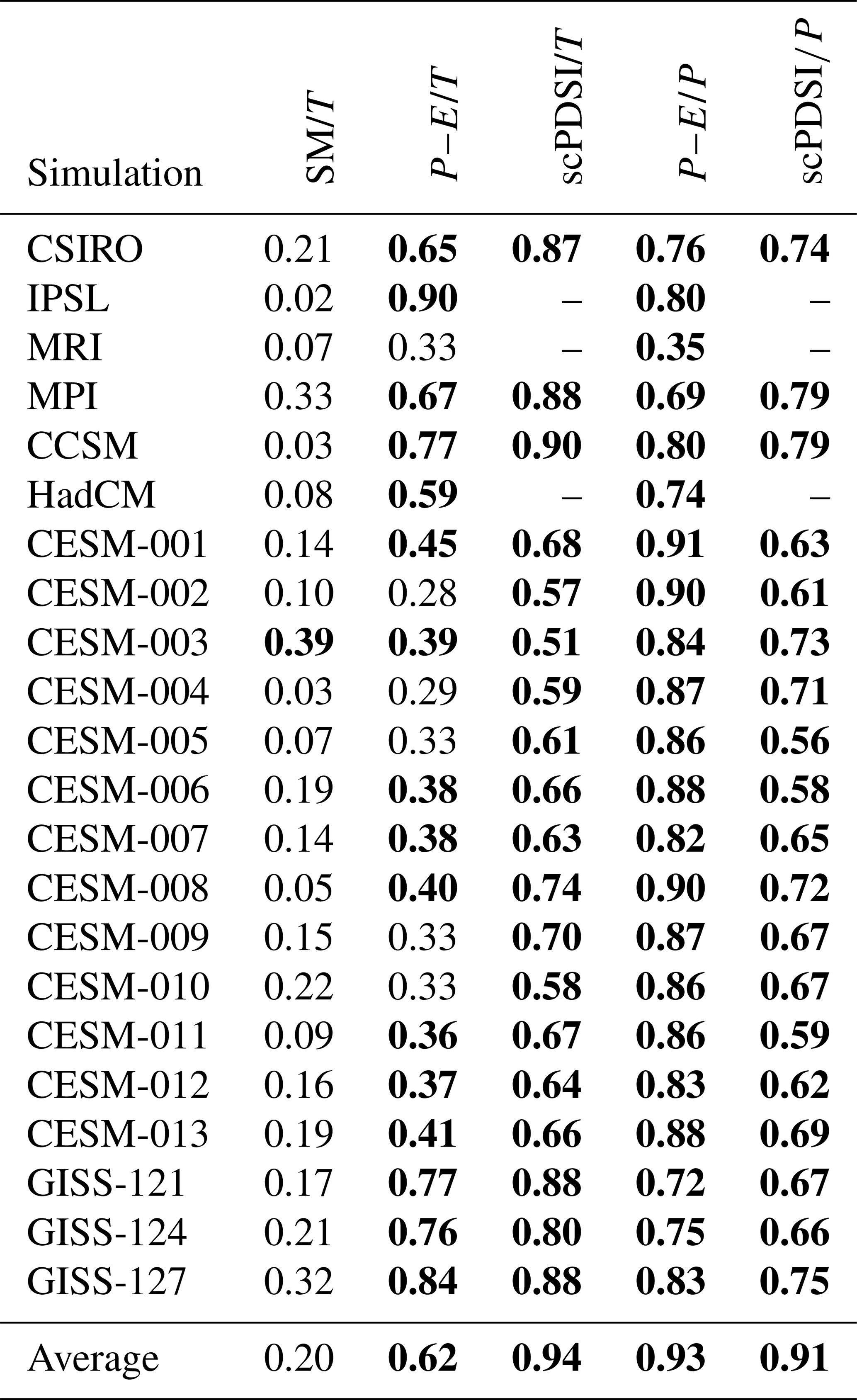
Figure 11d shows the global average of precipitation anomalies in the 5 years before and 10 years after the 12 main volcanic eruptions of the LM. A consistent decrease in global precipitation can be observed in all of the simulations after these volcanic events, being significant for most of them. The responses described for different timescales in Fig. 11 are consistent with changes in scenario simulations described in Christensen et al. (2013): increases in external forcing strengthen the hydrological cycle, enhancing zonal circulation in extratropical regions and increasing the global monsoon activity and equatorial convergence. This is found in the global average of precipitation after volcanic events and in the alteration of monsoons and latitudinal distribution obtained in the EOF, indicating a relevant response to external forcing in precipitation.

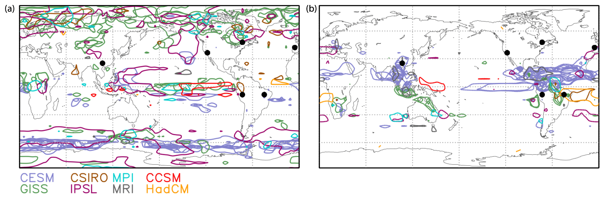
Figure 13 Regions showing high positive (a) or negative (b) correlation between precipitation and the mode of precipitation associated with the forcing for the ensemble of simulations included in Table 1. Contours of correlation equal to −0.6 and 0.6 are shown for each simulation. Dots indicate locations where the time series of Fig. 14 have been extracted.

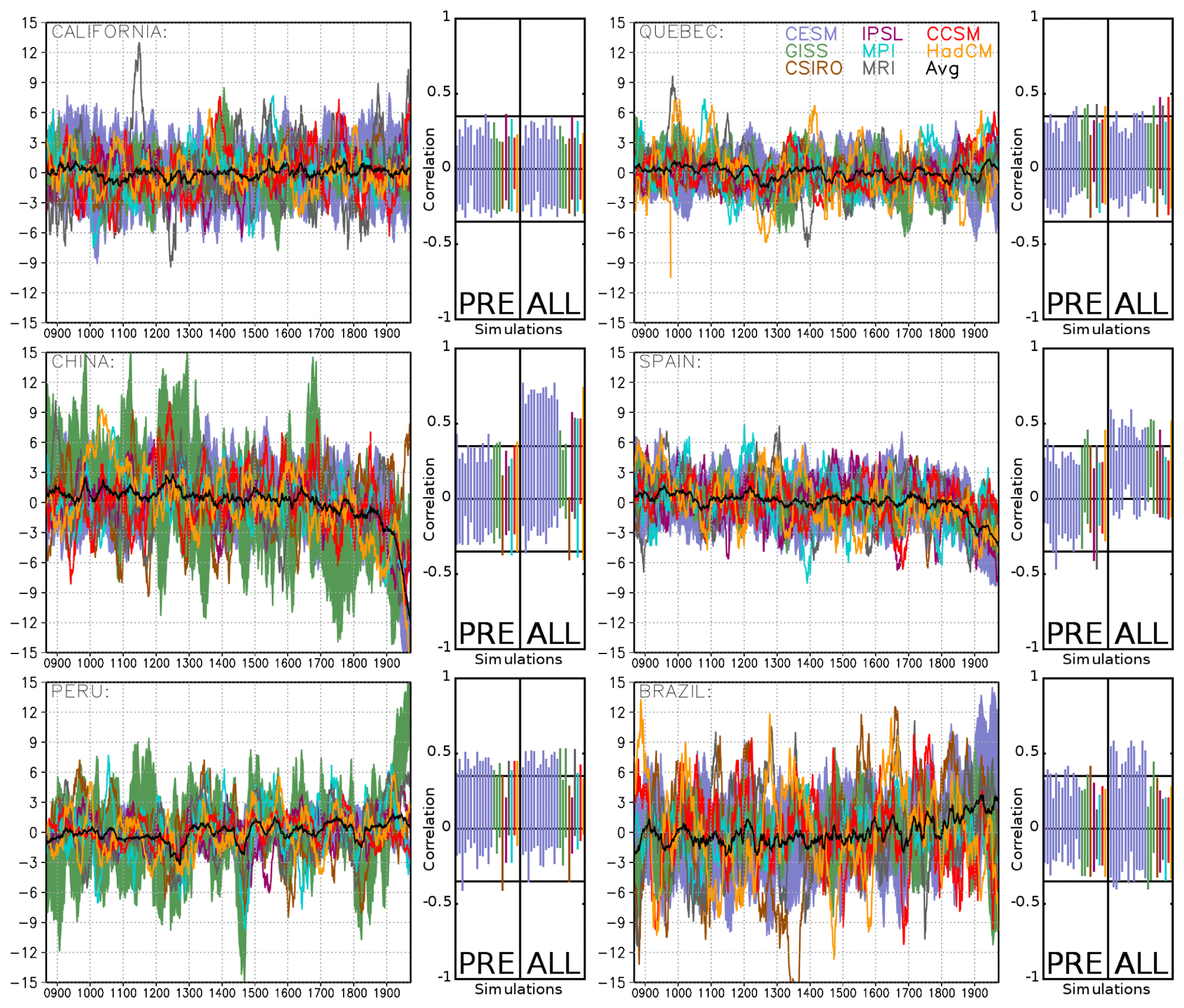
Figure 14 Time series of precipitation in millimeters per month for some particular case example locations. The range of correlations between the time series of each simulation and those of other simulations at those specific locations is also included both for the whole period (right; ALL) and for the preindustrial era (left; PRE). For these correlations, the significance level (p<0.05) accounting for autocorrelation is shown with a black line. All precipitation series have been 31-year low-pass filtered with a centered moving average.

Figure 13 explores the robustness of regional forcing influences on precipitation across models and simulations. It shows areas of high positive correlation (above 0.6, p<0.05; panel a) and regions of high negative correlation (below −0.6, p<0.05; panel b) between precipitation and the mode of precipitation associated with the forcing of the ensemble of model simulations. Most model simulations correlate with external forcing over the same large-scale regions: the high-latitude bands related to zonal NAM and SAM circulation changes (e.g., negative correlations in the south of Europe and positive in the north) and the intertropical regions related to monsoon domains and convergence. Some models show larger areas of sensitivity to forcing, while others present fewer regions where precipitation relates to the long-term changes in temperature produced by external forcing. For example, simulations from GISS show negative correlations in the north of Australia and the south of Africa that do not appear in simulations from CESM-LME. Despite most of the models showing positive correlations in the extratropical and tropical areas of the Pacific basin and negative correlations in tropical areas of the Atlantic basin and in southeastern Asia, the areas of high correlation are spatially constrained to regional and even local scales and may not overlap in different models or even in simulations of the same model. These regional differences are likely the sign of the important influence of internal variability. Correlations in high-latitude bands are all positive, while negative correlations arise mostly over the areas of monsoon activity in Africa, Asia, and America (Fig. 13b), as in the case of negative MCA–LIA anomalies discussed above. This view has implications for the detection of a potential response to global temperature and forcing changes in drought-sensitive proxy data (e.g., Ljungqvist et al., 2016) as the spatial dimension of the response can be quite limited particularly over land. Figure 14 shows examples of simulated precipitation at the grid-point level in cases that tend to show some correlation with forcing like Spain, China, and Peru (see grid-point locations highlighted with points in Fig. 13) and also at locations that tend to show limited connections to forcing within the ensemble: California, Quebec, and Brazil. At all these points, the different ranges of internal variability tend to be larger than the forcing signal. In some areas, the 20th century trends show precipitation increases, like in the selected Brazil and Peru sites, while in others there is no response (e.g., the California site) or precipitation tends to decrease (e.g., the selected sites in Spain and China). Inter-simulation correlations tend to increase during the 20th century for sites showing trends and remain insignificant for most inter-ensemble pairs in preindustrial times.

Similar results to those obtained for precipitation are obtained when analyzing other variables representative of the water content of the soil. P–E, scPDSI, and soil moisture in particular have been analyzed in this work. Even if these variables provide similar information, important differences exist between them. Because soil moisture takes into account the water balance in previous time steps, together with precipitation, evaporation, and temperature, its variations are typically smoother than those observed in atmospheric variables. Something similar happens with scPDSI, which similarly takes into account soil moisture conditions from the previous months. Due to the higher number of factors considered in the computation of soil moisture and the fact that this variable is fully integrated within the models, it is a preferred variable for assessing drought variability in the models. However, different GCMs and their respective soil models may provide different treatments of soil moisture, making it difficult to combine data from different models in a single analysis. For this reason, the use of indices, such as scPDSI, may provide more consistent comparisons across different models (e.g., Cook et al., 2014).

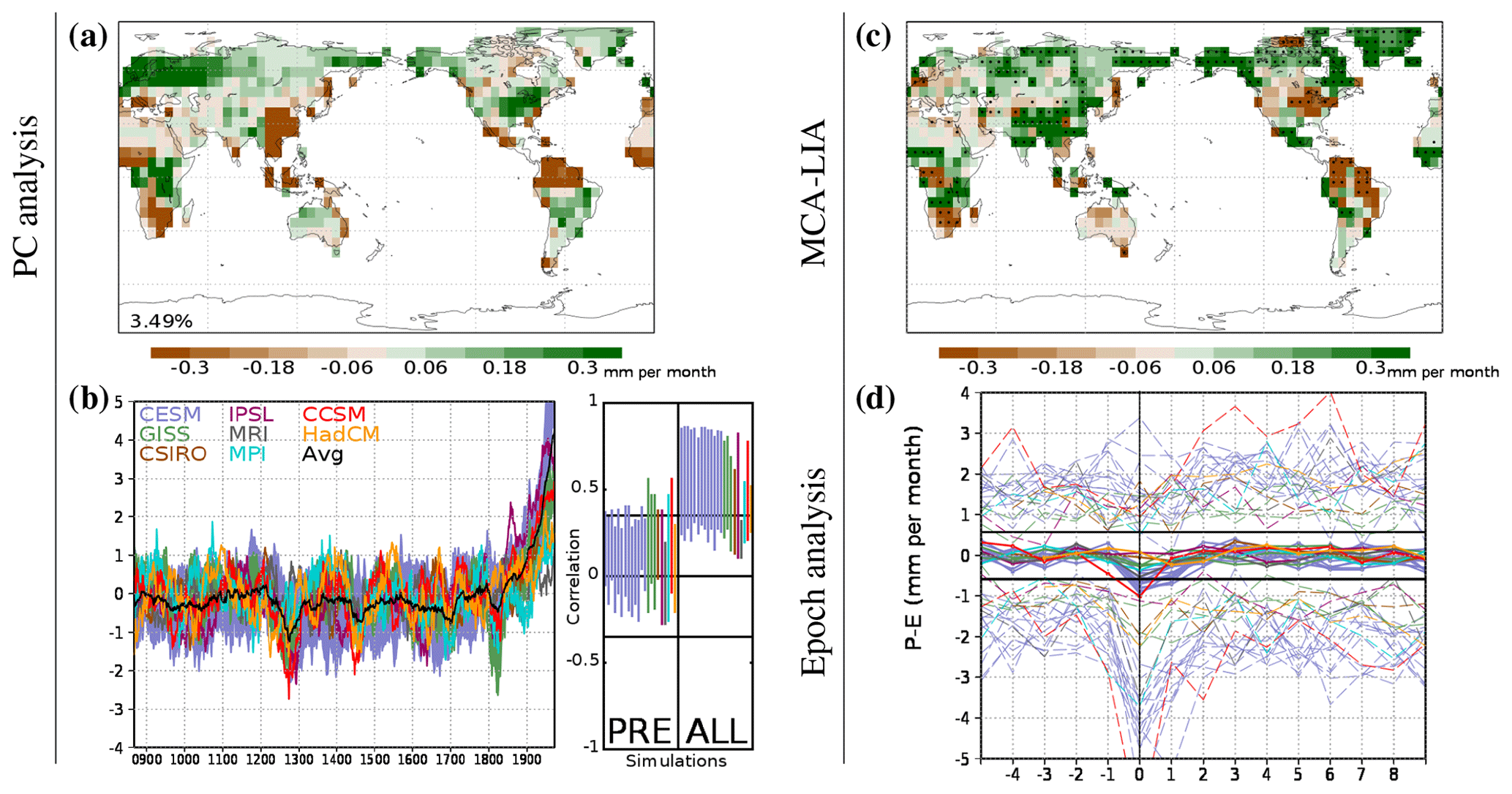
Figure 15 Analysis of P–E for the ensemble of simulations included in Table 1. (a) Second EOF and (b) second PC time series for each simulation, as well as the average PC of all the simulations (black line). The percentage of explained variance is shown within the EOF map. The range of correlations between the PC of each simulation and those of other simulations is also included on the right of the plotted PCs both for the whole period (ALL) and for the preindustrial era (PRE). For these correlations, the significance level (p<0.05) accounting for autocorrelation is shown with a black line. (c) Map of P–E differences between MCA and LIA. Dots indicate locations where the differences are significant (p<0.05). (d) Composite average (solid lines) and maximum and minimum (dashed lines) global P–E anomalies in the 5 years before and 10 years after the 12 main volcanic eruptions of the LM. The vertical line indicates the year of the volcanic event. The horizontal black lines show the significance level of the average (p<0.10) based on the distribution of averages of 12 years generated with 2200 sets randomly taken from the whole period excluding the years of the 12 main volcanic eruptions and the 10 years after them.

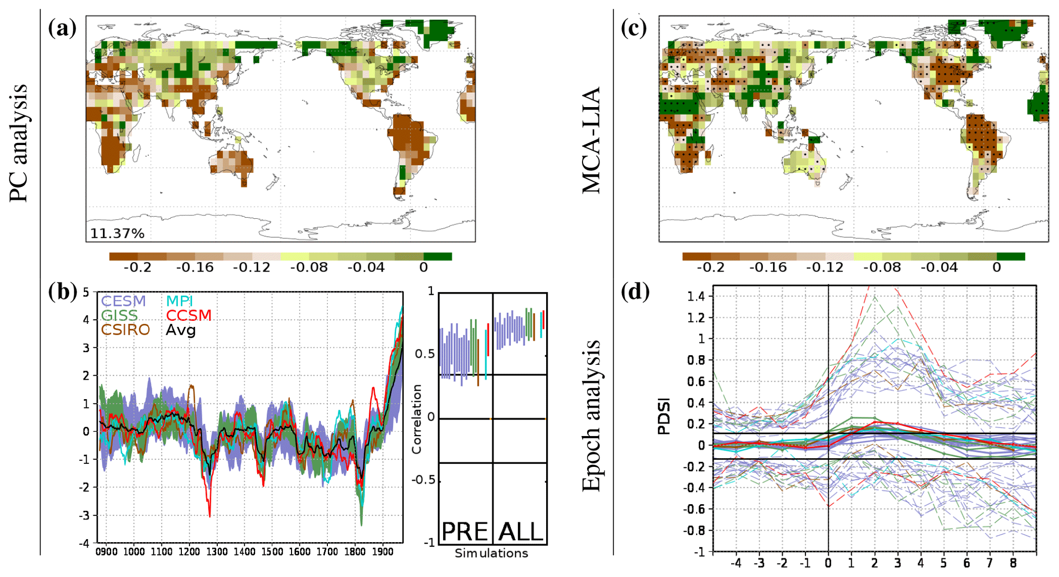
Figure 16 Analysis of scPDSI for the ensemble of simulations included in Table 1. (a) First EOF and (b) first PC time series for each simulation, as well as the average PC of all the simulations (black line). The percentage of explained variance is shown within the EOF map. The range of correlations between the PC of each simulation and those of other simulations is also included on the right of the plotted PCs both for the whole period (ALL) and for the preindustrial era (PRE). For these correlations, the significance level (p<0.05) accounting for autocorrelation is shown with a black line. (c) Map of scPDSI differences between MCA and LIA. Dots indicate locations where the differences are significant (p<0.05). (d) Composite average (solid lines) and maximum and minimum (dashed lines) global scPDSI anomalies in the 5 years before and 10 years after the 12 main volcanic eruptions of the LM. The vertical line indicates the year of the volcanic event. The horizontal black lines show the significance level of the average (p<0.10) based on the distribution of averages of 12 years generated with 2200 sets randomly taken from the whole period excluding the years of the 12 main volcanic eruptions and the 10 years after them.

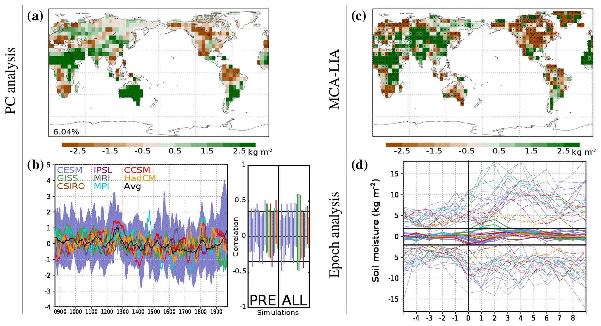
Figure 17 Analysis of soil moisture for the ensemble of simulations included in Table 1. (a) Second EOF and (b) second PC time series for each simulation, as well as the average PC of all the simulations (black line). The percentage of explained variance is shown within the EOF map. The range of correlations between the PC of each simulation and those of other simulations is also included on the right of the plotted PCs both for the whole period (ALL) and for the preindustrial era (PRE). For these correlations, the significance level (p<0.05) accounting for autocorrelation is shown with a black line. (c) Map of soil moisture differences between MCA and LIA. Dots indicate locations where the differences are significant (p<0.05). (d) Composite average (solid lines) and maximum and minimum (dashed lines) global soil moisture anomalies in the 5 years before and 10 years after the 12 main volcanic eruptions of the LM. The vertical line indicates the year of the volcanic event. The horizontal black lines show the significance level of the average (p<0.10) based on the distribution of averages of 12 years generated with 2200 sets randomly taken from the whole period excluding the years of the 12 main volcanic eruptions and the 10 years after them.

Figures 15 to 17 show the modes of P–E, scPDSI, and soil moisture that bear a relationship with global temperature and thus external forcing responses. The associated mode is the second for P–E (Fig. 15) and soil moisture (Fig. 17) and the first for scPDSI (Fig. 16). P–E and scPDSI present PCs that correlate significantly with the temperature response mode (Fig. 2; Table 3); the correlation of the average PC with that of temperature being 0.62 and 0.94 for P–E and scPDSI, respectively. Individual correlations are significant for most simulations and particularly high for those of GISS, IPSL, and CCSM. The highest correlations are attained for scPDSI, being significant and above 0.5 for all simulations, while for soil moisture correlations are lower and in general not significant. The correlations with precipitation (Table 3) are significant for both P–E and scPDSI, being generally higher for P–E. The correlation of the average PC of P–E and scPDSI with that of precipitation reaches values of 0.93 and 0.91, respectively. For P–E and scPDSI there is a clear time response pattern that shows an evolution very similar to that of precipitation (Fig. 11) and temperature (Fig. 2), P–E being more related to precipitation and scPDSI to temperature, as shown in the correlations of Table 3. In the case of P–E, the EOF spatial pattern is similar to that of precipitation (Fig. 11a), showing large negative values over parts of the central American and north of the South American monsoon regions, as well as over the East Asian continent and over parts of the African monsoon regions, where the EOF of precipitation also includes negative loadings. Positive loadings are shown over extratropical continents – in northern Europe, southeastern North America, Alaska, and eastern Siberia – and thus over areas influenced by changes in zonal circulation, which is consistent with the results of the precipitation analyses. As in the case of precipitation, volcanic forcing produces global negative anomalies in the model ensemble that tend to last over 2–3 years.

The scPDSI shows a very similar EOF pattern to that of P–E but with greater emphasis on the negative loadings that dominate over larger scales, extending over Australia, the broader African continent, South America, and large areas of North America and Eurasia (Fig. 16a). Thus, contrary to the P–E and precipitation results, which show more areas with positive anomalies during the 20th century, scPDSI shows negative trends for most regions. Negative scores in the PC during the volcanic episodes, associated with global spread negative loadings, are indicative of wetter soils, and indeed Fig. 16d shows increments in the global average of scPDSI in the model ensemble over timescales of about 5 years. Correlations between various ensemble members are high for P–E (Fig. 15b) if the 20th century trends are considered and lower and often not significant for preindustrial times, indicating the influence of internal variability as in the case of precipitation (Fig. 11b). The scPDSI correlations are, however, significant and high during preindustrial times as well, which is likely a sign of the influence of temperature evolution in this variable. MCA–LIA changes for P–E (Fig. 15c) are very similar to the continental component of the corresponding precipitation pattern (Fig. 11c). As in the case of the EOF loadings, Fig. 16c shows MCA–LIA changes consistent with Fig. 15c though with widespread negative scPDSI values.

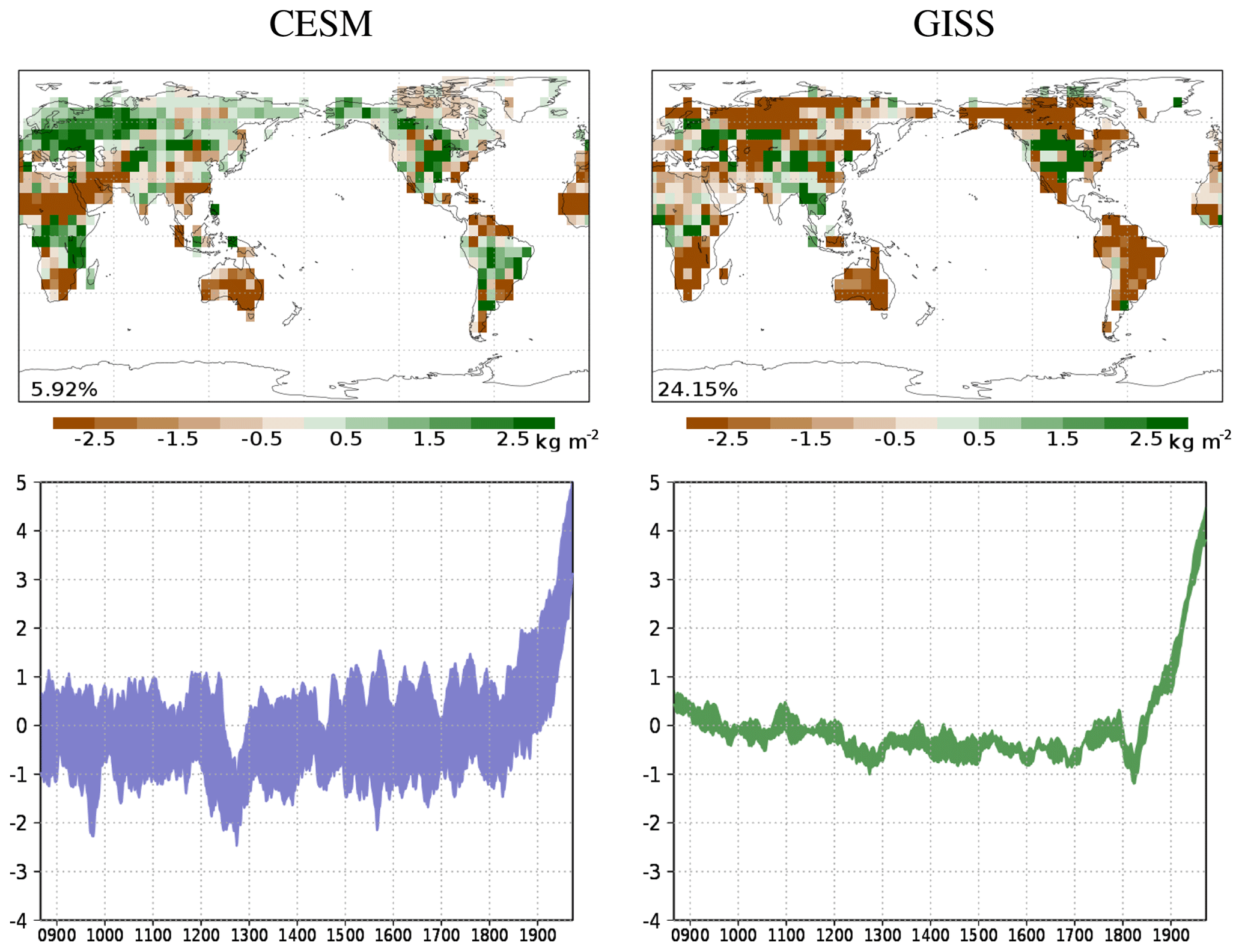
Figure 18 Second EOF and PC of soil moisture for the subensembles of CESM and GISS.

The analysis of soil moisture (Fig. 17) does not show a clear relationship to external forcing, with some of the simulations in the ensemble showing poor correlations with temperature (Table 3). Some sensitivity to volcanic events and 20th century warming is apparent in the behavior of the PC time series. The composite of volcanic eruptions shows some increase in variability in the ensemble but not a clear response to increasing or decreasing soil moisture during volcanic events, indicating that internal variability may dominate over a potential response to the forcing. The associated EOF and MCA–LIA map (Fig. 17a, c) shows similarities to those of Figs. 15a, c and 16a, c with negative values over northern South America and parts of central and southern Africa. Over northern Africa, soil moisture shows positive loadings in the EOF and wetter values in the MCA–LIA differences. Interestingly, all EOF (MCA–LIA) maps in Figs. 15, 16, and 17 show negative (positive) values over eastern Asia and positive (negative) values over eastern North America. Despite an absence of a universal response of soil moisture to external forcing, some of the simulations have clearer responses. This is the case of the CESM and GISS models. When an analysis is carried out independently for these subensembles, the resulting PC series (Fig. 18) show a clear correspondence with the temperature PC. Their corresponding EOFs show, however, considerable spatial differences.

These results suggest that a more focused analysis would be required to address the behavior of drought-related variables and, specifically, soil moisture while also considering more ad hoc techniques and homogeneous definitions of the soil moisture content. Soil moisture, scPDSI, and P–E measure different parts of the hydrological cycle. Additionally, soil moisture behavior during the 20th century may be affected by CO₂ fertilization effects (Mankin et al., 2019) which are not present in other variables such as scPDSI. For this reason, the analyses based on these variables should be considered complementary and not necessarily comparable.

4 Conclusions

This work investigated the response of the current generation of climate models to changes in external forcing during the LM. For this purpose, an ensemble of CMIP5/PMIP3 model simulations is considered, including all natural and anthropogenic forcings during the LM. It is focused on temperature as a reference to identify the response to external forcing and search for consistencies in the behavior of large-scale dynamics and hydrology. Large-scale dynamics were assessed by studying changes in SLP and zonal and meridional wind, while hydrological changes were studied by considering precipitation and drought-related variables. For the latter, P–E, scPDSI, and soil moisture were considered. All variables were studied considering changes at different timescales. PC analysis was used to identify the multi-model typical pattern of response of different variables to the external forcing changes from decadal to multicentennial timescales, MCA–LIA differences are characterized as descriptors of large-scale changes associated with changes in natural forcing during preindustrial times, and volcanic composites are used as indicators of large interannual changes.

The temperature response to forcing depicts a spatial pattern of temperature anomalies that are larger over the continents and polar areas than over oceans. The temporal response of temperature shows changes that follow those of natural forcing during the LM and anthropogenic forcing post-1850. All analyzed variables, both related to dynamics and hydroclimate, show responses that correlate or are consistent with those of temperature. Changes in SLP depict increases (decreases) in the zonal flow in the high latitudes of both hemispheres during times of higher (lower) forcing. Within the tropical regions, zonal and meridional wind components indicate that changes favor convergence and alter the monsoon system. PC time series correlate with those of temperature, and volcanic composites also show sensitivity in these variables. The responses nevertheless can be spatially variable for different models and contribute differently to global averages.

Precipitation changes show a hydrological cycle that is enhanced, which is consistent with the changes in temperature. At middle and high latitudes, precipitation anomalies arise in response to changes in the zonal flow. Within the intertropical regions, precipitation anomalies distribute over monsoon regions and convergence zones, which is consistent with the changes described for climate change scenario simulations. Such large-scale anomalies distribute over different continents, generating covariance in intra- and inter-basin regions. Nevertheless, other modes of internal variability also show widespread inter-basin anomalies and have the potential to contribute to multidecadal and centennial changes in the system.

The analysis of drought-related variables shows dependencies with the definition of the variable itself and its relationship to temperature or precipitation. P–E shows responses that mimic those of precipitation over the continents. Increased P–E values tend to occur with increased forcing over mid- and high-latitude regions influenced by the zonal flow. Within the intertropical regions, the same anomalies for precipitation are simulated over monsoon-sensitive areas. For the MCA–LIA differences, increased drought is simulated over northern South American and southern African monsoon regions, while increased wetness is simulated over the Asian monsoon regions. Unlike P–E, scPDSI shows higher correlations with temperature with spatial patterns that show decreased wetness for most areas during the MCA and industrial period and increased wetness during the LIA. The time evolution of its forcing response mode is very similar to that of temperature, globally producing increased scPDSI (reduced drought) during volcanic composites and contributing to increased drought during the 20th century.

The behavior of soil moisture is more complex and model-dependent. Some models depict clear responses to forcing but with differences in their spatial distribution and time response. The analysis of this variable shows a great dependency on the land models within the climate model itself. A response to external forcing is found when analyzing subensembles of CESM and GISS independently but not in the combined analyses including simulations from different models. This indicates that soil moisture can produce relevant results if a single model is considered, but it is not a suitable variable for analyses involving simulations with different land models.