the Creative Commons Attribution 4.0 License.
the Creative Commons Attribution 4.0 License.
 | 17 Jul 2020
Early Eocene vigorous ocean overturning and its contribution to a warm Southern Ocean
Thierry Huck
Camille Lique
Yannick Donnadieu
Jean-Baptiste Ladant
Marina Rabineau
Daniel Aslanian
The early Eocene (∼55 Ma) was the warmest period of the Cenozoic and was most likely characterized by extremely high atmospheric CO2 concentrations. Here, we analyze simulations of the early Eocene performed with the IPSL-CM5A2 Earth system model, set up with paleogeographic reconstructions of this period from the DeepMIP project and with different levels of atmospheric CO2. When compared with proxy-based reconstructions, the simulations reasonably capture both the reconstructed amplitude and pattern of early Eocene sea surface temperature. A comparison with simulations of modern conditions allows us to explore the changes in ocean circulation and the resulting ocean meridional heat transport. At a CO2 level of 840 ppm, the early Eocene simulation is characterized by a strong abyssal overturning circulation in the Southern Hemisphere (40 Sv at 60∘ S), fed by deepwater formation in the three sectors of the Southern Ocean. Deep convection in the Southern Ocean is favored by the closed Drake and Tasmanian passages, which provide western boundaries for the buildup of strong subpolar gyres in the Weddell and Ross seas, in the middle of which convection develops. The strong overturning circulation, associated with subpolar gyres, sustains the poleward advection of saline subtropical water to the convective regions in the Southern Ocean, thereby maintaining deepwater formation. This salt–advection feedback mechanism is akin to that responsible for the present-day North Atlantic overturning circulation. The strong abyssal overturning circulation in the 55 Ma simulations primarily results in an enhanced poleward ocean heat transport by 0.3–0.7 PW in the Southern Hemisphere compared to modern conditions, reaching 1.7 PW southward at 20∘ S, and contributes to keeping the Southern Ocean and Antarctica warm in the Eocene. Simulations with different atmospheric CO2 levels show that ocean circulation and heat transport are relatively insensitive to CO2 doubling.
- Article
(2070 KB) - Full-text XML
-
Supplement
(1194 KB) - BibTeX
- EndNote


Proxy-based temperature reconstructions suggest that the early Eocene (55–50 Ma) was one of the warmest intervals in geological history and the warmest of the Cenozoic (Zachos et al., 2001; Cramer et al., 2011; Dunkley Jones et al., 2013). More specifically, the EECO (Early Eocene Climatic Optimum) covers the interval between 53 and 51 Ma, but shorter (less than tens of thousands of years) hyperthermal events, such as the PETM (Paleocene–Eocene Thermal Maximum) about 55 Myr ago (Zachos et al., 2008), also spanned the early Eocene. The Southern Hemisphere was particularly warm at that time, as shown by inferred surface ocean temperatures exceeding 20 ∘C at high latitudes (e.g., Evans et al., 2018, and references therein) and by the absence of a perennial ice sheet over Antarctica until the Eocene–Oligocene boundary (∼34 Ma) when CO2 abruptly declined below a certain threshold (Galeotti et al., 2016; Gasson et al., 2014; Ladant et al., 2014). In the early Eocene, high levels of CO2 in the atmosphere were undoubtedly a critical contributor to the extremely warm climate, with the global temperature increasing by more than 5 ∘C in less than 10 000 years (Zachos et al., 2001, 2008; Huber and Caballero, 2011; Anagnostou et al., 2016), but they do not fully explain the extreme warmth at high latitudes and the reduced Equator-to-pole temperature gradient (Huber and Caballero, 2011).
In addition to these much higher levels of CO2 in the atmosphere, one of the main differences between the early Eocene and our modern climate lies in the distinct bathymetric and continental configurations, likely resulting in very different ocean circulation (Thomas et al., 2003; Voigt et al., 2013; Winguth et al., 2012; Zachos et al., 2001). In particular, the opening or closing of major oceanic gateways (such as the Drake Passage or the Panama seaway) during the late Paleogene and Neogene have been shown to exert a strong influence on the ocean circulation and its associated heat transport (England et al., 2017; Ladant et al., 2018; Nong et al., 2000; Sijp and England, 2004; Toggweiler and Bjornsson, 2000; Yang et al., 2014). Additionally, proxy-based reconstructions and results from Eocene model simulations suggest that the Meridional Overturning Circulation (MOC) was also very distinct from our present-day MOC, with no evidence for deepwater formation in the North Atlantic until the early Oligocene (Ferreira et al., 2018). Instead, the formation of deep water is suggested to have happened in the North Pacific (Hutchinson et al., 2018; Winguth et al., 2012) or only in the Southern Ocean (Sijp et al., 2014). Different ocean circulations resulting from different bathymetries are expected to result in different ocean heat transport (OHT). For instance, Sijp and England (2004) found a 0.5 PW decrease in OHT in the Southern Hemisphere in response to the opening of the Drake Passage, but other factors such as CO2-induced radiation may also contribute to altering OHT (see Huber, 2012, for a review).
In our present-day climate, the ocean is an important actor of the Earth energy balance, as it contributes about one-third to the total redistribution of heat from the Equator to the poles (e.g., Trenberth and Caron, 2001). Although modifications of both the atmosphere and the ocean heat transport (OHT) tend to compensate (Trenberth and Caron, 2001), subtle changes in OHT could trigger large changes in atmospheric extratropical convection, modifying water vapor greenhouse (Rose and Ferreira, 2013) and thereby affecting surface temperatures. The OHT itself results from various contributions, and several attempts have been made in the literature to disentangle the relative roles of the horizontal and overturning ocean circulations in the meridional OHT (Ganachaud and Wunsch, 2003). In the North Atlantic, the strong Atlantic Meridional Overturning Circulation (AMOC) is fed by the formation of dense water by convection at high latitudes, and the AMOC contributes up to 90 % of the meridional OHT at 26.5∘ N (Msadek et al., 2013), where the RAPID monitoring array is located (McCarthy et al., 2015). Based on hosing experiments performed with a climate model (FAOM), Yang et al. (2013) found that the meridional OHT decreases rapidly in response to an artificial shutdown of the AMOC, although Drijfhout and Hazeleger (2006) suggested that on a longer (decadal) timescale, the OHT might recover its initial level as the gyre contribution tends to compensate for the decrease in OHT associated with the AMOC shutdown. In contrast to the North Atlantic, Volkov et al. (2010) found that, in the Southern Ocean, the OHT results roughly equally from the gyre and overturning contributions.
Given the importance of both horizontal and overturning ocean circulations for the meridional OHT, the different MOC and horizontal gyres constrained by the Eocene bathymetry may result in different contributions to the meridional OHT and may potentially contribute to the warm early Eocene climate, in particular in the much warmer high latitudes. Based on the analysis of early Eocene and present-day simulations performed with the IPSL-CM5A2 Earth system model, the goal of this study is to better understand what sets the Eocene ocean circulation and the importance of the ocean circulation for the poleward heat transport. The model and simulations used are described in Sect. 2. In Sects. 3 and 4, we examine the MOC and the horizontal circulation, respectively, for the present-day and 55 Ma configurations, and these circulations are then linked to the OHT in Sect. 5. The sensitivity of the ocean circulation and heat transport to the level of CO2 in the atmosphere is discussed in Sect. 6. A summary and conclusions are given in Sect. 7.
2.1 Model setup and simulations
The simulations used in this study are performed with the IPSL-CM5A2 Earth system model (Sepulchre et al., 2019). The oceanic component of IPSL-CM5A2 is NEMOv3.6 (Madec and the NEMO team, 2016), which includes the LIM2 sea ice model (Fichefet and Maqueda, 1997) and the PISCES biogeochemical model (Aumont et al., 2015). The atmospheric component is the LMDZ model (Hourdin et al., 2013), which is coupled to the land surface model ORCHIDEE (Krinner et al., 2005). Here, we use IPSL-CM5A2 in its standard resolution. NEMO is thus run at a nominal resolution of 2∘, increased down to 0.5∘ at the Equator, with 31 levels that vary in thickness with depth. LMDZ is run at a horizontal resolution of 3.75∘ longitude latitude and 39 vertical levels. A full description and evaluation of the IPSL-CM5A2 model can be found in Sepulchre et al. (2019).
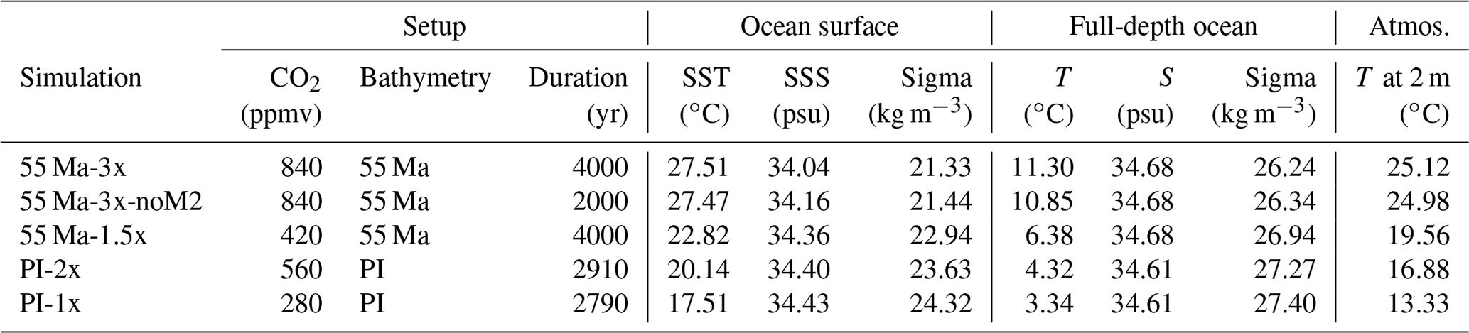
Two sets of simulations are performed. The first set is composed of the reference preindustrial (PI) simulation (referred to as PI-1x and described in Sepulchre et al., 2019) and another PI simulation in which the atmospheric CO2 concentration is doubled (PI-2x). The second set consists of a baseline simulation of the early Eocene (hereafter 55 Ma-3x) using a setup following the DeepMIP protocol described by Lunt et al. (2017) and two sensitivity experiments to a reduced CO2 level (55 Ma-1.5x) and to no tidal mixing (55 Ma-noM2). In the following, we first briefly describe the baseline early Eocene simulation (as the DeepMIP guidelines from Lunt et al. (2017) give several options for implementing the early Eocene boundary conditions) and then make the boundary condition differences of the two other simulations precise.
2.1.1 General considerations
Most of the boundary conditions that were adapted for these IPSL-CM5A2 early Eocene simulations are described in Herold et al. (2014, hereafter H14). Following Lunt et al. (2017), the solar constant and orbital parameters are kept to PI values; so are greenhouse gas concentrations with the exception of atmospheric CO2. The latter is set to 840 ppm (3 times the PI value) so that the simulation is representative of the pre-PETM (following the terminology of Lunt et al., 2017).
2.1.2 Oceanic boundary conditions
The ocean component (NEMO) is commonly run on a tripolar mesh grid (Madec and the NEMO team, 2016), which avoids singularity points in the ocean domain. Because the implementation of the Eocene land–sea mask on the ORCA2 grid would have shifted the singularity points into the ocean domain, we have constructed a new PALEORCA grid, which is designed to run paleo-simulations with IPSL-CM5A2 (see more details in Sepulchre et al., 2019). The bathymetry is obtained by masking out the H14 topography and remapping the resulting bathymetry onto the PALEORCA grid using nearest-neighbor interpolation. This type of interpolation indeed ensures that small but crucial features of the H14 dataset such as islands and seaways, which may strongly impact the modeled ocean circulation, remain present in the interpolated bathymetry file. Manual corrections have then been applied at some locations (e.g., in the West African region) to retain oceanic straits that are sufficiently large to allow for exchanges. The early Eocene bathymetry is shown in Fig. 1.
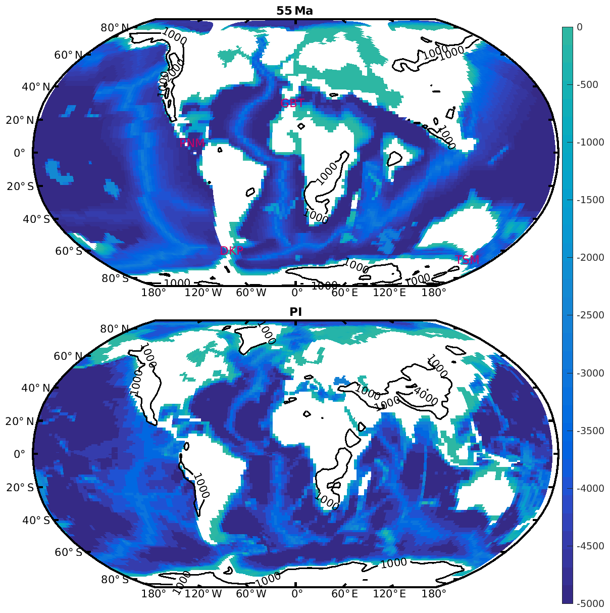
Figure 1Bathymetry and topography (m) boundary conditions used in the 55 Ma (based on Herold et al., 2014) and PI simulations. The black contours indicate 1000 and 4000 m of altitude. DKP indicates the Drake Passage, TSM the Tasmanian Passage, PNM the Panama passage and GBT Gibraltar.
Modern boundary conditions of NEMO also include forcings of the dissipation associated with internal wave energy from the M2 and K1 tidal components (de Lavergne et al., 2019). The parameterization follows Simmons et al. (2004), with refinements in the modern Indonesian throughflow (ITF) region according to Koch-Larrouy et al. (2007). To create an early Eocene tidal dissipation forcing, we directly interpolate the H14 M2 tidal field (obtained from the tidal model simulations of Green and Huber, 2013) onto the NEMO grid using bilinear interpolation. In the absence of any estimation of the K1 tidal component for the early Eocene, we ignore this contribution. In addition, the parameterization of Koch-Larrouy et al. (2007) is not used here because the ITF did not exist in the early Eocene.
The geothermal heating distribution q is created from the 55 Ma global crustal age distribution of Müller et al. (2008), on which the age–heat-flow relationship of the Stein and Stein (1992) model is applied.
In regions of subducted seafloor where age information is not available, we prescribe the minimal heat-flow value derived from known crustal age. The resulting field is then bilinearly interpolated on the NEMO grid. It must be noted that the Stein and Stein parameterization becomes singular for young crustal ages, which yields unrealistically large heat-flow values. We thus set an upper limit of 400 mW m−2 on heat-flow values, following Emile-Geay and Madec (2009).
Salinity is initialized as globally constant to a value of 34.7 psu following Lunt et al. (2017). The initialization of the model with the proposed DeepMIP temperature distribution (Lunt et al., 2017) led to severe instabilities of the model during the spin-up phase. The initial temperature distribution has thus been modified to follow
with φ the latitude and z the depth of the ocean. This new equation gives an initial globally constant temperature of 10 ∘C below 1000 m and a zonally symmetric distribution above, reaching surface values of 35 ∘C at the Equator and 10 ∘C at the poles. This profile gives a 5 ∘C surface temperature reduction compared to the DeepMIP equation (Lunt et al., 2017). No sea ice is prescribed at the beginning of the simulations.
The IPSL-CM5A2 model includes the PISCES biogeochemical model. Biogeochemical cycles and marine biology are directly forced by dynamical variables of the physical ocean and may affect the ocean physics via their influence on chlorophyll production, which modulates light penetration in the ocean. However, because this feedback does not significantly affect the ocean state significantly (Kageyama et al., 2013) and because the early Eocene mean ocean color is unknown, we have prescribed a constant chlorophyll value of 0.05 g Chl L−1 for the computation of light penetration in the ocean. As a consequence, marine biogeochemical cycles and biology do not alter the dynamics of the ocean, and as such, biogeochemical initial forcings have been kept to modern.
2.1.3 Continental boundary conditions
The atmospheric (LMDZ) and land surface (ORCHIDEE) models run on a low-resolution grid but require input forcings at higher resolution. The topographic field is created by masking out ocean points in the H14 reference file and upscaling the masked H14 file to the required LMDZ input topographic resolution (1/6∘), as LMDZ includes a subgrid-scale orographic drag parameterization requiring high-resolution surface orography (Lott and Miller, 1997; Lott, 1999). A similar procedure is applied to the standard deviation of orography proposed by H14.
Following Lunt et al. (2017), the soil properties are prescribed as globally constant to the global mean of the PI simulation. There is no lake module in this version of IPSL-CM5A2. The river routing proposed by H14 is passed to ORCHIDEE at its original resolution of , which ensures an appropriate downscaling to the model resolution. The vegetation cover is prescribed from the BIOME4 reconstruction of H14 using a lookup table (given in Table S2) to convert the 10 megabiomes into ORCHIDEE plant functional types (PFTs). Aerosol distributions are left identical to PI values.
Table 1Summary of the simulation setup and key diagnostics in the different simulations used in this study. All the values presented are averaged over the last 100 years of each simulation.
2.1.4 Sensitivity experiments and equilibrium
We perform two additional early Eocene experiments. One has the same boundary conditions as the baseline early Eocene experiment (55 Ma-3x) but an atmospheric CO2 concentration of 420 ppm (1.5 times the PI levels, 55 Ma-1.5x). The other differs from the baseline early Eocene experiment by the absence of tidal dissipation forcing (55 Ma-3x-noM2).
The 55 Ma-3x simulation is initialized from rest and run for 4000 years (Fig. S1 in the Supplement). The 55 Ma-1.5x simulation is branched from 55 Ma-3x at year 1500 and run for 4000 years. The 55 Ma-3x-noM2 is branched from 55 Ma-3x at year 3000 and run for 2000 additional years. The two PI simulations are initialized from the Levitus climatology (Boyer et al., 2005) and run for more than 2700 years (Table 1). At the end of all the simulations, the ocean has reached a quasi-equilibrated state and trends in deep ocean temperatures over the final 1000 years of all simulations are smaller than 0.05 ∘C per century.
We use the monthly outputs of the last 100 years of each simulation to create a climatological year for each simulation. In the following, we will mostly focus on the comparison between the baseline early Eocene simulation (55 Ma-3x) and the PI control simulation (PI-1x). The other simulations are analyzed in Sect. 3 to estimate the contribution of tidal mixing to the oceanic overturning circulation and in Sect. 6 to examine the sensitivity of the ocean conditions to different levels of CO2 in the atmosphere.
2.2 Evaluation of the simulated ocean temperature
This section examines the mean state and the seasonal variation of ocean temperature in the 55 Ma simulations. Further, we evaluate the ability of IPSL-CM5A2 to reasonably simulate the early Eocene sea surface temperature (SST).
The annual mean SST in the 55 Ma-3x simulation varies from 10–15 ∘C in the Southern Ocean to 37.2 ∘C near the Equator (Fig. 2a), with a global mean of 27.5 ∘C. During summer (defined as July–August–September for the Northern Hemisphere and January–February–March for the Southern Hemisphere), the simulated SST reaches ∼20 ∘C over most of Southern Ocean (south of 60∘ S) and up to 38 ∘C in parts of equatorial Indian and Atlantic oceans (Fig. 2a). In the 55 Ma-1.5x simulation, both SST and global mean temperature are ∼5 ∘C lower than in the 55 Ma-3x simulation (Table 1).
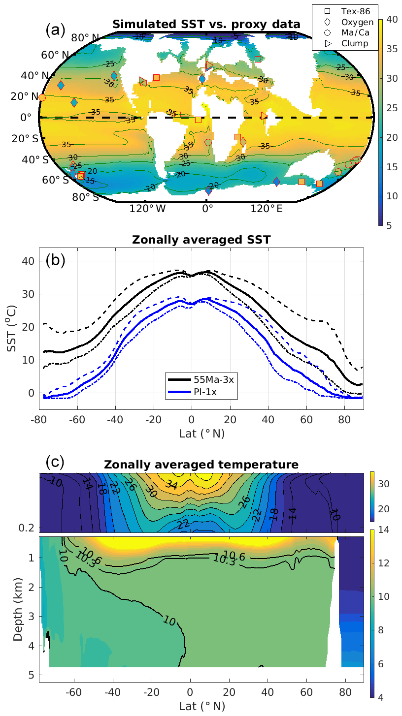
Figure 2(a) Annual mean SST (∘C) in the 55 Ma-3x simulation and point-to-point comparisons with proxy-based SST estimates from the DeepMIP dataset for the early Eocene (Hollis et al., 2019). The different symbols represent different proxies. (b) Simulated zonally averaged annual mean SST (∘C, solid lines) in the 55 Ma-3x (black) and PI-1x (blue) simulations. The dashed and dotted lines indicate the means for summer and winter, respectively. (c) Zonally averaged ocean temperature in the 55 Ma-3x simulation, with a zoom of the upper 200 m (contour interval: 2 and 0.3 ∘C for the upper and lower parts of panel c, respectively).
These simulated SSTs are further compared with proxy-based SST estimates for the early Eocene provided by a recent data compilation performed within the DeepMIP framework (Hollis et al., 2019). The dataset includes 32 records in total from four proxy types (TEX86, δ18O, Mg∕Ca and clumped isotope data). The spatial pattern of the simulated SST is overall consistent with the proxy-based SST, although significant differences can be observed at some specific proxy data sites (Figs. 2a and S2a).
Table 2Root mean square deviation (RMSD) of simulated annual mean SST and proxy-based SST estimates (∘C) at 55 Ma. RMSD metrics are defined in the Supplement. The proxy-based SST estimates are from the DeepMIP dataset for the early Eocene (Hollis et al., 2019), and the number of data points and the uncertainty for each proxy type are also indicated. The uncertainty range is defined as the 2σ deviations for δ18O and as the range between the 5th and 95th percentile SST estimates for TEX86, Mg∕Ca and clumped isotope data.
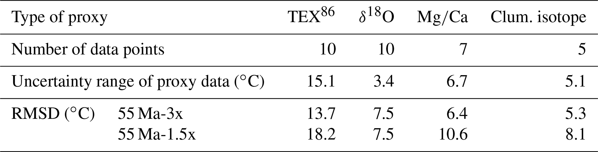
In order to further compare the simulations with the proxy-based reconstructions, we also calculate the root mean square deviations (RMSDs) between the simulated SST and the reconstructions (Table 2). Although large, the RMSD values are overall of the same order of magnitude as the uncertainties of proxy-based SST estimates, suggesting a reasonable model–data consistency. More importantly, the RMSD values are smaller for the 55 Ma-3x simulation than for the 55 Ma-1.5x simulation, suggesting that the 55 Ma-3x simulation better captures the signal of proxy-based SST reconstructions. This is also consistent with proxy reconstructions suggesting that the atmospheric CO2 concentrations during the early Eocene were most likely 3 to 4 times the PI level (Foster et al., 2017). Additional details on the model–proxy comparison can be found in the Supplement.
The zonal mean SST in the 55 Ma-3x simulation ranges from 30 to 37 ∘C in the tropics and decreases toward the high latitudes (Fig. 2b). Within the 40∘ S–40∘ N latitudinal band, summer SST remains above 30 ∘C, whereas around 60–70∘ S the annual mean SSTs are ∼13 ∘C, with a seasonal amplitude of 10 to 15 ∘C. These zonal mean SSTs are overall ∼10 ∘C warmer than in the PI-1x simulation, with the largest warmings (as much as 12 ∘C) found in the Southern Ocean (Fig. 2b). The warm SSTs found in the Southern Ocean in the 55 Ma simulations also extend at depth (Fig. 2c), with a mean global temperature of 11.3 ∘C in the 55 Ma-3x run compared to 3.3 ∘C in PI-1x (Table 1). The very warm temperatures found at depth are compatible with several proxy-based temperature estimates (bottom temperatures at 1000–5000 m between 10 and 15 ∘C; e.g., Huber et al., 2000, their Fig. 4-1). More specifically, Mg∕Ca-based temperature estimates suggest that the bottom-water (below 1000 m) temperatures were around 15 ∘C during the early Eocene (Cramer et al., 2011), and Dunkley Jones et al. (2013) found a similar value based on δ18O-Mg∕Ca paleo-thermometry for the PETM time window.
Here we describe the simulated MOC in the different simulations and investigate the links between the MOC and deepwater formation.
3.1 Meridional overturning circulation
The global MOC is represented through the vertical streamfunction ψ computed from the zonally integrated meridional volume transport as
where v is the meridional velocity, y is the latitude, z is the vertical coordinate and x is the zonal coordinate integrated from the west (W) to east (E) boundary (meaning that we examine ψ while facing west).
Table 3Key ocean surface parameters in the North Pacific and Weddell Sea in 55 Ma-3x simulation. The Weddell Sea and the North Pacific convection regions are defined by the deepest mixed layer depth at high latitudes, and the extended regions are defined as boxes over the Weddell Sea (78–61∘ S and 62∘ W–8∘ E) and the North Pacific (48–67∘ N and 124∘ E–143∘ W) roughly corresponding to closed contours of sea surface height. SST, sea surface salinity (SSS) and sigma are winter averages (January–February–March for the Northern Hemisphere and July–August–September for the Southern Hemisphere), and MLD is given for the end of winter (March for the Northern Hemisphere and September for the Southern Hemisphere), while precipitation, runoff and evaporation are annual means.
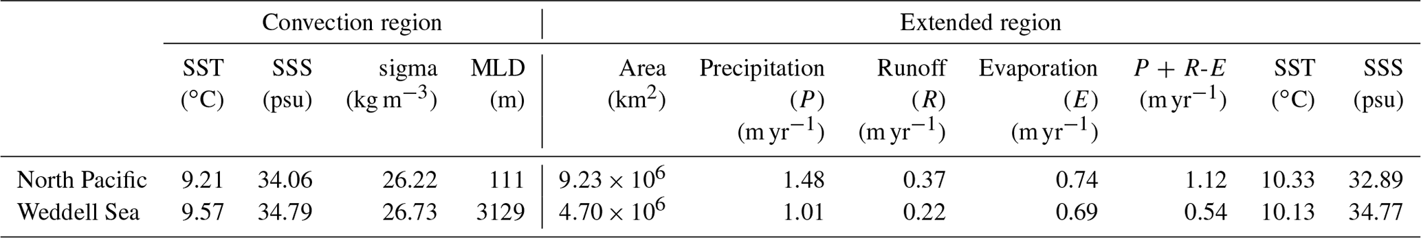

Figure 3Streamfunction of the meridional overturning circulation (Sv) in the 55 Ma-3x (a, contour interval: 4 Sv) and PI-1x (b, contour interval: 2 Sv) simulations. Note the different color bars of the two subplots. The thick black lines indicate the zero contour, with positive values indicating clockwise circulation and negative values anticlockwise circulation. White lines show selected zonally averaged isopycnal contours (potential density: kg m−3).
In the 55 Ma-3x simulation, a single anticlockwise interhemispheric MOC cell fills the whole deep ocean, with a maximum of 40 Sv at 1500 m of depth and 60∘ S (Fig. 3). This strong MOC cell (referred to as SOMOC for Southern Ocean MOC) is associated with the formation of (Eocene) Antarctic Bottom Water (AABW) in the Southern Ocean, flowing northward below about 2000 m. The SOMOC is associated with an upwelling branch extending over the whole Northern Hemisphere, with almost 26 Sv crossing the Equator northward (22 Sv at 20∘ N and only ∼5 Sv at 60∘ N). There is no deepwater formation in the Northern Hemisphere, neither in the North Atlantic nor in the North Pacific.
In contrast to the 55 Ma-3x run, the MOC in the PI-1x simulation is composed of the traditional upper and lower cells. The upper cell is clockwise and associated with the AMOC, with a maximum strength of 11–12 Sv reached at 800 m of depth around 50–60∘ N. This cell is fed by the formation of North Atlantic Deep Water (NADW) around 60∘ N. NADW is transported southward all the way to the Southern Ocean at depth between 1000 and 3000 m, where it is brought back to the surface through wind-induced upwelling, forming the quasi-adiabatic pole-to-pole overturning circulation regime (Marshall and Speer, 2012; Wolfe and Cessi, 2014). The lower cell is anticlockwise, with a maximum strength of 15–16 Sv at 3000 m of depth. This anticlockwise circulation is fed by the Antarctic Bottom Water formed by surface buoyancy loss related to ocean–sea–ice interaction (Abernathey et al., 2016) and consumed through mixing processes induced by the breaking of internal waves at the seafloor and geothermal heating (Nikurashin and Ferrari, 2013; de Lavergne et al., 2016).
The simulated deepwater formation in the Southern Ocean in the 55 Ma simulation is compatible with currently available proxy-based reconstructions of the MOC. Although proxy data constraining the ocean circulation are very limited for the early Eocene, these data seem to point to a common deepwater source around the Austral Ocean during that period (Abbott et al., 2016; Batenburg et al., 2018; Frank, 2002; Thomas et al., 2003, 2014). For instance, Batenburg et al. (2018) reported the convergence of the Nd isotopic signature of seawater across the Atlantic basin from 59 Ma onward and proposed that this convergence is a result of an intensification of the intermediate and deep ocean circulation in the Atlantic Ocean, with the dominant deepwater mass originating from the southern high latitudes. In addition, the reconstructed concentration of the deep-sea carbonate ion ([]) during the Eocene shows a reversed inter-basin gradient compared to the present day, suggesting a reversed ocean circulation at depth compared to the present-day circulation (Zeebe and Zachos, 2007). Therefore, these proxy data and the simulated ocean circulation are compatible, at least on the direction of the deep circulation and the source of the deepwater masses.
3.2 Convection and deepwater formation
The abyssal circulation described in Sect. 3.1 is fed by deep convection processes that mainly occur in winter. We examine the simulated mixed layer depth (MLD) at the end of the winter season (Fig. 4), which is an efficient indicator of convection. In the 55 Ma-3x simulation, deep convection occurs only at high latitude in the Southern Hemisphere, with maximum MLD reaching up to 4000 m in the Weddell Sea and large areas of MLDs deeper than 2000 m around Antarctica in the Ross and Amundsen seas (Fig. 4). In contrast, MLDs remain shallow in the Northern Hemisphere, suggesting the absence of any deep convection there. In this hemisphere, the maximum MLDs are found in the North Pacific (350 m) over the poleward western boundary current between 35 and 50∘ N and in the North Atlantic between 35 and 40∘ N (300 m), but the deepest MLDs at high latitude are only 200 m over the northwest Pacific. Note that the early Eocene North Atlantic basin is limited to a narrow region west of Greenland and poleward of 52∘ N. In the absence of other sources of deep waters, waters sourced in the Southern Ocean around Antarctica fill the whole abyssal ocean (Fig. 3).
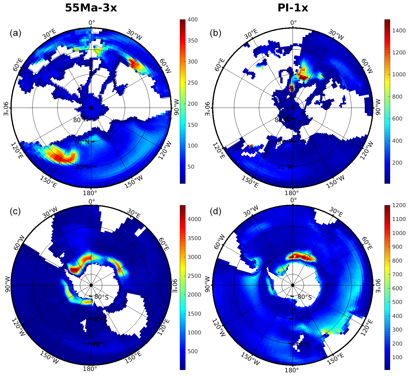
Figure 4Winter (i.e., March in the Northern Hemisphere – a, b; and September in the Southern Hemisphere – c, d) mixed layer depth (m) in the 55 Ma-3x (a, c) and PI-1x (b, d) simulations. Note the very different color bars among plots. Mixed layer depth is defined by the potential density difference of 0.3 kg m−3 with reference to the surface.
In contrast, deepwater formation occurs in both the northern North Atlantic and in the Weddell Sea in the PI-1x simulation (Fig. 4b, d). The deepest MLDs (up to 1500 m) are found in the Nordic Seas between 70 and 75∘ N and just south of Iceland around 60∘ N. MLDs larger than 1200 m are also found in the eastern Weddell Sea around 65∘ S, indicative of the formation of AABW. This pattern is consistent with the MLD simulated by the CMIP5 ensemble for modern conditions (Heuzé et al., 2015).
In 55 Ma-3x, the permanent absence of deep convection in the North Pacific is at odds with a few previous model studies and proxy-based reconstructions of the ocean circulation of the early Eocene that have suggested that deep water could form in the North Pacific (Lunt et al., 2010; Abbott et al., 2016). The reasons why deep water forms in the Southern Ocean in the 55 Ma-3x simulation and not in the North Pacific can be linked to the different ocean thermodynamical properties of these two regions. Table 3 summarizes key ocean surface variables in the convective regions of the Weddell Sea, where the deepest MLDs are found, and of the North Pacific. These two regions roughly correspond to closed sea surface height (SSH) contours around deep convection regions, which are associated with a minimum of SSH – the geostrophic ocean surface currents circulate cyclonically along the SSH contours so that the interior regions remain largely isolated from surrounding waters. The Weddell Sea is characterized by a strongly reduced vertical stratification compared to the North Pacific, the surface signature of which is much larger surface density (+0.51 kg m−3). This reduced stratification provides favorable conditions for the emergence of deep convection. According to the equation of state of seawater, the larger surface density found in the Weddell Sea convection region is due to higher salinity (+0.73 psu) contributing to a density increase of 0.57 kg m−3, partly balanced by a warmer temperature (+0.36 ∘C) contributing to a 0.06 kg m−3 density decrease.
Two major causes may explain these large differences in salinity between the two regions: (i) the atmospheric circulation and freshwater fluxes to the ocean and (ii) the ocean circulation and positive salt–advection feedback. The surface freshwater budget for two extended regions over the Weddell Sea (78–61∘ S and 62∘ W–8∘ E) and the North Pacific (48–67∘ N and 124∘ E–143∘ W) is shown in Table 3. Averaged precipitation and runoff in the North Pacific box (respectively 1.48 and 0.37 m yr−1) exceed those in the Weddell Sea box (1.01 and 0.22 m yr−1) by roughly 50 %, whereas the evaporation rates are almost similar (0.74 vs. 0.69 m yr−1). Overall, the average net surface freshwater input is 0.54 m yr−1 in the Weddell Sea compared to 1.12 m yr−1 in the North Pacific. Reduced freshwater input by precipitation and continental runoff is related to different atmospheric circulation in the Northern and Southern Hemisphere. In the Southern Ocean, winds largely follow the Antarctic orography (as shown by geopotential height at 850 hPa; Fig. S3) and induce almost no precipitation by orographic uplift over Antarctica coastal regions and no runoff to the Southern Ocean. In contrast, in the North Pacific, the westerlies are blocked by the paleo-Rocky Mountains, especially in the region between 50 and 70∘ N. The orographic uplift of moist air masses induces high precipitation (up to 2–3 m yr−1) and runoff into the North Pacific (as found in several other models; Carmichael et al., 2016), leading to low sea surface salinity (below 30 psu) along the Pacific coast of North America (not shown) and consequently to increased surface stratification. The upper branch of the MOC and the associated poleward advection of saline subtropical waters constitute the other contribution to the larger salinities found in the Southern Ocean relative to the North Pacific. This process was sorted out as a positive salt–advection feedback by Ferreira et al. (2018)
In contrast, present-day circulation, characterized by deepwater formation in the North Atlantic, is maintained by higher salinities in the North Atlantic than in the North Pacific, which are partly sustained by atmospheric fluxes and the salt–advection feedback (Ferreira et al., 2018). A recent sensitivity study of the impact of topography on modern ocean circulation reveals that the presence of the Rocky Mountains influences the global salinity pattern and the regions where deep convection occurs through adjustments of the freshwater transfers between the Pacific and Atlantic Ocean (Maffre et al., 2018).
3.3 Factors contributing to the vigorous SOMOC
Different factors contribute to the intense SOMOC simulated by the 55 Ma-3x simulation (40 Sv) in comparison with typical present-day MOC, the intensity of which reaches around 18 and 20 Sv for the upper and lower cells, respectively (Lumpkin and Speer, 2007). Deepwater formation occurs in the three sectors of the Southern Ocean (Pacific, Atlantic and Indian), but the zonal connections between the different basins hamper a clear quantification of the contribution of each deepwater formation sector to the SOMOC. However, the contributions of the Weddell Sea and the Pacific sector of the Southern Ocean can be estimated because the narrow width of the Drake and Tasmanian passages at 55 Ma (Fig. 1) creates latitudinal continental boundaries on the western and eastern sides of these regions. The Weddell Sea, which exhibits the largest MLD in 55 Ma-3x, and the Pacific sector contribute roughly equally to the SOMOC intensity (∼19 Sv). The southern Indian sector contribution is more difficult to assess directly because of the large open-ocean zonal connection with the Atlantic sector.
The shallow Drake Passage at 55 Ma provides a western boundary for the development of a subpolar gyre in the Weddell Sea (see Sect. 4 for more details). This clockwise gyre produces a favorable environment to trigger deepwater formation (known as preconditioning) through isopycnals doming in the center of the gyre, thereby bringing weakly stratified waters of the ocean interior close to the surface (Marshall and Schott, 1999). Clockwise subpolar gyres, and associated deepwater formation by winter convection, are also present in the Pacific sector of the Southern Ocean in the Ross and Amundsen seas. Previous numerical investigations of the effects of a closed Drake Passage on ocean dynamics have revealed that the closure of the Drake Passage tends to promote the existence of subpolar gyres in the Southern Ocean and vigorous deepwater formation (Nong et al., 2000; Sijp and England, 2004; Ladant et al., 2018). Additionally, it has been recently suggested that the effects of the closure and opening of the Drake Passage and the Panama seaway may not be independent (Yang et al., 2014; England et al., 2017; Ladant et al., 2018). For instance, Yang et al. (2014) found that closing the Drake Passage tends to suppress the AMOC and to promote the emergence of a strong SOMOC when the Panama gateway is open, whereas the AMOC may remain intense when the Panama gateway is closed. It is thus very likely that, in our 55 Ma simulations, the very shallow Drake Passage, possibly in combination with the opened Panama gateway, contributes to the strong SOMOC.
In addition to the influence of the different gateways, tidally induced mixing, which represents enhanced vertical diffusivity resulting from breaking internal waves generated by the interaction of tidal currents with rough bottom topography (St. Laurent et al., 2002), is another factor that contributes to the strong SOMOC found in the 55 Ma-3x simulation. A twin experiment of the 55 Ma-3x simulation, in which no tidal-induced mixing is prescribed (55 Ma-3x-noM2), simulates a SOMOC with a similar structure but an intensity that is 7 Sv weaker (33 Sv compared to 40 Sv in the reference 55 Ma-3x simulation; Fig. S4). It should be noted that the additional simulation has only been run for 2000 years, so a small part of the difference between the two runs could arise from different equilibrium states. Yet, the difference between these two simulations is consistent with the recent results of Weber and Thomas (2017), who find a 10 Sv MOC enhancement in an early Eocene simulation with the ECHAM5/MPIOM model that explicitly simulates tides compared with a simulation that does not. This suggests that our parameterization for tidally induced mixing based on the M2 dissipation fields of Green and Huber (2013) reasonably represents the effect of early Eocene tides on global ocean circulation. The strengthening of the MOC induced by tidal mixing can be directly related to the driving role of diapycnal mixing on the overturning circulation. Numerous studies have demonstrated that both the magnitude and the vertical distribution of diapycnal mixing largely affect the strength of the MOC (Bryan, 1987; Manabe and Stouffer, 1999). As already pointed out by Green and Huber (2013), the Eocene MOC may have been much more sensitive to the intensity of the abyssal mixing than the present-day AMOC, which is largely isolated from the ocean floor by the presence of AABW and sustained quasi-adiabatically by the wind-driven upwelling in the Antarctic Circumpolar Current (ACC; Marshall and Speer, 2012). Diapycnal mixing is the only process that can warm up the dense waters formed in the Eocene Southern Ocean, and these dense waters are directly exposed to the tidally induced mixing at the bottom such that the abyssal dissipation becomes the main controlling factor of the SOMOC intensity. In this respect, the large tidal dissipation rate suggested by Green and Huber (2013) in the Pacific is particularly important.
Another often-mentioned factor affecting ocean circulation is the climate state in response to the atmospheric CO2. Based on highly simplified models, theoretical studies have suggested that ocean ventilation tends to increase under a warmer climate state due to a higher sensitivity of seawater density to temperature (e.g., de Boer et al., 2007). However, deepwater formation is a very regional phenomenon, and thus this idealized relationship might be complicated by other regional-scale factors. Indeed, we do not see any systematic change in SOMOC between two simulations with different CO2 levels (1.5 times and 3 times) (see Sect. 6 for a further discussion).
In the present-day North Atlantic, vertical and horizontal circulations are intimately connected, especially in the subpolar gyre (Marshall and Schott, 1999). For instance, the warm North Atlantic Current flowing northward and the cold East Greenland Current flowing southward are found roughly at the same depth at 60∘ N such that the MOC in z coordinates does not capture the associated water mass transformation at high latitude, whereas the MOC in density coordinates does (Zhang, 2010). It is only when the cold branch deepens in the Labrador Sea and becomes the Deep Western Boundary Current off Cape Hatteras that the overturning streamfunction in z coordinates provides a good estimate of the water mass transformation. From this perspective, the horizontal subpolar gyre is an integral part of the North Atlantic thermohaline circulation. By analogy, a similar intricacy between horizontal gyres and the thermohaline circulation can be expected to have existed in the early Eocene Southern Ocean, where the near closure of the Drake and Tasmanian passages allowed for the emergence of intense subpolar gyres, which can precondition and feed the formation of deep water sustaining a strong SOMOC. We thus examine in the following the horizontal ocean circulation during the Eocene.
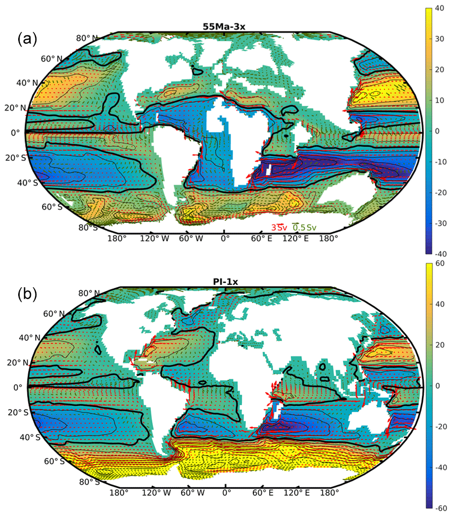
Figure 5Barotropic streamfunction (Sv) in the 55 Ma-3x (a, contour interval: 10 Sv) and PI-1x (b, contour interval: 15 Sv) simulations, integrated northward from Antarctica. Note the different color bars of the two subplots. The thick black lines indicate the zero contour. The mean transport (Sv) integrated over the top 300 m is indicated with vectors (note that only one of every two points is plotted to increase readability). Two scales are used to represent transport larger (in red) or lower (in green) than 0.5 Sv. The transports through the key gateways in the 55 Ma-3x simulation are the Drake Passage (3.1 Sv), Tasmania (1.3 Sv), Panama (4.7 Sv) and Gibraltar (−14.3 Sv) (positive transports are eastward, negative westward). The Drake Passage throughflow, corresponding to ACC, in the PI-1X simulation is ∼108 Sv.
4.1 Gyre circulations
In the 55 Ma-3x run, several horizontal gyres are well developed in both hemispheres, as shown by the barotropic streamfunction (Fig. 5). In particular, the quasi-closed Drake and Tasmanian passages support the western boundary currents necessary for the buildup of intense subpolar gyres in each sector of the Southern Ocean. The intensity of each gyre is 40 Sv in the Weddell Sea, 35 Sv in the Indian sector, and 28 Sv in the Ross and Amundsen seas in the Pacific sector, and winter convection and deepwater formation occur in the center of these gyres, as is the case in the modern Labrador Sea (Marshall and Schott, 1999). The formation of deep water in the subpolar gyres is also promoted by the advection of saline subtropical waters from the subtropical gyre southward-flowing branch (visible, for instance, in sea surface salinity), as shown by Ferreira et al. (2018). Compared to PI conditions, the subtropical gyres are strongly perturbed by the numerous open gateways connecting the different basins. In the Southern Hemisphere, due to the large opening between Australia and Asia, the main subtropical gyre extends over both the paleo-Indian and Pacific oceans, with a western boundary current leaning partly on the northern coast of Australia (up to 52 Sv), Madagascar (60 Sv) and Africa. This “super”-subtropical gyre is partly fed by a 31 Sv eastward flow south of the Cape of Good Hope originating from the South Atlantic subtropical gyre. Figure 5 also reveals the existence of a strong anticlockwise subtropical gyre south of a clockwise subpolar gyre in the North Pacific, with a maximum intensity of ∼42 and 13 Sv, respectively. In contrast, the gyres in the tectonically restricted North Atlantic basin (Fig. 1) are weak, with a maximum intensity of 22 and 2 Sv for the subtropical and subpolar cells, respectively. The numerous gateways in the tropical band clearly complicate the traditional gyre pattern in each basin and increase global connectivity between ocean basins.
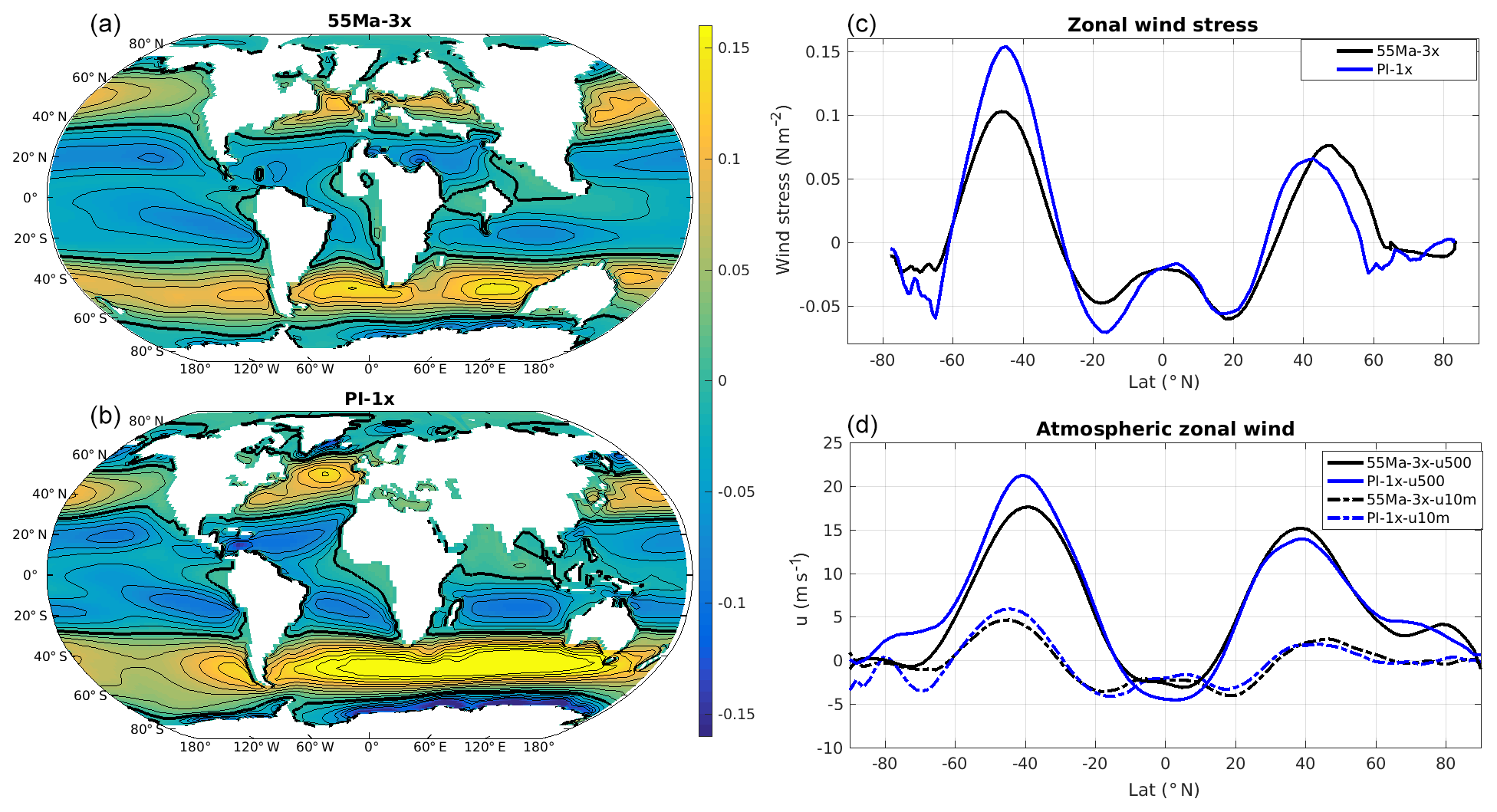
Figure 6Zonal wind stress (N m−2) in the 55 Ma-3x (a) and the PI-1x simulation (b). (c) Zonally averaged zonal wind stress (N m−2) as a function of latitude in the 55 Ma-3x and PI-1x simulations. (d) Zonally averaged zonal wind (m s−1) at 500 hPa in the atmosphere as a function of latitude in the 55 Ma-3x and PI-1x simulations.
In the PI-1x simulation, the maximum intensity of the North Atlantic subtropical and subpolar gyres is respectively 37 and 19 Sv, which is comparable with the intensity of the gyres found in the Southern Hemisphere in the 55 Ma simulations. The most salient feature of the PI-1x simulation is the existence of the Antarctic Circumpolar Current (ACC), with an eastward transport of 108 Sv through the Drake Passage, which totally disrupts the subtropical–subpolar gyre circulation in the different basins of the Southern Hemisphere. In many respects, the South Atlantic and the Weddell Sea during the Eocene are thus an analog of the present-day North Atlantic in terms of the intertwining of subtropical, subpolar and overturning circulation.
4.2 Wind stress
Modern ocean circulation, in particular in the surface layers, is largely driven by surface winds (e.g., Munk, 1950), and it is thus interesting to examine the difference between the PI and 55 Ma horizontal circulation in light of changes in the wind pattern.
Overall, the patterns of wind stress at the ocean surface in the 55 Ma-3x and PI-1x simulations are similar (Fig. 6), although the magnitude differs between the simulations. The sign of this wind stress difference depends on the hemisphere considered. For instance, wind stress is about 30 % weaker in 55 Ma-3x than in PI-1x in the Southern Hemisphere (by 0.05 N m−2 at 45∘ S), whereas it is slightly stronger in the Northern Hemisphere. In the Southern Hemisphere, the difference is particularly striking in the South Atlantic and Indian basins and is largely due to the blocking position of Australia in the early Eocene. The paleogeographic context also explains the increased symmetry in zonal wind stress fields between the Eocene hemispheres relative to the PI.
The more symmetrical pattern of wind stress at the ocean surface in the 55 Ma-3x simulation (compared to PI-1x) is also observed in the zonal wind fields from the surface to 500 hPa in the atmosphere (Fig. 6d). The zonal wind strength is largely determined by the meridional temperature gradient in the atmosphere through the thermal wind relation (Holton and Staley, 1973). Indeed, the meridional temperature gradient in the 55 Ma-3x run (compared to PI-1x) is much reduced in the Southern Hemisphere south of 40∘ S in a large part of the air column (roughly from the surface to at least 500 hPa), in good agreement with the weaker westerly winds found in the 55 Ma-3x run (Fig. 6d). Moreover, the positions of Australia, Africa and South America are located much more southward during the Eocene than the present day, resulting in a blocking effect on zonal winds and reducing the wind stress at 500 hPa by a maximum of 18 % at 40∘ S. In the Northern Hemisphere, the meridional temperature gradient in the 55 Ma-3x simulation is reduced at the surface only north of 60∘ N and similar at 500 hPa relative to the PI-1x, whereas the zonal winds are slightly stronger in the 55 Ma-3x simulation throughout the air column compared to the PI-1x. At the surface, the maximum zonal wind stress is 19 % stronger and shifts poleward by 2∘, mainly due to land–sea distribution.
Changes in ocean gyre circulation between the 55 Ma and PI configurations are mostly due to the large changes in the ocean basin geometry and gateways rather than the moderate changes in the strength and patterns of the wind stress (and its curl). A full understanding of what sets the gyre intensity in the 55 Ma simulations (as well as in the PI simulations) would require further investigations, which are beyond the scope of the present paper.
Modern ocean circulation plays a key role in the regulation of climate through its contribution to the redistribution of heat from the Equator to the poles. In the tropics, the ocean transports roughly 50 % of the 3 PW carried northward by the ocean–atmosphere system but less than 10 % of the total at high latitude (Trenberth and Caron, 2001). The relative contributions of the horizontal and overturning ocean circulations to the meridional heat transport also vary greatly over different latitudes and between oceanic basins (Ganachaud and Wunsch, 2003). In light of the different ocean circulations found in the Eocene and PI conditions, we further investigate in the following how efficient the ocean was at transporting heat across latitudes in the early Eocene.
5.1 Oceanic heat transport
The total meridional OHT at a given latitude y is defined as the sum of advective and diffusive contributions:
where ρ0 is the seawater density, Cp is the specific heat capacity of seawater, v is the meridional velocity, θ is the potential temperature, KH is the horizontal diffusivity coefficient and H is the ocean depth. Here the computation is performed from the model outputs at each model time step. In the early Eocene simulations, there is a significant increase in OHT in the Southern Hemisphere compared to the present-day simulations, but a decrease in the Northern Hemisphere (Fig. 7). As a result, the simulated OHT in the 55 Ma-3x experiment is remarkably asymmetric between hemispheres. The mean OHT difference between the 55 Ma-3x and PI-1x simulations is of the order of 0.2 PW (1 PW =1015 Watt), peaking at 0.5 PW around 35∘ S. The 55 Ma-3x OHT reaches a maximum of 1.7 PW at 15–20∘ S, which is ∼0.3 PW larger than in the present-day simulations at the same latitude but also ∼0.5 PW larger than the maximum PI value of the Northern Hemisphere. This enhanced OHT in the Southern Hemisphere contributes to keeping the Southern Hemisphere particularly warm in the early Eocene, especially south of 50∘ S, as can be seen on the SST distribution (Fig. 2).
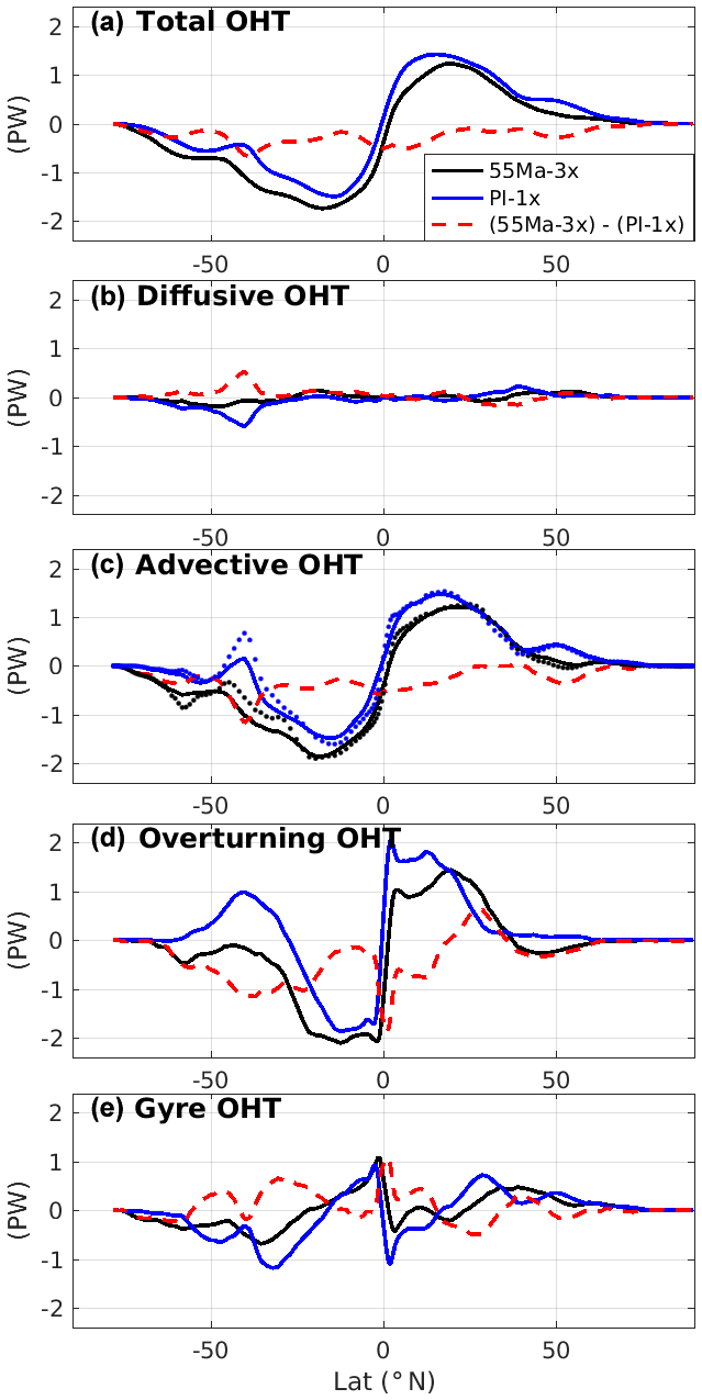
Figure 7Meridional oceanic heat transport (PW) as a function of latitude (positive contribution is northward) and its decomposition according to Eqs. (2) and (3). Results from the 55 Ma-3x and the PI-1x runs are shown in black and blue, respectively, and the difference between the two is in red. In panel (c), the dotted lines indicate the sum of OHTMOC and OHTgyre estimated from monthly means, while the solid lines are computed at the model time step.
Previous studies have examined the role of OHT during the Eocene with a particular focus on the response of the OHT to the opening of Southern Ocean gateways in either realistic Eocene paleogeography or more idealized modern configurations. The OHT simulated by our 55 Ma-3x experiment lies within the range of values found in the literature. For instance, using the NCAR CCSM ocean model with surface heat flux boundary conditions mimicking an energy-balanced atmospheric model, Nong et al. (2000) found that closing the Drake Passage in a modern configuration results in a stronger SOMOC (24 vs. 12 Sv), associated with an increased poleward OHT in the Southern Hemisphere (+0.2 PW, from 1 to 1.2 PW) and a decreased OHT in the Northern Hemisphere. Similarly, using the UVic intermediate-complexity Earth System Climate Model, Sijp and England (2004) found a strongly enhanced heat transport (from 1.6 to 2.4 PW) in the Southern Hemisphere in response to the closure of Drake Passage in a modern configuration. Using the fully coupled NCAR model with a realistic Eocene configuration in which the Drake Passage has a similar configuration to the one we use but the Tasmanian gateway is closed, Huber et al. (2004) performed a set of simulations that exhibited rather weak poleward OHT in the Southern Hemisphere (with a maximum of 0.9 PW at ∼10∘ S), likely because of the absence of a strong SOMOC in their simulations. When closing the Drake Passage in an otherwise modern configuration with the GFDL model, Yang et al. (2014) found that the change in OHT was much larger when the Panama seaway was open, with a strong increase in the OHT in the Southern Hemisphere. More recently, Baatsen et al. (2018) used the higher-resolution CESM Earth system model to simulate the later Eocene (38 Ma) climate, with levels of CO2 and CH4 in the atmosphere prescribed to 2 and 4 times the PI levels. In these two simulations, Baatsen et al. (2018) found a maximum of ∼1.5 PW OHT at 20∘ S in the Southern Hemisphere, associated with a 14–16 Sv SOMOC (compared to the 40 Sv and 1.7 PW at the same latitudes in our 55 Ma-3x simulation).
Although these previous studies are all based on a variety of models with different complexity and resolution, the results consistently suggest that the OHT is largely coupled to the structure and strength of the MOC cells. For instance, the difference in MOC intensity simulated by coupled and uncoupled models could be primarily caused by the positive salt–advection feedback and the self-stabilizing thermal feedback (Sijp and England, 2004). It is noteworthy that the strengthening influence of tidal-induced mixing on the MOC (+7 Sv) is associated with a rather weak increase in OHT, lower than 0.03 PW on average, in agreement with Weber and Thomas (2017). Such a nonlinear relationship between OHT and MOC has also been suggested by Boccaletti (2005), who argued that the shallow circulation locally can be as important as the deep overturning for determining the OHT.
5.2 Decomposition of the meridional ocean heat transport
In order to understand the differences in OHT among our simulations (Fig. 7a), we further split up the OHT into an advective contribution (OHTadv) and a diffusive contribution, corresponding respectively to the first and second term on the right-hand side of Eq. (2) (Fig. 7b and c). This decomposition reveals that, in both the 55 Ma-3x and PI-1x simulations, the advective part dominates the OHT at all latitudes, except at 40∘ S and 40∘ N in PI-1x where the presence of a large temperature gradient (Fig. 2b) results in larger diffusive heat transports. Figure 7b and c also reveal that different OHT between PI-1x and 55 Ma-3x is mainly due to differences in the advective components and the differences in diffusive OHT being rather small.
The advective component, OHTadv, can be decomposed further into an overturning (OHTMOC) and a gyre (OHTgyre) component following, for instance, Bryan (1982) or Volkov et al. (2010):
where and represent the zonal averages of the velocity and temperature, respectively, and v′ and θ′ the deviations from these zonal means. The first term of the right-hand side of Eq. (3) corresponds to the overturning component (OHTMOC), and the second term corresponds to the horizontal transport associated with the large-scale gyre circulation (OHTgyre). Note that due to limitations on the availability of model outputs, the different terms of Eq. (3) presented in Fig. 7d and e are computed from monthly means. This explains why the sum of the two terms does not completely equal OHTadv shown in Fig. 7c, since the latter is computed at each model time step during the simulations. The differences between the two computations can be seen in Fig. 7c.
The decomposition reveals that the enhanced Southern Hemisphere OHTadv in 55 Ma-3x (compared to PI) is overall due to differences in OHTMOC (Fig. 7d, e). The contribution from gyre circulation varies with latitude, with a compensation effect between OHTgyre and OHTMOC in the low latitudes and an enhancement in middle to high latitudes. Consequently, the overall larger OHTadv in the tropics of the 55 Ma-3x simulation is primarily contributed from the strong Eocene OHTMOC (up to 2 PW), which is ∼0.3 PW larger than in the PI simulations. In the midlatitudes of the Southern Hemisphere, where the OHTadv is overall smaller than in the tropics, the OHTMOC in 55 Ma-3x is almost 1 PW stronger than in PI-1x. By contrast, south of 60∘ S, enhanced OHTadv in 55 Ma-3x (compared to PI) results from the combination of stronger OHTgyre and OHTMOC. It is worth noting that OHTgyre at ∼40∘ S in the PI-1x simulation is very likely underestimated in our decomposition computed from monthly mean data because higher-frequency processes (resulting, for instance, from atmospheric synoptic variability) could contribute significantly to OHTgyre in regions where the mean meridional currents are weak (Volkov et al., 2010).
It is obvious from Figs. 3 and 7 that the vigorous SOMOC simulated in the 55 Ma-3x experiment drives a strong net OHT toward the South Pole. This strong SOMOC is associated with the poleward transport of warm waters at shallow depths where zonal oceanic temperature gradients are larger and with a returning equatorward transport of colder water at depth where ocean temperature tends to be more homogenous (Fig. 2c). Remarkably, although the ACC is absent from the Eocene simulation because of different configurations of the Drake and Tasmanian passages that constitute latitudinal barriers (Munday et al., 2015), the contribution of the gyre circulation and diffusive process to poleward heat transport (OHTgyre) is smaller than in the preindustrial simulations. This small OHTgyre in the Eocene simulation is unexpected, given previous hypotheses on the climatic effects of the ACC (e.g., Nong et al., 2000; Toggweiler and Bjornsson, 2000; Sijp and England, 2004). The ACC has indeed been suggested to be a barrier for poleward heat transport so that the onset of the ACC could be a potential driver for the Antarctica-cooling Eocene–Oligocene transition around 34 Ma. However, these studies may not have captured the full complexity of the links between the ACC and OHT in the Southern Ocean. The analysis of both in situ observations (Watts et al., 2016) and the CESM1.0 model (Yang et al., 2015) has indeed revealed that the ACC is composed of meridional excursions of the mean geostrophic horizontal shear flow, energetic eddies and large diffusive heat transport, which balances out equatorward OHT due to Ekman transport and leads to a net poleward OHT in the Southern Ocean (Volkov et al., 2010).
Our analysis has so far focused on the comparison between the 55 Ma-3x and PI-1x simulations, as the former is performed with atmospheric CO2 levels considered to be representative of the early Eocene (Foster et al., 2017; Lunt et al., 2017). The analysis of two additional simulations (55 Ma-1.5x and PI-2x) allows us to investigate the robustness of the ocean circulation in this range of atmospheric CO2 concentrations. These simulations also help us to quantify the sensitivity of the oceanic conditions to a doubling of the CO2 levels in the atmosphere under the early Eocene and modern setting.
The mean ocean temperatures are very sensitive to the atmospheric CO2 concentration in the Eocene configuration (Table 1). The global mean ocean temperature in the Eocene simulations increases by 4.9 ∘C in response to CO2 doubling from 1.5 times to 3 times, which is much larger than the 1 ∘C increase in PI simulations from 1 times to 2 times. The global mean SST in the Eocene also shows a much larger increase as response to a CO2 doubling (+4.7 ∘C) than in the preindustrial (+2.6 ∘C), especially at high latitudes and in the regions of deep convection of the Southern Ocean (Fig. 8), which is similar to the changes in air temperature at 2 m (+5.6 ∘C vs. +3.5 ∘C, respectively; this difference is known as the climate sensitivity). Such contrasting values of climate sensitivity between 55 Ma and PI are in good agreement with the recent results of Farnsworth et al. (2019) obtained with the HadCM3BL model. In the absence of perennial sea ice in 55 Ma simulations, the winter SST in deep convection regions is largely influenced by the air–sea interactions and thus directly related to air temperature, which rarely decreases below 10 ∘C (5 ∘C) in 55 Ma-3x (1.5x) such that the deep waters filling the whole ocean interior vary accordingly with temperature. This is not the case in the present-day configuration wherein deepwater formation is tied to marginal ice zones, such that dense waters formed by brine rejection have initial temperatures close to freezing. Intuitively, we could have expected a larger sensitivity of ocean temperature to atmospheric CO2 in the PI runs because of the ice–albedo feedback. Yet, the effect of this feedback appears to be limited to the high latitudes (Fig. 8) and only plays a marginal role in the changes in global mean SST or the temperatures of the deepwater masses (Table 1).
Table 4Intensity of the gyres (SPGSA: South Atlantic subpolar gyre for 55 Ma; STGNA: North Atlantic subtropical gyre; SPGNA: North Atlantic subpolar gyre; SPGSI: South Indian subpolar gyre; SPGSP: South Pacific subpolar gyre; STGNP: North Pacific subtropical gyre; SPGNP: North Pacific subpolar gyre; ACC: Antarctic Circumpolar Current for PI) and overturning cells (SOMOC: Southern Ocean MOC for 55 Ma; AABW: Antarctic Bottom Water for PI; NADW: North Atlantic Deep Water for PI).
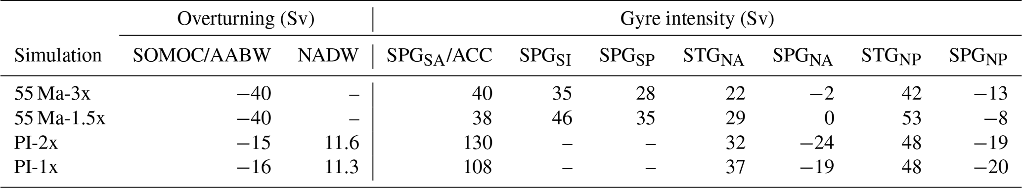
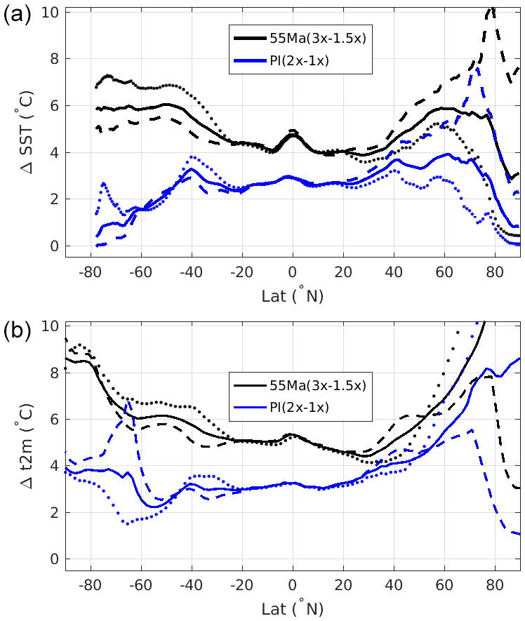
Figure 8Difference of the zonally averaged SST (a, ∘C) and air temperature at 2 m (b, ∘C) as a function of latitude between the 55 Ma-3x and 55 Ma-1.5x runs in black and the PI-2x and PI-1x runs in blue. The solid line indicates the annual mean, the dashed line the mean over July–August–September, and the dotted line the mean over January–February–March.
The ocean circulation exhibits only a minor response to a CO2 doubling in both the Eocene and preindustrial configurations, although this response varies locally (Table 4). In the 55 Ma simulations, the doubling of the CO2 level marginally enhances the maximum abyssal SOMOC (by 0.3 Sv out of 40 Sv in total), while the intensity of the shallow MOC cell and of the barotropic streamfunction is slightly reduced. In the PI simulations, the doubling of atmospheric CO2 levels has the opposite effect on the AABW, whose maximum intensity is reduced by 1.2 Sv (out of ∼15 Sv), whilst the AMOC slightly increases by 0.3 Sv (out of ∼11 Sv). This small increase in the steady-state AMOC is quite interesting and needs to be contrasted with the transient response of the AMOC intensity to global warming (Gent, 2018; Jansen et al., 2018). Indeed, CMIP-type climate models consistently project a strong decline of the AMOC strength when forced with a range of increasing greenhouse gas emission scenarios (Schmittner et al., 2005; Cheng et al., 2013). Yet, when run for longer integrations until full equilibrium, models suggest that the AMOC tends to recover and that the AMOC is ultimately not very sensitive to the CO2 levels (Jansen et al., 2018; Thomas and Fedorov, 2019), as is the case in our PI simulations. Once equilibrium is reached, the most significant effect of a CO2 doubling in our PI experiments is a sharp increase in the ACC transport (+22 Sv out of 108 Sv in PI-1x) in response to stronger westerlies in the Southern Ocean. In contrast, the barotropic circulation remains almost the same in the Pacific but varies in the North Atlantic, with a 5 Sv stronger (weaker) subpolar (subtropical) gyre in the PI-2x simulation compared to PI-1x.
A number of paleoclimate studies have investigated the influence of CO2 levels on ocean circulation in coupled models, with contrasting responses depending on the period considered and the model used. For instance, the deep overturning circulation in the HadCM3L climate model shows an overall high sensitivity to CO2 concentrations in the PETM simulations (Lunt et al., 2010), whilst the GENIE model only exhibits a small response in the Cretaceous simulations of Monteiro et al. (2012). Winguth et al. (2010) further suggest that, in a given simulation of the Paleocene–Eocene period, the different MOC cells (e.g., in the Northern and Southern Hemisphere) could respond differently to a change in CO2 levels. These various responses can be attributed to different factors. First, it is clear that the resolution and overall complexity of the model may partly control the sensitivity of the MOC to CO2 levels, as in models of modern climate (e.g., Bryan et al., 2006). Second, a variety of timescales are intertwined in the adjustment of ocean circulation to external perturbations, from decades for the dynamical adjustment to millennia for the thermodynamical response of bottom waters through vertical advective–diffusive balance (e.g., Donnadieu et al., 2016). The transient response of the ocean can therefore differ from, or even be in the opposite direction of, the final equilibrium response.
The OHT response to a doubling of CO2 in the Eocene simulations is also small, with a slight decrease, in contrast to the OHT increase seen in the PI simulations (although the magnitude of the change is smaller; Fig. 9a). The OHT in the 55 Ma-3x simulation is about 0.15 PW smaller than in the 55 Ma-1.5x simulation over most latitudes. Both overturning and horizontal components contribute to this overall smaller OHT in the 55 Ma-3x simulation (Fig. 9d, e). A weak OHT in the tropics is due to weaker MOC at the same latitudes, while a weak OHT at high latitudes can be attributed to the smaller amplitude of horizontal gyres. In the PI simulations, the OHT in the PI-2x simulation is ∼0.1 PW larger than in PI-1x at high latitudes. This larger OHT in PI-2x is mostly due to the gyre component, which is in good agreement with the ∼5 Sv stronger North Atlantic subpolar gyre and almost no change in the AMOC, for instance.
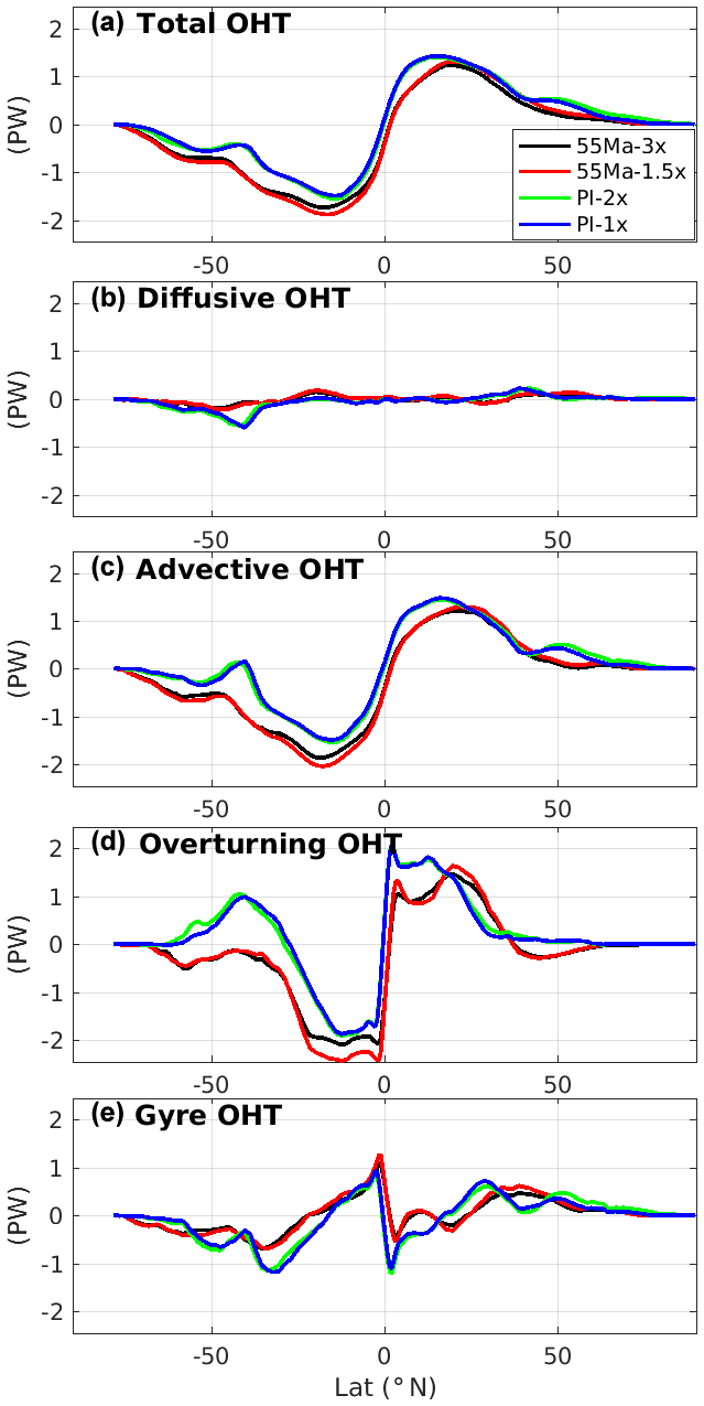
Figure 9Meridional ocean heat transport (PW) as a function of latitude (positive contribution is northward) and its decomposition according to Eqs. (2) and (3) in the four simulations.
Our results therefore support a stable, yet rather small, response of global ocean circulation and heat transport to the doubling of atmospheric CO2 levels. Nevertheless, we have only investigated a limited range of CO2 levels (from 1.5 times to 3 times) and cannot exclude the possibility that the sensitivity of ocean circulation to CO2 concentrations may change at more extreme CO2 levels, as this sensitivity may be highly nonlinear (Lunt et al., 2010). Given that the early Eocene atmosphere CO2 levels are relatively poorly constrained by proxy reconstructions, additional experiments are underway to explore the model response to higher CO2 concentrations in the early Eocene configuration.
Numerous proxy-based reconstructions have revealed that the early Eocene (∼55 Ma) was most likely the warmest period in the Cenozoic. During that period, paleogeographic restrictions of certain modern basins and gateways, such as the North Atlantic and the Drake and Tasmanian passages, suggest fundamental differences from the modern large-scale ocean circulation. It has been proposed that the distinct mode of ocean circulation operating during the early Eocene may have contributed to the significant polar warmth recorded by observational evidence. There is, however, no consensus on the modes of early Eocene ocean circulation or on the relative influence of the overturning and horizontal circulation on the poleward heat transport. Here we revisit this question by analyzing the ocean circulation and its contribution to the meridional OHT using simulations of the early Eocene performed with the IPSL-CM5A2 Earth system model set up with the recent paleogeographic reconstruction of this Eocene time slice distributed as part of the DeepMIP project. Our main results are summarized hereafter.
A strong abyssal overturning circulation (up to 40 Sv) is found in the 55 Ma simulation, with deep water formed only in the Southern Ocean (mainly in the Weddell Sea), whereas there is no deepwater formation in the Northern Hemisphere, in contrast to some previous work on the early Eocene (e.g., Winguth et al., 2012). This situation is favored by orographically induced freshwater fluxes (precipitation and runoff) and maintained by a salt–advection feedback. Indeed, the atmospheric circulation around Antarctica induces relatively low precipitation rates in the Southern Ocean, resulting in higher salinity and hence larger surface density than in the North Pacific, where the orographic precipitation and runoff induced by the presence of the paleo-Rockies tend to reduce surface salinity and inhibit deepwater formation.
The paleogeography (and paleobathymetry) and tidally induced mixing are the main drivers of the strong SOMOC during the early Eocene. The (nearly) closed Drake and Tasmanian passages are of fundamental importance for sustaining the SOMOC via their effect on horizontal ocean circulation. More specifically, with the (nearly) closed Drake and Tasmanian passages serving as a western boundary, clockwise subpolar gyres are well developed (∼40 Sv) in the Weddell and Ross seas, thereby favoring the emergence of deep convection and deepwater formation through isopycnal doming and salt–advection feedback. Tidal-induced mixing also contributes 7 Sv (out of 40 Sv) to this SOMOC, but with only a limited impact on the heat transport.
The vigorous SOMOC simulated for the Eocene is associated with a larger poleward OHT (by a maximum of 0.5 PW relative to PI) in the Southern Hemisphere that largely contributes to maintaining a warm Southern Ocean and Antarctica. Perturbation experiments have been conducted in present-day coupled models to evaluate the impact of an AMOC shutdown. In their model, Vellinga and Wood (2008) found that a 10 Sv reduction in AMOC, associated with a change of its structure, leads to a 1.7 ∘C cooling of the Northern Hemisphere, with a local stronger cooling by 5 ∘C in the northern North Atlantic. This gives credit to the importance of the 40 Sv SOMOC for keeping the Southern Ocean warm in the 55 Ma simulations. Changes in OHT can be compensated for by opposite changes in poleward atmospheric heat transport (ATH), but factors other than a strong SOMOC and associated OHT could contribute to the warm Southern Ocean. Rose and Ferreira (2013) have shown that changes in OHT can induce changes in global mean temperature and meridional temperature gradient through convective adjustment of the extratropical troposphere and increased greenhouse effect. According to their results, the magnitude of those changes could be up to 1 ∘C and 2.6 ∘C for every 0.5 PW enhancement in OHT. Further investigations would be required to examine if this mechanism is also at play in our simulation and whether it contributes significantly to Southern Ocean warmth.
A further decomposition of the OHT reveals that the different overturning circulations between the early Eocene and the preindustrial explain most of the increase in the OHT in the Southern Hemisphere. The contribution of gyre circulation to the OHT is only secondary and varies with latitude, with a compensating effect between the MOC and gyre circulations in the low and midlatitudes, whereas the two contributions add up in the high latitudes. More importantly, the latitudinal distribution of the gyre contribution to the OHT only marginally varies between the early Eocene and preindustrial simulations, despite the absence of the ACC in the early Eocene experiment. Given that the 55 Ma paleobathymetry does not allow for the existence of a strong ACC, this result strongly questions the idea that the ACC could be a strong barrier for OHT in our modern climate and suggests that the meridional excursions of the ACC might indeed play an important role in the gyre-related OHT (Volkov et al., 2010; Watts et al., 2016; Yang et al., 2015).
IPSL-CM5A2 simulation data from this study have been archived in the DeepMIP (https://www.deepmip.org/, DeepMIP, 2020) database and are available by corresponding with Yurui Zhang (yuruizhanglzu@gmail.com).
The supplement related to this article is available online at: https://doi.org/10.5194/cp-16-1263-2020-supplement.
YZ, TH and CL carried out diagnostic analysis with input from YD and JBL. YD and JBL performed the simulations. All authors contributed to the interpretation and discussion of results. YZ wrote the paper with feedback from all authors.
The authors declare that they have no conflict of interest.
We thank the GENCI TGCC at CEA for providing HPC computational resources. We are grateful to Pierre Sepulchre for the initial design of the numerical model. We thank Arnaud Caubel, Anne Cozic, Agnès Ducharne, Josefine Ghattas, François Lott, Olivier Marti, Jean-Yves Peterschmitt and Alistair Sellar for their help in implementing the early Eocene boundary conditions and in resolving technical issues.
This research has received partial funding from the French National Research Agency (ANR) under the “Programme d'Investissements d'Avenir” ISblue (grant no. ANR-17-EURE-0015) and LabexMER (grant no. ANR-10-LABX-19) for the COPS project. Additional funding has been received from Ifremer and the Université Bretagne Loire to support the postdoc of Yurui Zhang. Jean-Baptiste Ladant received funding from the ANR project ANOX-SEA during the early phases of this work.
This paper was edited by Yves Godderis and reviewed by Dan Lunt and one anonymous referee.
Abbott, A. N., Haley, B. A., Tripati, A. K., and Frank, M.: Constraints on ocean circulation at the Paleocene–Eocene Thermal Maximum from neodymium isotopes, Clim. Past, 12, 837–847, https://doi.org/10.5194/cp-12-837-2016, 2016.
Abernathey, R. P., Cerovecki, I., Holland, P. R., Newsom, E., Mazloff, M., and Talley, L. D.: Water-mass transformation by sea ice in the upper branch of the Southern Ocean overturning, Nat. Geosci., 9, 596–601, https://doi.org/10.1038/NGEO2749, 2016.
Anagnostou, E., John, E. H., Edgar, K. M., Foster, G. L., Ridgwell, A., Inglis, G. N., Pancost, R. D., Lunt, D. J., and Pearson, P. N.: Changing atmospheric CO2 concentration was the primary driver of early Cenozoic climate, Nature, 533, 380–384, 2016.
Aumont, O., Ethé, C., Tagliabue, A., Bopp, L., and Gehlen, M.: PISCES-v2: an ocean biogeochemical model for carbon and ecosystem studies, Geosci. Model Dev., 8, 2465–2513, https://doi.org/10.5194/gmd-8-2465-2015, 2015.
Baatsen, M., von der Heydt, A. S., Huber, M., Kliphuis, M. A., Bijl, P. K., Sluijs, A., and Dijkstra, H. A.: Equilibrium state and sensitivity of the simulated middle-to-late Eocene climate, Clim. Past Discuss., https://doi.org/10.5194/cp-2018-43, 2018.
Batenburg, S. J., Voigt, S., Friedrich, O., Osborne, A. H., Bornemann, A., Klein, T., Pérez-Díaz, L., and Frank, M.: Major intensification of Atlantic overturning circulation at the onset of Paleogene greenhouse warmth, Nat. Commun., 9, 4954, https://doi.org/10.1038/s41467-018-07457-7, 2018.
Boccaletti, G.: The vertical structure of ocean heat transport, Geophys. Res. Lett., 32, L10603, https://doi.org/10.1029/2005GL022474, 2005.
Boyer, T., Levitus, S., Garcia, H., Locarnini, R. A., Stephens, C., and Antonov, J.: Objective analyses of annual, seasonal, and monthly temperature and salinity for the World Ocean on a 0.25∘ grid, Int. J. Climatol., 25, 931–945, https://doi.org/10.1002/joc.1173, 2005.
Bryan, F.: Parameter Sensitivity of Primitive Equation Ocean General Circulation Models, J. Phys. Oceanogr., 17, 970–985, https://doi.org/10.1175/1520-0485(1987)017<0970:PSOPEO>2.0.CO;2, 1987.
Bryan, F. O., Danabasoglu, G., Nakashiki, N., Yoshida, Y., Kim, D.-H., Tsutsui, J., and Doney, S. C.: Response of the North Atlantic Thermohaline Circulation and Ventilation to Increasing Carbon Dioxide in CCSM3, J. Climate, 19, 2382–2397, https://doi.org/10.1175/JCLI3757.1, 2006.
Bryan, K.: Poleward Heat Transport by the Ocean: Observations and Models, Annu. Rev. Earth Pl. Sc., 10, 15–38, https://doi.org/10.1146/annurev.ea.10.050182.000311, 1982.
Carmichael, M. J., Lunt, D. J., Huber, M., Heinemann, M., Kiehl, J., LeGrande, A., Loptson, C. A., Roberts, C. D., Sagoo, N., Shields, C., Valdes, P. J., Winguth, A., Winguth, C., and Pancost, R. D.: A model–model and data–model comparison for the early Eocene hydrological cycle, Clim. Past, 12, 455–481, https://doi.org/10.5194/cp-12-455-2016, 2016.
Cheng, W., Chiang, J. C. H., and Zhang, D.: Atlantic Meridional Overturning Circulation (AMOC) in CMIP5 Models: RCP and Historical Simulations, J. Climate, 26, 7187–7197, https://doi.org/10.1175/JCLI-D-12-00496.1, 2013.
Cramer, B. S., Miller, K. G., Barrett, P. J., and Wright, J. D.: Late Cretaceous–Neogene trends in deep ocean temperature and continental ice volume: Reconciling records of benthic foraminiferal geochemistry (δ18O and Mg∕Ca) with sea level history, J. Geophys. Res., 116, C12023, https://doi.org/10.1029/2011JC007255, 2011.
de Boer, A. M., Sigman, D. M., Toggweiler, J. R., and Russell, J. L.: Effect of global ocean temperature change on deep ocean ventilation, Paleoceanography, 22, PA2210, https://doi.org/10.1029/2005PA001242, 2007.
DeepMIP: The Deep-Time Model Intercomparison Project, available at: https://www.deepmip.org/, last access: 13 July 2020.
de Lavergne, C., Madec, G., Le Sommer, J., Nurser, A. J. G., and Naveira Garabato, A. C.: On the Consumption of Antarctic Bottom Water in the Abyssal Ocean, J. Phys. Oceanogr., 46, 635–661, https://doi.org/10.1175/JPO-D-14-0201.1, 2016.
de Lavergne, C., Falahat, S., Madec, G., Roquet, F., Nycander, J., and Vic, C.: Toward global maps of internal tide energy sinks, Ocean Model., 137, 52–75, https://doi.org/10.1016/j.ocemod.2019.03.010, 2019.
Donnadieu, Y., Pucéat, E., Moiroud, M., Guillocheau, F., and Deconinck, J.-F.: A better-ventilated ocean triggered by Late Cretaceous changes in continental configuration, Nat. Commun., 7, 10316, https://doi.org/10.1038/ncomms10316, 2016.
Drijfhout, S. S. and Hazeleger, W.: Changes in MOC and gyre-induced Atlantic Ocean heat transport, Geophys. Res. Lett., 33, L07707, https://doi.org/10.1029/2006GL025807, 2006.
Dunkley Jones, T., Lunt, D. J., Schmidt, D. N., Ridgwell, A., Sluijs, A., Valdes, P. J., and Maslin, M.: Climate model and proxy data constraints on ocean warming across the Paleocene–Eocene Thermal Maximum, Earth-Sci. Rev., 125, 123–145, https://doi.org/10.1016/j.earscirev.2013.07.004, 2013.
Emile-Geay, J. and Madec, G.: Geothermal heating, diapycnal mixing and the abyssal circulation, Ocean Sci., 5, 203–217, https://doi.org/10.5194/os-5-203-2009, 2009.
England, M. H., Hutchinson, D. K., Santoso, A., and Sijp, W. P.: Ice–Atmosphere Feedbacks Dominate the Response of the Climate System to Drake Passage Closure, J. Climate, 30, 5775–5790, https://doi.org/10.1175/JCLI-D-15-0554.1, 2017.
Evans, D., Sagoo, N., Renema, W., Cotton, L. J., Müller, W., Todd, J. A., Saraswati, P. K., Stassen, P., Ziegler, M., Pearson, P. N., Valdes, P. J., and Affek, H. P.: Eocene greenhouse climate revealed by coupled clumped isotope-Mg∕Ca thermometry, P. Natl. Acad. Sci. USA, 115, 1174–1179, https://doi.org/10.1073/pnas.1714744115, 2018.
Farnsworth, A., Lunt, D. J., O'Brien, C. L., Foster, G. L., Inglis, G. N., Markwick, P., Pancost, R. D., and Robinson, S. A.: Climate Sensitivity on Geological Timescales Controlled by Nonlinear Feedbacks and Ocean Circulation, Geophys. Res. Lett., 46, 9880–9889, https://doi.org/10.1029/2019GL083574, 2019.
Ferreira, D., Cessi, P., Coxall, H. K., de Boer, A., Dijkstra, H. A., Drijfhout, S. S., Eldevik, T., Harnik, N., McManus, J. F., Marshall, D. P., Nilsson, J., Roquet, F., Schneider, T., and Wills, R. C.: Atlantic-Pacific Asymmetry in Deep Water Formation, Annu. Rev. Earth Pl. Sc., 46, 327–352, https://doi.org/10.1146/annurev-earth-082517-010045, 2018.
Fichefet, T. and Maqueda, M. A. M.: Sensitivity of a global sea ice model to the treatment of ice thermodynamics and dynamics, J. Geophys. Res., 102, 12609–12646, https://doi.org/10.1029/97JC00480, 1997.
Foster, G. L., Royer, D. L., and Lunt, D. J.: Future climate forcing potentially without precedent in the last 420 million years, Nat. Commun., 8, 14845, https://doi.org/10.1038/ncomms14845, 2017.
Frank, M.: Radiogenic isotopes: Tracers of past ocean circulation and erosional input, Rev. Geophys., 40, 1001, https://doi.org/10.1029/2000RG000094, 2002.
Galeotti, S., DeConto, R., Naish, T., Stocchi, P., Florindo, F., Pagani, M., Barrett, P., Bohaty, S. M., Lanci, L., Pollard, D., Sandroni, S., Talarico, F. M., and Zachos, J. C.: Antarctic Ice Sheet variability across the Eocene-Oligocene boundary climate transition, Science, 352, 76–80, https://doi.org/10.1126/science.aab0669, 2016.
Ganachaud, A. and Wunsch, C.: Large-Scale Ocean Heat and Freshwater Transports during the World Ocean Circulation Experiment, J. Climate, 16, 696–705, 2003.
Gasson, E., Lunt, D. J., DeConto, R., Goldner, A., Heinemann, M., Huber, M., LeGrande, A. N., Pollard, D., Sagoo, N., Siddall, M., Winguth, A., and Valdes, P. J.: Uncertainties in the modelled CO2 threshold for Antarctic glaciation, Clim. Past, 10, 451–466, https://doi.org/10.5194/cp-10-451-2014, 2014.
Gent, P. R.: A commentary on the Atlantic meridional overturning circulation stability in climate models, Ocean Model., 122, 57–66, https://doi.org/10.1016/j.ocemod.2017.12.006, 2018.
Green, J. A. M. and Huber, M.: Tidal dissipation in the early Eocene and implications for ocean mixing: EOCENE TIDES, Geophys. Res. Lett., 40, 2707–2713, https://doi.org/10.1002/grl.50510, 2013.
Herold, N., Buzan, J., Seton, M., Goldner, A., Green, J. A. M., Müller, R. D., Markwick, P., and Huber, M.: A suite of early Eocene (∼55 Ma) climate model boundary conditions, Geosci. Model Dev., 7, 2077–2090, https://doi.org/10.5194/gmd-7-2077-2014, 2014.
Heuzé, C., Heywood, K. J., Stevens, D. P., and Ridley, J. K.: Changes in Global Ocean Bottom Properties and Volume Transports in CMIP5 Models under Climate Change Scenarios, J. Climate, 28, 2917–2944, https://doi.org/10.1175/JCLI-D-14-00381.1, 2015.
Hollis, C. J., Dunkley Jones, T., Anagnostou, E., Bijl, P. K., Cramwinckel, M. J., Cui, Y., Dickens, G. R., Edgar, K. M., Eley, Y., Evans, D., Foster, G. L., Frieling, J., Inglis, G. N., Kennedy, E. M., Kozdon, R., Lauretano, V., Lear, C. H., Littler, K., Lourens, L., Meckler, A. N., Naafs, B. D. A., Pälike, H., Pancost, R. D., Pearson, P. N., Röhl, U., Royer, D. L., Salzmann, U., Schubert, B. A., Seebeck, H., Sluijs, A., Speijer, R. P., Stassen, P., Tierney, J., Tripati, A., Wade, B., Westerhold, T., Witkowski, C., Zachos, J. C., Zhang, Y. G., Huber, M., and Lunt, D. J.: The DeepMIP contribution to PMIP4: methodologies for selection, compilation and analysis of latest Paleocene and early Eocene climate proxy data, incorporating version 0.1 of the DeepMIP database, Geosci. Model Dev., 12, 3149–3206, https://doi.org/10.5194/gmd-12-3149-2019, 2019.
Holton, J. R. and Staley, D. O.: An Introduction to Dynamic Meteorology, Am. J. Phys., 41, 752–754, https://doi.org/10.1119/1.1987371, 1973.
Hourdin, F., Grandpeix, J.-Y., Rio, C., Bony, S., Jam, A., Cheruy, F., Rochetin, N., Fairhead, L., Idelkadi, A., Musat, I., Dufresne, J.-L., Lahellec, A., Lefebvre, M.-P., and Roehrig, R.: LMDZ5B: the atmospheric component of the IPSL climate model with revisited parameterizations for clouds and convection, Clim. Dynam., 40, 2193–2222, https://doi.org/10.1007/s00382-012-1343-y, 2013.
Huber, B. T., Macleod, K. G., and Wing, S. L.: Warm Climates in Earth History, Cambridge University Press, 2000.
Huber, M.: Progress in Greenhouse Climate Modelling, The Paleontological Society Papers, 18, 213–262, 2012.
Huber, M. and Caballero, R.: The early Eocene equable climate problem revisited, Clim. Past, 7, 603–633, https://doi.org/10.5194/cp-7-603-2011, 2011.
Huber, M., Brinkhuis, H., Stickley, C. E., Döös, K., Sluijs, A., Warnaar, J., Schellenberg, S. A., and Williams, G. L.: Eocene circulation of the Southern Ocean: Was Antarctica kept warm by subtropical waters?, Paleoceanography, 19, 4026, https://doi.org/10.1029/2004PA001014, 2004.
Hutchinson, D. K., de Boer, A. M., Coxall, H. K., Caballero, R., Nilsson, J., and Baatsen, M.: Climate sensitivity and meridional overturning circulation in the late Eocene using GFDL CM2.1, Clim. Past, 14, 789–810, https://doi.org/10.5194/cp-14-789-2018, 2018.
Jansen, M. F., Nadeau, L.-P., and Merlis, T. M.: Transient versus Equilibrium Response of the Ocean's Overturning Circulation to Warming, J. Climate, 31, 5147–5163, https://doi.org/10.1175/JCLI-D-17-0797.1, 2018.
Kageyama, M., Braconnot, P., Bopp, L., Caubel, A., Foujols, M.-A., Guilyardi, E., Khodri, M., Lloyd, J., Lombard, F., Mariotti, V., Marti, O., Roy, T., and Woillez, M.-N.: Mid-Holocene and Last Glacial Maximum climate simulations with the IPSL model–part I: comparing IPSL_CM5A to IPSL_CM4, Clim. Dynam., 40, 2447–2468, https://doi.org/10.1007/s00382-012-1488-8, 2013.
Koch-Larrouy, A., Madec, G., Bouruet-Aubertot, P., Gerkema, T., Bessières, L., and Molcard, R.: On the transformation of Pacific Water into Indonesian Throughflow Water by internal tidal mixing, Geophys. Res. Lett., 34, L04604, https://doi.org/10.1029/2006GL028405, 2007.
Krinner, G., Viovy, N., de Noblet-Ducoudré, N., Ogée, J., Polcher, J., Friedlingstein, P., Ciais, P., Sitch, S., and Prentice, I. C.: A dynamic global vegetation model for studies of the coupled atmosphere-biosphere system, Global Biogeochem. Cy., 19, GB1015, https://doi.org/10.1029/2003GB002199, 2005.
Ladant, J.-B., Donnadieu, Y., Lefebvre, V., and Dumas, C.: The respective role of atmospheric carbon dioxide and orbital parameters on ice sheet evolution at the Eocene-Oligocene transition: Ice sheet evolution at the EOT, Paleoceanography, 29, 810–823, https://doi.org/10.1002/2013PA002593, 2014.
Ladant, J.-B., Donnadieu, Y., Bopp, L., Lear, C. H., and Wilson, P. A.: Meridional Contrasts in Productivity Changes Driven by the Opening of Drake Passage, Paleoceanogr. Paleocl., 33, 302–317, https://doi.org/10.1002/2017PA003211, 2018.
Lott, F. and Miller, M. J.: A new subgrid-scale orographic drag parametrization: Its formulation and testing, Q. J. Roy. Meteor. Soc., 123, 101–127, 1997.
Lott, F. O.: Alleviation of Stationary Biases in a GCM through a Mountain Drag Parameterization Scheme and a Simple Representation of Mountain Lift Forces, Mon. Weather Rev., 127, 778–801, 1999.
Lumpkin, R. and Speer, K.: Global Ocean Meridional Overturning, J. Phys. Oceanogr., 37, 2550–2562, https://doi.org/10.1175/JPO3130.1, 2007.
Lunt, D. J., Valdes, P. J., Jones, T. D., Ridgwell, A., Haywood, A. M., Schmidt, D. N., Marsh, R., and Maslin, M.: CO2-driven ocean circulation changes as an amplifier of Paleocene-Eocene thermal maximum hydrate destabilization, Geology, 38, 875–878, https://doi.org/10.1130/G31184.1, 2010.
Lunt, D. J., Huber, M., Anagnostou, E., Baatsen, M. L. J., Caballero, R., DeConto, R., Dijkstra, H. A., Donnadieu, Y., Evans, D., Feng, R., Foster, G. L., Gasson, E., von der Heydt, A. S., Hollis, C. J., Inglis, G. N., Jones, S. M., Kiehl, J., Kirtland Turner, S., Korty, R. L., Kozdon, R., Krishnan, S., Ladant, J.-B., Langebroek, P., Lear, C. H., LeGrande, A. N., Littler, K., Markwick, P., Otto-Bliesner, B., Pearson, P., Poulsen, C. J., Salzmann, U., Shields, C., Snell, K., Stärz, M., Super, J., Tabor, C., Tierney, J. E., Tourte, G. J. L., Tripati, A., Upchurch, G. R., Wade, B. S., Wing, S. L., Winguth, A. M. E., Wright, N. M., Zachos, J. C., and Zeebe, R. E.: The DeepMIP contribution to PMIP4: experimental design for model simulations of the EECO, PETM, and pre-PETM (version 1.0), Geosci. Model Dev., 10, 889–901, https://doi.org/10.5194/gmd-10-889-2017, 2017.
Madec, G. and the NEMO team: NEMO ocean engine, available at: https://www.nemo-ocean.eu/wp-content/uploads/NEMO_book.pdf (last access: 13 July 2020), 2016.
Maffre, P., Ladant, J.-B., Donnadieu, Y., Sepulchre, P., and Goddéris, Y.: The influence of orography on modern ocean circulation, Clim. Dynam., 50, 1277–1289, https://doi.org/10.1007/s00382-017-3683-0, 2018.
Manabe, S. and Stouffer, R. J.: The role of thermohaline circulation in climate, Tellus B, 51, 91–109, https://doi.org/10.1034/j.1600-0889.1999.00008.x, 1999.
Marshall, J. and Schott, F.: Open-ocean convection: Observations, theory, and models, Rev. Geophys., 37, 1–64, https://doi.org/10.1029/98RG02739, 1999.
Marshall, J. and Speer, K.: Closure of the meridional overturning circulation through Southern Ocean upwelling, Nat. Geosci., 5, 171–180, 2012.
McCarthy, G. D., Smeed, D. A., Johns, W. E., Frajka-Williams, E., Moat, B. I., Rayner, D., Baringer, M. O., Meinen, C. S., Collins, J., and Bryden, H. L.: Measuring the Atlantic Meridional Overturning Circulation at 26∘ N, Prog. Oceanogr., 130, 91–111, https://doi.org/10.1016/j.pocean.2014.10.006, 2015.
Monteiro, F. M., Pancost, R. D., Ridgwell, A., and Donnadieu, Y.: Nutrients as the dominant control on the spread of anoxia and euxinia across the Cenomanian-Turonian oceanic anoxic event (OAE2): Model-data comparison, Paleoceanography, 27, PA4209, https://doi.org/10.1029/2012PA002351, 2012.
Msadek, R., Johns, W. E., Yeager, S. G., Danabasoglu, G., Delworth, T. L., and Rosati, A.: The Atlantic Meridional Heat Transport at 26.5∘ N and Its Relationship with the MOC in the RAPID Array and the GFDL and NCAR Coupled Models, J. Climate, 26, 4335–4356, https://doi.org/10.1175/JCLI-D-12-00081.1, 2013.
Müller, R. D., Sdrolias, M., Gaina, C., and Roest, W. R.: Age, spreading rates, and spreading asymmetry of the world's ocean crust, Geochem. Geophy. Geosy., 9, Q04006, https://doi.org/10.1029/2007GC001743, 2008.
Munday, D. R., Johnson, H. L., and Marshall, D. P.: The role of ocean gateways in the dynamics and sensitivity to wind stress of the early Antarctic Circumpolar Current, Paleoceanography, 30, 284–302, https://doi.org/10.1002/2014PA002675, 2015.
Munk, W. H.: On the wind-driven ocean circulation, J. Meteorol., 7, 79–93, https://doi.org/10.1175/1520-0469(1950)007<0080:OTWDOC>2.0.CO;2, 1950.
Nikurashin, M. and Ferrari, R.: Overturning circulation driven by breaking internal waves in the deep ocean, Geophys. Res. Lett., 40, 3133–3137, https://doi.org/10.1002/grl.50542, 2013.
Nong, G. T., Najjar, R. G., Seidov, D., and Peterson, W. H.: Simulation of ocean temperature change due to the opening of Drake Passage, Geophys. Res. Lett., 27, 2689–2692, https://doi.org/10.1029/1999GL011072, 2000.
Rose, B. E. J. and Ferreira, D.: Ocean Heat Transport and Water Vapor Greenhouse in a Warm Equable Climate: A New Look at the Low Gradient Paradox, J. Climate, 26, 2117–2136, https://doi.org/10.1175/JCLI-D-11-00547.1, 2013.
Schmittner, A., Latif, M., and Schneider, B.: Model projections of the North Atlantic thermohaline circulation for the 21st century assessed by observations, Geophys. Res. Lett., 32, L23710, https://doi.org/10.1029/2005GL024368, 2005.
Sepulchre, P., Caubel, A., Ladant, J.-B., Bopp, L., Boucher, O., Braconnot, P., Brockmann, P., Cozic, A., Donnadieu, Y., Dufresne, J.-L., Estella-Perez, V., Ethé, C., Fluteau, F., Foujols, M.-A., Gastineau, G., Ghattas, J., Hauglustaine, D., Hourdin, F., Kageyama, M., Khodri, M., Marti, O., Meurdesoif, Y., Mignot, J., Sarr, A.-C., Servonnat, J., Swingedouw, D., Szopa, S., and Tardif, D.: IPSL-CM5A2 – an Earth system model designed for multi-millennial climate simulations, Geosci. Model Dev., 13, 3011–3053, https://doi.org/10.5194/gmd-13-3011-2020, 2020.
Sijp, W. P. and England, M. H.: Effect of the Drake Passage Throughflow on Global Climate, J. Phys. Oceanogr., 34, 1254–1266, 2004.
Sijp, W. P., von der Heydt, A. S., Dijkstra, H. A., Flögel, S., Douglas, P. M. J., and Bijl, P. K.: The role of ocean gateways on cooling climate on long time scales, Global Planet. Change, 119, 1–22, https://doi.org/10.1016/j.gloplacha.2014.04.004, 2014.
Simmons, H. L., Jayne, S. R., Laurent, L. C. S., and Weaver, A. J.: Tidally driven mixing in a numerical model of the ocean general circulation, Ocean Model., 6, 245–263, https://doi.org/10.1016/S1463-5003(03)00011-8, 2004.
St. Laurent, L. C., Simmons, H. L., and Jayne, S. R.: Estimating tidally driven mixing in the deep ocean, Geophys. Res. Lett., 29, 2106, https://doi.org/10.1029/2002GL015633, 2002.
Stein, C. A. and Stein, S.: A model for the global variation in oceanic depth and heat flow with lithospheric age, Nature, 359, 123–129, https://doi.org/10.1038/359123a0, 1992.
Thomas, D. J., Bralower, T. J., and Jones, C. E.: Neodymium isotopic reconstruction of late Paleocene–early Eocene thermohaline circulation, Earth Planet. Sc. Lett., 209, 309–322, https://doi.org/10.1016/S0012-821X(03)00096-7, 2003.
Thomas, D. J., Korty, R., Huber, M., Schubert, J. A., and Haines, B.: Nd isotopic structure of the Pacific Ocean 70-30 Ma and numerical evidence for vigorous ocean circulation and ocean heat transport in a greenhouse world, Paleoceanography, 29, 454–469, https://doi.org/10.1002/2013PA002535, 2014.
Thomas, M. D. and Fedorov, A. V.: Mechanisms and Impacts of a Partial AMOC Recovery Under Enhanced Freshwater Forcing, Geophys. Res. Lett., 46, 3308–3316, https://doi.org/10.1029/2018GL080442, 2019.
Toggweiler, J. R. and Bjornsson, H.: Drake Passage and palaeoclimate, J. Quaternary Sci., 15, 319–328, 2000.
Trenberth, K. E. and Caron, J. M.: Estimates of Meridional Atmosphere and Ocean Heat Transports, J. Climate, 14, 3433–3443, 2001.
Vellinga, M. and Wood, R. A.: Impacts of thermohaline circulation shutdown in the twenty-first century, Climatic Change, 91, 43–63, https://doi.org/10.1007/s10584-006-9146-y, 2008.
Voigt, S., Jung, C., Friedrich, O., Frank, M., Teschner, C., and Hoffmann, J.: Tectonically restricted deep-ocean circulation at the end of the Cretaceous greenhouse, Earth Planet. Sc. Lett., 369–370, 169–177, https://doi.org/10.1016/j.epsl.2013.03.019, 2013.
Volkov, D. L., Fu, L.-L., and Lee, T.: Mechanisms of the meridional heat transport in the Southern Ocean, Clim. Dynam., 60, 791–801, https://doi.org/10.1007/s10236-010-0288-0, 2010.
Watts, D. R., Tracey, K. L., Donohue, K. A., and Chereskin, T. K.: Estimates of Eddy Heat Flux Crossing the Antarctic Circumpolar Current from Observations in Drake Passage, J. Phys. Oceanogr., 46, 2103–2122, https://doi.org/10.1175/JPO-D-16-0029.1, 2016.
Weber, T. and Thomas, M.: Influence of ocean tides on the general ocean circulation in the early Eocene, Paleoceanography, 32, 553–570, https://doi.org/10.1002/2016PA002997, 2017.
Winguth, A., Shellito, C., Shields, C., and Winguth, C.: Climate Response at the Paleocene–Eocene Thermal Maximum to Greenhouse Gas Forcing–A Model Study with CCSM3, J. Climate, 23, 2562–2584, https://doi.org/10.1175/2009JCLI3113.1, 2010.
Winguth, A. M. E., Thomas, E., and Winguth, C.: Global decline in ocean ventilation, oxygenation, and productivity during the Paleocene-Eocene Thermal Maximum: Implications for the benthic extinction, Geology, 40, 263–266, https://doi.org/10.1130/G32529.1, 2012.
Wolfe, C. L. and Cessi, P.: Salt Feedback in the Adiabatic Overturning Circulation, J. Phys. Oceanogr., 44, 1175–1194, https://doi.org/10.1175/JPO-D-13-0154.1, 2014.
Yang, H., Wang, Y., and Liu, Z.: A modelling study of the Bjerknes compensation in the meridional heat transport in a freshening ocean, Tellus A, 65, 18480, https://doi.org/10.3402/tellusa.v65i0.18480, 2013.
Yang, H., Li, Q., Wang, K., Sun, Y., and Sun, D.: Decomposing the meridional heat transport in the climate system, Clim. Dynam., 44, 2751–2768, https://doi.org/10.1007/s00382-014-2380-5, 2015.
Yang, S., Galbraith, E., and Palter, J.: Coupled climate impacts of the Drake Passage and the Panama Seaway, Clim. Dynam., 43, 37–52, https://doi.org/10.1007/s00382-013-1809-6, 2014.
Zachos, J. C, Pagani, M., Sloan, L., Thomas, E., and Billups, K: Trends, Rhythms, and Aberrations in Global Climate 65 Ma to Present, Science, 292, 686–693, https://doi.org/10.1126/science.1059412, 2001.
Zachos, J. C., Dickens, G. R., and Zeebe, R. E.: An early Cenozoic perspective on greenhouse warming and carbon-cycle dynamics, Nature, 451, 279–283, https://doi.org/10.1038/nature06588, 2008.
Zeebe, R. E. and Zachos, J. C.: Reversed deep-sea carbonate ion basin gradient during Paleocene-Eocene thermal maximum, Paleoceanography, 22, PA3201, https://doi.org/10.1029/2006PA001395, 2007.
Zhang, R.: Latitudinal dependence of Atlantic meridional overturning circulation (AMOC) variations, Geophys. Res. Lett., 37, 76–84, https://doi.org/10.1029/2010GL044474, 2010.
- Abstract
- Introduction
- Numerical model data
- The overturning circulation
- Horizontal circulation and winds
- Oceanic heat transport and its decomposition
- Sensitivity of the ocean response to a doubling of the levels of atmospheric CO2
- Conclusions
- Data availability
- Author contributions
- Competing interests
- Acknowledgements
- Financial support
- Review statement
- References
- Supplement