Inconsistencies between observed, reconstructed, and simulated precipitation indices for England since the year 1650 CE

The scarcity of long instrumental records, uncertainty in reconstructions, and insufficient skill in model simulations hamper assessing how regional precipitation changed over past centuries. Here, we use standardized precipitation data to compare a regional climate simulation, reconstructions, and long observational records of seasonal (March to July) mean precipitation in England and Wales over the past 350 years. The Standardized Precipitation Index is a valuable tool for assessing agreement between the different sources of information, as it allows for a comparison of the temporal evolution of percentiles of the precipitation distributions. These evolutions are not consistent among reconstructions, a regional simulation, and instrumental observations for severe and extreme dry and wet conditions. The lack of consistency between the different data sets may be due to the dominance of internal climate variability over the impact of natural exogenous forcing conditions on multi-decadal timescales. The disagreement between sources of information reduces our confidence in inferences about the origins of hydroclimate variability for small regions. However, it is encouraging that there is still some agreement between a regional simulation and observations. Our results emphasize the complexity of hydroclimate changes during the recent centuries and stress the necessity of a thorough understanding of the processes affecting forced and unforced precipitation variability.

1 Introduction

Confidence in future climate projections of, e.g., drought and wetness conditions requires an understanding of past climate and hydroclimate variability and its drivers (e.g., Schmidt et al., 2014). Focusing on the hydroclimate, estimates of past and future changes are still highly uncertain for precipitation at regional scales. Indeed, our understanding of internal, naturally forced, and anthropogenically forced variability is weaker for precipitation than for temperature due to the more complex controls on precipitation variability (e.g., Zhang et al., 2007; Hoerling et al., 2009; Iles et al., 2013; Fischer et al., 2014) and the more local-scale nature of precipitation processes.

Consistency among estimates from early instrumental observations, paleo-reconstructions from environmental archives (i.e., paleo-observations), and climate simulations supports our understanding of past changes. It strengthens our confidence in inferences if the sources of information prove to be consistent. Here, consistency among estimates simply means that various sources of information do not contradict each other. Despite being a rather liberal metric, consistency is an appropriate measure in view of the multiple sources of uncertainty in inferring past hydroclimate and precipitation variability.

Here, we explore the consistency of observations, reconstructions, and simulations for one small region and focus only on precipitation changes. Specifically, we set out to study the consistency in the statistical properties of precipitation distributions in these sources of information.

Comparing precipitation among different data sources poses various challenges. Problems relate but are not limited to pronounced biases in the simulated precipitation, especially derived from raw global models, and to differences in representation or, in the case of fields of data, the spatial resolution. In the context of long observational time series, data inhomogeneities due to changes in instrumentation, measuring techniques, and changes in locations can further influence estimates of longer-term trends (e.g., Frank et al., 2007; Wilson et al., 2005; Böhm et al., 2010; Burt and Howden, 2011; Craddock and Craddock, 1977). Reconstructions likely represent only part of the variability spectrum of, e.g., precipitation, dependent on the strength of the climatic signal in the original data and on further shortcomings of the underlying paleo-observations.

The PAGES Hydro2k Consortium (2017) discuss in more detail the problems in comparing hydroclimatic variables between reconstructions and simulations. They developed recommendations for the comparison of hydroclimate representations in simulations and paleo-observations. They stress the complementary nature of simulated and environmental information considering their respective uncertainties. Estimates have to represent the same parameters on related spatial and temporal scales. Only then can a comparison be valid. We need appropriate methods to bridge the gap between the local or regional reconstruction and the simulation output that represents aggregates over larger spatial scales. Proxy system models are one means to achieve this (Evans et al., 2013; PAGES Hydro2k Consortium, 2017).

Transforming precipitation estimates to the Standardized Precipitation Index (SPI; McKee et al., 1993) facilitates the comparison of different sources of information on precipitation in view of the mentioned challenges. It provides a common basis for comparisons between different locations, periods, or seasons. The core of the SPI calculation is the fit of a distribution function to the precipitation estimates. We argue that the transformation of precipitation estimates to the SPI is a simple means to compare the statistical properties of hydroclimatic parameters in simulations and paleo-observations. It is of value for periods with and without comprehensive sets of climate and weather observations.

Previous usage of the SPI in paleoclimatology focused on the index series (compare, e.g., Domínguez-Castro et al., 2008; Seftigen et al., 2013) and did not consider further information available through the transformation. We apply the SPI over moving windows of 51 years to study variations in the properties of precipitation distributions on multi-decadal timescales. We concentrate on a regional domain where all sources of data, i.e., observations, reconstructions, and simulations, are available. By applying the SPI transformation over moving windows, we are able to evaluate and compare percentiles of the estimates as well as the moments of the distributions and the temporal changes in these distributional properties. We are essentially comparing sequences of climatologies.

Long observationally based records allow us to assess how the statistics of observed precipitation have changed over the last couple of centuries. They, in turn, provide the basis for evaluating how state-of-the art regional or global climate model simulations and reconstructions for the Common Era (CE) compare in domains colocated with the available observations. We choose southern Great Britain as our domain of interest since there are precipitation observations available in the form of the England–Wales precipitation data set (Alexander and Jones, 2000, for the period 1766 CE to present), its subdivisions, and instrumental records for Oxford (cf. Radcliffe), Pode Hole, and Kew Gardens. The instrumental records start in 1767, 1726, and 1697 CE, respectively.

A number of precipitation reconstructions are available for southern Great Britain. We choose the millennium-long tree-ring-based data by Cooper et al. (2013) and Wilson et al. (2013) for East Anglia and southern–central England, respectively. We focus on an extended spring season (MAMJJ). The next section discusses our decision to concentrate on these data instead of the δ¹⁸O-based scaling approaches by Young et al. (2015, covering the period 1766 to present) and Rinne et al. (2013, reconstructed values from 1613 to 1893 CE).

Regional simulations for the last 500 to 2000 years are rare. To our knowledge there are only two transient regional simulations. Gómez-Navarro et al. (2015) compare one of these simulations, with the model MM5, to reconstructions for various parameters over larger regional domains within Europe. For precipitation, they compare the simulation to the gridded precipitation reconstructions of Pauling et al. (2006) for western Europe, which is based on a set of dendroclimatological and other natural proxies and documentary information. Gómez-Navarro et al. (2015) find rather good agreement in the evolution of median precipitation amounts between the reconstruction and their regional simulation for a domain including the British Isles and Ireland for the summer season. The agreement is much weaker for the spring season. They also emphasize model shortcomings and the lack of agreement in the representations of extreme climate anomalies. On the side of the reconstructions, Gómez-Navarro et al. (2015) stress the inconsistencies among the reconstructions of different parameters (i.e., temperature, precipitation, and sea level pressure).

Here, we compare observations and paleo-observations with each other. We additionally compare them to output from a regional simulation with the model CCLM for the European domain over the period 1645 to 1999 CE (compare Gómez-Navarro et al., 2014; Bierstedt et al., 2016). Our comparison differs from Gómez-Navarro et al. (2015) by using a different regional model, focusing on a smaller region, and by using regional time series reconstructions instead of deriving records from gridded products. Moreover, our general focus is on precipitation.

Our focus is also to motivate the use of the Standardized Precipitation Index in hydroclimatic comparisons between different data sets in paleoclimatology. We use the SPI to study the consistency of the different sources of precipitation information for approximately the last 350 years. That is, we are looking at how well the sources of information compare among each other. This is a limited aim, which is appropriate considering the various uncertainties, especially in simulations and reconstructions, but also in observations. We explicitly do not expect the simulation output to agree with the instrumental and paleo-observation data on the mean precipitation amount since spatial representations differ. We also do not expect them to necessarily agree on decadal variations in precipitation because of the presence of internal variability (e.g., Deser et al., 2012a, b; Swart et al., 2015) potentially masking commonly forced external signals. Even a large ensemble of simulations may not necessarily represent these variations (see, e.g., Annan and Hargreaves, 2011). Since we transform precipitation to the Standardized Precipitation Index over moving windows, our analyses essentially become comparisons between series of climatologies, thus potentially filtering shorter-term internal variability.

In the following, we first introduce and discuss our choices of data sets and methodology before comparing the data sets and discussing the results. A document in the Supplement to this paper provides additional analyses that are nonessential for our conclusions.

2 Data

Hydroclimatic changes affect humans and the environment mostly on the local and regional scale. Therefore, we focus on small domains and use precipitation data. Precipitation is a more tangible variable than, e.g., drought indicators like the Palmer Drought Severity Index (PDSI).

We aim at describing how much agreement we can find between different sources of information for precipitation in a small domain over a period with limited instrumental data, i.e., a period when we have to rely on reconstructions from paleo-observations. Such an assessment helps to increase our confidence in the estimates from the different sources of information. In turn, it also increases our understanding of past hydroclimatic variability.

Table 1 List of data sets by region, parameter, type of data, period covered, season used, and source for obtaining the data.

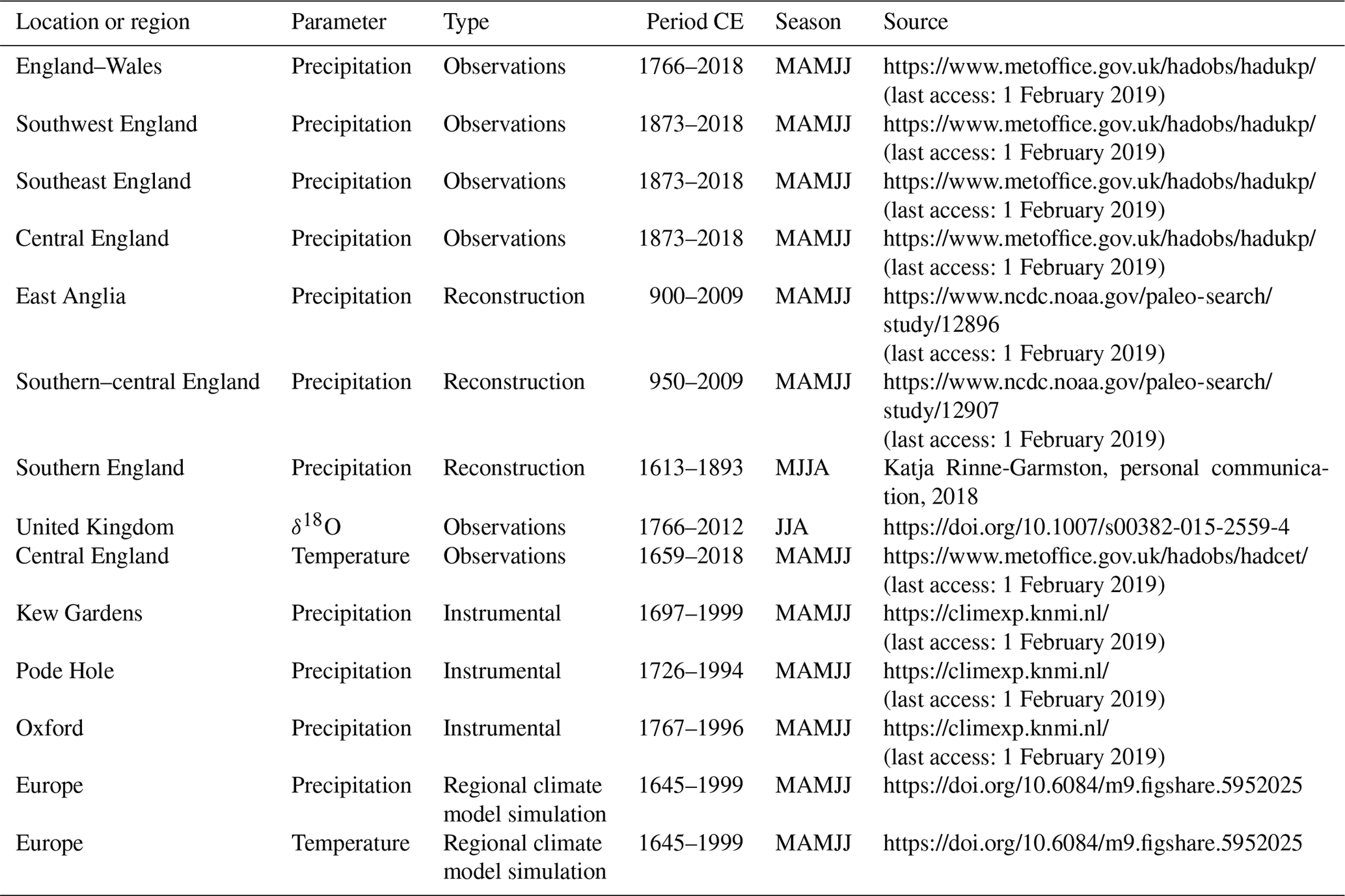
We use observationally derived data sets, reconstructions, and simulation output in our main analyses. We use further observationally derived records and instrumental station observations for assessing the quality of our main data sets. Table 1 lists the sources of information. For all analyses, we primarily use the spring–summer season from March to July (MAMJJ).

Starting from the available regional climate simulation (see below), we choose the region for our study based on the availability of precipitation observation and reconstruction data. There are long records of instrumental measurements of climate parameters for a number of locations in Europe. For southern Great Britain, there are observational regional domain composite records for temperature and precipitation, precipitation reconstructions, and long instrumental records.

2.1 Observations

The British Isles are unique because there are long observation-based indices for precipitation and temperature in the form of the England–Wales precipitation data (Alexander and Jones, 2000) and the Central England Temperature data (Parker et al., 1992). In addition, there are long instrumental station precipitation observations available, e.g., in southern Great Britain, for Kew Gardens, Oxford, and Pode Hole.

Alexander and Jones (2000, see also Wigley et al., 1984) describe the England–Wales precipitation (EWP) data. It is available from the Met Office Hadley Centre at monthly resolution extending back to the year 1766. The Met Office Hadley Centre also provides subdivisions of the data. We use those for southwest, southeast, and central England. Alexander and Jones (2000) describe the automated method of updating long precipitation series like the data by Wigley et al. (1984) while also ensuring the homogeneity of the data. Parker et al. (1992) similarly describe the production of the Central England Temperature data and how to maintain quality control and homogeneity.

The central England and England–Wales observation indices are good representations of the late 20th century climate of southern Great Britain according to Croxton et al. (2006). Note that the composite series naturally rely on the instrumental series.

The Climate Explorer (http://climexp.knmi.nl/, last access: 1 February 2019) provides access to a number of long series of monthly instrumental precipitation observations from the Global Historical Climatology Network (Peterson and Vose, 1997). We use those from Oxford, Kew Gardens, and Pode Hole in addition to the observationally derived Met Office Hadley Centre data sets. The Climate Explorer provides monthly data for these locations from 1697 to 1999, 1726 to 1994, and 1767 to 1999 CE, respectively. The later years in the Oxford record include missing values and we therefore only use data from 1767 to 1996 CE.

Frank et al. (2007) noted the uncertainties in early instrumental temperature observations. Additionally, the very early Central England Temperature data include noninstrumental indirect data to infer past temperature. Similarly, early precipitation observations require rigorous quality control (e.g., Burt and Howden, 2011). Woodley (1996) reviews the history of precipitation data for England and Wales as well as Scotland.

2.2 Reconstructions

There are a number of gridded reconstructions of hydroclimatic parameters covering the European domain. Continental domain gridded precipitation reconstructions include Pauling et al. (2006), Casty et al. (2007), and Franke et al. (2017). Reconstructions of drought indices like the PDSI exist as gridded products, too, for various regions of the world including Europe (The Old World Drought Atlas; Cook et al., 2015). These products allow for assessments of the quality of the hydroclimate in paleoclimate simulations (Smerdon et al., 2015).

We decide to use regional precipitation reconstructions for our domain instead of gridded products to minimize the effect of the reconstruction method on the results. We focus on precipitation as it allows for direct comparison with long instrumental records and it is a parameter directly experienced by people.

To our knowledge, there are three precipitation reconstructions for small domains from southern Great Britain, i.e., approximately within the domain of the England–Wales precipitation and the Central England Temperature data. These are for East Anglia (Cooper et al., 2013), for southern–central England (Wilson et al., 2013), and the reconstruction for southern England by Rinne et al. (2013). The former two use tree-ring-width data for their reconstructions, and the latter uses tree-ring oxygen isotopes. There is additionally the work by Young et al. (2015), who scale a δ¹⁸O composite record from Great Britain to the England–Wales precipitation.

In the main paper, we only use the data by Cooper et al. (2013) and Wilson et al. (2013) for, respectively, East Anglia and southern–central England in March, April, May, June, and July (MAMJJ). Cooper et al. (2013) and Wilson et al. (2013) identified this extended spring as the season to which their tree-ring-width records are sensitive for their reconstructions of precipitation. These authors calibrate their tree-ring data against gridded precipitation beyond their target regions of southern–central England and East Anglia, respectively. Thereby the reconstructions are possibly biased beyond their respective regions of interest. They compare their reconstructions against the long instrumental records and find a lack of stability in relation to the instrumental data. They discuss the limitations of their reconstructions, which represent less than 40 % of the regional precipitation variance over the 20th century. Obviously, the reconstructions suffer from the limited lengths of the available tree-ring samples. This may limit the resolution of precipitation variability at low frequencies in the reconstructions.

Although the reconstructions show a notable amount of low-frequency variability, Cooper et al. (2013) caution against too much confidence in the reconstructed low-frequency precipitation variability. Cooper et al. (2013) explicitly call their work “preliminary” with respect to reconstructing low-frequency precipitation variability. Wilson et al. (2013) and Cooper et al. (2013) emphasize the weaknesses of their reconstructions in representing extreme years. On the other hand, both are confident in the middle to high frequencies of their reconstructions.

The authors note variable relationships between tree growth and environmental controls for their regions in the past. Indeed, there are periods when the relationships between trees and precipitation are not significant. Wilson et al. (2013) and Cooper et al. (2013) discuss the possibility that the tree species used for their reconstructions were less sensitive to precipitation over certain periods, e.g., the early 19th century. That is, the proxies, theoretically representing a precipitation signal, also contain a temperature signal, for instance, if they are sensitive to soil moisture. Wilson et al. (2013) further suggest an effect of the Industrial Revolution and the associated pollution on the trees in their selection. Wilson et al. (2013) also discuss the reliability of the instrumental data but conclude this is likely not an issue.

The works by Rinne et al. (2013) and Young et al. (2015) use their δ¹⁸O data to reconstruct precipitation for southern England and Great Britain, respectively. We shortly discuss results for both reconstructions below and give some more details in the document in the Supplement.

Rinne et al. (2013) calibrate and scale their local isotope data from 1613 to 1893 CE against the station observations from Oxford for the period 1815 to 1893 CE and concatenate the reconstruction with the observations for 1894 to 2003 CE. They target an extended summer season from May to August.

Young et al. (2015) use the England–Wales summer (June to August) precipitation as a scaling target for a composite of eight isotope records from Scotland, Wales, and England for the period 1766 to 2012 CE. They provide the input series as a supplement to their paper.

Both publications by Rinne et al. (2013) and Young et al. (2015) note the differences of their scaled δ¹⁸O data to the tree-ring-width-based works by Wilson et al. (2013) and Cooper et al. (2013). Young et al. (2015) emphasize that the extended spring reconstructions are basically unrelated to the δ¹⁸O data. Young et al. (2015) conclude that these differences make it unlikely that the tree-ring-based works and their δ¹⁸O-based work represent the same environmental parameter. They highlight the lack of a calibration against regional precipitation data. Young et al. (2015) conclude that their own data reliably reflect precipitation, while the tree-ring widths most likely represent the combination of various environmental influences on tree growth instead of a single climate parameter.

Despite the conclusions of Young et al. (2015) we decide to focus in the main paper on the two tree-ring-width-based records by Cooper et al. (2013) and Wilson et al. (2013). The main reason for excluding the Rinne et al. record is that it concatenates instrumental data from the Radcliffe (cf. Oxford) station for 1894 to 2003 to the reconstructed values from 1613 until 1893. This reduces the time of overlap with the England–Wales precipitation data.

We do not focus on the data by Young et al. (2015) for two reasons. Firstly, the authors do not provide the full reconstruction, and, secondly, the data start at the earliest in 1766 CE, which again minimizes the period available for comparing to the simulation data.

We think the focus on the tree-ring-width-based reconstructions is appropriate to present the possibilities of using the SPI and to highlight potential consistencies and inconsistencies between the different data sources. In the following, we compare the two reconstructions for southern Great Britain with the England–Wales precipitation observations.

2.3 Simulations

We compare the observations and the reconstructions to output from a regional simulation with the model CCLM for the European domain over the period 1645 to 1999 as also used by Gómez-Navarro et al. (2014) and Bierstedt et al. (2016). We use output from 1652 onwards (Gómez-Navarro et al., 2014). To our knowledge, this simulation is one of only two transient regional simulations for this region and the last few centuries.

Forcing for the regional simulation is from a global simulation with the Max Planck Institute Earth System Model (MPI-ESM) in its Millennium simulation COSMOS setup. For details, see Jungclaus et al. (2010). This version of MPI-ESM couples the atmosphere model ECHAM5, the ocean model MPI-OM, a land-surface module including vegetation (JSBACH), a module for ocean biogeochemistry (HAMOCC), and an interactive carbon cycle. For the simulation, ECHAM5 was run with a T31 horizontal resolution and with 19 vertical levels. MPI-OM used a variable resolution between 22 and 250 km on a conformal grid for this simulation. The ensemble used diverse forcings. The driving simulation for the regional simulation with CCLM is one MPI-ESM simulation with all external forcings and a reconstruction of solar activity based on Bard et al. (2000), i.e., with a comparatively large amplitude of solar variability.

The regional climate model CCLM simulation (Sebastian Wagner, personal communication, 2014, 2015, 2018; see also Gómez-Navarro et al., 2014; Bierstedt et al., 2016) uses adjusted forcing fields relevant for paleoclimate simulations as also used with the global MPI-ESM simulation. These include orbital forcing and solar and volcanic activity. Since the regional model does not represent the stratosphere, the regional simulation considers the effect of volcanic aerosols as a reduction in solar constant equivalent to the net solar shortwave radiation at the top of the troposphere in MPI-ESM. CO₂ variability is prescribed and changes in the greenhouse gases CO₂, CH₄, and N₂O are based on data by Flückiger et al. (2002). Land-cover changes are included as external lower boundary forcing using the same data set as the MPI-ESM simulation (Pongratz et al., 2008). The presented CCLM simulation uses a rotated grid with a horizontal resolution of 0.44 by 0.44^∘ and 32 vertical levels. The sponge zone of seven grid points at each domain border is removed and fields are interpolated onto a regular horizontal grid of 0.5 by 0.5^∘.

We choose the domain including grid points closest to the longitudinal and latitudinal borders 5.5^∘ W to 1.5^∘ E and 50.5 to 54.5^∘ N to represent the England and Wales precipitation domain. This selection is somewhat arbitrary but we assume it sufficiently represents the England–Wales precipitation domain to allow for a meaningful comparison of changes in percentiles, although not in absolute percentile values. We choose the domain 5 to 0^∘ W and 50 to 55^∘ N as the simulated counterpart of the Central England Temperature data. The simulated East Anglia series represents the domain 0 to 2^∘ E and 52 to 53^∘ N, and we choose the domain 2.5^∘ W to 0^∘ E and 51 to 52.5^∘ N as equivalent for southern–central England. All analyses are for the extended spring season, MAMJJ, since this is the seasonal focus of the reconstructions. The Appendix provides a short evaluation of the simulation against the observational CRU data (Harris et al., 2014) over the European domain. We do not apply any bias correction to the simulation output.

So far, global simulations for the last millennium have notably coarser resolutions than the 0.44 by 0.44^∘ of the regional simulation we use here (compare, e.g., Fernández-Donado et al., 2013; PAGES 2k-PMIP3 Group, 2015). However, in contrast to present-day and future scenario regional simulations, a 0.44 by 0.44^∘ resolution represents a comparatively coarse-resolution dynamical downscaling. As a review by Ludwig et al. (2018, including two of the present authors) highlights, this is because the demand for long simulation periods limits applications of regional models in paleoclimatology to relatively coarse setups. Thus, one may question the benefits of the approach compared to more recent higher-resolution global simulations, e.g., with the global models CCSM4 and CESM1 (Landrum et al., 2012; Lehner et al., 2015), which have resolutions of $\mathrm{0.9}{}^{\circ }\times \mathrm{1.25}{}^{\circ }$.

Sørland et al. (2018) discuss the benefits of regional climate simulations in studies on regional climates. Besides other models, they also use CCLM in a 50 km setup comparable to the simulation used here. They note that improved representation of regional climate in a regional simulation is not solely due to the increased resolution but may also be due to different strategies in model building and tuning. Pinto et al. (2018) explain differences in results from regional, including CCLM, and global simulations for southern Africa with an interplay between the representation of sub-grid-scale processes in the different models and factors related to the increased resolution.

Blenkinsop and Fowler (2007) find that regional climate models may be deficient in their ability to model persistent low precipitation episodes for the British Isles, which has repercussions for their representation of drought events. The review by Ludwig et al. (2018) reports more realistic distributions for precipitation in regional paleoclimate simulations.

Flato et al. (2013, chapter 9 of the IPCC AR5) review the progress of regional downscaling and high-resolution modeling. They emphasize that the skill of such exercises depends on the model used, the season, the domain of interest, and the considered meteorological variable. They highlight studies showing that there is not a linear increase in simulation skill towards higher resolutions. Higher resolutions typically provide more reliable estimates of extremes, including heavy rainfall.

The quality of the simulated precipitation still strongly depends on the parameterizations implemented in the regional climate model. Precipitation, especially convective precipitation events, is still a sub-grid process, even within regional climate models. Concentrating on accumulated amounts on seasonal timescales and their long-term changes, however, allows for a more robust comparison of simulated precipitation to observed and reconstructed data.

3 Methods

One objective of this paper is to highlight how the concept of the Standardized Precipitation Index (SPI; McKee et al., 1993) adds additional perspectives when comparing various sources of information for periods with and without instrumental observations. Therefore, we shortly introduce the SPI transformation procedure and how we use this information to subsequently compare precipitation estimates from observations, reconstructions, and a regional climate simulation.

3.1 The Standardized Precipitation Index – SPI

Standardizing precipitation data facilitates comparing precipitation distributions between different locations, timescales, periods, and data sources. For this purpose, McKee et al. (1993) introduced the Standardized Precipitation Index (SPI).

The Interregional Workshop on Indices and Early Warning Systems for Drought proposed the SPI as a common index to facilitate comparability between meteorological drought estimates for different regions (see also Keyantash et al., 2002; Hayes et al., 2011). The SPI should complement previously used indices.

Raible et al. (2017) find the SPI to be a reliable drought index for western Europe including the British Isles. The standardization inherent to the SPI allows for further applications, e.g., flood monitoring (Seiler et al., 2002), and the easy comparison of normal, dry, and wet conditions between different sources of data. Indeed, the UK drought portal (https://eip.ceh.ac.uk/droughts, last access: 1 February 2019) relies on the SPI. Sienz et al. (2012) discuss associated biases of the approach.

The SPI uses only precipitation, which makes it an ideal and relatively straightforward tool for comparing hydroclimatic data between different data sources. Precipitation is a standard output of simulations and there are long instrumental records for various locations and a number of reconstructions as well.

However, as the SPI uses only precipitation, it is of less value when the interest is in, e.g., the water supply, runoff, or streamflow (but see Seiler et al., 2002). The focus on precipitation also limits the applicability for studying temperature-sensitive parts of the hydrological cycle and impacts on biological and anthropogenic systems (e.g., PAGES Hydro2k Consortium, 2017; Keyantash et al., 2002; Hayes et al., 2011; Van Loon, 2015).

Previous usage of the SPI in paleoclimatology focused on the index series. For example, Domínguez-Castro et al. (2008) and Machado et al. (2011) compare SPI series to differently derived hydroclimatic indices over approximately the last 500 years. Other studies reconstructed the SPI instead of absolute precipitation amounts (e.g., Seftigen et al., 2013; Yadav et al., 2015; Tejedor et al., 2016; Klippel et al., 2018). Lehner et al. (2012) use the SPI to compute pseudo-proxies from reanalysis data and long simulations with global climate models to test a reconstruction method.

3.1.1 Transformation

The SPI requires fitting a distribution function to the precipitation data and there are various candidate distributions (e.g., Sienz et al., 2012; Stagge et al., 2015, and their references). In our analyses, we fit a Weibull distribution. Sienz et al. (2012) highlighted the fact that the Weibull distribution performed better in transforming the England–Wales precipitation data on a monthly timescale compared to a number of other distributions. However, other distributions outperformed the Weibull distribution for other data sets and other SPI timescales. Results differ only little if we fit gamma or generalized gamma distributions (not shown). Our procedure of the SPI calculation follows the detailed description by Sienz et al. (2012).

McKee et al. (1993) recommend at least 30 data points for successful distribution fits, but Guttman (1994) notes the lack of stability for small sample sizes. We fit distributions over sliding 51-year windows. Thus, we use more data points than recommended by McKee et al. (1993) but still fewer than the 60 points for which Guttman (1994) finds convergence of higher-order L moments. Appendix Fig. B1 shows 95 % intervals of a bootstrap procedure sampling 40 data points 1000 times from each window and fitting distributions to these samples. The choice of 40 data points is an ad hoc decision. We could have also chosen sample sizes of 49 data points.

3.1.2 Evaluation

Standardizing precipitation data can at least attenuate some of the problems mentioned in the Introduction. Transforming precipitation to standardized values provides further means to study the agreement or the lack thereof between different data sources.

By transforming to the SPI over moving windows, we essentially compare climatologies and potentially filter shorter-term internal variability. If the climatology for the observations is the target climatology, an ensemble of climate simulations should sample this distribution following the paradigm of a statistically indistinguishable ensemble (Annan and Hargreaves, 2011). Our analyses compare how well the climatologies agree in different sources of data.

One particular interest is to consider to what extent the different data sources describe comparable evolutions in various percentiles, e.g., representing extremes. The SPI transformation simplifies this. If the transformation over moving windows filters a certain amount of internal variability, if boundary and forcing conditions are sufficiently equivalent in the simulation compared to the observed climate, and if simulated precipitation and the observed climate react equivalently to these conditions, precipitation distributions and their properties may change consistently between different sources of information. The results of Gómez-Navarro et al. (2015) give some indications that this expectation may be warranted. In the worst case, our analyses can point out that one of the data sources contradicts the others.

For any given window, the fitted distribution parameters allow for the calculation of various properties. For example, we can consider the changing amount of precipitation, which one would describe as average, extremely high, or extremely low for subsequent periods. In the SPI literature, percentiles 6.7 and 93.3 traditionally represent the regions of severe (and extreme) dryness and wetness of the probability density function. Accordingly, we subsequently compare percentiles 6.7 and 93.3 for the fitted distributions over time. Further, we can compare the moments of the distributions. We choose to show the square root of the Weibull distribution variance, i.e., the Weibull standard deviation over sliding windows. This provides an additional clarification of how the precipitation distribution changes over time. Appendix C shows parameters for the distribution fits.

The fitted parameters allow for further analyses; e.g., we can compare how likely a reference amount of precipitation is for different periods. We do this for percentiles 50, 6.7, and 93.3 in a reference year. We choose 1815 CE as the reference year, since it is included in all data sets and it allows for potentially equivalent analyses of the PMIP3 past1000 simulations (e.g., Schmidt et al., 2011).

3.2 Smoothing

Performing the transformation to standardized precipitation over 51-year windows results in smoothed estimates. For convenience, we additionally plot smoothed time series in a number of figures. Filtered series are solely used for visualization.

We use a Hamming window. In most cases, this has a length of 51 points but we also occasionally use different window lengths. The 51-point Hamming filter represents a different frequency cutoff than a simple 51-year moving median or moving mean as can be obtained from fitting the distributions over 51-year moving windows.

4 Results

4.1 Relations among data sets

4.1.1 Observational data and reconstructions

Figure 1 provides a first impression of the observational and reconstruction data we use in the following sections. All series are for the extended spring season from March to July on which we focus. Panels show 31-point Hamming-filtered time series. These allow for a better qualitative assessment of the commonalities between the data sets and the differences compared to, e.g., 11-point or 51-point Hamming-filtered time series, which have too much high-frequency variability or are too smoothed, respectively.

Observational precipitation series from the Met Office Hadley Centre for southwest, southeast, central England, and England–Wales show high agreement in their variations on these timescales for the period of overlap (see Fig. 1a, particularly the period 1890 to approximately 1980). The instrumental time series for Kew Gardens and Pode Hole show more disagreement in certain periods for the considered smoothing; i.e., they even evolve oppositely at certain times, e.g., the mid-19th and mid-20th centuries (see Fig. 1b). The instrumental data for Oxford appear to agree better with the data for Kew Gardens, which is to be expected from the geographic locations of the stations. Visually, both reconstructions agree less well with the observational series and with each other than the agreement amongst the observational data (see Fig. 1c). This holds for their variations and their overall level of variability. Figure 1d adds the Central England Temperature data for MAMJJ for completeness.

Figure 1 Visualization of the observation-based records for the extended spring season March to July (MAMJJ). We show 31-point Hamming-filtered time series for (a) the Met Office Hadley Centre observational precipitation series for England–Wales (EWP), southwest (SWE), southeast (SEE), and central England (CEP), (b) the instrumental precipitation series for Pode Hole (Pod), Kew Gardens (Kew), and Oxford (Oxf), (c) the precipitation reconstructions for East Anglia (EAr) and southern–central England (SCEr), and (d) the Central England Temperature (CET) data.

Correlation matrices (Fig. 2 and the Supplement) and scatterplots (see the Supplement) emphasize the differing agreement between the various data sources even more clearly. Figure 2 presents the correlation matrix for complete observations, i.e., for the period 1873 to 1994 when all records have data. Correlation coefficients change slightly if we consider pairwise complete records. Relations among precipitation data sets are always positive. They are very strong between the England–Wales data and its subdivisions, between the Kew Gardens series and the southeast England data, between the Pode Hole series and the central England data, and between the Oxford record and the southeast England data as well as the England–Wales precipitation. The relationship between the two reconstructions is also rather strong over the subperiod. Correlations are, however, weaker between the reconstructions and the observed series.

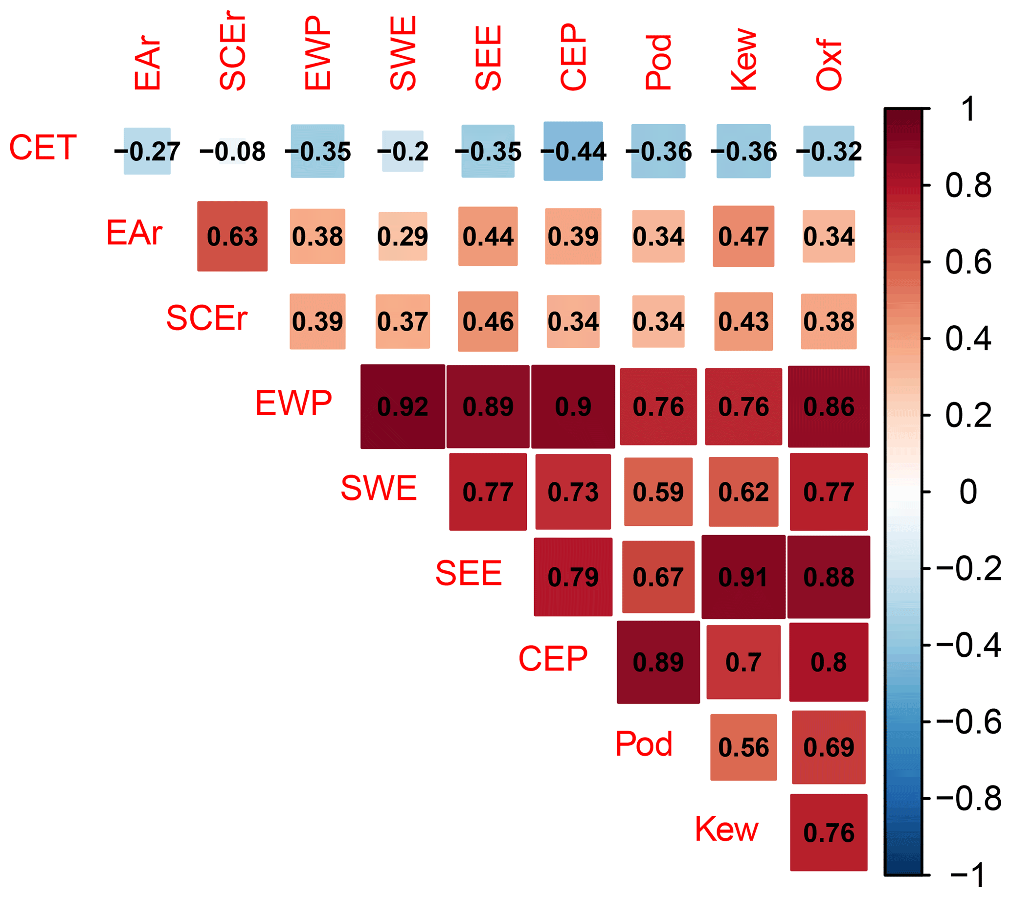
Figure 2 Correlation matrix for complete correlations between the observation- or paleo-observation-based data sets Central England Temperature (CET), East Anglia precipitation reconstruction (EAr), southern–central England precipitation reconstruction (SCEr), England–Wales precipitation (EWP), southwest England precipitation (SWE), southeast England precipitation (SEE), central England precipitation (CEP), Pode Hole precipitation (Pod), Kew Gardens precipitation (Kew), and Oxford precipitation (Oxf). Complete correlations mean that we only use the years 1873 to 1994 for which all records have data. The season for all records is MAMJJ.

There is a generally negative relationship between the Central England Temperature and the precipitation data sets for the chosen extended spring season from March to July. It is weakest for the southern–central England reconstruction but also rather weak for the East Anglia reconstruction and the southwest England record from the Met Office Hadley Centre. Scatterplots emphasize that even the temperature–precipitation relations with larger correlations scatter widely (not shown). Temperature relations are stronger for the observationally based data from the Met Office Hadley Centre and the instrumental series for the summer season June to August (not shown).

Correlations for nonoverlapping 11-year averages are positive and strongest between the England–Wales precipitation and the two instrumental series (not shown; see the Supplement; calculated for the period 1767 to 1986). This analysis also gives reasonable correlations (r≈0.51) between the pair of reconstructions and between the instrumental series. Otherwise, correlations are weak. Correlations for the extended spring season with the Central England Temperature data are largest for the nonoverlapping 11-year averages of the Kew Gardens instrumental series. We choose 11-year nonoverlapping windows to balance the number of available data points and the filtering of interannual variability.

4.1.2 (Paleo-)observational data and regional simulation output

Figure 3 presents the two reconstructions and the England–Wales precipitation in comparison to the respective data from the regional simulation. All data are again for the extended spring season from March to July (MAMJJ), and the panels zoom in on the period of the regional simulation. We show the interannual time series and the 51-point Hamming-filtered representation.

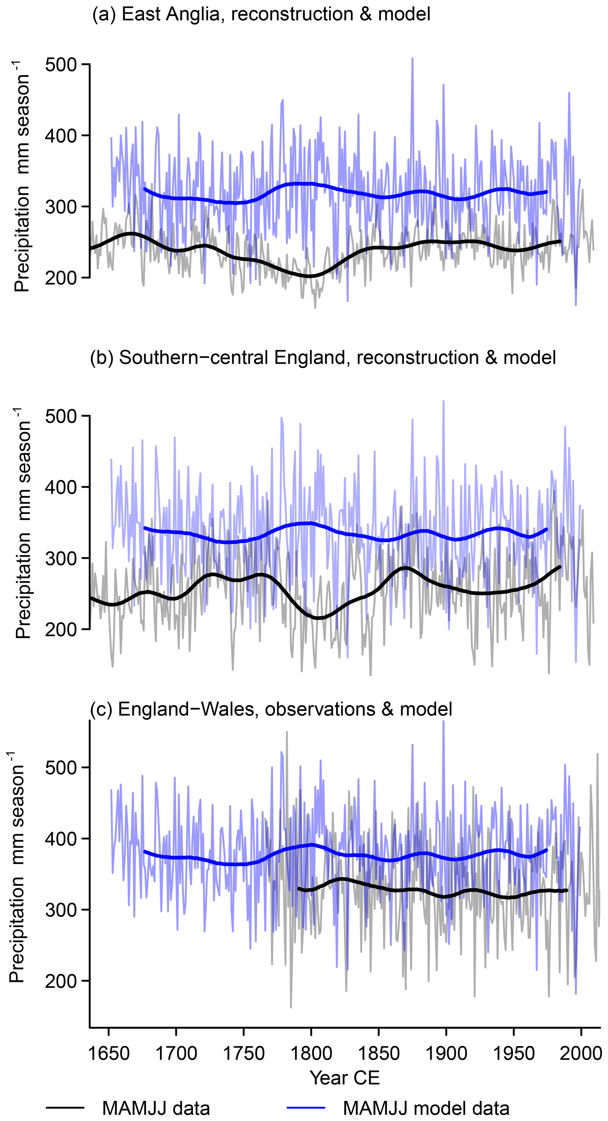
Figure 3 Extended spring (MAMJJ) precipitation in (paleo-)observation-based data and simulation output, (a) East Anglia precipitation in reconstruction (black) and regional model (blue), (b) southern–central England precipitation in reconstructions (black) and regional simulation (blue), and (c) England–Wales precipitation in observational data (black) and regional simulation (blue). We show interannual data (light colors) and 51-point Hamming-filtered data (solid colored).

Considering the evolution of the records, the 51-point Hamming-filtered time series show pronounced differences besides some common features for the reconstructions for southern–central England (Wilson et al., 2013) and East Anglia (Cooper et al., 2013) (black lines in Fig. 3a and b) similar to the representations in Fig. 1. Both reconstructions feature a relative precipitation minimum centered on approximately the year 1800. The southern–central England reconstruction additionally displays a relative minimum in the early 20th century.

The observed England–Wales precipitation is available at monthly resolution from the year 1766 onward. The Hamming-filtered time series shows markedly less multi-decadal to centennial variability compared to the reconstructions, but the observations have much more interannual variability than the reconstruction for East Anglia and slightly more variability than the reconstruction for southern–central England (Fig. 3c, black line). The filtered England–Wales time series also displays a slightly negative trend.

Differences between the simulated regional records are generally smaller (blue lines in Fig. 3). Existing differences highlight the spatial heterogeneity of precipitation, e.g., interannual pairwise correlation coefficients are about 0.9 between the simulated East Anglia data and the other two records, while the simulated England–Wales precipitation correlates at approximately 0.97 with the simulated southern–central England data. Absolute interannual precipitation differences among the three data sets are at a maximum of approximately 151 mm season⁻¹ (not shown). A general feature for all regions is that the excursions of the filtered simulation output are often, but not always, opposite to those of the reconstructions or observation time series.

There is an obvious bias in the absolute amounts between the simulation output and the other data sets. The simulation output series give larger precipitation amounts. We do not try to attribute this difference. We note that it is not as prominent for the more local comparison with the data from Rinne et al. (2013) for May to August and the bias is generally slightly negative for the summer season June to August for England–Wales precipitation (not shown; see the Supplement). We assume that the differing spatial representations sufficiently explain the mismatch. However, the change of sign in the bias for the summer season suggests that the simulation overestimates spring precipitation, underestimates summer precipitation, and the positive spring bias is larger than the negative summer bias. See also Appendix A for a comparison of the simulation to observational data over the full European model domain. Figure 3 shows a common feature for all three comparisons. Simulated records appear to show opposite evolutions compared to the (paleo-)observations overall but particularly in the late 18th to early 19th century and in the early to mid-20th century.

This initial comparison already shows varying levels of agreement for the chosen data sets derived from observations and the reconstructions. It highlights the fact that the relationships between the reconstructions and the observational data sets are weaker than between the instrumental data and the observational indices on interannual timescales. Note that the regional observational indices include information from the instrumental data. On longer timescales the reconstructions align less well among each other than the observationally derived time series. However, the local, purely instrumental series also show more disagreement among each other than the derived larger-domain products. Filtered regional time series often evolve visually oppositely in the simulation compared to the reconstructions and the observations.

So far, we used the precipitation and temperature data. In the following, we mainly use the information obtained via the transformation to standardized precipitation indices.

4.2 Comparing standardized precipitation data

Figures 4 to 6 add, respectively, the comparisons of the wet (i.e., 93.3) percentile, the dry (i.e., 6.7) percentile, and the square root of the Weibull distribution variance to the comparison of the interannual and filtered time series in the previous section.

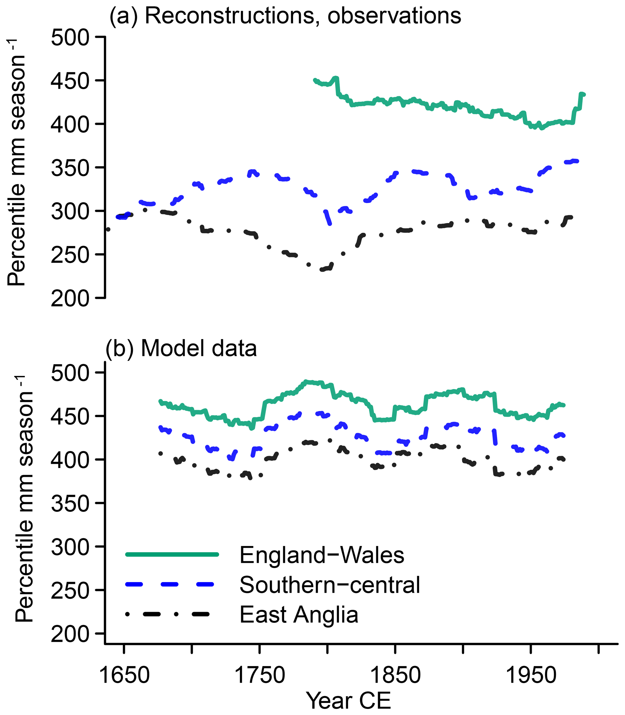
Figure 4 Visualization of the MAMJJ precipitation amount identified as severely wet (percentile 93.3) over 51-year windows for England–Wales (green solid lines), southern–central England (blue dashed lines), and East Anglia (black dash-dotted lines) in (a) reconstructions, observations, and (b) simulations.

4.2.1 Observations vs. reconstructions

Since they represent different regions, we do not expect agreement in the absolute precipitation amounts representing wet conditions between the England–Wales precipitation data and the reconstructions in Fig. 4a. We note that the difference between the wet percentile for the England–Wales precipitation and the reconstructions is larger than for the average amounts, indicating a wider distribution for the data based on instrumental observations. Precipitation histograms confirm this (not shown). On the other hand, differences are smaller for the dry percentile (Fig. 5). Nevertheless, this is a sign that the reconstructions underestimate the width of the precipitation distributions of 51-year window climatologies.

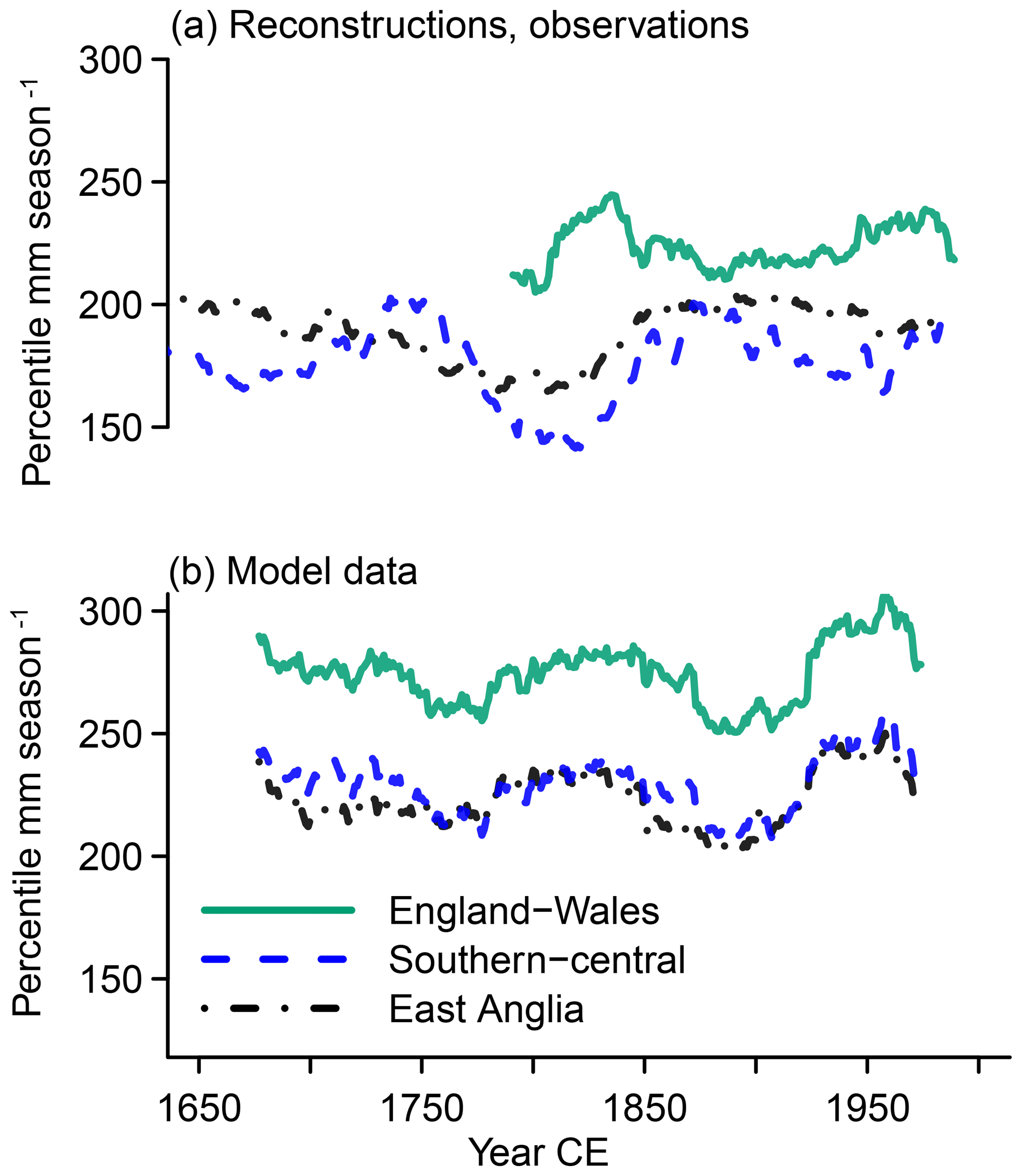
Figure 5 Visualization of the MAMJJ precipitation amount identified as severely dry (percentile 6.7) over 51-year windows for England–Wales (green solid lines), southern–central England (blue dashed lines), and East Anglia (black dash-dotted lines) in (a) reconstructions, observations, and (b) simulations.

Reconstructed and observation-based time series show a slightly opposite trend for the wet percentile over much of the period of their overlap (Fig. 4) from the second half of the 18th century to the mid-20th century. Smaller-amplitude variations in the beginning of the wet percentile series are also opposite. The dry percentile series do not have a long-term trend but multi-decadal variations evolve oppositely between reconstructed and observed dry percentiles from the end of the 18th century to the early 20th century (Fig. 5).

The opposite trends in the wet percentiles mean that the wet percentile represents lower precipitation amounts in the middle of the 20th century compared to the late 18th century, while the reconstructed wet percentile represents larger precipitation amounts in the middle of the 20th century compared to the late 18th century (Fig. 4). Similarly, the opposite multi-decadal variability in the dry percentiles of reconstructions and observations means that when the reconstructions represent a drying of the dry percentiles, the observations indicate the opposite and vice versa (Fig. 5). Generally, the series for the severe to extreme dryness and wetness percentiles reflect the smoothed evolution of the respective data set before transformation into a distributional form (compare Fig. 3).

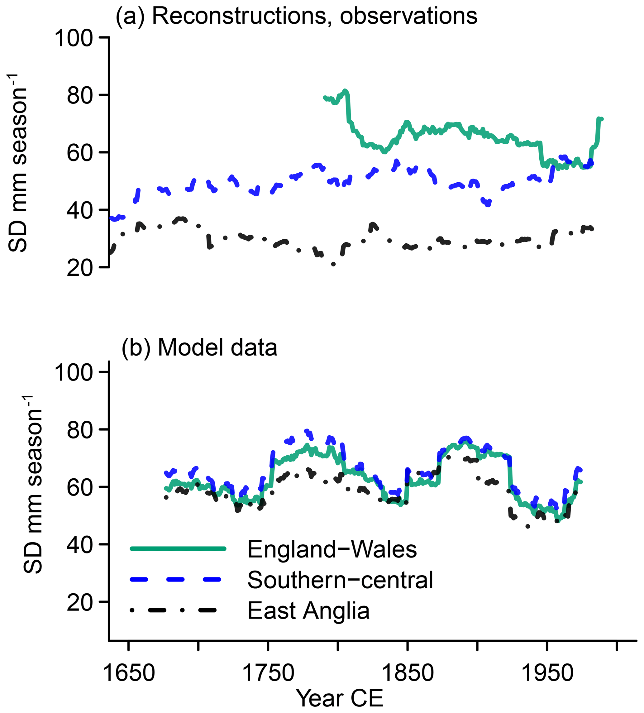
Figure 6 Visualization of Weibull standard deviations (SDs) over 51-year windows for MAMJJ precipitation for England–Wales (green solid lines), southern–central England (blue dashed lines), and East Anglia (black dash-dotted lines) in (a) reconstructions, observations, and (b) simulations.

We note that the data from Rinne et al. (2013) for southern England in summer display an apparent opposite evolution of wet percentiles for the period of overlap between reconstructions and observations from the late 18th to the late 19th century. On the other hand, dry percentiles agree well over this period (not shown; see the Supplement).

Parameters for the fitted distributions also allow us to evaluate the moments of the distributions. Estimates for the Weibull standard deviations (SDs in Fig. 6) differ between observations and reconstructions as expected from the previously noted differences in percentiles. The reconstruction for East Anglia does not show a clear evolution in the Weibull standard deviations, whereas there is an increasing trend in the Weibull standard deviations for the southern–central England data. The observations show a slight reduction in the standard deviation until the middle of the 20th century, with a strong increase afterwards.

4.2.2 Simulation output

The simulated time series in Fig. 3 show large similarities between regions. This is also the case for the wet and dry percentiles as well as for the standard deviations. Indeed, the respective statistics evolve simultaneously among the different regions, and the standard deviations overlap (Figs. 4 to 6).

Thus, differences between regional domains are smaller for their simulated representations compared to the observed or reconstructed records. They are slightly more notable for the moving window statistics compared to the Hamming-filtered series. Dry percentiles are very similar for East Anglia and southern–central England in the simulation but wet conditions require larger precipitation amounts for southern–central compared to East Anglia. Appendix B highlights the fact that this may be due to sampling variability. Smoothed simulated data and wetness percentiles evolve similarly, but opposite evolutions of the dryness and wetness percentiles result in widening and shrinking of the distributions after approximately the year 1800.

4.2.3 Simulation output vs. observationally derived data and reconstructions

Simulations and reconstructions do not agree on the time evolution of precipitation percentiles (Figs. 4 to 6). Any hint of an agreement between reconstructed and simulated data is likely due to randomness (compare Fig. 4). There is instead a tendency towards opposite time evolutions between the data sources. This is best seen in the dry percentiles from the mid-18th to mid-20th century (Fig. 5).

This apparent opposite evolution is the most common feature when comparing percentiles derived from the simulation and from the reconstructions. When the percentile series for the reconstructions show minima, the simulation commonly shows maxima and vice versa. Obviously, using an ensemble of regional simulations would show a range of trajectories. Therefore, these results do not preclude the possibility that the model is capturing basic physical characteristics of precipitation variability in northwestern Europe.

The smoothed representations of the simulation output and the smoothed observed England–Wales precipitation show only small multi-decadal variations, which appear to be more or less in opposition (Fig. 3). The wet percentiles do not show any agreement although they both have a relative maximum in the late 18th century (Fig. 4). On the other hand, the dry percentiles show approximate agreement in their evolutions over the full time period of their overlap. Particularly noteworthy are the approximately concurrent maxima in the early 19th century and in the middle of the 20th century (Fig. 5). Similarly, the Weibull standard deviations show some commonalities between the simulated representation of the England–Wales precipitation and the observations (Fig. 6) over the full period of their overlap.

We note that there is neither any clear commonality nor any overly opposite evolution in the dry percentiles when comparing the regional simulation to the reconstruction for southern England summer precipitation by Rinne et al. (2013, not shown; see the Supplement). The wet percentiles, however, evolve oppositely in the 18th century but then show a common positive trend in the 19th century (not shown; see the Supplement).

Figure B1 provides uncertainty estimates for part of our analyses. The figure shows 95 % intervals of a bootstrap procedure sampling 40 data points 1000 times from the time windows and fitting distributions to these samples. The choice of 40 data points is an ad hoc decision that lies between the recommendation by McKee et al. (1993) of 30 samples and our window length of 51 years. Uncertainty on the fitted distributions varies in size over time and between data sets. Indeed, there are periods when sampling variability is so large that apparent differences in distributional properties between periods are not significant for most sources of information.

4.3 Changes in probability of certain precipitation amounts

In the Methods section, we describe the procedure for calculating standardized precipitation indices over moving time windows. We obtain a distribution fit for each time window. The parameters of the fit for a window allow us to identify the probability of a precipitation amount for the respective window. Figures 7 to 9 present changes in the probability of certain amounts of precipitation; i.e., lines are the changing percentiles represented by a given amount of precipitation over time. The figures show these changes for the precipitation amounts representing percentiles 93.3, 50, and 6.7, respectively, in a reference window. For this comparison, the reference is the distribution of precipitation in the window centered around the year 1815 CE. The year 1815 CE is included in all data sets and it allows for equivalent analyses of the PMIP3 past1000 simulations (e.g., Schmidt et al., 2011). We estimate and plot the percentiles that correspond to these reference precipitation amounts in other time windows.

Figure 7 Visualization of how percentile values change over windows. We show what the percentile 93.3 MAMJJ precipitation amount for a reference window represents over time for England–Wales (green solid lines), southern–central England (blue dashed lines), and East Anglia (black dash-dotted lines) in (a) reconstructions, observations, and (b) simulations. The reference window is centered on 1815 CE.

The England–Wales precipitation shows a slight increase over time in the reference percentile 93.3 in the year 1815 CE (Fig. 7a). Recently, there has been a steep decrease in the series. Similarly, the 50th percentile for 1815 CE represents slightly larger percentiles over time (Fig. 8a). On the other hand, there are weak multi-decadal variations in the series for percentile 6.7 in the observations, and percentile 6.7 from 1815 CE may become slightly less likely over time (Fig. 9a).

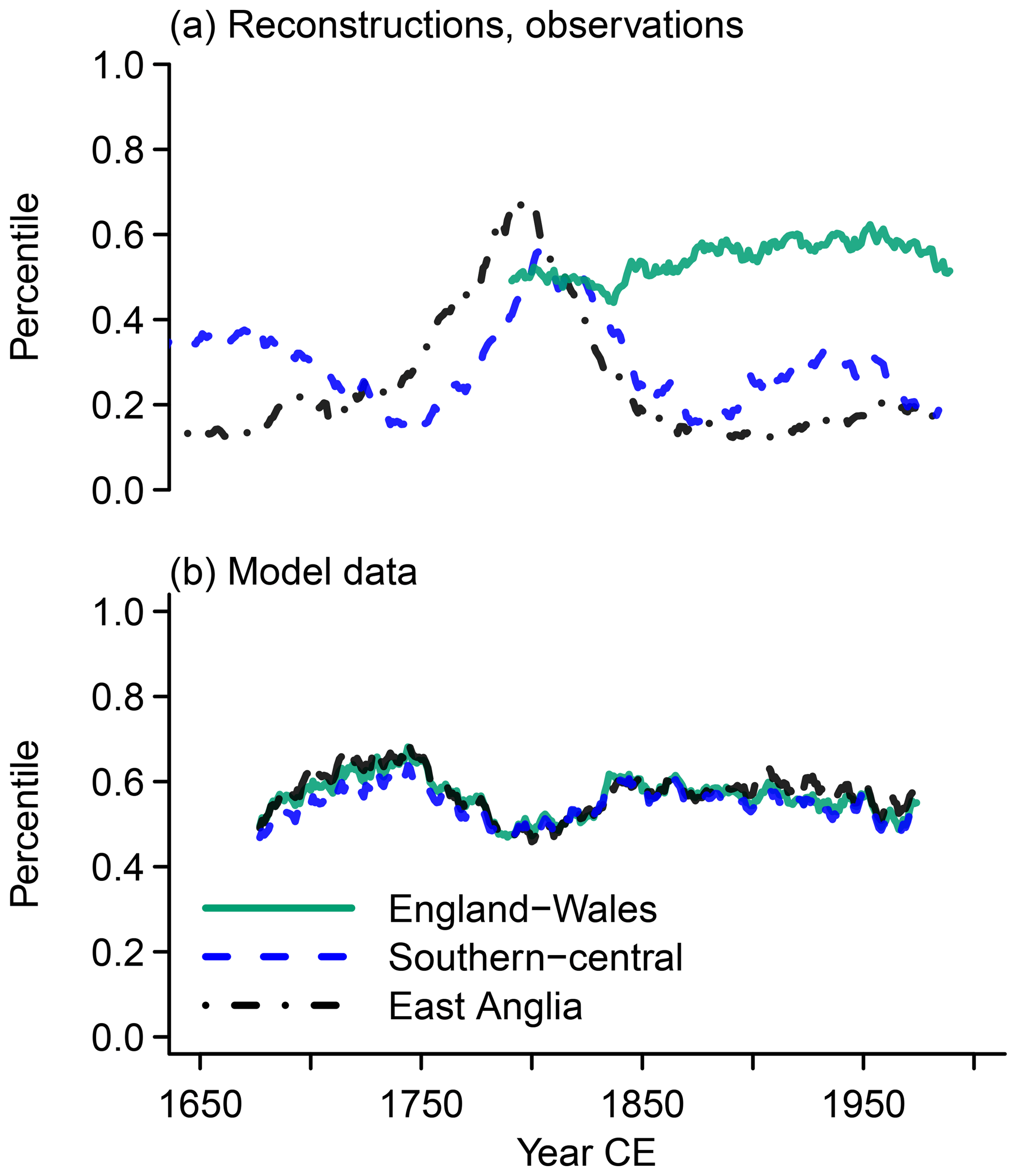
Figure 8 Visualization of how percentile values change over windows. We show what the 50th percentile MAMJJ precipitation amount for a reference window represents over time for England–Wales (green solid lines), southern–central England (blue dashed lines), and East Anglia (black dash-dotted lines) in (a) reconstructions, observations, and (b) simulations. The reference window is centered on 1815 CE.

Before turning to the reconstructions, we shortly note that the simulations show similar trajectories for all three percentile values and all three regions. There are not any obvious trends, but the series show multi-decadal variations. The window centered on the year 1815 CE falls within a minimum or at the end of a minimum. The respective precipitation amount generally represents larger percentiles before the time window centered on 1815 CE. After this time window, percentiles 6.7 and 93.3 both approach a maximum in the series (Figs. 7b and 9b). However, percentile 93.3 reaches it about the year 1850 CE and the percentile 6.7 only in approximately the year 1900 CE, when percentile 93.3 is again in a relative minimum. Thus, the wet and dry percentiles evolve oppositely from the early 19th century onwards; i.e., the distribution widens and shrinks since approximately the year 1850 CE. The amount of precipitation, which represents median values for the reference year 1815 CE, is representative of larger percentiles in later years (Fig. 8b). However, there is a slight decreasing trend from approximately the mid-19th century to the end of the simulation (Fig. 8b).

The reconstructions for East Anglia and southern–central England have some peculiar features (Figs. 7a to 9a). For one, it is not ideal to choose a reference year from the period around 1800 CE. Percentile 6.7 in 1815 CE is much less likely earlier and later in both regions (Fig. 9a). Similarly, average precipitation around 1815 CE represents approximately the 20th percentiles in earlier and later periods for East Anglia (Fig. 8a) but also represents much smaller percentiles in later periods for southern–central England. Severe and extreme wet conditions from this period may even represent long-term average conditions for East Anglia (Fig. 7a). We note that comparisons to the data by Rinne et al. (2013) do not feature such peculiarities (not shown), but using a simple scaling approach for the δ¹⁸O data from Young et al. (2015) gives similar results (not shown, but compare information given in the Supplement).

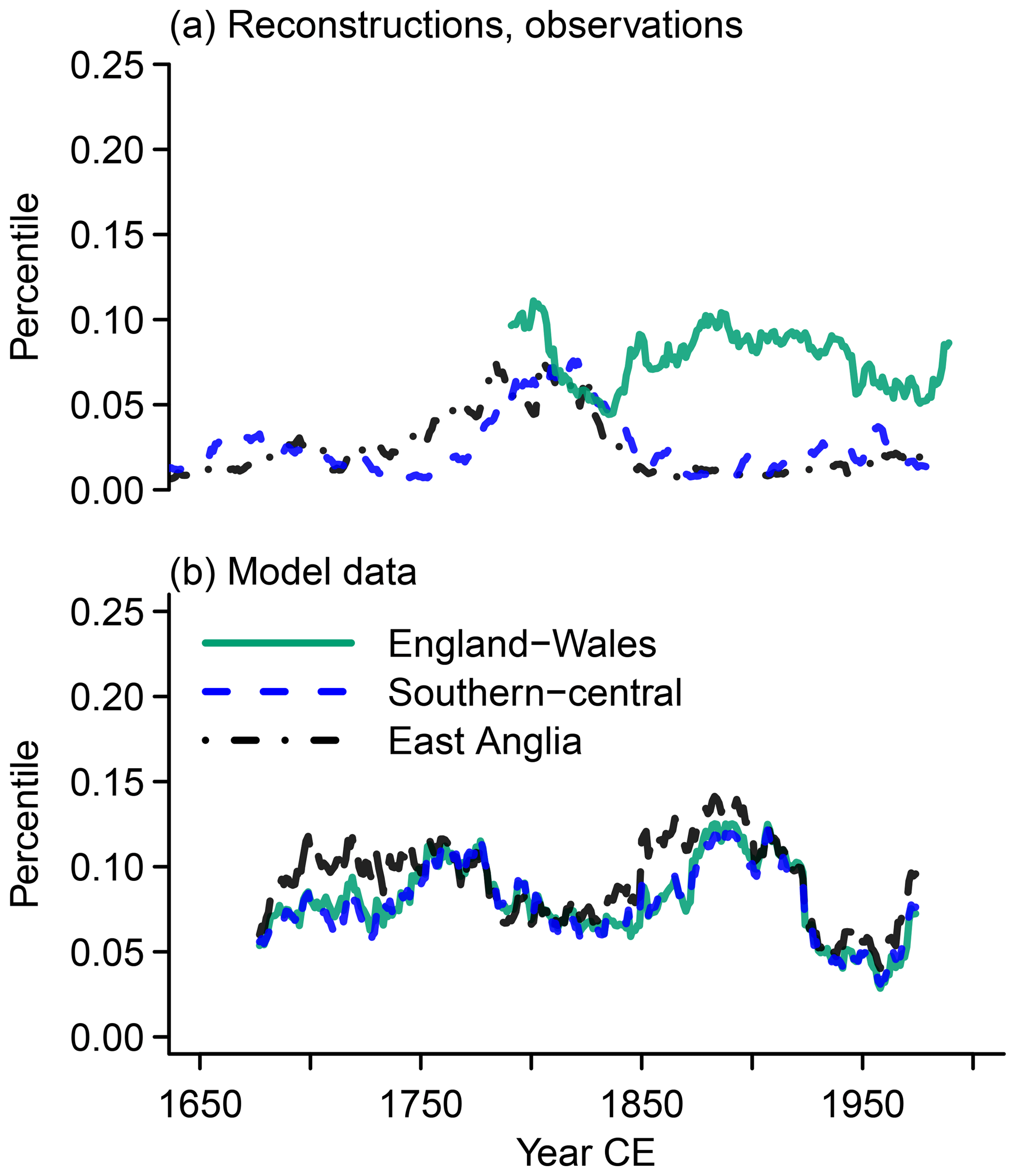
Figure 9 Visualization of how percentile values change over windows. We show what the percentile 6.7 MAMJJ precipitation amount for a reference window represents over time for England–Wales (green solid lines), southern–central England (blue dashed lines), and East Anglia (black dash-dotted lines) in (a) reconstructions, observations, and (b) simulations. The reference window is centered on 1815 CE.

In general, there are not any clear common evolutions between the different data sets before the 20th century. Only the dry percentiles in the simulation and the observations may evolve similarly in the period of their overlap (Fig. 9). Interestingly, there is an apparent contrast between the simulation output and reconstructions with potentially opposite evolutions in the period of their overlap prior to the 20th century in all shown series. In the 20th century, on the other hand, some commonalities may be inferred at least for the series representing the reference percentile 93.3 (Fig. 7).

Most prominent in these analyses is that the distributions for reconstructed precipitation show large shifts to larger precipitation amounts compared to the simulation and the observations. In contrast, the simulation and observations vary only within a rather narrow range. This may relate to the weaknesses of the reconstructions in representing not only low frequencies but also extremes (compare Cooper et al., 2013; Wilson et al., 2013). The regional simulation and the reconstructions again show an apparent opposite evolution for East Anglia and southern–central England. All sources of information tend to show shifts in the probability of precipitation amounts.

4.4 Relation between temperature and precipitation in different data sources

We briefly explore the interrelation between the regional temperature and precipitation variability focusing on the extended spring season from March to July. In particular, we show how interannual correlations between the precipitation records and temperature series evolve over time for this season.

Figure 10 plots sliding interannual correlations for 51-year windows between the observed and reconstructed precipitation data and the Central England Temperature data as well as the correlation between simulated England–Wales precipitation and simulated central England temperature. We plot correlations for the untransformed precipitation records. All records are for the MAMJJ season. Obviously, the large amount of internal variability on local and regional scales complicates the comparison among different data sources when studying such small regions.

We expect variability in moving correlation coefficients simply due to sampling variability (Gershunov et al., 2001). For example, a bootstrap procedure following Gershunov et al. (2001) suggests a 90 % credible interval for 51-year moving window correlations of between approximately −0.59 and approximately −0.21 for a correlation of approximately −0.43 between simulated central England temperature and England–Wales precipitation over the full period. That is, variations in Fig. 10 are probably within the sampling variability estimates for 51-year moving window correlations. That further implies that for overall uncorrelated data we can expect some windows to show statistically significant correlations. We do not show significance levels in Fig. 10 but we note that for 51-year windows and the time series characteristics of the data (e.g., approximately uncorrelated noise for seasonal precipitation), one may regard absolute values of correlation coefficients larger than 0.23 as statistically significant at the 5 % level.

On interannual timescales and over 51-year moving windows, all data sets evolve similarly in Fig. 10 for the extended spring season. However, observed and reconstructed data show weaker correlations in the late 20th century, while the correlation strength increases in the regional simulation. Both reconstructions show no statistically significant relation between temperature and precipitation over the full period. The reconstruction for East Anglia is intermittently negatively correlated with the temperature data. The observations show a notable negative relationship from the second half of the 19th to the mid-20th century. Only correlations between the regional simulation temperature and precipitation are negative and relatively strong (r≈0.5) throughout the full period.

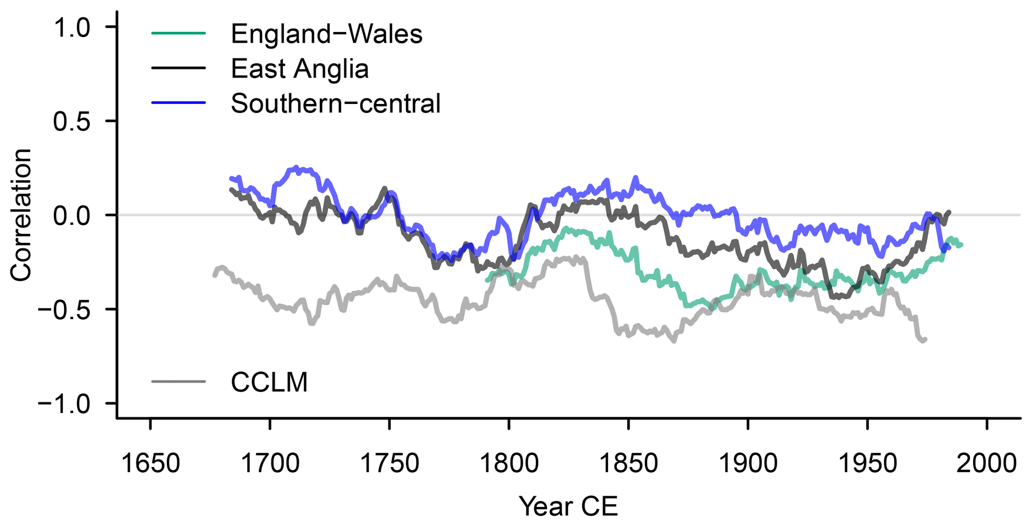
Figure 10 Interannual correlations over 51-year windows between extended spring (MAMJJ) Central England Temperature and various precipitation records: extended spring (MAMJJ) precipitation series for observational England–Wales precipitation (green), reconstructed East Anglia precipitation (black), and reconstructed southern–central England precipitation (blue). The grey line is for the simulated representations of the England–Wales MAMJJ precipitation and the central England temperature in MAMJJ.

The observed negative relation is well known. For example, Crhová and Holtanová (2018) show a slightly negative correlation between temperature and precipitation in observations over the southern British Isles in spring and summer. They also show that regional climate simulations usually capture this feature successfully.

4.5 Considering further reconstructions and global simulations

Here, we briefly describe additional results. If we perform similar analyses as described above but on a selection of the PMIP3 ensemble of global simulations (Schmidt et al., 2011), we do not find commonalities between the simulations or between the simulations and the other sources of information (not shown; see the Supplement). If we use different reconstructions, agreement between simulated and reconstructed precipitation does not necessarily increase, but differences between reconstructions and observations may be reduced (not shown; see the Supplement).

We use two different reconstructions based on δ¹⁸O. For one, we obtain the precipitation reconstruction by Rinne et al. (2013) for southern England for the May to August extended summer season. Secondly, we use the isotope records for England and Wales by Young et al. (2015) and scale the composite against the observational England–Wales precipitation data. We follow the procedure described by Young et al. (2015) but for two seasonal estimates, the extended spring from March to July used in our main analyses and, following Young et al. (2015), for the summer season from June to August.

The Supplement provides some details for our summer season scaling of the isotope data from Young et al. (2015). The most striking feature is again a notable difference in the percentiles prior to time windows approximately centered on the year 1850 compared to the later period. This feature resembles the behavior of the tree-ring-width-based reconstructions. While this may be due to the chosen calibration method and period, it appears more likely that there is a problem in the relationship between isotopes and precipitation for this early period.

Comparing our extended spring season scaling to the equivalent observations, there is limited agreement for the dry percentile after approximately the year 1850 (not shown) but otherwise we cannot find any consistency in these data compared to the observational counterparts. We also see no agreement between the data by Young et al. (2015) and the regional simulation output.

The period covered by the data from Rinne et al. (2013) only shortly overlaps the period of the observational data. For this overlap dry percentiles tend to agree with the observations but wet percentiles evolve oppositely (compare to the Supplement). The change in average precipitation for a reference year also agrees between the two data sets for the time of overlap (not shown). Compared to the regional simulation output, evolutions tend to be opposite.

If we consider the relation between temperature and precipitation in the additional data sets and their respective seasons, the disagreement between data sources changes compared to our main analyses (not shown). The observations show consistently negative correlations for the summer season, and the scaled isotope data by Young et al. (2015) agree quite well with the summer observations except for a large part of the 20th century when there is a markedly weaker negative correlation (not shown). The simulation again shows generally stronger correlations compared to the other data in summer and shows some agreement with the observations in the industrial period since approximately the year 1850 (not shown). If we correlate the scaled isotope data to the temperature for an extended spring season from March to July, the correlations are quite similar to those for the larger-domain simulation output but differ notably from the observations (not shown). The extended summer (MJJA) reconstruction by Rinne et al. (2013) agrees well with the respective observations by showing a consistently negative correlation (not shown). The relationship is weaker for the reconstruction prior to the period of the Oxford precipitation observations (not shown).

5 Discussion

5.1 Validity of approach

Information from reconstructions and from simulation output together increases our understanding of past climates. The PAGES Hydro2k Consortium (2017) made recommendations for valid and appropriate comparisons of hydroclimate data from both sources of information. Here, we consider approximately the last 350 years by comparing both estimates to long instrumental data. We have to consider whether our analyses are appropriate in the sense of the recommendations concerning uncertainties, the properties compared, and the expectations underlying the comparison (PAGES Hydro2k Consortium, 2017).

The observational England–Wales precipitation data are a weighted composite of regional series based on instrumental information. The information entering the composites and the regional index changed over time. Similarly, the reconstructions combine spatially distributed proxies, e.g., tree-ring-width series into regional-scale composite series (Cooper et al., 2013; Wilson et al., 2013), to maximize the common signal between different locations. On the other hand, the simulations are aggregations of various grid-point time series from the simulation output. We assume that the compositing and the aggregation have similar effects in removing local variability. In this respect, records from different sources are similar to each other and thus our comparison appears valid.

Explicit uncertainty estimates are only available for the reconstruction for East Anglia and only for a low-pass-filtered version of the data (Cooper et al., 2013). Our results as well as the discussions of Cooper et al. (2013), Wilson et al. (2013), Rinne et al. (2013), and Young et al. (2015) emphasize that uncertainties for the reconstructions are potentially large and that even the relationship to precipitation is not necessarily valid for some periods. Similarly, uncertainties affect the simulations not only with respect to our domain choice but also with respect to the algorithms and parameterizations implemented for simulating precipitation in the regional climate model.

Considering the limitations of any simulation and the known shortcomings of the reconstructions, questions may arise as to the validity and robustness of our analyses. Even if one assumes that prior discussions on the reconstructions invalidate their use, they would at least be a useful data source for our first goal of highlighting the benefits of adding the SPI to our set of tools for studying past precipitation variability.

However, we do not agree with such an assumption. The reconstructions are still, at least “preliminary” (as stated by Cooper et al., 2013), estimates of past precipitation for the southern British Isles. As such, it is of value to include them in a comparison of distributional precipitation characteristics between different data sources for this domain. It is further of interest to highlight for any available reconstruction on which properties the reconstructed precipitation distributions agree or disagree with the other sources of information. That is, understanding our sources of information about past climates requires the identification of their strengths as well as their shortcomings.

More generally, we argue that the transformation to standardized indices provides a sound basis for equivalence between the different precipitation estimates for subsequent comparisons of the distributional properties. Then, we assume that the comparison becomes informative for changes over time between these distributions. While we cannot expect accurate or even approximate temporal agreement between time series from simulation output and observation-based data on either interannual or multi-decadal timescales because of internal variability, the transformation makes our comparison one of climatologies. Furthermore, one may assume that the evolution of percentiles and variability may be more consistent between the different data sets than the average conditions.

5.2 Implications of the main results

Our analyses highlight the shortcomings of different reconstructions relative to observations. We also see that differences compared to observations may be comparable for reconstructions and simulations. Our approach further shows that apparently the reconstructions and the simulations occasionally evolve in opposite directions. This may signal that we indeed do not perform a valid comparison, that simulations may misrepresent forced responses, or, considering the relationship between the reconstructions and temperature, that the reconstructions do not fully reflect precipitation.

We expect disagreement between simulations and observations because of differing influences of internal variability (see discussion below). More critical is the lack of consistency between reconstructions and observations. Most notably, the reconstructions show unrealistically large changes in the cumulative probabilities represented by certain precipitation amounts for the extended spring season MAMJJ (compare Figs. 7 to 9). The reconstructions do not reliably represent the extended spring precipitation distributions in specific periods.

One result is the inconsistency of the relationships between temperature and precipitation in the data sets for the considered domains for the extended spring season. Tout (1987) and Crhová and Holtanová (2018) both note the negative relationship between temperature and precipitation observations for Britain. Tout (1987) does not find any changes in the negative relationship between England–Wales precipitation and Central England Temperature for the summer season from June to August between 1766 and 1980 CE. We only find the negative relationship for the extended spring consistently in the simulation and from approximately 1850 to 1950 CE in the observations. The tree-ring-width-based reconstructions do not show any clear relationship for the extended spring season. The disagreement between data sets changes for other seasons (not shown).

The differences between the simulation and observations may imply either shortcomings of any of the observational data sets in the early period or that the simulation presents a too-stable relationship between temperature and precipitation in southern Great Britain. Explanations might be physical inconsistencies within the simulations. More generally, any of the data sources may lack the physical relationship between the temperature and precipitation records in the chosen season. Another possibility is that internal large-scale climate factors influencing the relationship between the two parameters evolve differently in the simulation and reality. Assuming that the observations are the more reliable data set, we tend to infer that the disagreement between observations and reconstructions suggests major shortcomings in the reconstructions.

5.3 Internal vs. forced variability

If we expect temporal consistency among the different sources of information, then we are assuming that all the sources of information are responding to the impact of external climate forcing and that the regional simulation skillfully represents the climate response to these conditions. Nevertheless, internal climate variability may dominate even for large-amplitude exogenous forcing (compare, e.g., Deser et al., 2012a). We have to ask, what is our expectation of consistency between simulated and observed responses to exogenous influences?

The instrumental period overlaps the industrial period of anthropogenic climate forcing. Earlier exogenous forcing is potentially weak despite relatively large variations in solar activity (Clette et al., 2014) and the occurrence of a number of strong tropical volcanic eruptions during the period of interest (e.g., Schmidt et al., 2011).

Forced precipitation signals can agree in simulations, e.g., the CMIP5 21st century global projections (Fischer et al., 2014). A lack of an identifiable relationship to the forcing between different data sources in our study does not necessarily imply that the underlying climate data are wrong but may simply suggest that internal, e.g., oceanic, atmospheric, or coupled climate, variability masks, modulates, or counteracts an external forcing influence. That is, the lack of consistent evolutions points to shortcomings of the data sources or an overwhelming influence of internal variability. We have to emphasize that the regional simulation and its driving MPI-ESM-COSMOS simulation both use variations of the total solar irradiance forcing that could be unrealistically wide, and neither simulation includes a resolved stratosphere to account for potential UV-related top-down mechanisms (Anet et al., 2013, 2014).

In addition, our regional focus is close to the western boundary of the domain of the regional simulation, and thus we expect a rather strong influence of the dynamical evolution of the driving coarse-resolution simulation with MPI-ESM-COSMOS. Indeed, Blenkinsop and Fowler (2007) report a strong influence of the driving general circulation model on the representation of drought in regional climate simulations in southern Great Britain.

Relatedly, since the regional focus is a small domain, the influence of natural internal variability is likely large: in the case of the British Isles, variability in the North Atlantic Oscillation (Gómez-Navarro et al., 2012; Gómez-Navarro and Zorita, 2013; Hall and Hanna, 2018; Matthews et al., 2016). Thus, we should not expect simulations to agree with observations on the evolution of regional climate parameters and even an ensemble may show diverse behavior. Differences in internal variability between models, observations, and paleo-observations may include their representation of past changes in the relationship between the regional climate and the large-scale circulation (Pinto and Raible, 2012; Lehner et al., 2012; Raible et al., 2014).

Thus, while the forcing history suggests notable variations and the large-scale temperature records indicate an imprint of the forcing history on hemispheric and global temperatures, internal variability may dominate on smaller regional scales (e.g., Deser et al., 2012b). This is despite the fact that, e.g., the large-scale storm track is indeed sensitive to solar (e.g., Ineson et al., 2015) and volcanic forcing (e.g., Fischer et al., 2007; Trouet et al., 2018). Considering the possibly large role of internal variability on regional scales and the limitations of simulations in representing regional-scale precipitation, the occasionally consistent variations in precipitation distribution properties increase our confidence in simulated forced changes. However, while the regional simulation appears to present similar variations compared to the observations during some periods, we cannot say whether it does so for the right reasons.

6 Conclusions

This study pursued two goals. For one, we wanted to show that the Standardized Precipitation Index (SPI) over moving windows helps in the rigorous comparison of different sources of precipitation information over paleoclimatic timescales. The information on precipitation distributions obtained by the SPI approach eases a comparison of how different sources of information represent climatologies of precipitation. Second, by using this approach, we studied the consistency of the various sources of information for precipitation variations in a small regional domain in southern Great Britain.

Regarding the results for our specific study domain, first, we did not find any clear consistency for precipitation signals among a regional climate model simulation, an observational data set, and two local domain reconstructions. We conclude that the considered reconstructions appear to be unreliable representations of the observational series.

Second, the regional simulation shows occasional agreement with its observational target, the observational England–Wales precipitation data. In particular, the variability in both data sources shows comparable changes for the full period of the observations. This is possibly due to comparable changes in dryness, which also show some level of agreement over the full period. This partial agreement in terms of variability and dryness between the regional simulation and observations is encouraging. However, considering all associated uncertainties, we cannot conclude that the agreement in properties reflects agreement in the underlying processes in the respective data sources.

Third, the simulation data do not agree with the reconstructions. Nevertheless, an interesting result is the at times opposite evolution of the reconstructions and the regional simulations considering regional dryness and wetness, e.g., between 1750 and 1850. Again, considering all sources of uncertainty, we cannot attribute this to the external forcing or to errors in either data source.

Fourth, our data sources do not agree on the strength of the relationship between temperature and precipitation. However, the relationships between the two parameters share some common covariance on interannual timescales between the sources of information for the season from March to July, e.g., in the 19th century.

Generally, a dominant role of internal variability could explain the lack of consistency in standardized precipitation measures in the different data sets on the temporal and spatial scales we consider here; the relative role of the external climate forcing generally becomes weaker at smaller spatial and shorter temporal scales (Deser et al., 2012b). The lack of general consistency and slightly differing interannual relations between temperature and precipitation still require a closer look at the uncertainties in observations, the methods and input data for reconstructions, and dynamical and thermodynamical representations of regional climate in regional simulations.

Appendix A: Evaluation of the simulation setup against the CRU data

We shortly describe the performance of the COSMOS-MPI-ESM-CCLM setup compared to the observational CRU data (Harris et al., 2014; University of East Anglia Climatic Research Unit et al., 2017). We used version CRU TS 3.10, which has subsequently been superseded. The current version CRU TS 4.01 is available at http://doi.org/10/gcmcz3 (last access: 1 February 2019) with further information also given at https://crudata.uea.ac.uk/cru/data/hrg/ (last access: 20 September 2018).

The mean climate of the driving COSMOS-MPI-ESM simulation is too warm for much of the British Isles, the Scandinavian Alps, northern North Africa, Iberia, the Alps, southern France, Turkey, and Greece for all seasons over the period 1951–2000 (Fig. A1, top). It is generally too cold over the Baltic region, the eastern part of the model domain, the southern border of the domain over Africa, and central Europe. High-elevation and southern-area warm biases frequently exceed 6 K. Cold biases exceed 2 to 4 K occasionally over northeastern Europe and at the southern border of the domain. We attribute these biases to some extent to the cruder representation of the European orography and, possibly related to that, to biases in the modeled atmospheric circulation. However, the specific choice of forcings may also influence the climatology.

In the regional CCLM simulation (Fig. A1, bottom), warm biases for 1951–2000 are confined to the Atlas Mountains in all seasons and to the south of the domain in spring and summer. Cold biases are common otherwise and are largest over the northeast, frequently exceeding 3–4 K.

For precipitation, summer is frequently too dry in central Europe in COSMOS-MPI-ESM and especially at the west coast of Scotland and in the Alps (Fig. A2, top row). The southern domain is generally too dry in spring when Scandinavia is slightly too wet. Coastal and mountainous regions as well as Iberia, Italy, and southern France are more likely to be too dry in autumn and winter. Scandinavia is also too wet in autumn. The COSMOS-MPI-ESM winter climatology is too wet over much of central, eastern, and northern Europe.

In CCLM, too-dry conditions are generally confined to southern Europe and North Africa and areas affected by the storm track, i.e., the coasts of Scotland and Norway (Fig. A2, bottom row). They extend to southern–central Europe only in summer. The climate is too wet in Scandinavia and northeastern Europe in most seasons. Large parts of Europe are too wet in all seasons except summer. Noteworthy is the excess precipitation at the northern flank of the Alps from autumn to spring. Part of these discrepancies is possibly attributable to a too-zonal airflow outside the summer season.

In summarizing, the model presents a too-strong latitudinal temperature gradient over the European domain. The annual cycle of temperature is apparently too strong in the south with warm biases in summer but cold biases in winter and it is slightly too weak in the north with cold biases being stronger in summer than in winter. Similarly to temperature, the gradient in precipitation also appears to be too strong and the annual cycle amplitude differs between simulation and gridded observational estimates, especially for central Europe. Specifically, autumn and spring are wetter in the simulation, while summer conditions differ only slightly or are too dry, which implies a weaker annual cycle compared to observations.

Figure A1 (a) Difference between the driving MPI-ESM simulation and the CRU data for seasonal near-surface air temperature. (b) Difference for CCLM.

Figure A2 As Fig. A1 but for precipitation.

Appendix B: Uncertainty of running measures

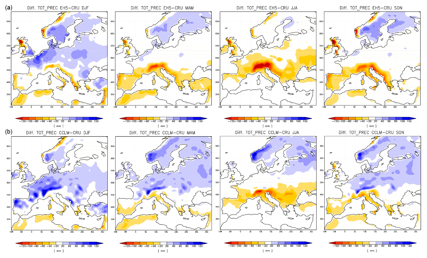
Figure B1 shows bootstrap estimates over 1000 40-year samples for each 51-year window. The estimates are for the running measures for reconstructions and observations for the three regions of interest (red) and the regional simulation (blue). The top row shows Weibull standard deviations and the bottom row is for the percentiles.

The figure highlights the fact that sampling variability is generally larger for the simulated data. Indeed, sampling variability may render differences between periods nonsignificant. However, the bootstrap distributions also appear strongly skewed.

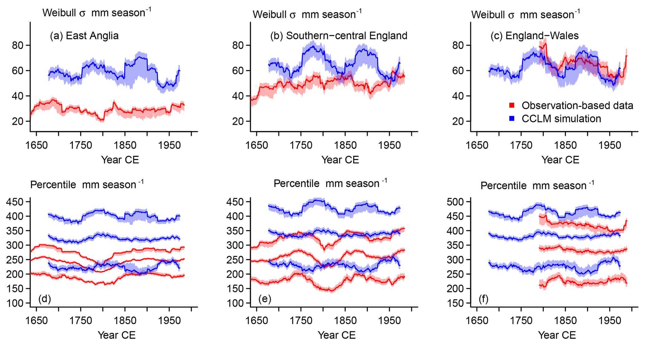
Figure B1 Visualization of uncertainty in the distributional properties. We use a bootstrap procedure on running estimates. We resample 40-year samples 1000 times from moving 51-year windows. Units are precipitation amounts. Shading represents 95 % intervals, lines are medians. (a, b, c) Weibull standard deviation. (d, e, f) Percentiles 93.3, 50, and 6.7. Red: reconstruction and observations. Blue: CCLM. (a, d) East Anglia, (b, e) southern–central England, and (c, f) England–Wales precipitation.

Appendix C: Distributional parameters

The Weibull distribution is a two-parameter distribution with a scale and a shape parameter. See, e.g., Sienz et al. (2012) for more details and how the distribution compares to other distributions in computing the Standardized Precipitation Index.

Figures C1 and C2 present the shape, k, and scale, λ, parameters of our Weibull distribution fits for the reconstructions for East Anglia and southern–central England, the observational England–Wales precipitation, and the respective time series in the simulation.

Results for the simulation show very similar evolutions among regions, highlighting the homogeneity of the simulation data. There are also similarities between the two reconstructions. One could argue the shape parameters evolve similarly in the observation and simulation.

The shape parameter determines the “shape” of the distribution. In our cases, changes in this parameter are rather small (compare Fig. C1). Nevertheless, they can result in notably different widths of distributions for a specific data set over time. It is interesting that there is only small overlap between the range of shape parameters for the East Anglia reconstruction and all other series.

Figure C1 Evolution of the shape parameter k for the Weibull distribution fits for the (a) East Anglia reconstruction, (b) southern–central England reconstruction, (c) England–Wales precipitation observational data, (d) East Anglia regional simulation, (e) southern–central England regional simulation, and (f) England–Wales precipitation regional simulation.

Larger-scale parameters for a constant shape parameter result in a flatter distribution that extends further to larger values. Smaller values result in a narrower distribution with a larger probability density at its peak.

The evolution of the shape parameter reflects, in our cases, the evolution of the skewness of the distributions (not shown). All distributions show negative skewness, and the amplitude increases with increases in the shape parameter.

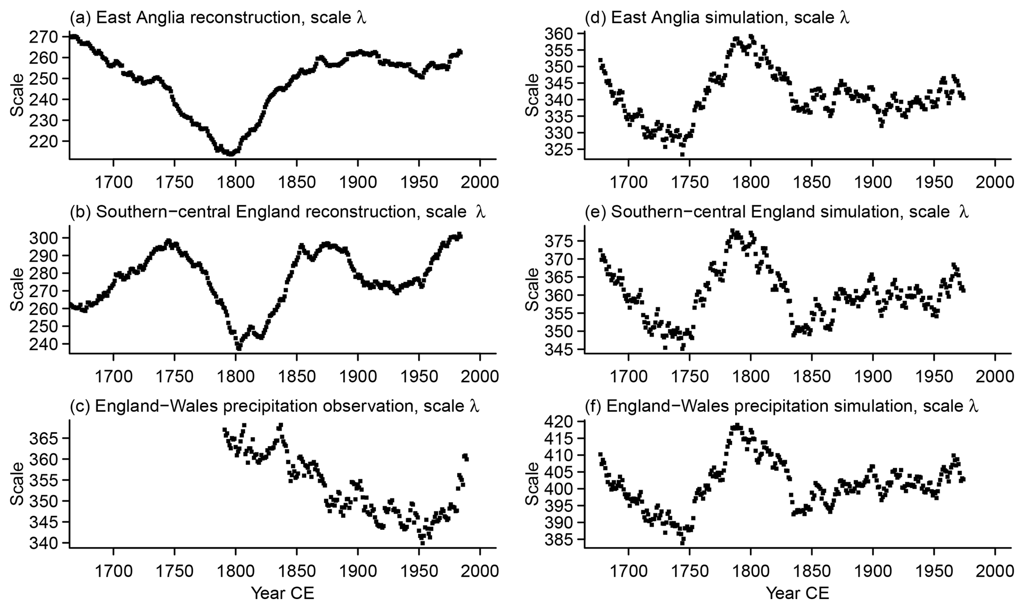
Figure C2 Evolution of the scale parameter λ for the Weibull distribution fits for the (a) East Anglia reconstruction, (b) southern–central England reconstruction, (c) England–Wales precipitation observational data, (d) East Anglia regional simulation, (e) southern–central England regional simulation, and (f) England–Wales precipitation regional simulation.

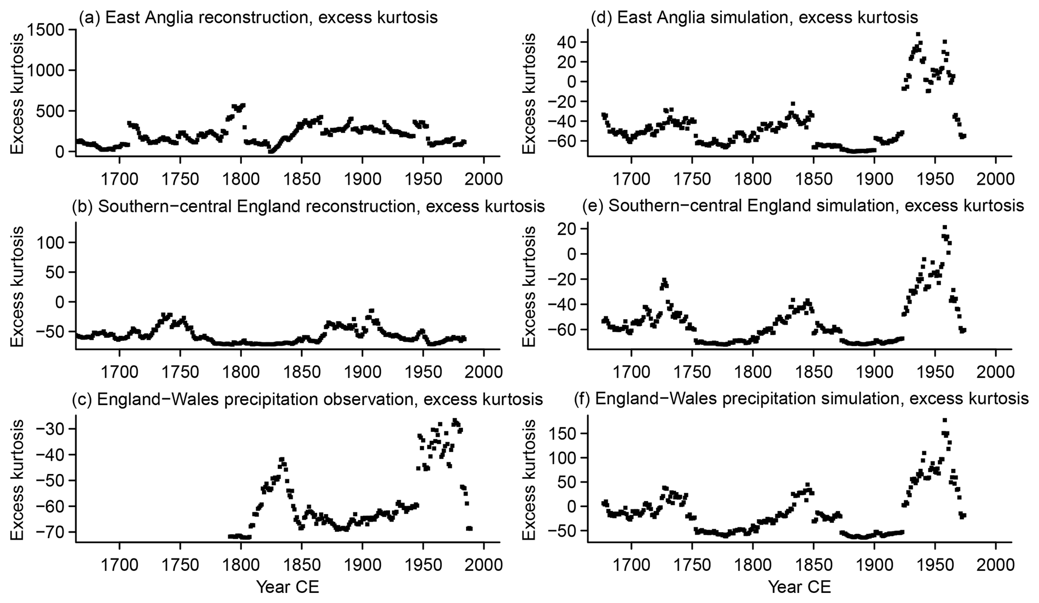
Figure C3 Evolution of the excess kurtosis of the fitted Weibull distributions for the (a) East Anglia reconstruction, (b) southern–central England reconstruction, (c) England–Wales precipitation observational data, (d) East Anglia regional simulation, (e) southern–central England regional simulation, and (f) England–Wales precipitation regional simulation.

Figure C3 shows the excess kurtosis over the period of interest. The most common feature for the different records is a negative excess kurtosis. Interestingly, the East Anglia reconstructions show large positive values. The simulation data have a period with positive, or for the simulated England–Wales precipitation larger positive, values in the middle of the 20th century, and the observed England–Wales precipitation shows only negative excess kurtosis. The scaling of the kurtosis axes for the reconstructions highlights the fact that they show much larger values earlier in the last millennium (not shown; compare to the Supplement).

Appendix D: External code

This paper uses a number of external software packages. File manipulations used Climate Data Operators (CDOs; https://code.mpimet.mpg.de/projects/cdo/, last access: 1 February 2019). Furthermore, the following R (R Core Team, 2018) packages helped in the work: gtools (Warnes et al., 2018), corrplot (Wei and Simko, 2017), ncdf (Pierce, 2015), VGAM (Yee, 2015), MASS (Venables and Ripley, 2002), nortest (Gross and Ligges, 2015), dplR (Bunn et al., 2018), zoo (Zeileis and Grothendieck, 2005), latex2exp (Meschiari, 2015), knitr (Xie, 2015), and rmarkdown (Allaire et al., 2018). RStudio (RStudio Team, 2016) was also essential. The paper was prepared using the rticles package (no reference available).

The SPI code is based on work by Frank Sienz (e.g., Sienz et al., 2012). Christian Zang provided a Gershunov bootstrap procedure (compare, e.g., Gershunov et al., 2001; Zang and Biondi, 2015) that we modified.