the Creative Commons Attribution 4.0 License.
the Creative Commons Attribution 4.0 License.
 | 14 Nov 2019
Water isotopes – climate relationships for the mid-Holocene and preindustrial period simulated with an isotope-enabled version of MPI-ESM
Alexandre Cauquoin
Martin Werner
Gerrit Lohmann
We present here the first results, for the preindustrial and mid-Holocene climatological periods, of the newly developed isotope-enhanced version of the fully coupled Earth system model MPI-ESM, called hereafter MPI-ESM-wiso. The water stable isotopes , and HDO have been implemented into all components of the coupled model setup. The mid-Holocene provides the opportunity to evaluate the model response to changes in the seasonal and latitudinal distribution of insolation induced by different orbital forcing conditions. The results of our equilibrium simulations allow us to evaluate the performance of the isotopic model in simulating the spatial and temporal variations of water isotopes in the different compartments of the hydrological system for warm climates. For the preindustrial climate, MPI-ESM-wiso reproduces very well the observed spatial distribution of the isotopic content in precipitation linked to the spatial variations in temperature and precipitation rate. We also find a good model–data agreement with the observed distribution of isotopic composition in surface seawater but a bias with the presence of surface seawater that is too 18O-depleted in the Arctic Ocean. All these results are improved compared to the previous model version ECHAM5/MPIOM. The spatial relationships of water isotopic composition with temperature, precipitation rate and salinity are consistent with observational data. For the preindustrial climate, the interannual relationships of water isotopes with temperature and salinity are globally lower than the spatial ones, consistent with previous studies. Simulated results under mid-Holocene conditions are in fair agreement with the isotopic measurements from ice cores and continental speleothems. MPI-ESM-wiso simulates a decrease in the isotopic composition of precipitation from North Africa to the Tibetan Plateau via India due to the enhanced monsoons during the mid-Holocene. Over Greenland, our simulation indicates a higher isotopic composition of precipitation linked to higher summer temperature and a reduction in sea ice, shown by positive isotope–temperature gradient. For the Antarctic continent, the model simulates lower isotopic values over the East Antarctic plateau, linked to the lower temperatures during the mid-Holocene period, while similar or higher isotopic values are modeled over the rest of the continent. While variations of isotopic contents in precipitation over West Antarctica between mid-Holocene and preindustrial periods are partly controlled by changes in temperature, the transport of relatively 18O-rich water vapor near the coast to the western ice core sites could play a role in the final isotopic composition. So, more caution has to be taken about the reconstruction of past temperature variations during warm periods over this area. The coupling of such a model with an ice sheet model or the use of a zoomed grid centered on this region could help to better describe the role of the water vapor transport and sea ice around West Antarctica. The reconstruction of past salinity through isotopic content in sea surface waters can be complicated for regions with strong ocean dynamics, variations in sea ice regimes or significant changes in freshwater budget, giving an extremely variable relationship between the isotopic content and salinity of ocean surface waters over small spatial scales. These complicating factors demonstrate the complexity of interpreting water isotopes as past climate signals of warm periods like the mid-Holocene. A systematic isotope model intercomparison study for further insights on the model dependency of these results would be beneficial.
- Article
(13948 KB) - Full-text XML
-
Supplement
(2921 KB) - BibTeX
- EndNote


The hydrogen and oxygen atoms that compose the water molecule have several natural stable isotopes. This results in several forms of the water molecule called water stable isotopologues (hereafter designated by the term “water isotopes”), the most common being , and HDO. These water isotopes, expressed hereafter in the usual δ notation (as δ18O and δD with respect to the Vienna Standard Mean Ocean Water V-SMOW if not stated otherwise), are integrated tracers of climatic processes occurring in diverse parts of the hydrological cycle (Craig and Gordon, 1965; Dansgaard, 1964). Because of their differences in mass and symmetry, an isotopic fractionation happens at each phase change depending on environmental conditions. As a consequence, the water isotopes have been successfully used during the last decades to study past climate changes and to describe the present-day water cycle through their measurements in various natural archives. Many of these studies are based on a modern analog approach, i.e., by assuming that the modern spatial relationship between water isotopes and surface temperatures, precipitation amount or salinity provides a calibration that can be used for different past climates. In addition, to be consistent with the observed close relationships between water isotopic time series and temperature or precipitation amount variations, this hypothesis can be validated by a Rayleigh distillation model representing the evolution of the remaining water vapor in a cloud (i.e., loss of heavier isotopes during condensation and precipitation events) as it is transported from moisture source region to high latitudes (Ciais and Jouzel, 1994). For example, the isotopic signal measured in polar ice cores enabled at a 1st order the reconstruction of past temperature variations at high resolution (Jouzel, 2013, and references therein), allowing for the description of past climate changes over several glacial–interglacial periods (Jouzel et al., 2007; NEEM Community Members, 2013). In the (sub)tropical areas, the δ18O in the calcite of speleothems is interpreted in terms of past monsoon dynamics (i.e., linked to the quantity of precipitation, called the “amount effect”) (Wang et al., 2001, 2008). Analogously to the continental speleothems, the δ18O conserved in the carbonates of foraminifers or corals can be measured. It is controlled by the 18O isotopic composition of ocean water and the temperature at the calcite formation. Such records from marine sediment cores are essential to deduce mean sea level changes, which are linked to the global ice volume during different climates (Shackleton, 1967). Moreover, the local variations in the δ18O of ocean water tend to be dependent on changes in freshwater budget and ocean circulation, so they provide information about salinity changes. Finally, the combination of δD and δ18O measured in the same sample gives access to the 2nd-order parameter deuterium excess (d-excess), defined as d-excess =δD δ18O (Dansgaard, 1964). Deuterium-excess changes are often interpreted as a source region effect; i.e., d-excess is related to the humidity and temperature conditions at the evaporative source regions (Merlivat and Jouzel, 1979). Other processes that could drive the d-excess variability have been suggested, like the moisture source relative humidity (Pfahl and Sodemann, 2014), the moisture recycling or the evaporation of falling drops (Fröhlich et al., 2002).
However, the quantitative translation of past isotope signals recorded in natural archives to climate variables and their interpretation remains challenging because of the numerous and complex processes involved: changes in evaporation conditions and moisture sources, in atmospheric transport pathways, or in the seasonality of the precipitation. For example, using the spatial relationship between the δ18O in Greenland ice core records and surface temperature to evaluate the local temperature variations during the last deglaciation leads to a large uncertainty of a factor of 2 (Jouzel, 1999; Buizert et al., 2014). This has been attributed to changes in air mass origins (Werner et al., 2001), precipitation seasonality (Krinner et al., 1997; Krinner and Werner, 2003) or to a dampening of isotopic changes by ocean evaporation (Lee et al., 2008). In East Antarctica, it has been suggested that the relationship between temperature and the isotopic signature for warmer interglacial periods can vary among ice core sites, with an error on the temperature reconstruction that can reach up to 100 % (Sime et al., 2009; Cauquoin et al., 2015). At lower latitudes, the interpretation of water isotope records is even more complex because of the convective processes (Risi et al., 2008) and the importance of the precipitation intensity that affect the isotopic composition of these records (Vimeux et al., 2005). In the oceans, quantitative reconstructions of past salinity variability based on its spatial relationship with δ18O in ocean water may have very large errors and uncertainties, too (LeGrande and Schmidt, 2011).
One way to improve our understanding of the mechanisms controlling the water isotope distribution linked to the variations of climate is to use general circulation models (GCMs) with explicit diagnostics of water stable isotopes. These complex models consider the numerous physical processes that influence the isotopic composition of the different water bodies in the Earth's climate system. Since the pioneering work of Joussaume et al. (1984), several isotope-enabled GCMs have been built both for the atmosphere (Jouzel et al., 1987; Hoffmann et al., 1998; Mathieu et al., 2002; Noone and Simmonds, 2002; Schmidt et al., 2005; Lee et al., 2007; Yoshimura et al., 2008; Risi et al., 2010b; Werner et al., 2011; Kurita et al., 2011; Nusbaumer et al., 2017) and the ocean (Schmidt, 1998; Paul et al., 1999; Delaygue et al., 2000; Xu et al., 2012; Liu et al., 2014). These models are extremely powerful because they make it possible to perform direct comparisons, at different time periods, with environmental proxy records and to reduce the uncertainties resulting from the interpretation of these records in terms of climate signals in model–data comparisons. They have been used for a considerable range of applications: e.g., analyses of mixing processes within rain events (Risi et al., 2010a), an estimation of the changes in temperature and ice sheet height in Antarctica during the last glacial period (Werner et al., 2018), and a study of the link between oceanic water isotopic content and salinity, which is of crucial interest in paleoceanography (Delaygue et al., 2000).
When simulating different climates or evolving climate conditions, it is essential to describe in a coherent way the numerous links and feedbacks between the different natural reservoirs (atmosphere, land–vegetation, ocean) and to minimize the prescription of unknown boundary conditions (e.g., sea surface temperatures). For paleoclimate isotope applications, it means that it is necessary to simulate the water isotopes in a full hydrological cycle system, not only in the atmosphere or in the ocean components. With the gain in performance of supercomputers, it is now possible to model the water isotopes in fully coupled atmosphere–ocean GCMs. In the past decade, such models have been used to examine the internal variability and the forced response to orbital and greenhouse gas forcing for modern and mid-Holocene (6 ka) climates (Goddard Institute for Space Studies (GISS) ModelE: Schmidt et al., 2007) and to study the isotopic signature of the El Ninõ–Southern Oscillation linked to the tropical amount effect (Hadley Centre Coupled Model, version 3 (HadCM3): Tindall et al., 2009). This same model has been used to investigate the 8.2 ka event by performing freshwater hosing experiments (Tindall and Valdes, 2011), allowing for model–data comparisons with paleo-isotope observations from lake sediments (Holmes et al., 2016). More recently, the isotopic-enabled model HadCM3 has been used to reconstruct past paleosalinity from modeled δ18O in ocean water during the modern period, the Last Glacial Maximum (LGM, 21 ka) and the last interglacial optimum (LIG, 130 to 115 ka) (Holloway et al., 2016), as well as to investigate the magnitude of Antarctic warming in response to Northern Hemisphere meltwater input at 128 ka (Holloway et al., 2018). With the same model, Sime et al. (2019) confirm the primary importance of sea ice as a control on southern Greenland ice core δ18O during Dansgaard–Oeschger events. Using the ECHAM5/MPIOM model, Werner et al. (2016) have examined the changes in δ18O and d-excess between the LGM and the modern period. This same model has been exploited to examine the δ18O–temperature temporal relationship between the LIG and the modern period (Gierz et al., 2017).
The mid-Holocene (6k) is one of the PMIP4–CMIP6 (Paleoclimate Modeling Intercomparison Project – Coupled Model Intercomparison Project) past climates to evaluate the performance of the coupled GCMs (Kageyama et al., 2018). The mid-Holocene climate provides the opportunity to evaluate the model response to changes in the seasonal and latitudinal distribution of insolation induced by different orbital parameters. Due to a larger obliquity 6000 years ago and changes in the precession (Berger, 1978), the amplitude of the seasonal changes in insolation is amplified in the Northern Hemisphere according to the increase in boreal summer insolation and the decrease in boreal winter insolation. This is the opposite for the Southern Hemisphere. So, the mid-Holocene is characterized by an enhanced seasonal contrast in the Northern Hemisphere, with warmer summers in this part of the Earth, and by a strengthening of the African, Indian and Asian monsoons. Even if the forcing mechanisms are not linked to anthropogenic actions, a better quantification of the contributions of the orbital forcing variations and their related feedbacks on large-scale climate variations, like the amplification in seasonal temperature changes and the related responses of the hydrological cycle and of the oceanic circulation, is still an important issue that is relevant for evaluating future climate projections. A good way to progress on these questions is to investigate the variability of the isotope-to-climate gradients (spatial and temporal) for warm climatic periods under different orbital forcing conditions like PI and 6k.
In this paper, we present the first results of a new isotope-enhanced version of the fully coupled Max Planck Institute for Meteorology Earth System Model (MPI-ESM) (Giorgetta et al., 2013; Mauritsen et al., 2019), called hereafter MPI-ESM-wiso. It follows the efforts of Werner et al. (2016), who developed the previous model version. The better performance of presently available supercomputers combined with an optimization of the computational cost of the model allow us to run MPI-ESM-wiso with a finer spatial horizontal resolution compared to other isotope-enabled fully coupled models (e.g., the horizontal resolution is 2 times better than for the ECHAM5/MPIOM model setup used by Werner et al., 2016). Our study focuses on isotope changes and isotope–climate relationships for the mid-Holocene and preindustrial period. The outline of the paper is as follows. In Sect. 2, we briefly describe the model components, the implementation of water isotopes and the dataset used for model evaluation. In Sect. 3, we evaluate MPI-ESM-wiso simulation results. We present the simulated spatial variations of water isotopes in the atmospheric and oceanic compartments for both the preindustrial and mid-Holocene periods and compare them with available observations. We also analyze their spatial relationships with climate variables like near-surface air temperature and ocean salinity. In Sect. 4, the temporal relationships between water isotopes and climate variables are analyzed during and between the mid-Holocene and preindustrial periods. We conclude the article with a summary of our findings and some remarks in Sect. 5.
2.1 MPI-ESM-wiso
For this study, we have implemented the water stable isotopes in the Earth system model MPI-ESM (Giorgetta et al., 2013; Mauritsen et al., 2019) version 1.2.01p1. It consists of the components ECHAM6 (Stevens et al., 2013) for the atmosphere, MPIOM (Jungclaus et al., 2013) for the ocean, JSBACH (Reick et al., 2013; Schneck et al., 2013) for the land and vegetation, and HAMOCC (Ilyina et al., 2013) for the marine biogeochemistry. The coupling of atmosphere and land processes on the one hand and physical ocean and biogeochemistry on the other hand is done by the OASIS3 coupler (Valcke, 2013). MPI-ESM has been used for a wide range of CMIP5 experiments and will participate in CMIP6/PMIP4 with different model configurations (i.e., resolutions) and experiments (Eyring et al., 2016; Kageyama et al., 2018).
To explicitly simulate both and HDO within the different parts of the hydrological cycle, MPI-ESM has been equipped with water isotope diagnostics in each of its components in the same way as in the previous model version (ECHAM5, JSBACH, MPIOM) (Werner et al., 2016). Here, we give a brief summary of key model components, including their differences from the previous model setup and the isotope implementation within them. As the physical and dynamical processes in the water cycle are only involved in the ECHAM6, JSBACH and MPIOM components, we do not consider HAMOCC in the following descriptions.
The atmospheric general circulation model ECHAM6 has been developed on the basis of ECHAM5 (Roeckner et al., 2003). A detailed description of the model is given by Stevens et al. (2013). ECHAM6 consists of a dry spectral-transform dynamical core, a transport model for scalar quantities other than temperature and surface pressure, a suite of physical parameterizations for the representation of diabatic processes, and boundary datasets for externalized parameters (trace gas and aerosol distributions, land surface properties, etc.) (Stevens et al., 2013). The most important differences between ECHAM5 and ECHAM6 concern the radiation schemes with an improved representation of radiative transfer in the solar part of the spectrum, the computation of surface albedo, a new aerosol climatology and an improved representation of the middle atmosphere. Moreover, minor changes have been made in the representation of convective processes and through the choice of a slightly different vertical discretization within the troposphere. As in ECHAM5, the water cycle in ECHAM6 contains formulations for the evapotranspiration of terrestrial water, the evaporation of ocean water, and the formation of large-scale and convective clouds. Within the atmosphere's advection scheme, vapor, liquid and frozen water are transported independently. The water stable isotopes , and HDO have been explicitly implemented into the hydrological cycle of ECHAM6 in an analogous manner to the previous model release ECHAM5 (Werner et al., 2011). The water isotopes are implemented parallel to the “normal” water cycle: the isotopes are described identically as the normal water as long as no phase transitions are concerned. Additional fractionation processes are defined for the water isotope variables whenever a phase change of the normal water occurs. The equilibrium fractionation coefficients between vapor and liquid–ice water are calculated from Merlivat and Nief (1967) and Majoube (1971a, b). The kinetic (i.e., nonequilibrium) effects during evaporation from ocean sea surface and snow formation follow the formulations of Merlivat and Jouzel (1979) and Jouzel and Merlivat (1984), respectively. For the latter, we use the same supersaturation function as Werner et al. (2011). In the coupled setup, ECHAM6 provides the required freshwater flux (net precipitation P−E) and its isotopic composition for all ocean grid cells to the MPIOM ocean model.
The land surface model JSBACH (Reick et al., 2013; Schneck et al., 2013) calculates the boundary conditions for ECHAM6 over terrestrial areas. It simulates water-, energy- and carbon-related processes including interactive and dynamic vegetation, which is controlled by the processes of natural growing and mortality, as well as disturbance mortality (e.g., wind, fire) (Brovkin et al., 2009; Reick et al., 2013). The physical processes partitioning water masses on the land surfaces comprise the separation of rainfall and snowmelt into surface runoff and infiltration as well as the calculation of lateral drainage. Contrary to the previous release of JSBACH, the soil hydrology is now simulated similarly to the soil temperatures within five soil layers (Hagemann and Stacke, 2015) with increasing thickness (0.065, 0.254, 0.913, 2.902 and 5.7 m), the lower boundary being at almost 10 m of depth. The isotopic processes are represented in the same way as described in Werner et al. (2016); i.e., the water isotopes are passive tracers in the JSBACH model. No fractionation of the isotopes is assumed during most physical processes partitioning water masses on the land surface: the surface runoff has the isotopic composition of the rainfall and snowmelt that reach the soil surface, and drainage has the isotopic composition of soil-layer water (Haese et al., 2013). The water that percolates by gravitational drainage from one soil layer z to the layer below z+1 has the isotopic composition of moisture content in the layer z. The transport of , and HDO between the different layers via the vertical diffusion is treated in the same way as for the standard water. For evapotranspiration, the fractionation of isotopes might occur during the evaporation of water from bare soils (i.e., from the surface soil layer). However, the strength of this fractionation remains an open question. In accordance with the results of Haese et al. (2013) and as explained by Werner et al. (2016), we assume in this study that we can ignore any possible fractionation during evapotranspiration processes from terrestrial areas, as our analyses will focus primarily on the isotopic composition of precipitation.
As a part of the coupled model MPI-ESM, the Hydrological Discharge (HD) model (Hagemann and Gates, 2003) globally simulates the lateral freshwater fluxes at the land surface that go to the ocean at a daily time step. Modeled water discharge is calculated with respect to the topography gradient between grid boxes, the slope within a grid box, the grid box length, the lake area and the wetland fraction of a particular grid box. For the simulated total river runoff, it is assumed that the global water cycle is closed, i.e., that all net precipitation (P−E) over terrestrial areas is transported to the ocean. As MPI-ESM does not include a dynamic ice sheet model, precipitation amounts falling on glaciers are instantaneously put as runoff into the nearest ocean grid cell to close the global water budget. The HD model computes the discharge at 0.5∘ horizontal resolution. The model input fields for runoff and drainage resulting from the ECHAM6 resolution (such as T63 in this study) are therefore interpolated to the same 0.5∘ grid. Water stable isotopes are incorporated as passive tracers within the HD scheme.
The ocean component, MPIOM, has remained unchanged, except for the adaptations to high-resolution grids (Jungclaus et al., 2013). MPIOM is a free-surface ocean general circulation model formulated on an Arakawa-C grid in the horizontal and a z grid in the vertical. It contains subgrid-scale parameterizations for convection, vertical and isopycnal diffusivity, horizontal and vertical viscosity, and the bottom boundary layer flow across steep topography. MPIOM includes a sea ice model formulated using the viscous–plastic rheology of Hibler (1979). Sea ice thermodynamics relate changes in sea ice thickness to a balance of radiant and turbulent atmospheric fluxes, as well as oceanic heat fluxes. The effect of snow accumulation on sea ice is included, along with snow–ice transformation. As in the previous model version (Xu et al., 2012; Werner et al., 2016), , and HDO are treated as conservative passive tracers within MPIOM. The isotopic variations occurring in this component depend on oceanic advection and mixing of different water masses, on the isotopic composition of freshwater fluxes entering in the ocean (P−E and runoff discharge), and on the temperature-dependent isotope fractionation during evaporation. The isotopic composition of sea ice, formed from liquid waters, is also calculated by a liquid-to-ice equilibrium fractionation factor of 1.003, which is the average from various estimates (Craig and Gordon, 1965; Lehmann and Siegenthaler, 1991; Macdonald et al., 1995; Majoube, 1971a). Due to the very low rate of isotopic diffusion in sea ice, we assume no fractionation during sea ice melting. In a coupled setup, MPIOM provides the isotopic composition of ocean surface water and sea ice as boundary conditions to the ECHAM6 atmosphere model.
The coupling procedure between the atmosphere and the ocean in MPI-ESM, via the OASIS3 coupler (Valcke, 2013), has remained unchanged compared to the ECHAM5/MPIOM model setup. Mass, energy and momentum fluxes, as well as the related isotope masses of , and HDO, are exchanged between the atmosphere and ocean once per day.
2.2 Model setup and experiments
For this study, we have used the MPI-ESM-LR configuration (LR is for low resolution). The atmospheric component ECHAM6 was run at an approximately 1.875∘ horizontal resolution with 47 vertical pressure levels extending to 0.01 hPa (T63L47), while the previous T31L19 grid of ECHAM5 used by Werner et al. (2016) had a 3.75∘ horizontal resolution and the 19 vertical levels extended to 10 hPa. The same horizontal resolution is applied for the JSBACH land surface scheme. For the ocean component MPIOM, a bipolar grid with 1.5∘ horizontal resolution (near the Equator) and 40 z levels has been used (GR15L40). The poles of the ocean model are moved to Greenland and to the coast of the Weddell Sea by a conformal mapping of the geographical grid. Again, the horizontal resolution is finer than the 3∘ resolution (GR30L40) used in Werner et al. (2016).
Two different experiments were performed: one for the preindustrial period (PI) corresponding to the climate conditions at 1850 CE and one for the mid-Holocene 6000 years ago (6k). For the preindustrial climate, MPI-ESM has been continued from a standard PI simulation, i.e., without isotopes included, which has been run over 1000 years (Christian Stepanek, personal communication, 2019) using identical PI boundary conditions. In an analogous way as Werner et al. (2016), water isotope values in the atmosphere were initialized with constant values: δ18O and δD . For the isotope distribution within MPIOM-wiso, we have decided to start with constant concentration values of the passive tracers , and HDO in such a way that the respective δ18O and δD in the ocean are both at 0 ‰ (Baertschi, 1976; de Wit et al., 1980). The fully coupled MPI-ESM-wiso with isotope diagnostics was then run under PI conditions according to the PMIP4 protocol (orbital forcing, greenhouse gas concentrations, ocean bathymetry, land surface and ice sheet topography) for 2500 years. The 6k simulation is as the PI one but with the mid-Holocene orbital and radiative active trace gas forcing according to the PMIP4 experimental design (Table 1 of Otto-Bliesner et al., 2017). Again, our isotopic simulation for 6k has been continued from a 1000-year-long mid-Holocene simulation without isotopes (Christian Stepanek, personal communication, 2019). The water isotope values have been initialized in the exact same way as for the PI simulation, and MPI-ESM-wiso was then run for an additional 2500 years.
At the end of the simulations, the global mean 2000 m deep salinity changes by less than 0.002 practical salinity units (psu) over 100 years, and the globally averaged δ18O signature at 2000 m of depth changes by less than 0.002 ‰ per 100 years. Thus, we consider both simulations to be quasi-equilibrated and use the last 150 model years for our analyses. If not stated otherwise, all δ values of meteoric waters are calculated as a precipitation-weighted mean with respect to the V-SMOW scale. The δ values of ocean values are calculated as arithmetic averages, also with respect to the V-SMOW scale.
2.3 Observational data
To evaluate our model, we used different datasets including isotopic measurements in precipitation, ocean water, ice cores and continental speleothems. We give a brief summary below.
For the modern isotopic content of precipitation, we use the Global Network of Isotopes in Precipitation (GNIP) database, available through the International Atomic Energy Agency (IAEA), whose measurements began in the early 1960s. While several stations were monitored continuously for the isotopic content of precipitation throughout several decades (e.g., Vienna station), other GNIP stations stopped their operation after a shorter period. This is why we use in this study a subset of 70 stations from this database, for which surface temperature, precipitation rate, δ18O and δD have been measured for at least 5 calendar years within the period 1961 to 2007. Performing a preindustrial simulation instead of a present-day one, which is a slightly warmer climate, probably adds a negative bias in our modeled temperatures, and therefore in the modeled isotopic composition, compared to the GNIP observations. However, we do not expect a significant change in the relationships between water isotopes and temperatures (or precipitation) because the PI and present-day climates remain globally similar.
To evaluate the modeled PI isotope values in the ocean, we use the Goddard Institute for Space Studies (GISS) global seawater oxygen-18 database (Schmidt et al., 1999), which is a collection of over 26 000 seawater 18O values. We are using only the values with no applied corrections (see details in Schmidt et al., 1999). As the GISS δ18O in ocean water (δ18Ooce) values do not represent annual mean values but measurements on an arbitrary day of the year, we compare them to the simulated long-term mean monthly value of the sampling month when it is specified in the GISS database. We focus only on the near-surface δ18Ooce values between 0 and 10 m of depth in this study. Even if the GISS data are not preindustrial observations, we do not expect a significant increase in the bias in our modeled salinity and isotopic values because of the inertia of the ocean system.
Since the pioneering work of Dansgaard et al. (1969), Lorius et al. (1979) and others, analysis of the isotopic composition of polar ice cores has provided a lot of information about the climate of the past. We use here 5 Greenland and 10 Antarctic ice cores, selected from the comprehensive compilations of Sundqvist et al. (2014) and WAIS Divide Project Members (2013), to compare the measured isotopic values for the preindustrial climate with our model results. When available, we also report the 6k−PI differences in δ18O. We take for PI the values averaged over the last 200 years and for 6k the average in the 6±0.5 ka period. The ice core data used in this study are summarized in Table 1. We also add to this ice core dataset the 6k−PI δ18O anomalies measured from four (sub)tropical ice cores (Huascaran, Sajama, Illimani and Guliaa ice cores), which are reported in Table 3 of Risi et al. (2010b).
Table 1Selected ice core records and their geographical coordinates, reported PI values of δ18O and d-excess, and changes in δ18O and d-excess between 6k and PI. All values are given with respect to the V-SMOW scale.
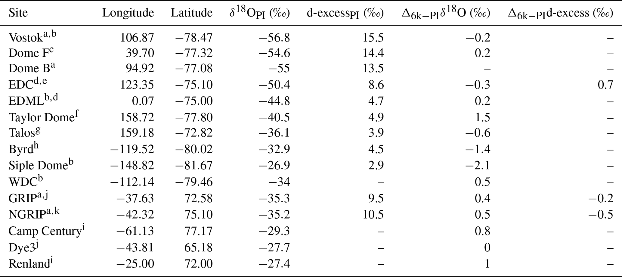
References: a reported in Risi et al. (2010b), b WAIS Divide Project Members (2013), c Kawamura et al. (2007), d Stenni et al. (2010), e Landais et al. (2015), f Steig et al. (2000), g Stenni et al. (2011), h Blunier and Brook (2001), i Vinther et al. (2009), j Vinther et al. (2006), k North Greenland Ice Core Project members (2004).
Furthermore, we also use the SISAL (Speleothem Isotope Synthesis and Analysis) dataset (version 1b: Atsawawaranunt et al., 2019), updated recently by Comas-Bru et al. (2019). It provides isotope records, including δ18O, from 455 speleothems from 211 cave sites. For our study, we have followed the recommendation of Comas-Bru et al. (2019) by selecting 30 speleothem sites (33 cores) for which averaged δ18O values are available for both the mid-Holocene (defined as the period 6000±500 years BP) and preindustrial periods (defined as the interval 1850–1990 CE). Using this extended modern baseline for the PI values increases the data uncertainties by only ±0.5 ‰ (Comas-Bru et al., 2019). Moreover, our selected PI base period is still more restricted than the one used by Werner et al. (2016), who selected the last 1000 years, which allows us to reduce the uncertainties without substantially decreasing the available number of mean δ18O speleothem values for both periods. Concerning the possible biases in the model–data comparison, a seasonal bias can appear in the isotopic composition of drip water archived in a speleothem record due to the re-evaporation of the precipitated water (Wackerbarth et al., 2010). An additional fractionation between the drip water and the formed calcite can also be observed for many speleothems (Dreybrodt and Scholz, 2011). The δ18O in speleothem calcites (δ18Oc) is expressed with respect to the Pee Dee Belemnite (PDB) standard. To directly compare these data with our model results (δ18O in precipitation: δ18Op), we first need to convert the δ18O values in calcite between the PDB and the SMOW scale (Coplen et al., 1983) using
and then apply a formula linking δ18O in water (δ18Owater(SMOW)) and δ18O in speleothem calcite (Tremaine et al., 2011):
with T being the temperature in Kelvin during calcite formation. To convert the speleothem PI values of δ18Oc in calcite to δ18Op in precipitation, we have determined the required site temperatures by interpolating annual mean ERA40 soil temperatures (layer no. 1, mean of the period 1961–1990) to the different speleothem sites. For the direct model–data comparison of the 6k−PI δ18O changes, we use both the simulated 6k−PI temperature and δ18Op changes to calculate the modeled change in δ18Oc in calcite.
3.1 Evaluation of MPI-ESM-wiso under PI conditions
3.1.1 Water isotopes in precipitation
Figure 1a shows the global distribution of the simulated annual mean δ18Op values in precipitation. The main well-known patterns of the global δ18Op distribution can be found in the model. They are very similar to those already observed with ECHAM5/MPIOM (Werner et al., 2016) and in agreement with present-day observations (circles: GNIP, squares: ice cores, triangles: speleothems). Typically, enhanced 18O-depleted precipitation with decreasing temperature (temperature effect) and increased altitude (altitude effect) is well simulated by MPI-ESM-wiso. The lowest simulated values of δ18Op occur over the polar regions, with the minimum value over East Antarctica (−54.5 ‰). A decrease in δ18Op is also observed going inland (continental effect) and with increased precipitation intensity over the low latitudes (precipitation amount effect).
In Fig. 1b, we compare our modeled δ18Op with the observational dataset described in Sect. 2.3. The speleothem PI values of δ18Oc in calcite are converted to δ18Op in precipitation by using Eqs. (1) and (2). The modeled δ18Op values are in very good agreement with the observations, with a linear regression gradient of 0.87 (1.0 being the perfect fit) and a root mean square error (RMSE) of 2.3 ‰. This represents an improvement compared to the modeled results from ECHAM5/MPIOM (RMSE of 3 ‰; Werner et al., 2016). The modeled global δ18Op–temperature relationship (for temperature below 20 ∘C; Fig. 1c) is also improved with a gradient 0.63 ‰ ∘C−1 (r2=0.97), very close to the observed one (0.66 ‰ ∘C−1, r2=0.95). This improvement, compared to the results from Werner et al. (2016), is mainly due to a better model–data agreement for the very low temperatures over the poles, which constitute an extreme test for isotope-enabled GCMs. This is confirmed by the good agreement of our modeled δ18Op–temperature spatial gradient over Antarctica (0.71 ‰ ∘C−1, r2=0.97) with the gradient of 0.8 ‰ ∘C−1 deduced from the Antarctic isotopic observations compiled by Masson-Delmotte et al. (2008). However, even if the warm bias for the coldest temperatures over Antarctica is reduced, the modeled δ18Op values are still too high at these locations (Fig. 1b). Concerning the δ18Op–precipitation spatial gradient, we calculate observed and modeled values of −0.47 and −0.36 ‰ mm−1 d, respectively, for the nine low-latitude GNIP stations with an annual mean temperature equal or above 20 ∘C. These results have to be taken with caution because of the few available tropical GNIP station records. The rather large standard errors of the gradients, estimated by using the variance–covariance matrix between the regression coefficients, illustrate this point well (0.165 and 0.145 ‰ mm−1 d for GNIP and MPI-ESM-wiso results, respectively).
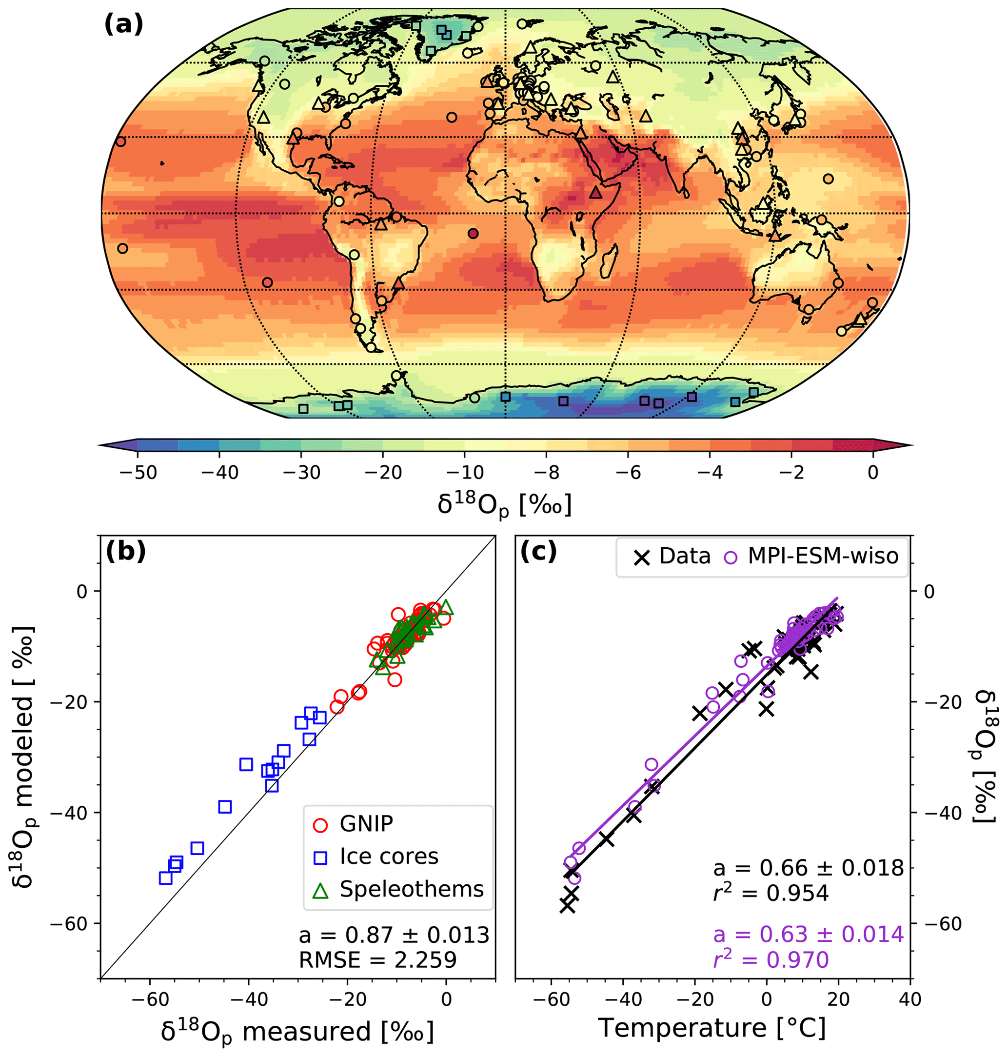
Figure 1(a) Global distribution of simulated (background pattern) and observed (colored markers; see text for details) annual mean δ18Op values in precipitation under PI conditions. The data consist of 70 GNIP stations (circles), 15 ice core records (squares; Table 1) and 33 speleothem records (triangles). (b) Modeled vs. observed annual mean δ18Op at the different GNIP, speleothem and ice core sites. (c) Observed (black crosses) and modeled (purple circles) spatial δ18Op–T relationship for the sites where the observed annual mean temperatures are below C. The linear fits for the observed and modeled values are drawn as black and red lines, respectively. For both (b) and (c), the gradients of the linear regression fits are given in the legends.
3.1.2 Water isotopes in ocean surface waters
Figure 2a shows the global distribution of modeled annual mean δ18Ooce in ocean surface water (mean between 0 and 10 m of depth) and the comparison with the observations from the GISS database (colored dots). As expected from the data, we observe higher modeled δ18Ooce values in the low-latitude to midlatitude oceanic areas, which range between −0.2 ‰ in the Malaysian area and 1.1 ‰ in the Bermuda area. The higher values in the Atlantic Ocean can be explained by a net freshwater export of Atlantic Ocean water, which is transported westwards to the Pacific (Broecker et al., 1990; Lohmann, 2003; Zaucker and Broecker, 1992). Other high δ18Ooce values can be found in more localized areas like the Mediterranean Sea, the Red Sea, the Aden Gulf and the Persian Gulf, with δ18Ooce values reaching +3.9 ‰ in the latter. The regional net freshwater export again explains these increases in δ18Ooce values. Contrary to Werner et al. (2016), who observed high δ18Ooce values in the Black Sea, we obtain low δ18Ooce values between −1 and −2.7 ‰ in this small-scale area, which is in better agreement with the observations. This opposite result is due to the land–sea mask of higher resolution applied in our model (T63GR15 against T31GR30 used in Werner et al., 2016) that results in a narrower connection between the Black Sea and the Mediterranean Sea via the Aegean Sea. At high latitudes, the δ18Ooce values are lower than the average. In the Southern Ocean, the modeled δ18Ooce values are between −0.4 and −1 ‰, in agreement with the observations. The most 18O-depleted ocean surface waters are in the Arctic Ocean, where the δ18Ooce values decrease down to −13 ‰. These very low δ18Ooce values are mainly caused by highly 18O-poor Arctic river discharges combined with a strong stratification of the simulated Arctic Ocean water masses (not shown).
In a similar way as for the atmospheric part, we compare our simulated δ18Ooce values with the isotopic observations between 0 and 10 m of depth (GISS database; see Sect. 2.3) for a more quantitative evaluation of our model results (Fig. 2b). For the Atlantic Ocean (blue circles), the Pacific Ocean (red circles), the Indian Ocean (green circles) and the Southern Ocean (brown circles), the model–data comparison does not show any systematic deviations between the modeled δ18Ooce values and the GISS data, characterized by RMSE values lower than 1 ‰ (Atlantic: r2=0.83, RMSE =0.98 ‰; Pacific: r2=0.67, RMSE =0.68 ‰; Indian: r2=0.48, RMSE =0.44 ‰ and Southern: r2=0.68, RMSE =0.32 ‰). As already reported in Werner et al. (2016), the deviations from the observations are due to the overestimation of δ18Ooce values near river estuaries around the Amazon and the Sea of Okhotsk. For the Arctic Ocean, our simulated δ18Ooce values are in better agreement with the observations (r2=0.57, RMSE =1.61 ‰) compared to the results from Werner et al. (2016) (r2=0.33, RMSE =2.25 ‰). However, our simulated δ values are still lower than the observations for many data entries. Because of the strong stratification of the simulated Arctic Ocean water masses, the highly 18O-depleted water inflows from Arctic rivers remain in the upper layers of the Arctic Ocean without being well mixed with deeper waters.
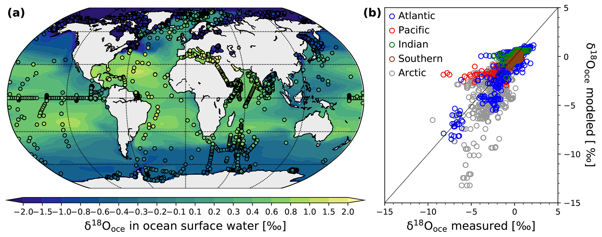
Figure 2(a) Comparison of the global distribution of simulated (background pattern) annual mean δ18Ooce values in ocean surface water (mean over the first 10 m of depth) under PI conditions with observed δ18Ooce values of the GISS database (colored dots). (b) Scatter plot of observed vs. modeled δ18Ooce values for the Atlantic (blue circles), Pacific (red circles), Indian (green circles), Southern (brown circles) and Arctic Ocean (grey circles). The month of sampling has been considered for this scatter plot.
In Fig. 3, we analyze the relationship between δ18Ooce in ocean surface water and salinity for the Atlantic (Fig. 3a), Pacific (Fig. 3b), Indian (Fig. 3c), Southern (Fig. 3d) and Arctic Ocean (Fig. 3e). MPI-ESM-wiso is in fairly good agreement with the observations in terms of absolute values and δ18Ooce–salinity gradients, the latter varying between 0.27 and 0.56 ‰ psu−1. The best agreements with the observations are in the Indian and the Pacific Ocean, even if the model is not able to reach the lowest δ18Ooce and salinity values around the Sea of Okhotsk and the Bering Sea. Except for the Pacific Ocean, the relationship between δ18Ooce and salinity in the different basins, expressed by the correlation coefficients r2, is stronger in the model (0.87, 0.90, 0.86, 0.67 and 0.87 for the Atlantic, Pacific, Indian, Southern and Arctic Ocean, respectively) than in the observations (0.56, 0.93, 0.70, 0.63 and 0.53, respectively). The main disagreement in the deduced δ18Ooce–salinity gradient is in the Atlantic Ocean, with a steeper gradient in MPI-ESM-wiso than in the GISS data. The latter is due to the underestimation by the model of the δ18Ooce values in the northwest Atlantic along the Canadian coast (Fig. 2). 18O-depleted water inflows from Canadian rivers and the strong ocean dynamics of this area with important interconnected currents, probably not well constrained by MPI-ESM-wiso, can explain the model–data mismatch. In the Arctic and Southern Ocean, even if the modeled δ18Ooce–salinity gradient is similar to the observed one, the model underestimates both the δ18Ooce and salinity values, probably because of the major roles played by river discharges and changes in sea ice in these areas.
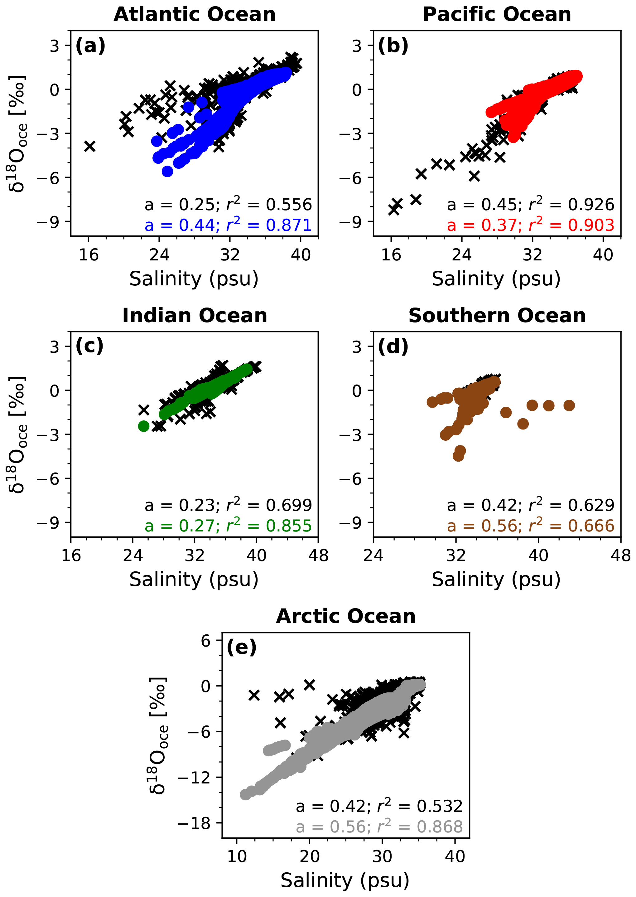
Figure 3Scatter plots of δ18O in ocean surface water vs. surface salinity for the (a) Atlantic, (b) Pacific, (c) Indian, (d) Southern and (e) Arctic Ocean under PI conditions. The black crosses correspond to the data from the GISS database and the colored dots to the modeled values. The gradients and the correlation coefficients of the linear regression fits are given in the legends.
3.1.3 Deuterium excess
The modeling of the deuterium-excess signal is challenging for GCMs. For the North Atlantic and Arctic Ocean region, the spatial structure of the marine boundary layer water vapor isotopic composition, which greatly influences the d-excess signal in precipitation, seems to be poorly simulated by the models (Steen-Larsen et al., 2017). Model deficits might be linked to sublimation and moisture source processes over sea-ice-covered areas (Bonne et al., 2019; Klein and Welker, 2016). Moreover, in higher latitudes, the representation of d-excess is very sensitive to supersaturation in polar clouds, which is a poorly constrained empirical parameter (Jouzel and Merlivat, 1984; Risi et al., 2013). A comparison of our simulated d-excess signals with available data thus represents a good evaluation test for our model. Figure 4 shows the simulated deuterium excess in precipitation (d-excessp) and ocean surface water (d-excessoce). The modeled values of d-excessp (Fig. 4a) range between 0 ‰ and 20 ‰. The highest values are in the northern part of the Sahara and in a 25–45∘ N band going from Saudi Arabia to the Himalaya. The lowest values are found in dry regions like the southern Sahara between the latitudes 25 and 10∘ N, Oman and Rajasthan (India), and over the Southern Ocean (between 2 and 6 ‰), which is an area with large net freshwater input (P−E). For the Antarctic continent, the contrast between the low values of d-excessp in the west and high values in the east is well captured by the model, in agreement with the observations. The quantitative model–data comparison (Fig. 4b) shows that the modeled d-excessp values are in fairly good agreement with the observations. However, MPI-ESM-wiso tends to underestimate the d-excessp values, especially where the observations are higher than 8 ‰.
The modeled d-excessoce values (Fig. 4c) range between −8 ‰ (Persian Gulf) and +7 ‰ (Baltic Sea). We can distinguish between the middle to low latitudinal region of the Atlantic Ocean with lower d-excessoce values (between −0.2 and −0.8 ‰), the Arctic Ocean where modeled d-excessoce values vary from 0 ‰ in the north of the Atlantic Ocean to +7 ‰ along the northern coast of Siberia, and the remaining ocean surface waters with smoother variations in their d-excessoce values (from −0.2 to 0.6 ‰). The negative d-excessoce signal in the middle to low latitudinal Atlantic Ocean is due to the presence of a net freshwater export. As the exported water masses and the evaporation have a positive deuterium-excess value, the d-excessoce in the remaining water becomes more negative due to the hydrological balance. This is the opposite for areas with positive d-excessoce values, like in the Baltic Sea and the Arctic Ocean, where there is a surplus of precipitation (positive P−E) with positive deuterium-excess values. The quantitative comparison with the GISS database (Fig. 4d) shows that MPI-ESM-wiso globally overestimates the deuterium-excess values in ocean surface water. The model is especially not able to reach the very low values observed in the Mediterranean Sea and overestimates the d-excessoce values in the Baltic Sea. Potential model–data mismatches can be due to different vertical layer thicknesses, which influence the surface kinetic fractionation. The horizontal model resolution, which is too coarse, can also affect the model–data comparison on a global scale, especially where strong small-scale variations in observed d-excessoce are found.
MPI-ESM-wiso overestimates the deuterium excess in the ocean surface and underestimates the deuterium excess in precipitation, especially for the highest observed values. However, the modeled linear relationship between the deuterium excess in water vapor above the ocean surface (d-excessvap) and the near-surface relative humidity (RH, expressed between 0 and 1) is , in very good agreement with the equation given by Pfahl and Sodemann (2014). One possible explanation for the positive and negative biases of modeled d-excess concentrations in the ocean surface water and precipitation, respectively, could be the description of fractionation processes during the evaporation of ocean surface water taken from Merlivat and Jouzel (1979), which would distribute too much d-excess in ocean surface water and not enough in the water vapor (and so in the precipitation). This agrees with the studies from Steen-Larsen et al. (2014a, b, 2015, 2017) and Bonne et al. (2019), which show biases in the simulated deuterium-excess signal in water vapor in Greenland, the North Atlantic and the Arctic Ocean in several GCMs compared to in situ measurements of surface water vapor isotopes.
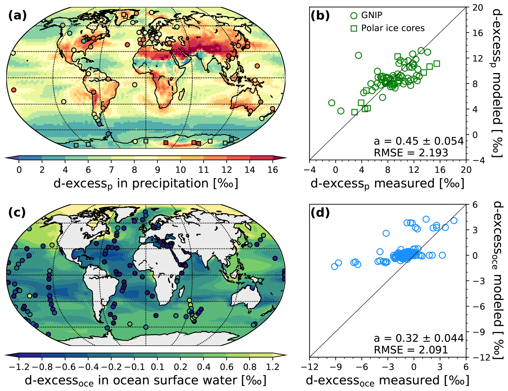
Figure 4Global distribution of simulated and observed annual mean d-excess values in precipitation (a) and ocean surface waters (c). Scatter plots of modeled vs. observed annual mean deuterium-excess values in precipitation (b) and ocean surface waters (d) are shown. The gradients and RMSE of the linear regression fits are given in the legend.
3.2 Mid-Holocene simulation
3.2.1 Changes in near-surface air temperature and precipitation
Before analyzing the 6k isotopic anomalies, we check that our modeled 6k−PI anomalies in standard climate variables, like the 2 m temperature and the precipitation rate, are consistent with previous studies. For that, we show in Fig. 5 the simulated annual mean boreal winter (DJF) and summer (JJA) changes in the 2 m temperature and precipitation rate between the 6k and PI climates. Because of the different values in orbital parameters and greenhouse gases, the mid-Holocene is characterized by a slightly colder mean global climate compared to the modeled PI (−0.42 ∘C). The simulated anomalies in annual mean temperature are rather small, with 6k−PI changes of less than 1 ∘C (Fig. 5a) in most regions. The exception is the Saharan area where a cooling in the range of −1 to −4 ∘C can be observed due to the enhanced African monsoon. We also observe a slight increase in annual mean temperature over the western Arctic area, northern Siberia and eastern Europe. As a first result, we conclude that the 6k−PI anomalies in annual mean temperature from MPI-ESM-wiso are globally consistent with the PMIP2 and CMIP5/PMIP3 model results (Harrison et al., 2014). The annual mean change in precipitation amount is very small (less than 1 mm yr−1), in agreement with the previous PMIP2 and CMIP5/PMIP3 model results (Harrison et al., 2014). The African (20∘ W–30∘ E, 10–20∘ N region) and Indian (70–100∘ E, 20–40∘ N region) monsoons are enhanced during mid-Holocene by +1.06 and +0.37 mm d−1, respectively (Fig. 5d), consistent with the PMIP3 results (https://pmip3.lsce.ipsl.fr, last access: 20 September 2019). The changes in orbital forcing lead to a northward expansion of the African monsoon. This is also in agreement with previous coupled model results (Braconnot et al., 2007; Harrison et al., 2014), even if this monsoon extension is still not large enough compared to the observations (Perez-Sanz et al., 2014).
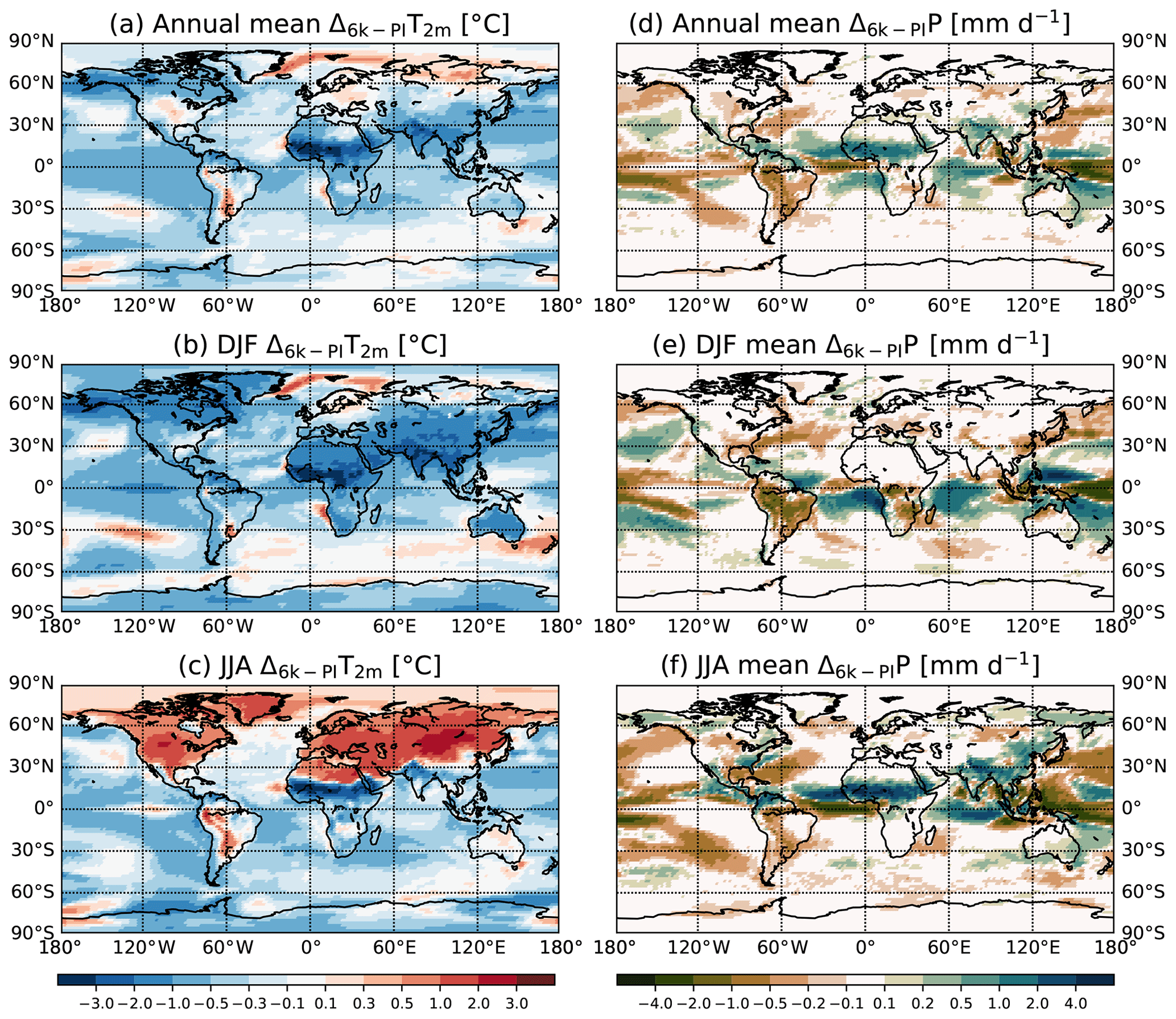
Figure 5Simulated annual, boreal winter (DJF) and boreal summer (JJA) changes in 2 m temperature (a, b, c) and precipitation (d, e, f) between 6k and PI.
One of the characteristics of the 6k climate is the enhanced seasonal contrast in the Northern Hemisphere due to changes in the insolation, giving rise to warmer Northern Hemisphere summers (Fig. 5c). There is a strong land–ocean contrast, with the main positive temperature anomalies on land. They range between +0.5 and +3 ∘C, the highest values being over North America and Mongolia, while the 6k−PI summer temperature anomalies in middle and high latitudes over the ocean and the Arctic are lower than 0.5 ∘C, except near the Greenland coasts. In lower Northern Hemisphere latitudes, the summer surface temperature anomalies over the ocean are generally lower (between 0 and −1 ∘C). In the Southern Hemisphere, positive mean JJA temperature anomalies (i.e., austral winter) can be observed over South America, Australia and coastal West Antarctica. The mean 6k JJA temperature anomalies over the ocean are globally lower, except for some locations in the Southern Ocean near the Antarctic coast. All these results are consistent with the previous PMIP simulations (Braconnot et al., 2007; Harrison et al., 2014). The colder 6k boreal summer in the region from West Africa to India is the consequence of increased precipitation linked to the monsoon changes (Fig. 5f) over this area (Braconnot et al., 2007). The positive anomalies in precipitation over Africa and India are the strongest during the boreal summer, with mean values of +2.42 and +1.00 mm d−1, respectively. We also find a dipole in the response of the monsoons over the Pacific–Indian area, with enhanced rainfall in the Equator sector of the Indian Ocean and reduced rainfall over the Indonesian region. For the mean DJF temperatures (Fig. 5b), we find negative anomalies over the Antarctic continent and positive anomalies over the surrounding Southern Ocean (between 0 and 0.5 ∘C). Over the rest of the globe, the 6k−PI anomalies in mean DJF surface temperatures are generally negative.
3.2.2 6k changes in δ18O signals
Even if the changes in temperature and precipitation amount are modest compared to periods like the LGM, they leave imprints on δ18Op in precipitation values (Fig. 6a). MPI-ESM-wiso simulates a precipitation-weighted mean global decrease in δ18Op by −0.16 ‰, which is in good agreement with the model results from LeGrande and Schmidt (2009). Positive simulated 6k−PI δ18Op changes, ranging from +0.3 to +1 ‰, are found over the Arctic area including Greenland, Alaska and the northern part of Siberia. They are likely associated with higher summer temperatures and reductions in Arctic sea ice during 6k (LeGrande and Schmidt, 2009). For the distribution of δ18Op anomalies over Antarctica, three areas can be distinguished: one region from the 180th meridian to 90∘ W with anomalies slightly negative or close to zero, another area from 90∘ W to 100∘ E with positive anomalies of δ18Op, and the remaining region between 100 and 180∘ E with negative isotopic anomalies. Except for Australia, the Indonesian area and some coastal regions in the American continent, negative 6k−PI changes occur in general over the remaining land surfaces. The strongest negative anomalies (−5.43 ‰) are located over the southern Sahara where a strong decrease in surface temperature and amplified African monsoon are simulated by MPI-ESM-wiso. Strong negative changes in δ18Op also occur over the Tibetan Plateau, with values ranging from −0.5 to −3.5 ‰. This is probably due to the lower simulated values of annual mean temperature in this area during the 6k period combined with an enhanced precipitation rate, especially in summer (Fig. 5). Finally, MPI-ESM-wiso simulates positive 6k−PI anomalies of δ18Op between +0.2 and +1 ‰ in the western Pacific Ocean and over the Indonesian area linked to lower rainfall during mid-Holocene.
Next, we compare our simulated 6k−PI δ18Op anomalies with isotopic observations from the ice cores and speleothem records described in Sect. 2.3 (Fig. 6b). In general, our modeled isotopic anomalies are in fair agreement with the data (r2=0.38 and RMSE =0.79 ‰). The modeled positive δ18Op anomalies over most parts of Greenland are confirmed by the polar ice core measurements and the negative anomalies over the southern Greenland coast. The largest deviation is found for the coastal Renland ice core () for which MPI-ESM-wiso simulates a δ18Op anomaly of +0.25 ‰, which is too low. The modeled positive–negative contrast in the Δ6k−PIδ18Op distribution between the central and eastern parts of Antarctica is also found in the data (EDC, Vostok and Talos ice cores in the east; Dome Fuji and EDML in the central area). However, there is a disagreement in the west of the continent, with modeled δ18Op anomalies close to zero, while the observations are clearly positive (WDC ice core) or negative (Byrd and Siple Dome ice cores). In the most eastern region of Antarctica (160∘ E), near the Ross Sea, MPI-ESM-wiso is not able to catch the positive 6k−PI δ18Op anomaly at the Taylor Dome site. Concerning the δ18O anomalies from calcite in speleothems, all our simulated 6k−PI isotopic changes are of the same sign as the speleothem data if we include an uncertainty of ±0.5 ‰, as in Comas-Bru et al. (2019). The model reproduces the observed negative and positive 6k−PI changes in δ18Oc well over the Tibetan Plateau and the coastal areas of the South American continent, respectively. Disagreements with the speleothem data are found in the US and in Europe where observed positive anomalies are not captured by MPI-ESM-wiso. The largest deviations are found for two speleothems located in Ethiopia ( and ) and in the Great Basin of western North America ( and ). These discrepancies likely reflect an insufficient amplification of the precipitation rate (or its wrong location) over eastern Africa and an increase in temperature that is too weak over northeast America during the mid-Holocene period. More generally, the amplitude of the modeled δ18O changes at speleothem sites is underestimated by MPI-ESM-wiso. This is likely related to the underestimation by the model of the 6k changes in climate variables like the temperature and precipitation rate, as already noticed in previous model studies (Harrison et al., 2014).
Concerning the changes in d-excessp in precipitation, we find negative anomalies over Antarctica and Greenland. The modeled d-excessp value at the EDC site is of opposite sign compared to the measured value ( and ), while the Greenland values are consistent with the observations (GRIP: and ; NGRIP: and ).
Figure 7 shows our modeled annual mean changes in δ18Ooce in ocean surface water between 6k and PI. The simulated annual mean δ18Ooce change between 6k and PI is very small (−0.01 ‰), in agreement with previous model results (LeGrande and Schmidt, 2009). The model simulates an increase in δ18Ooce in the Arctic Ocean ranging from 0.1 to 0.7 ‰, except around the 180th meridian, which is related to Arctic sea ice reductions and warmer summers in 6k relative to PI. Higher δ18Op values in precipitation are observed, too. Enhanced runoff with lower δ18O values (not shown) is associated with negative 6k−PI anomalies in δ18Ooce along the coasts of central America and southwestern Africa, the Red Sea, the Persian Gulf, and the Bay of Bengal. As for the changes in δ18Op, MPI-ESM-wiso simulates a dipole of higher–lower δ18Ooce values compared to the PI state in the western Pacific Ocean (from +0.05 ‰ to +0.5 ‰) and the Bay of Bengal (from −0.05 ‰ to −1 ‰), respectively. Positive δ18Ooce changes are also found in the subtropical latitudes of the eastern Pacific Ocean. The increase in δ18Ooce values during 6k relative to PI is due to the lower annual mean precipitation rates over these areas and vice versa. Slight positive δ18Ooce anomalies are also simulated along the western Antarctic coast related to the higher 6k summer temperatures over the Southern Ocean.
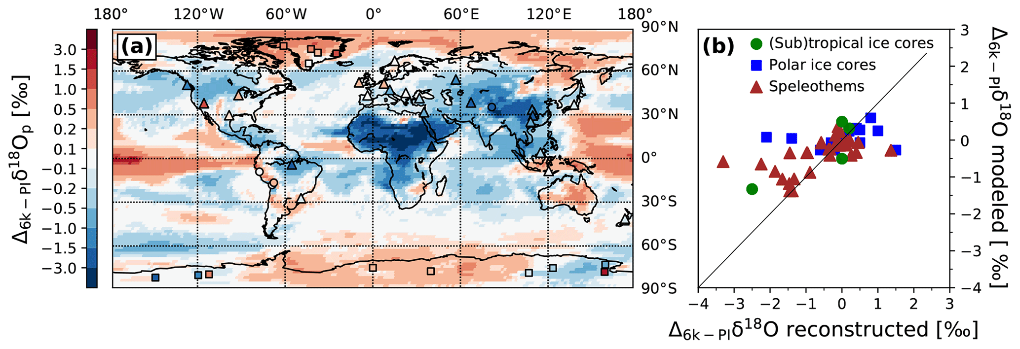
Figure 6(a) Simulated global pattern of annual mean δ18Op changes in precipitation between the mid-Holocene and PI climate as well as a comparison with reconstructed δ18O changes in polar (squares) and (sub)tropical (dots) ice cores and in calcite speleothems (triangles). (b) Reconstructed δ18O changes from ice cores and speleothems vs. simulated 6k–PI δ18O anomalies at the same location. The observed δ18O anomalies in polar and (sub)tropical ice core records (blue squares and green dots, respectively) are compared to the simulated 6k–PI δ18Op changes in precipitation. The observed Δ6k−PIδ18O in speleothems (brown triangles) are compared to simulated δ18Oc changes in calcite (see text).
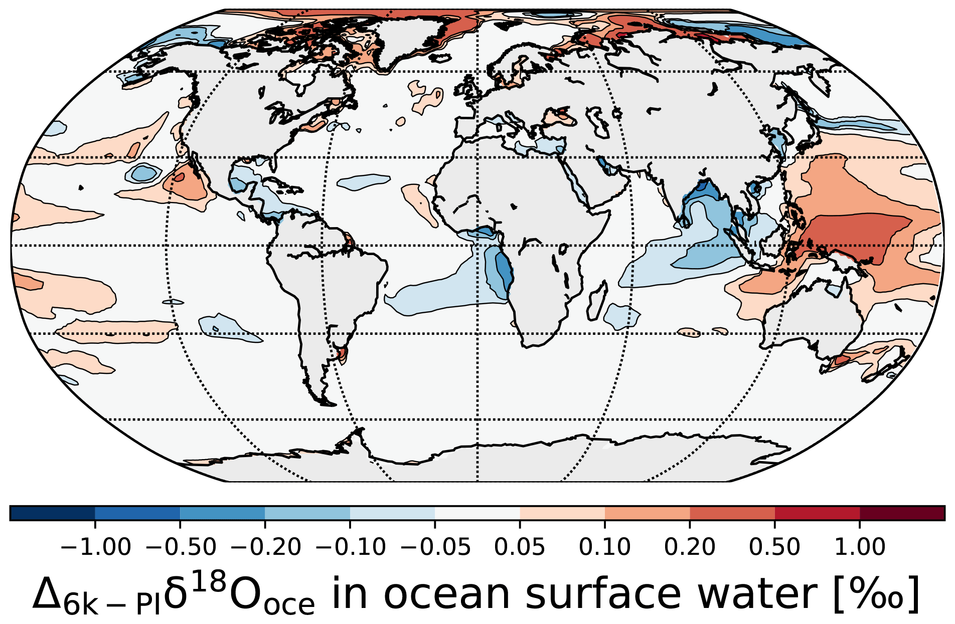
Figure 7Modeled annual mean δ18Ooce changes in ocean surface water between the mid-Holocene and PI climate.
The classical use of water isotopes to reconstruct past variations of climate implies that the modern spatial relationship between isotopes and climate variables, such as surface temperature, precipitation rate and salinity, can be taken as a surrogate for the temporal isotope–climate gradient at a given site. Such temporal relationships can be calculated from our model results. In Sect. 4.1, we first look at the interannual variability between water isotopes and 2 m temperature, precipitation rate and salinity under PI conditions. We limit the analysis to the interannual gradients from our PI simulation as they are qualitatively similar to the ones derived from our 6k simulation. The corresponding figures for the 6k period (Figs. S1 and S3) and their differences from PI results (Figs. S2 and S4) are in the Supplement. Then, we examine the long-term temporal 6k−PI δ18O gradients versus the different climate variables in Sect. 4.2.
4.1 Interannual relationships of water isotopes and climate variables for the PI climate
In the same way as previous studies (Schmidt et al., 2007; Risi et al., 2010b; Roche and Caley, 2013), we calculate for each grid box the interannual relationship (correlation coefficients and gradients) between monthly anomalies of δ18Op and temperature and precipitation rate over the 150 years of our PI simulation. These monthly anomalies are calculated by subtracting from each monthly mean value the multi-year mean value of the corresponding month; e.g., we subtracted the long-term January mean value from the January values. For the following, we consider only the grid boxes with a temporal correlation higher than 0.4 in absolute value (Risi et al., 2010b; Roche and Caley, 2013). By introducing such a correlation threshold, we remove any grid cell with a negative δ18Op–temperature gradient (for which precipitation rates are higher) and/or positive δ18Op–precipitation gradient (for which precipitation rates are too low) not physically plausible. The temporal correlations of δ18Op with temperature are positive (Fig. 8a) in the middle- to high-latitude grid boxes, i.e., over Antarctica, North America, Greenland, Europe and the northern part of Russia. At these locations, the interannual δ18Op–temperature gradients vary between 0.3 ‰ ∘C−1 and 0.9 ‰ ∘C−1, with the highest values over the poles (Fig. 8b). For Greenland, we find a mean PI interannual δ18Op–temperature gradient of 0.57 ‰ ∘C−1, averaged over all Greenland ice core locations (Table 1) where the correlation coefficient is higher than 0.4 in absolute value. This is less than our modeled PI spatial gradient of 0.71 ‰ ∘C−1 (calculated by considering the 25 grid cells centered on each drill location, excluding the ocean grid points), in agreement with previous modeling studies (Werner et al., 2000; Schmidt et al., 2007). For the ice core locations in East and West Antarctica, the averaged modern spatial gradients are 0.76 ‰ ∘C−1 and 0.88 ‰ ∘C−1, respectively, in agreement with the mean observed value of 0.8 ‰ ∘C−1 (Masson-Delmotte et al., 2008) and previous model results (Schmidt et al., 2007; Werner et al., 2018). A clear distinction can be made between east and west when looking at the PI interannual δ18Op–temperature gradients. For East Antarctica, we obtain a value of 0.66 ‰ ∘C−1, close to the modern spatial gradient over this area. On the contrary, the mean interannual gradient at West Antarctic ice core sites is 0.39 ‰ ∘C−1 only, which is more than 2 times smaller than the corresponding average spatial gradient. This result, which could be related to sea ice variations or the large-scale transport of moisture from the ocean, will be investigated in a further study by comparison with other models results.
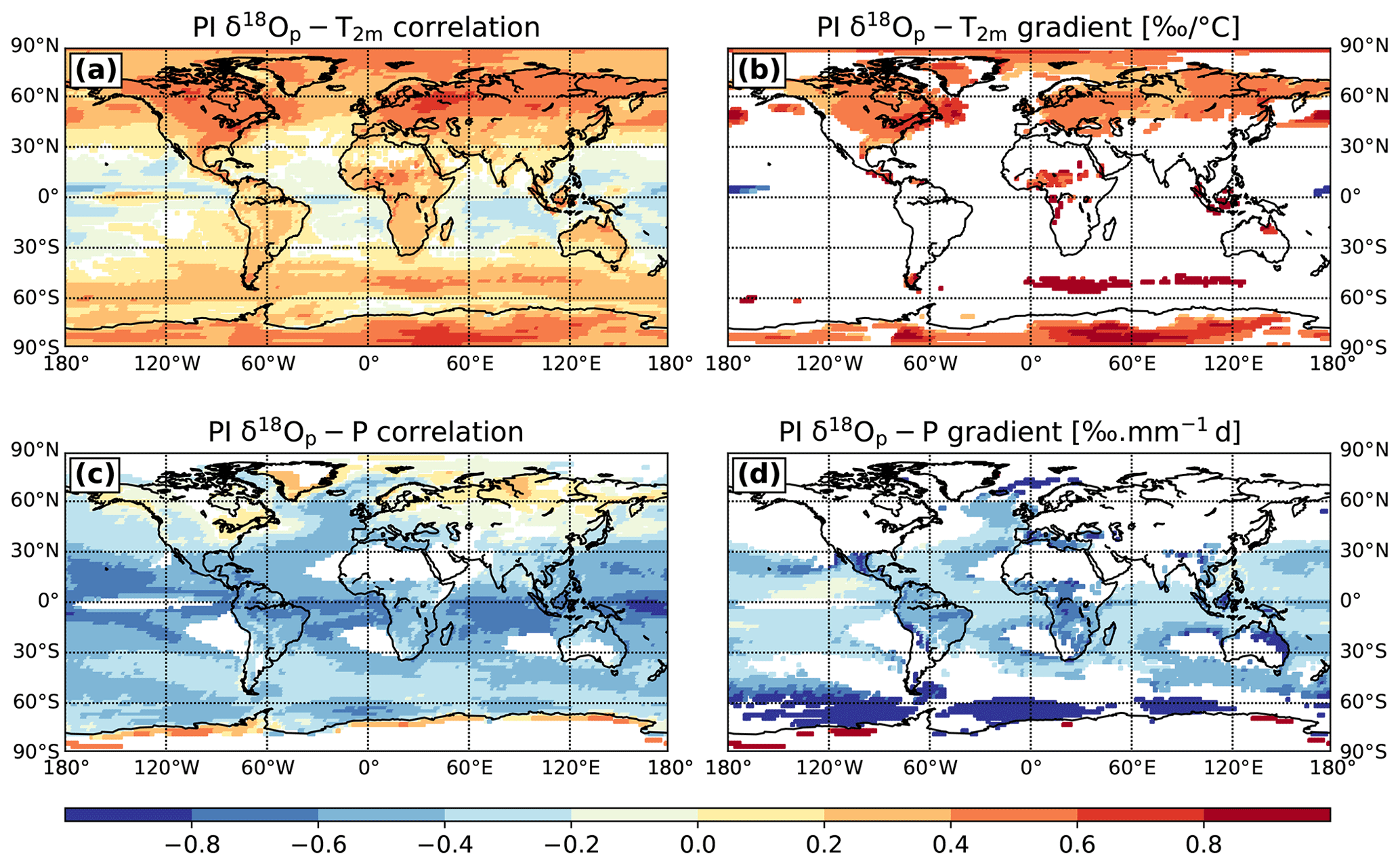
Figure 8Correlation coefficients (a, c) and gradients (b, d) of the interannual relationship between monthly anomalies of δ18Op in precipitation and temperature (a, b) as well as precipitation rate (c, d). All values shown are significant at the 95 % level. We restrict the analysis of the δ18Op–precipitation relationship to grid points with a mean precipitation rate higher than 250 mm yr−1. The gradient values are only shown for correlation coefficients higher than 0.4 in absolute value.
The correlation values between modeled monthly anomalies of δ18Op and precipitation rate are negative from the Equator to the midlatitudes (Fig. 8c). This area gathers the Indian, Pacific and Atlantic Ocean, Central and South America, and a part of the African continent. The interannual δ18Op–precipitation gradients vary from −0.2 ‰ mm−1 d to −0.8 ‰ mm−1 d (Fig. 8d). The lowest values are located over the Amazonian area, Central America and in the south of the Sahara, with temporal gradients steeper than −0.5 ‰ mm−1 d. For example, we find a mean value of −0.61 ‰ mm−1 d over the African monsoon area, consistent with previous model results (Schmidt et al., 2007; Risi et al., 2010b). We obtain an interannual δ18Op–precipitation mean gradient of −0.38 ‰ mm−1 d at cells in which the annual mean temperature is equal to or greater than +20 ∘C, consistent with the observed and modeled spatial PI gradients (−0.46 ‰ mm−1 d and −0.36 ‰ mm−1 d, respectively).
In a similar way to the atmospheric relationships, we assess the temporal gradients between monthly anomalies of δ18Ooce in ocean surface water and salinity under PI conditions. The modeled δ18Ooce PI interannual variations are strongly correlated with the salinity changes (Fig. 9a) almost everywhere, with a mean correlation coefficient r=0.82 (standard deviation σ=0.19). The lowest correlation values (r between 0.2 and 0.8) are located at the high latitudes near the Antarctic coasts and in the Arctic area due to the presence of sea ice, as well as in several (sub)tropical areas (west of the Sahara and 170∘ E–100∘ W, 10∘ N–30∘ S), probably because of the influence of precipitation amounts on the isotopic concentrations. The mean value of the PI temporal gradients is 0.33 ‰ psu−1 (Fig. 9b). Generally, gradients are steeper in the middle to high latitudes (between 0.3 ‰ psu−1 and 0.7 ‰ psu−1) and shallower in the tropics (between 0.1 ‰ psu−1 and 0.3 ‰ psu−1), in agreement with previous model results (Schmidt et al., 2007; LeGrande and Schmidt, 2011). In the western Pacific–Indian Ocean area, the gradients are slightly steeper than in the rest of the tropical ocean (more than 0.3 ‰ psu−1), possibly due to the region's central role in exporting water vapor to the extratropics (Schmidt et al., 2007). We obtain mean PI interannual δ18Ooce–salinity gradients of 0.30, 0.29, 0.29, 0.38 and 0.40 ‰ psu−1 for the Atlantic, Pacific, Indian, Southern and Arctic Ocean, respectively. Except for the Indian Ocean, the mean modeled spatial gradients (Fig. 3) are steeper than the interannual ones, in agreement with previous model results (Holloway et al., 2016).
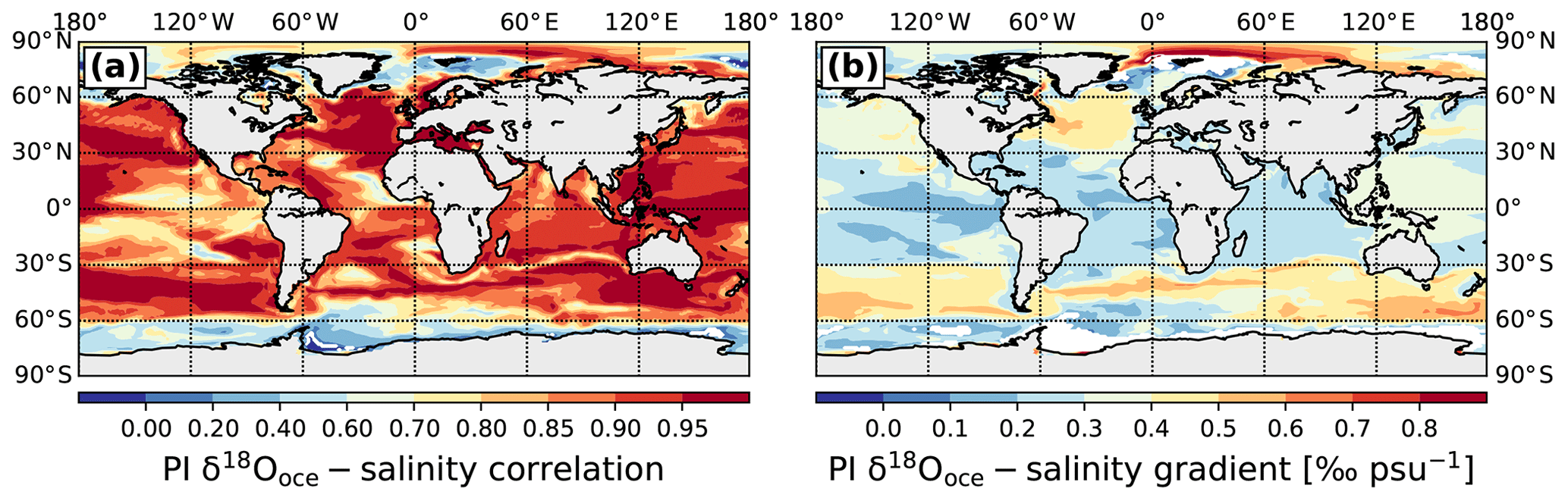
Figure 9Correlation coefficients (a) and gradients (b) of the interannual relationship between monthly anomalies of δ18Ooce in ocean surface water and salinity. All values shown are significant at the 95 % level. The gradient values are only shown for correlation coefficients higher than 0.4.
4.2 Temporal relationships of water isotopes and climate variables between 6k and PI
The global spatial relationship between climate variables and water isotopes does not change significantly between our simulated mean climate states of 6k and PI. For example, we find a mean spatial δ18Op–temperature regression gradient of 0.63 ± 0.014 ‰ ∘C−1 for the 6k simulation, similar to the PI one (Fig. 1c). The surface relationships between δ18Ooce and salinity in the different oceans for the PI (Fig. 3) and 6k periods are extremely similar, too. Now, we examine the calculated 6k−PI temporal relationship between different climate variables (temperature, precipitation and ocean salinity) and δ18O changes. If we take as an example the temporal relationship with temperature (T) changes, the temporal gradient m of each grid cell is calculated as . For the latter, we restrict our calculation to the grid boxes in which the simulated mean temperature is below +20∘C for both PI and 6k. Moreover, we select only the grid cells showing an absolute temperature 6k−PI difference of at least 0.5∘C. We present the results in a histogram (Fig. 10a) and global maps (Fig. 10b, c and d). By using the values of mean annual temperatures (MAT) and δ18Op, the calculated temporal 6k−PI gradient is below the spatial PI gradient (dotted line in Fig. 10a) in 79 % of the grid cells considered (red bars in Fig. 10a). Only 10.1 % of the selected grid cells (229 on 2273) have a temporal gradient between 0.5 ‰ ∘C−1 and 0.7 ‰ ∘C−1, close to the simulated PI spatial gradient. Upon examination of the corresponding map (Fig. 10b), it appears that the δ18Op–T temporal relationship can have negative (north of Canada, Alaska and the western coast of South America) or very high gradients (over China and north of India) at certain locations. For the first case, the small difference between the modeled 6k and PI annual mean temperatures (less than 1 ∘C; Fig. 5a) and a strong seasonality of precipitation can probably lead to meaningless δ18Op–T gradients (Gierz et al., 2017). For the second case, changes in the monsoon strength can explain the very high δ18Op–T gradients (more precipitation combined with lower temperatures). One can also notice that only very few grid cells over Greenland and Antarctica, where the correlation between the isotopic content in precipitation and the temperature is high, are in accordance with the selection criteria described above.
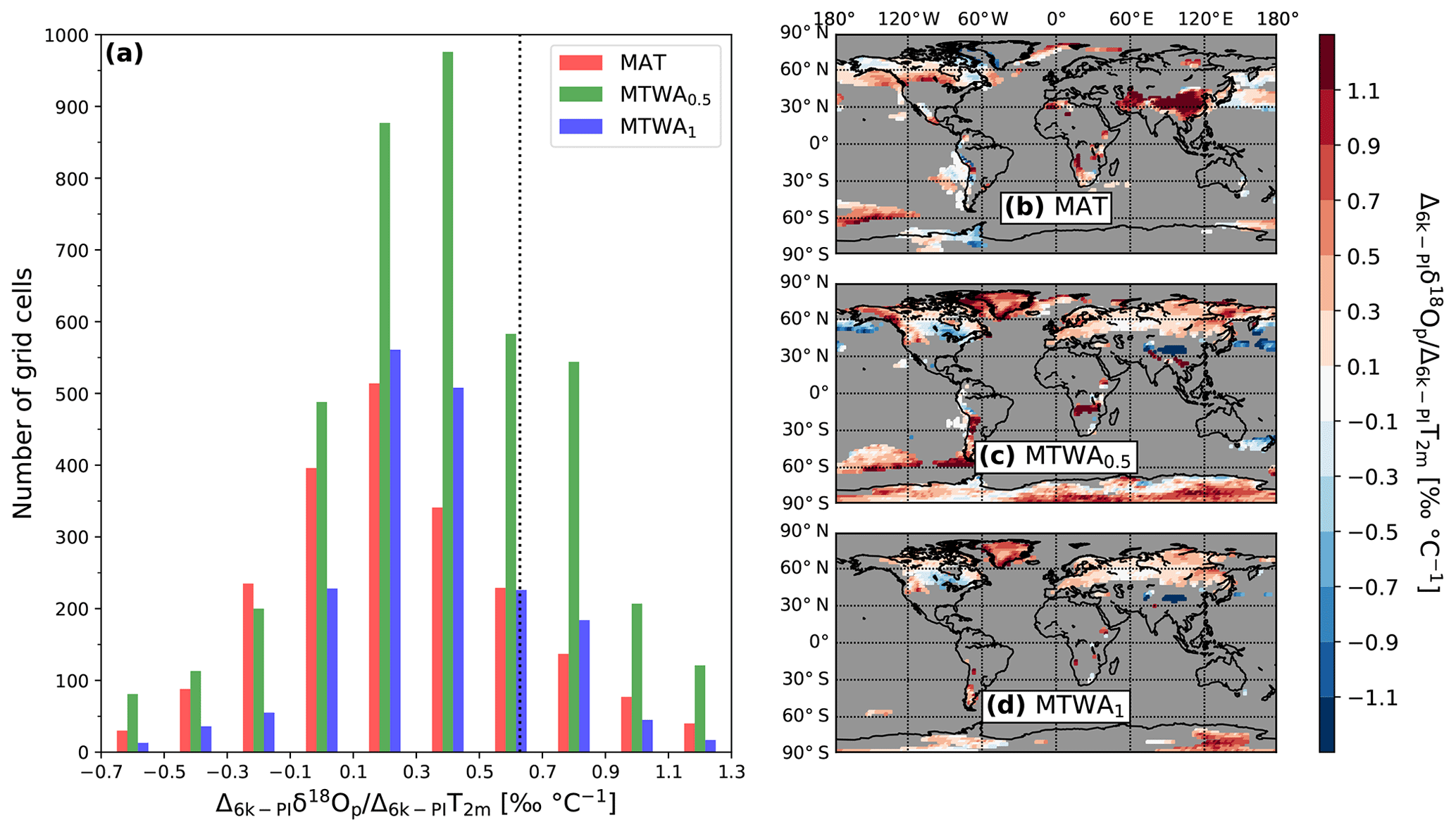
Figure 10(a) Histogram of the calculated temporal 6k–PI δ18Op–T gradients for all grid cells in which (i) simulated mean temperature for both PI and 6k is lower than 20 ∘C and (ii) absolute change in temperature between the 6k and PI control simulations is at least 0.5 ∘C (MAT, WTMA0.5) or 1 ∘C (WTMA1). The dotted line shows the simulated mean spatial PI δ18Op–T gradient of 0.63 ‰ ∘C−1. The gradients are calculated in three different ways: with the annual mean δ18Op and temperature values where C (MAT, red bars), with the mean δ18Op and temperature values of the warmest month where C (WTMA0.5, green bars), and with the mean δ18Op and temperature values of the warmest month where C (WTMA1, blue bars). Their spatial distribution is shown in (b), (c) and (d), respectively.
For numerical reasons, robust δ18Op–T gradients can only be calculated for non-negligible 6k−PI temperature anomalies. In a next step, we therefore analyze not the mean annual temperature values but the modeled mean values of the warmest month, i.e., the mean temperature values of July for the Northern Hemisphere and January for the Southern Hemisphere (MTWA: mean temperature of the warmest month). The frequency distribution of the temporal gradients using this new calculation corresponds to the green bars in Fig. 10a (MTWA0.5), and the global map is shown in Fig. 10c. From this map, we can see that δ18Op–T temporal gradients can be calculated for the grid boxes at middle to high latitudes. This is reflected by a higher proportion of 6k−PI temporal gradient values that are between 0.5 ‰ ∘C−1 and 0.7 ‰ ∘C−1 (13.1 % of the grid cells, i.e., 583 of 4438). The resulting mean 6k−PI temporal gradients around ice core locations in East Antarctica, West Antarctica and Greenland are 0.52, 0.52 and 1.36 ‰ ∘C−1, respectively. These temporal gradients calculated from our 6k and PI isotopic simulations are substantially different from the modeled surface gradients: higher for Greenland and lower for East and West Antarctica. Because a non-negligible portion of the analyzed grid cells still reveals a negative δ18Op–T temporal gradient, we increase the temperature cutoff from 0.5 to 1 ∘C (WTMA1). Despite this stronger restriction, the proportion of grid boxes having δ18Op–T gradient values between 0.5 ‰ ∘C−1 and 0.7 ‰ ∘C−1 remains almost the same (11.8 % of the grid cells, i.e., 226 of 1908). However, applying this temperature restriction removes many of the grid boxes with negative or very high gradients (blue bars in Fig. 10a), like in central Antarctica (Fig. 10d). The mean 6k−PI temporal gradients around Greenland and East Antarctic ice core locations are equal to 0.77 ‰ ∘C−1 and 0.82 ‰ ∘C−1, respectively. These values are very close to the modeled spatial PI gradients of 0.71 ‰ ∘C−1 and 0.77 ‰ ∘C−1. These results could mean that the spatial gradients are more of a surrogate for summer temperature variations between 6k and PI, especially over Greenland where the seasonality is enhanced in 6k compared to PI. This result has to be taken with caution, especially for the East Antarctic area where only the EDC site satisfies the required conditions for the gradient calculation. Under this new condition, it is also not possible to calculate a mean temporal δ18Op–T gradient for West Antarctic ice core locations.
The δ18Op values in polar region grid boxes might be biased by strong changes in the seasonality or intermittency of the precipitation rate (Sime et al., 2009). So, in the same way as Gierz et al. (2017), we replace the arithmetic annual mean temperatures by the precipitation-weighted annual mean temperatures in the calculation of the δ18Op–T gradients (Fig. 11). With this new calculation, we obtain mean 6k−PI temporal gradients of 0.58, 0.38 and 0.01 ‰ ∘C−1 for the grid cells around the Greenland, East Antarctic and West Antarctic ice core locations, respectively. This shows the effects of seasonality well on the δ18Op–T gradients over Greenland and, to a lesser extent, over East Antarctica. The great variability of the resulting mean temporal gradients for the West Antarctic ice core locations (e.g., mean values near zero, positive or not meeting the requirements for temperature difference) could indicate that temperature changes between the warm 6k and PI periods are not the main driver of the variations of δ18Op in this area. The contrast in the δ18Op–T gradient between West Antarctica, which is more sensitive to moisture inputs from coast regions, and East Antarctica, the stronger isolated plateau region, is also visible in the δ18Op anomalies between 6k and PI (Fig. 6a).
The δ18Op in precipitation over West Antarctica could be sensitive to a more important contribution of relatively 18O-rich evaporating water from the surrounding ocean near the coast during 6k linked to the increased divergence of sea ice and enhanced open-water areas around the coast (Noone and Simmonds, 2004). We also observe slight positive austral summer (DJF) sea surface temperature anomalies (between 0 and 0.5 ∘C) in the western Southern Ocean area, while the entire Antarctic continent is cooler (middle left map of Fig. 5), and an increase between 5 % and 20 % in the evaporation flux around the Antarctic coasts. This sea ice hypothesis can be checked by looking at the changes in the vertically integrated water vapor transport over Antarctica between PI and 6k climates (Fig. 12). We focus on the warmest season (DJF) and see that the western part of the continent is clearly exposed to water vapor input coming from regions near the Antarctic Peninsula, the Ross Sea and the Amundsen Sea. But no significant differences in the water vapor transport pattern can be observed between our PI and 6k climates. However, positive annual mean 6k−PI anomalies of δ18O in vertically integrated water vapor (between 0.1 ‰ and 0.4 ‰) are simulated by the model over the Southern Ocean, which cannot be simply explained by changes in temperature as the latter are not strong enough. Thus, insolation variations apparently lead to seasonality changes that alter the δ18Op in the precipitation signal independent of temperature changes over the polar regions during the mid-Holocene.

Figure 11Spatial distribution of the calculated temporal 6k–PI δ18Op–T gradients for all grid cells in which (i) simulated annual mean temperature for both PI and 6k is lower than 20∘C and (ii) absolute change in temperature between the 6k and PI control simulations is at least 0.5∘C. The gradients are calculated in the same way as in Fig. 10b but with the use of precipitation-weighted temperatures instead of arithmetic annual mean temperatures.
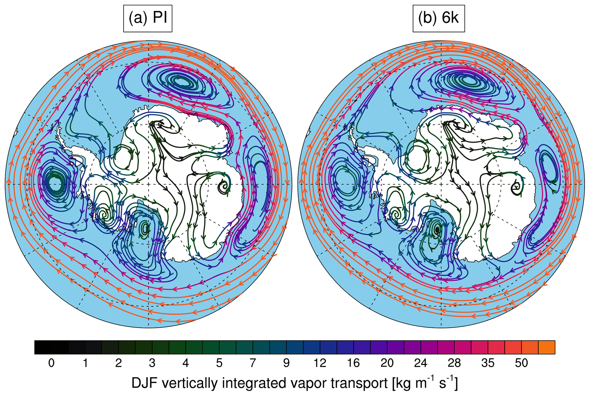
Figure 12Vertically integrated water vapor transport over Antarctica during austral summer for PI (a) and 6k (b).
According to our model results, the Indian and African monsoons are enhanced during the mid-Holocene compared to the preindustrial period (Sect. 3.2.1). As a consequence, the precipitation over these areas has lower δ18Op values, consistent with the amount effect (Fig. 6). The modeled mean 6k−PI temporal δ18Op–precipitation gradient over the African monsoon for the summer months (JJA) is equal to −1.52 ‰ mm−1 d, which is higher in absolute value than the interannual gradient (Sect. 4.1). If we consider annual averages instead of JJA values, the mean δ18Op–precipitation gradient is even steeper, with a value of −4.15 ‰ mm−1 d, because of the larger impact on the average anomaly in precipitation than on the 6k–PI changes in annual mean precipitation-weighted δ18Op. This result is in agreement with the finding from Risi et al. (2010b). Our results indicate that the amount effect may strongly depend on the considered timescale and that the use of a calibration based on a present-day interannual scale can be misleading for reconstructing past precipitation rates (Schmidt et al., 2007; Risi et al., 2010b). This is also indicated by the very high regional variability of the 6k−PI δ18Op–precipitation gradients over the African monsoon area (standard deviation of 1.90 ‰ mm−1 d for the mean JJA δ18Op–precipitation gradient).
Figure 13 presents a distribution map of the temporal 6k−PI δ18Ooce–salinity gradients for every oceanic surface grid cell. The calculation is restricted to the grid cells in which the 6k−PI absolute change in salinity is equal to or higher than a threshold value of 0.02 psu. We find a global mean gradient of 0.36 ‰ psu−1, close to the modeled interannual mean gradient. However, the mean 6k−PI δ18Ooce–salinity gradients in the different oceans can be significantly different from the mean modeled interannual gradients in these same oceans. For the Atlantic Ocean, the averaged 6k−PI δ18Ooce–salinity gradient is 0.22 ‰ psu−1, which is shallower than the modeled interannual gradient (Fig. 9b), itself shallower than the spatial PI gradient (Fig. 3a). However, strong 6k−PI gradients are simulated in the North Atlantic (between 0.6 and 1.25 ‰ psu−1), much higher than the PI interannual ones (0.4–0.6 ‰ psu−1). The mean gradient in the Pacific Ocean is similar to the interannual gradient, but higher values are modeled in the 10–30∘ N area linked to the 6k−PI changes in the precipitation rate. The mean temporal 6k−PI δ18Ooce–salinity gradient in the Indian Ocean (0.37 ‰ psu−1) is higher than the corresponding mean PI interannual and spatial gradients. We especially notice steep gradient values near the Bay of Bengal (coincident with lower δ18Ooce values during the 6k period) due to the enhanced runoff during the mid-Holocene period (Sect. 3.2.2). This pattern, even if it is not as well expressed, is also visible in the Arabian Sea. The average of the 6k−PI gradients in the Southern Ocean is similar to the interannual one (0.37 ‰ psu−1), while the mean gradient in the Arctic Ocean is similar to the δ18Ooce–salinity spatial relationship (0.56 ‰ psu−1). However, there is a strong spatial variability in the calculated gradients because of the changes in sea ice coverage and/or weak 6k−PI differences in salinity.
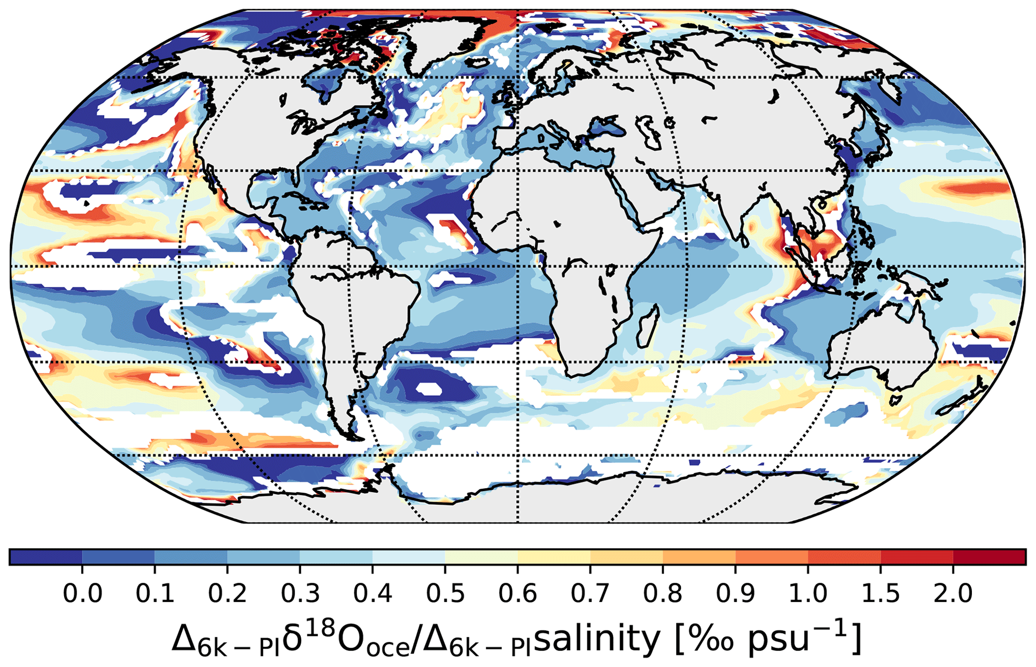
Figure 13Spatial distribution of calculated temporal 6k–PI δ18Ooce–salinity gradients for oceanic grid cells in which the 6k–PI absolute change in salinity is at least 0.02 psu.
We conclude that the reconstruction of past salinity through the isotopic content in sea surface waters can be complicated for regions with strong ocean dynamics (North Atlantic Ocean), variations in sea ice regimes (Arctic and Southern Ocean) or significant changes in the freshwater budget (Bay of Bengal), giving an extremely variable relationship between δ18Ooce and salinity over small spatial scales. This reconstruction task is even more difficult because of the small 6k−PI changes in salinity that can lead to large uncertainties in the calculated δ18Ooce–salinity gradients.
In this study, we present the first simulations of the fully coupled model MPI-ESM, enhanced with water isotope diagnostics. The water isotopes have been implemented in all the components of the model (atmosphere, dynamic vegetation, hydrological discharge, ocean–sea ice), and the related isotope masses of , and HD16O are fully exchanged between the atmosphere and the ocean. The model has been run successfully for 2500 model years under PI and 6k conditions. The PI spatial distribution of modeled isotopes in precipitation and ocean surface water has been evaluated against present-day observations from the GNIP and GISS databases, ice cores, and speleothems. For precipitation, we find a good to very good agreement of δ18Op values with the observational data. The modeling of δ18Op over Antarctica is especially improved compared to the previous model release ECHAM5/MPIOM (Werner et al., 2016) through the better ability of our model to reach the lowest temperatures due to overall model enhancements and a higher spatial resolution. Our modeled δ18Ooce in ocean surface water is in fairly good agreement with the isotopic observations from the GISS database. For the Atlantic, Pacific and Indian Ocean, the main model–data deviations are found near river estuaries, where the coarse resolution of MPIOM hampers a realistic simulation of water mass mixing near the coastal regions. In the Arctic Ocean, improvements in the δ18Ooce model–data agreement are found compared to Werner et al. (2016), but many model values are still too low compared to the observations. This could be related to the influence of sea ice in the area and/or to the inadequate mixing of highly 18O-depleted water from Arctic rivers into the ocean. The PI simulated values of the 2nd-order parameter d-excess are in fairly good agreement with the isotopic observations in precipitation and ocean surface water. MPI-ESM-wiso underestimates the deuterium-excess values in precipitation and, at the same time, overestimates the deuterium-excess values in ocean surface water. This pattern, already observed by Werner et al. (2016) with ECHAM5/MPIOM, suggests that the approach by Merlivat and Jouzel (1979) used in our model setup to describe the fractionation processes during evaporation over the ocean should perhaps be revised in the future. Finally, the simulated modern spatial relationships between isotopes and climate variables (2 m temperature, precipitation rate and salinity) are in good agreement with the observed ones.
The modeled changes in temperature and precipitation rate during the mid-Holocene compared to the preindustrial period are consistent with previous PMIP results, with a warmer Northern Hemisphere summer and enhanced African and Indian monsoons. One great advantage of enabling MPI-ESM to model water stable isotopes is the possibility to directly compare available isotopic measurements with our climate simulations. We find a fair agreement between our modeled 6k isotopic anomalies and the observations from ice cores and speleothems. MPI-ESM-wiso simulates higher δ18Op values over Greenland linked to higher mid-Holocene summer temperatures and changes in sea ice. Over Antarctica, δ18Op anomalies reveal three different regions of change: no isotope changes over the west (180–90∘ W), positive δ18Op anomalies over the center (90∘ W–100∘ E) and negative anomalies over the most eastern part of the continent (100–180∘ E). Over the East Antarctic plateau, the negative anomalies are consistent with the ice core measurements and are likely related to variations in local temperature. The modeled positive 6k−PI changes in δ18Op over the 90∘ W–100∘ E Antarctic area, more influenced by evaporating waters from the Southern Ocean, are in agreement with the observations, too. The absence of δ18Op anomalies, according to MPI-ESM-wiso, in the western part of the Antarctic continent, disagrees with the available observations. In the tropics, δ18Op and δ18Ooce variations are linked to changes in the precipitation rate (amount effect), i.e., enhanced African and Indian monsoons with lower δ18O values and a lower precipitation rate with higher δ18O values over the tropical western Pacific Ocean and the Indonesian area.
In numerous previous paleoclimate studies, one of the main assumptions for using water isotopes to study past climate variations is that the modern spatial isotope–climate variable relationships can be used as a surrogate for the temporal gradients at any specific site. In this study, we focused especially on the variability of these relationships during and between two distinct periods of the Holocene. For that, we have analyzed the modeled temporal isotope–climate gradients (i) at an interannual timescale in our PI simulation and (ii) between the mean 6k and PI climates. For the δ18Op–temperature relationship, we find that the interannual gradients over Greenland and East Antarctica are slightly lower than the corresponding modern spatial gradients, in agreement with previous studies (Schmidt et al., 2007; Risi et al., 2010b). Concerning the 6k−PI temporal gradients for these same areas, they are very close to the gradients retrieved from the spatial relationships. However, it should be noted that the temporal gradients for 6k−PI changes were analyzed by using the mean temperatures of the warmest month because of the very small difference in simulated annual mean temperatures between the 6k and PI periods. Our result could highlight an effect of strong seasonality, but it needs confirmation with the use of other models. For West Antarctica, we find a rather low PI interannual gradient (more than 2 times lower than the modern spatial one) and no gradient for 6k−PI changes because of the rather weak temperature changes over this region. Moreover, the close to zero gradient calculated by using precipitation-weighted mean temperature values indicates that the seasonality is not one of the drivers of δ18Op changes in this region. Our results indicate that mid-Holocene changes in δ18Op over West Antarctica, an area more sensitive to water vapor changes over nearby coastal ocean regions, are not mainly controlled by local temperature variations. All these findings highlight the fact that the reconstructions of temperature changes under warm climate conditions over West Antarctica have be taken with more caution compared to the Greenland and East Antarctic areas. The coupling of a GCM like MPI-ESM-wiso with an ice sheet model or the use of a zoomed grid centered on this region could help to better describe the role of the water vapor transport and sea ice around West Antarctica. Concerning the link between the water isotope variations and the changes in precipitation rate over the (sub)tropics, we find that the spatial and PI interannual relationships are similar. For 6k−PI changes, the amount effect is stronger and depends on the considered period (JJA or annual mean), in agreement with previous modeling studies (Schmidt et al., 2007; Risi et al., 2010b). Our model results reveal that it can be difficult to reconstruct past variations in precipitation amount for different climatic conditions (enhanced African monsoons, for example) based on the modern isotope–precipitation relationship. Finally, the spatial relationships between surface salinity and δ18Ooce in the different oceans are in general higher than the interannual PI gradients. The reconstruction of surface salinity for the mid-Holocene climate can be subject to errors because of the large regional variability of the 6k−PI δ18Ooce–salinity gradient due to different factors like ocean dynamics, sea ice changes or changes in the freshwater budget. A systematic isotope model intercomparison study for further insights on the model dependency of these results would be beneficial.
The focus of this study on the mid-Holocene and preindustrial climates was a first step toward studying the isotope–climate relationship under different warm climate conditions by MPI-ESM-wiso model simulations. Future studies will investigate the hydrological cycle variability for other interglacial periods, including the LIG, and for a transient Holocene experiment.
The MPI-ESM model code is available under a version of the MPI-M software license agreement (https://www.mpimet.mpg.de/en/science/models/license/, last access: 19 October 2019, Mauritsen et al., 2019). The code of the isotopic version MPI-ESM-wiso presented in this paper is available upon request to the authors.
The supplement related to this article is available online at: https://doi.org/10.5194/cp-15-1913-2019-supplement.
AC developed the model code, designed the experiments and performed the simulations with the help of MW. AC and MW analyzed the model outputs. AC wrote the paper with contributions from all coauthors.
The authors declare that they have no conflict of interest.
This article is part of the special issue “Paleoclimate data synthesis and analysis of associated uncertainty (BG/CP/ESSD inter-journal SI)”. It is not associated with a conference.
This work was supported by the German Federal Ministry of Education and Research (BMBF) as a Research for Sustainability initiative (FONA) through the PalMod project (FKZ: 01LP1511B). All simulations were performed at the German Climate Computing Center (DKRZ). We thank Jonathan Holmes and one anonymous referee for their useful suggestions that helped to improve this paper. We thank Christian Stepanek for his help on experiment design and the fruitful discussions. We acknowledge Dirk Barbi for his help for debugging, installing and running the model.
The article processing charges for this open-access publication were covered by a Research Centre of the Helmholtz Association.
This paper was edited by David Thornalley and reviewed by Jonathan Holmes and one anonymous referee.
Atsawawaranunt, K., Harrison, S., and Comas-Bru, L.: SISAL (Speleothem Isotopes Synthesis and AnaLysis Working Group) database version 1b, https://doi.org/10.17864/1947.189, 2019. a
Baertschi, P.: Absolute 18O content of standard mean ocean water, Earth Planet. Sc. Lett., 31, 341–344, https://doi.org/10.1016/0012-821x(76)90115-1, 1976. a
Berger, A.: Long-Term Variations of Daily Insolation and Quaternary Climatic Changes, J. Atmos. Sci., 35, 2362–2367, https://doi.org/10.1175/1520-0469(1978)035<2362:ltvodi>2.0.co;2, 1978. a
Blunier, T. and Brook, E. J.: Timing of Millennial-Scale Climate Change in Antarctica and Greenland During the Last Glacial Period, Science, 291, 109–112, https://doi.org/10.1126/science.291.5501.109, 2001. a
Bonne, J.-L., Behrens, M., Meyer, H., Kipfstuhl, S., Rabe, B., Schönicke, L., Steen-Larsen, H. C., and Werner, M.: Resolving the controls of water vapour isotopes in the Atlantic sector, Nat. Commun., 10, 1632, https://doi.org/10.1038/s41467-019-09242-6, 2019. a, b
Braconnot, P., Otto-Bliesner, B., Harrison, S., Joussaume, S., Peterchmitt, J.-Y., Abe-Ouchi, A., Crucifix, M., Driesschaert, E., Fichefet, Th., Hewitt, C. D., Kageyama, M., Kitoh, A., Laîné, A., Loutre, M.-F., Marti, O., Merkel, U., Ramstein, G., Valdes, P., Weber, S. L., Yu, Y., and Zhao, Y.: Results of PMIP2 coupled simulations of the Mid-Holocene and Last Glacial Maximum – Part 1: experiments and large-scale features, Clim. Past, 3, 261–277, https://doi.org/10.5194/cp-3-261-2007, 2007. a, b
Broecker, W. S., Peng, T. H., Jouzel, J., and Russell, G.: The magnitude of global fresh-water transports of importance to ocean circulation, Clim. Dynam., 4, 73–79, https://doi.org/10.1007/bf00208902, 1990. a
Brovkin, V., Raddatz, T., Reick, C. H., Claussen, M., and Gayler, V.: Global biogeophysical interactions between forest and climate, Geophys. Res. Lett., 36, L07405, https://doi.org/10.1029/2009gl037543, 2009. a
Buizert, C., Gkinis, V., Severinghaus, J. P., He, F., Lecavalier, B. S., Kindler, P., Leuenberger, M., Carlson, A. E., Vinther, B., Masson-Delmotte, V., White, J. W. C., Liu, Z., Otto-Bliesner, B., and Brook, E. J.: Greenland temperature response to climate forcing during the last deglaciation, Science, 345, 1177–1180, https://doi.org/10.1126/science.1254961, 2014. a
Cauquoin, A., Landais, A., Raisbeck, G. M., Jouzel, J., Bazin, L., Kageyama, M., Peterschmitt, J.-Y., Werner, M., Bard, E., and Team, A.: Comparing past accumulation rate reconstructions in East Antarctic ice cores using 10Be, water isotopes and CMIP5-PMIP3 models, Clim. Past, 11, 355–367, https://doi.org/10.5194/cp-11-355-2015, 2015. a
Ciais, P. and Jouzel, J.: Deuterium and oxygen 18 in precipitation: Isotopic model, including mixed cloud processes, J. Geophys. Res., 99, 16793–16803, https://doi.org/10.1029/94JD00412, 1994. a
Comas-Bru, L., Harrison, S. P., Werner, M., Rehfeld, K., Scroxton, N., Veiga-Pires, C., and SISAL working group members: Evaluating model outputs using integrated global speleothem records of climate change since the last glacial, Clim. Past, 15, 1557–1579, https://doi.org/10.5194/cp-15-1557-2019, 2019. a, b, c, d
Coplen, T. B., Kendall, C., and Hopple, J.: Comparison of stable isotope reference samples, Nature, 302, 236–238, https://doi.org/10.1038/302236a0, 1983. a
Craig, H. and Gordon, L. I.: Deuterium and oxygen 18 variation in the ocean and marine atmosphere, in: Stable Isotopes in Oceanographic Studies and Paleotemperatures, edited by: Tongiogi, E., 9–130, Consiglio nazionale delle richerche, Laboratorio de geologia nucleare, Spoleto, Italy, 1965. a, b
Dansgaard, W.: Stable isotopes in precipitation, Tellus, 16, 436–468, https://doi.org/10.3402/tellusa.v16i4.8993, 1964. a, b
Dansgaard, W., Johnsen, S. J., Moller, J., and Langway, C. C.: One Thousand Centuries of Climatic Record from Camp Century on the Greenland Ice Sheet, Science, 166, 377–380, https://doi.org/10.1126/science.166.3903.377, 1969. a
Delaygue, G., Jouzel, J., and Dutay, J.-C.: Oxygen 18-salinity relationship simulated by an oceanic general circulation model, Earth Planet. Sc. Lett., 178, 113–123, https://doi.org/10.1016/s0012-821x(00)00073-x, 2000. a, b
de Wit, J. C., van der Straaten, C. M., and Mook, W.: Determination of the Absolute Hydrogen Isotopic Ratio of V-SMOW and SLAP, Geostandards Newslett., 4, 33–36, https://doi.org/10.1111/j.1751-908x.1980.tb00270.x, 1980. a
Dreybrodt, W. and Scholz, D.: Climatic dependence of stable carbon and oxygen isotope signals recorded in speleothems: From soil water to speleothem calcite, Geochim. Cosmochim. Ac., 75, 734–752, https://doi.org/10.1016/j.gca.2010.11.002, 2011. a
Eyring, V., Bony, S., Meehl, G. A., Senior, C. A., Stevens, B., Stouffer, R. J., and Taylor, K. E.: Overview of the Coupled Model Intercomparison Project Phase 6 (CMIP6) experimental design and organization, Geosci. Model Dev., 9, 1937–1958, https://doi.org/10.5194/gmd-9-1937-2016, 2016. a
Fröhlich, K., Gibson, J. J., and Aggarwal, P. K.: Deuterium excess in precipitation and its climatological significance, in: Proceedings of the Study of Environmental Change Using Isotope Techniques, IAEA-CSP–13/P, 54–66, International Atomic Energy Agency (IAEA), 2002. a
Gierz, P., Werner, M., and Lohmann, G.: Simulating climate and stable water isotopes during the Last Interglacial using a coupled climate-isotope model, J. Adv. Model. Earth Sy., 9, 2027–2045, https://doi.org/10.1002/2017ms001056, 2017. a, b, c
Giorgetta, M. A., Jungclaus, J., Reick, C. H., Legutke, S., Bader, J., Böttinger, M., Brovkin, V., Crueger, T., Esch, M., Fieg, K., Glushak, K., Gayler, V., Haak, H., Hollweg, H.-D., Ilyina, T., Kinne, S., Kornblueh, L., Matei, D., Mauritsen, T., Mikolajewicz, U., Mueller, W., Notz, D., Pithan, F., Raddatz, T., Rast, S., Redler, R., Roeckner, E., Schmidt, H., Schnur, R., Segschneider, J., Six, K. D., Stockhause, M., Timmreck, C., Wegner, J., Widmann, H., Wieners, K.-H., Claussen, M., Marotzke, J., and Stevens, B.: Climate and carbon cycle changes from 1850 to 2100 in MPI-ESM simulations for the Coupled Model Intercomparison Project phase 5, J. Adv. Model. Earth Sy., 5, 572–597, https://doi.org/10.1002/jame.20038, 2013. a, b
Haese, B., Werner, M., and Lohmann, G.: Stable water isotopes in the coupled atmosphere–land surface model ECHAM5-JSBACH, Geosci. Model Dev., 6, 1463–1480, https://doi.org/10.5194/gmd-6-1463-2013, 2013. a, b
Hagemann, S. and Gates, L. D.: Improving a subgrid runoff parameterization scheme for climate models by the use of high resolution data derived from satellite observations, Clim. Dynam., 21, 349–359, https://doi.org/10.1007/s00382-003-0349-x, 2003. a
Hagemann, S. and Stacke, T.: Impact of the soil hydrology scheme on simulated soil moisture memory, Clim. Dynam., 44, 1731–1750, https://doi.org/10.1007/s00382-014-2221-6, 2015. a
Harrison, S. P., Bartlein, P. J., Brewer, S., Prentice, I. C., Boyd, M., Hessler, I., Holmgren, K., Izumi, K., and Willis, K.: Climate model benchmarking with glacial and mid-Holocene climates, Clim. Dynam., 43, 671–688, https://doi.org/10.1007/s00382-013-1922-6, 2014. a, b, c, d, e
Hibler, W. D.: A Dynamic Thermodynamic Sea Ice Model, J. Phys. Oceanogr., 9, 815–846, https://doi.org/10.1175/1520-0485(1979)009<0815:adtsim>2.0.co;2, 1979. a
Hoffmann, G., Werner, M., and Heimann, M.: Water isotope module of the ECHAM atmospheric general circulation model: A study on timescales from days to several years, J. Geophys. Res., 103, 16871–16896, https://doi.org/10.1029/98JD00423, 1998. a
Holloway, M. D., Sime, L. C., Singarayer, J. S., Tindall, J. C., and Valdes, P. J.: Reconstructing paleosalinity from δ18O: Coupled model simulations of the Last Glacial Maximum, Last Interglacial and Late Holocene, Quaternary Sci. Rev., 131, 350–364, https://doi.org/10.1016/j.quascirev.2015.07.007, 2016. a, b
Holloway, M. D., Sime, L. C., Singarayer, J. S., Tindall, J. C., and Valdes, P. J.: Simulating the 128-ka Antarctic Climate Response to Northern Hemisphere Ice Sheet Melting Using the Isotope-Enabled HadCM3, Geophys. Res. Lett., 45, 11921–11929, https://doi.org/10.1029/2018gl079647, 2018. a
Holmes, J. A., Tindall, J., Roberts, N., Marshall, W., Marshall, J. D., Bingham, A., Feeser, I., O'Connell, M., Atkinson, T., Jourdan, A.-L., March, A., and Fisher, E. H.: Lake isotope records of the 8200-year cooling event in western Ireland: Comparison with model simulations, Quaternary Sci. Rev., 131, 341–349, https://doi.org/10.1016/j.quascirev.2015.06.027, 2016. a
IAEA: International Atomic Energy Agency/World Meteorological Organization, Global Network of Isotopes in Precipitation, The GNIP Database, available at: https://nucleus.iaea.org/wiser (last access: 15 March 2019), 2018. a
Ilyina, T., Six, K. D., Segschneider, J., Maier-Reimer, E., Li, H., and Núñez-Riboni, I.: Global ocean biogeochemistry model HAMOCC: Model architecture and performance as component of the MPI-Earth system model in different CMIP5 experimental realizations, J. Adv. Model. Earth Sy., 5, 287–315, https://doi.org/10.1029/2012ms000178, 2013. a
Joussaume, S., Sadourny, R., and Jouzel, J.: A general circulation model of water isotope cycles in the atmosphere, Nature, 311, 24–29, https://doi.org/10.1038/311024a0, 1984. a
Jouzel, J.: Calibrating the Isotopic Paleothermometer, Science, 286, 910–911, https://doi.org/10.1126/science.286.5441.910, 1999. a
Jouzel, J.: A brief history of ice core science over the last 50 yr, Clim. Past, 9, 2525–2547, https://doi.org/10.5194/cp-9-2525-2013, 2013. a
Jouzel, J. and Merlivat, L.: Deuterium and oxygen 18 in precipitation: Modeling of the isotopic effects during snow formation, J. Geophys. Res., 89, 11749, https://doi.org/10.1029/JD089iD07p11749, 1984. a, b
Jouzel, J., Russell, G. L., Suozzo, R. J., Koster, D., White, J. W. C., and Broecker, W. S.: Simulations of the HDO and atmospheric cycles using the NASA GISS general circulation model: The seasonal cycle for present-day conditions, J. Geophys. Res., 92, 14739–14760, https://doi.org/10.1029/JD092iD12p14739, 1987. a
Jouzel, J., Masson-Delmotte, V., Cattani, O., Dreyfus, G., Falourd, S., Hoffmann, G., Minster, B., Nouet, J., Barnola, J.-M., Blunier, T., Chappellaz, J., Fischer, H., Gallet, J. C., Johnsen, S., Leuenberger, M., Loulergue, L., Luethi, D., Oerter, H., Parrenin, F., Raisbeck, G., Raynaud, D., Schilt, A., Schwander, J., Delmo, E., Souchez, R., Spahni, R., Stauffer, B., Steffensen, J. P., Stenni, B., Stocker, T. F., Tison, J. L., Werner, M., and Wolff, E.: Orbital and Millennial Antarctic Climate Variability over the Past 800 000 Years, Science, 317, 793–796, https://doi.org/10.1126/science.1141038, 2007. a
Jungclaus, J. H., Fischer, N., Haak, H., Lohmann, K., Marotzke, J., Matei, D., Mikolajewicz, U., Notz, D., and von Storch, J. S.: Characteristics of the ocean simulations in the Max Planck Institute Ocean Model (MPIOM) the ocean component of the MPI-Earth system model, J. Adv. Model. Earth Sy., 5, 422–446, https://doi.org/10.1002/jame.20023, 2013. a, b
Kageyama, M., Braconnot, P., Harrison, S. P., Haywood, A. M., Jungclaus, J. H., Otto-Bliesner, B. L., Peterschmitt, J.-Y., Abe-Ouchi, A., Albani, S., Bartlein, P. J., Brierley, C., Crucifix, M., Dolan, A., Fernandez-Donado, L., Fischer, H., Hopcroft, P. O., Ivanovic, R. F., Lambert, F., Lunt, D. J., Mahowald, N. M., Peltier, W. R., Phipps, S. J., Roche, D. M., Schmidt, G. A., Tarasov, L., Valdes, P. J., Zhang, Q., and Zhou, T.: The PMIP4 contribution to CMIP6 – Part 1: Overview and over-arching analysis plan, Geosci. Model Dev., 11, 1033–1057, https://doi.org/10.5194/gmd-11-1033-2018, 2018. a, b
Kawamura, K., Parrenin, F., Lisiecki, L., Uemura, R., Vimeux, F., Severinghaus, J. P., Hutterli, M. A., Nakazawa, T., Aoki, S., Jouzel, J., Raymo, M. E., Matsumoto, K., Nakata, H., Motoyama, H., Fujita, S., Goto-Azuma, K., Fujii, Y., and Watanabe, O.: Northern Hemisphere forcing of climatic cycles in Antarctica over the past 360,000 years, Nature, 448, 912–916, https://doi.org/10.1038/nature06015, 2007. a
Klein, E. S. and Welker, J. M.: Influence of sea ice on ocean water vapor isotopes and Greenland ice core records, Geophys. Res. Lett., 43, 12475–12483, https://doi.org/10.1002/2016gl071748, 2016. a
Krinner, G. and Werner, M.: Impact of precipitation seasonality changes on isotopic signals in polar ice cores: a multi-model analysis, Earth Planet. Sc. Lett., 216, 525–538, https://doi.org/10.1016/s0012-821x(03)00550-8, 2003. a
Krinner, G., Genthon, C., Li, Z.-X., and Le Van, P.: Studies of the Antarctic climate with a stretched-grid general circulation model, J. Geophys. Res.-Atmos., 102, 13731–13745, https://doi.org/10.1029/96JD03356, 1997. a
Kurita, N., Noone, D., Risi, C., Schmidt, G. A., Yamada, H., and Yoneyama, K.: Intraseasonal isotopic variation associated with the Madden-Julian Oscillation, J. Geophys. Res. Atmos, 116, D24101, https://doi.org/10.1029/2010JD015209, 2011. a
Landais, A., Masson-Delmotte, V., Stenni, B., Selmo, E., Roche, D. M., Jouzel, J., Lambert, F., Guillevic, M., Bazin, L., Arzel, O., Vinther, B., Gkinis, V., and Popp, T.: A review of the bipolar see-saw from synchronized and high resolution ice core water stable isotope records from Greenland and East Antarctica, Quaternary Sci. Rev., 114, 18–32, https://doi.org/10.1016/j.quascirev.2015.01.031, 2015. a
Lee, J.-E., Fung, I., Depaolo, D. J., and Henning, C. C.: Analysis of the global distribution of water isotopes using the NCAR atmospheric general circulation model, J. Geophys. Res., 112, D16306, https://doi.org/10.1029/2006JD007657, 2007. a
Lee, J.-E., Fung, I., DePaolo, D. J., and Otto-Bliesner, B.: Water isotopes during the Last Glacial Maximum: New general circulation model calculations, J. Geophys. Res., 113, D19109, https://doi.org/10.1029/2008JD009859, 2008. a
LeGrande, A. N. and Schmidt, G. A.: Sources of Holocene variability of oxygen isotopes in paleoclimate archives, Clim. Past, 5, 441–455, https://doi.org/10.5194/cp-5-441-2009, 2009. a, b, c
LeGrande, A. N. and Schmidt, G. A.: Water isotopologues as a quantitative paleosalinity proxy, Paleoceanography, 26, PA3225, https://doi.org/10.1029/2010PA002043, 2011. a, b
Lehmann, M. and Siegenthaler, U.: Equilibrium oxygen- and hydrogen-isotope fractionation between ice and water, J. Glaciol., 37, 23–26, https://doi.org/10.3189/s0022143000042751, 1991. a
Liu, G., Kojima, K., Yoshimura, K., and Oka, A.: Proxy interpretation of coral-recorded seawater δ18O using 1-D model forced by isotope-incorporated GCM in tropical oceanic regions, J. Geophys. Res.-Atmos, 119, 12021–12033, https://doi.org/10.1002/2014jd021583, 2014. a
Lohmann, G.: Atmospheric and oceanic freshwater transport during weak Atlantic overturning circulation, Tellus A, 55, 438–449, https://doi.org/10.3402/tellusa.v55i5.12108, 2003. a
Lorius, C., Merlivat, L., Jouzel, J., and Pourchet, M.: A 30,000-yr isotope climatic record from Antarctic ice, Nature, 280, 644–648, https://doi.org/10.1038/280644a0, 1979. a
Macdonald, R. W., Paton, D. W., Carmack, E. C., and Omstedt, A.: The freshwater budget and under-ice spreading of Mackenzie River water in the Canadian Beaufort Sea based on salinity and 18O∕16O measurements in water and ice, J. Geophys. Res., 100, 895–919, https://doi.org/10.1029/94jc02700, 1995. a
Majoube, M.: Fractionnement en 18O entre la glace et la vapeur d'eau, J. Chim. Phys., 68, 625–636, https://doi.org/10.1051/jcp/1971680625, 1971a. a, b
Majoube, M.: Fractionnement en oxygène 18 et en deutérium entre l'eau et sa vapeur, J. Chim. Phys., 68, 1423–1436, https://doi.org/10.1051/jcp/1971681423, 1971b. a
Masson-Delmotte, V., Hou, S., Ekaykin, A., Jouzel, J., Aristarain, A., Bernardo, R. T., Bromwhich, D., Cattani, O., Delmotte, M., Falourd, S., Frezzotti, M., Gallée, H., Genoni, L., Isaksson, E., Landais, A., Helsen, M., Hoffmann, G., Lopez, J., Morgan, V., Motoyama, H., Noone, D., Oerter, H., Petit, J. R., Royer, A., Uemura, R., Schmidt, G. A., Schlosser, E., Simões, J. C., Steig, E., Stenni, B., Stievenard, M., van den Broeke, M., van de Wal, R., van de Berg, W.-J., Vimeux, F., and White, J. W. C.: A review of Antarctic surface snow isotopic composition: observations, atmospheric circulation and isotopic modelling, J. Climate, 21, 3359–3387, https://doi.org/10.1175/2007JCLI2139.1, 2008. a, b
Mathieu, R., Pollard, D., Cole, J. E., White, J. W. C., Webb, R. S., and Thompson, S. L.: Simulation of stable water isotope variations by the GENESIS GCM for modern conditions, J. Geophys. Res., 107, 4037, https://doi.org/10.1029/2001JD900255, 2002. a
Mauritsen, T., Bader, J., Becker, T., Behrens, J., Bittner, M., Brokopf, R., Brovkin, V., Claussen, M., Crueger, T., Esch, M., Fast, I., Fiedler, S., Fläschner, D., Gayler, V., Giorgetta, M., Goll, D. S., Haak, H., Hagemann, S., Hedemann, C., Hohenegger, C., Ilyina, T., Jahns, T., la Cuesta, D. J.-D., Jungclaus, J., Kleinen, T., Kloster, S., Kracher, D., Kinne, S., Kleberg, D., Lasslop, G., Kornblueh, L., Marotzke, J., Matei, D., Meraner, K., Mikolajewicz, U., Modali, K., Möbis, B., Müller, W. A., Nabel, J. E. M. S., Nam, C. C. W., Notz, D., Nyawira, S.-S., Paulsen, H., Peters, K., Pincus, R., Pohlmann, H., Pongratz, J., Popp, M., Raddatz, T. J., Rast, S., Redler, R., Reick, C. H., Rohrschneider, T., Schemann, V., Schmidt, H., Schnur, R., Schulzweida, U., Six, K. D., Stein, L., Stemmler, I., Stevens, B., Storch, J.-S., Tian, F., Voigt, A., Vrese, P., Wieners, K.-H., Wilkenskjeld, S., Winkler, A., and Roeckner, E.: Developments in the MPI-M Earth System Model version 1.2 (MPI-ESM1.2) and Its Response to Increasing CO2, J. Adv. Model. Earth Sy., 11, 998–1038, https://doi.org/10.1029/2018ms001400, 2019. a, b, c
Merlivat, L. and Jouzel, J.: Global climatic interpretation of the deuterium-oxygen 18 relationship for precipitation, J. Geophys. Res., 84, 5029–5033, https://doi.org/10.1029/JC084iC08p05029, 1979. a, b, c, d
Merlivat, L. and Nief, G.: Fractionnement isotopique lors des changements d'état solide-vapeur et liquide-vapeur de l'eau à des températures inférieures à 0∘C, Tellus, 19, 122–127, https://doi.org/10.3402/tellusa.v19i1.9756, 1967. a
NEEM Community Members: Eemian interglacial reconstructed from a Greenland folded ice core, Nature, 493, 489–494, https://doi.org/10.1038/nature11789, 2013. a
Noone, D. and Simmonds, I.: Associations between δ18O of Water and Climate Parameters in a Simulation of Atmospheric Circulation for 1979–95, J. Climate, 15, 3150–3169, https://doi.org/10.1175/1520-0442(2002)015<3150:ABOOWA>2.0.CO;2, 2002. a
Noone, D. and Simmonds, I.: Sea ice control of water isotope transport to Antarctica and implications for ice core interpretation, J. Geophys. Res.-Atmos, 109, D07105, https://doi.org/10.1029/2003jd004228, 2004. a
North Greenland Ice Core Project members: High-resolution record of Northern Hemisphere climate extending into the last interglacial period, Nature, 431, 147–151, https://doi.org/10.1038/nature02805, 2004. a
Nusbaumer, J., Wong, T. E., Bardeen, C., and Noone, D.: Evaluating hydrological processes in the Community Atmosphere Model Version 5 (CAM5) using stable isotope ratios of water, J. Adv. Model. Earth Sy., 9, 949–977, https://doi.org/10.1002/2016ms000839, 2017. a
Otto-Bliesner, B. L., Braconnot, P., Harrison, S. P., Lunt, D. J., Abe-Ouchi, A., Albani, S., Bartlein, P. J., Capron, E., Carlson, A. E., Dutton, A., Fischer, H., Goelzer, H., Govin, A., Haywood, A., Joos, F., LeGrande, A. N., Lipscomb, W. H., Lohmann, G., Mahowald, N., Nehrbass-Ahles, C., Pausata, F. S. R., Peterschmitt, J.-Y., Phipps, S. J., Renssen, H., and Zhang, Q.: The PMIP4 contribution to CMIP6 – Part 2: Two interglacials, scientific objective and experimental design for Holocene and Last Interglacial simulations, Geosci. Model Dev., 10, 3979–4003, https://doi.org/10.5194/gmd-10-3979-2017, 2017. a
Paul, A., Mulitza, S., Pätzold, J., and Wolff, T.: Simulation of Oxygen Isotopes in a Global Ocean Model, in: Use of Proxies in Paleoceanography: Examples from the South Atlantic, edited by: Fischer, G. and Wefer, G., 655–686, Springer Berlin Heidelberg, Berlin, Heidelberg, https://doi.org/10.1007/978-3-642-58646-0_27, 1999. a
Perez-Sanz, A., Li, G., González-Sampériz, P., and Harrison, S. P.: Evaluation of modern and mid-Holocene seasonal precipitation of the Mediterranean and northern Africa in the CMIP5 simulations, Clim. Past, 10, 551–568, https://doi.org/10.5194/cp-10-551-2014, 2014. a
Pfahl, S. and Sodemann, H.: What controls deuterium excess in global precipitation?, Clim. Past, 10, 771–781, https://doi.org/10.5194/cp-10-771-2014, 2014. a, b
Reick, C. H., Raddatz, T., Brovkin, V., and Gayler, V.: Representation of natural and anthropogenic land cover change in MPI-ESM, J. Adv. Model. Earth Sy., 5, 459–482, https://doi.org/10.1002/jame.20022, 2013. a, b, c
Risi, C., Bony, S., and Vimeux, F.: Influence of convective processes on the isotopic composition (δ18O and δD) of precipitation and water vapor in the tropics: 2. Physical interpretation of the amount effect, J. Geophys. Res., 113, D19306, https://doi.org/10.1029/2008JD009943, 2008. a
Risi, C., Bony, S., Vimeux, F., Frankenberg, C., Noone, D., and Worden, J.: Understanding the Sahelian water budget through the isotopic composition of water vapor and precipitation, J. Geophys. Res., 115, D24110, https://doi.org/10.1029/2010JD014690, 2010a. a
Risi, C., Bony, S., Vimeux, F., and Jouzel, J.: Water-stable isotopes in the LMDZ4 general circulation model: Model evaluation for present-day and past climates and applications to climatic interpretations of tropical isotopic records, J. Geophys. Res., 115, D12118, https://doi.org/10.1029/2009JD013255, 2010b. a, b, c, d, e, f, g, h, i, j
Risi, C., Landais, A., Winkler, R., and Vimeux, F.: Can we determine what controls the spatio-temporal distribution of d-excess and 17O-excess in precipitation using the LMDZ general circulation model?, Clim. Past, 9, 2173–2193, https://doi.org/10.5194/cp-9-2173-2013, 2013. a
Roche, D. M. and Caley, T.: δ18O water isotope in the iLOVECLIM model (version 1.0) – Part 2: Evaluation of model results against observed δ18O in water samples, Geosci. Model Dev., 6, 1493–1504, https://doi.org/10.5194/gmd-6-1493-2013, 2013. a, b
Roeckner, E., Baeuml, G., Bonaventura, L., Brokopf, R., Esch, M., Giorgetta, M., Hagemann, S., Kirchner, I., Kornblueh, L., Manzini, E., Rhodin, A., Schlese, U., Schulzweida, U., and Tompkins, A.: The general circulation model ECHAM5. Part I: Model description, Max Planck Institute for Meteorology, Hamburg, Germany, 2003. a
Schmidt, G. A.: Oxygen-18 variations in a global ocean model, Geophys. Res. Lett., 25, 1201–1204, https://doi.org/10.1029/98gl50866, 1998. a
Schmidt, G. A., Bigg, G. R., and Rohling, E. J.: Global Seawater Oxygen-18 Database, available at: http://www.giss.nasa.gov/data/o18data (last access: 4 July 2018), 1999. a, b
Schmidt, G. A., Hoffmann, G., Shindell, D. T., and Hu, Y.: Modeling atmospheric stable water isotopes and the potential for constraining cloud processes and stratosphere-troposphere water exchange, J. Geophys. Res., 110, D21314, https://doi.org/10.1029/2005JD005790, 2005. a
Schmidt, G. A., LeGrande, A. N., and Hoffmann, G.: Water isotope expressions of intrinsic and forced variability in a coupled ocean-atmosphere model, J. Geophys. Res., 112, D10103, https://doi.org/10.1029/2006JD007781, 2007. a, b, c, d, e, f, g, h, i, j
Schneck, R., Reick, C. H., and Raddatz, T.: Land contribution to natural CO2 variability on time scales of centuries, J. Adv. Model. Earth Sy., 5, 354–365, https://doi.org/10.1002/jame.20029, 2013. a, b
Shackleton, N.: Oxygen Isotope Analyses and Pleistocene Temperatures Re-assessed, Nature, 215, 15–17, https://doi.org/10.1038/215015a0, 1967. a
Sime, L. C., Wolff, E. W., Oliver, K. I. C., and Tindall, J. C.: Evidence for warmer interglacials in East Antarctic ice cores, Nature, 462, 342–345, https://doi.org/10.1038/nature08564, 2009. a, b
Sime, L. C., Hopcroft, P. O., and Rhodes, R. H.: Impact of abrupt sea ice loss on Greenland water isotopes during the last glacial period, P. Natl. Acad. Sci. USA, 116, 4099–4104, https://doi.org/10.1073/pnas.1807261116, 2019. a
Steen-Larsen, H. C., Masson-Delmotte, V., Hirabayashi, M., Winkler, R., Satow, K., Prié, F., Bayou, N., Brun, E., Cuffey, K. M., Dahl-Jensen, D., Dumont, M., Guillevic, M., Kipfstuhl, S., Landais, A., Popp, T., Risi, C., Steffen, K., Stenni, B., and Sveinbjörnsdottír, A. E.: What controls the isotopic composition of Greenland surface snow?, Clim. Past, 10, 377–392, https://doi.org/10.5194/cp-10-377-2014, 2014a. a
Steen-Larsen, H. C., Sveinbjörnsdottir, A. E., Peters, A. J., Masson-Delmotte, V., Guishard, M. P., Hsiao, G., Jouzel, J., Noone, D., Warren, J. K., and White, J. W. C.: Climatic controls on water vapor deuterium excess in the marine boundary layer of the North Atlantic based on 500 days of in situ, continuous measurements, Atmos. Chem. Phys., 14, 7741–7756, https://doi.org/10.5194/acp-14-7741-2014, 2014b. a
Steen-Larsen, H. C., Sveinbjörnsdottir, A. E., Jonsson, T., Ritter, F., Bonne, J.-L., Masson-Delmotte, V., Sodemann, H., Blunier, T., Dahl-Jensen, D., and Vinther, B. M.: Moisture sources and synoptic to seasonal variability of North Atlantic water vapor isotopic composition, J. Geophys. Res.-Atmos., 120, 5757–5774, https://doi.org/10.1002/2015JD023234, 2015. a
Steen-Larsen, H. C., Risi, C., Werner, M., Yoshimura, K., and Masson-Delmotte, V.: Evaluating the skills of isotope-enabled general circulation models against in situ atmospheric water vapor isotope observations, J. Geophys. Res.-Atmos, 122, 246–263, https://doi.org/10.1002/2016jd025443, 2017. a, b
Steig, E. J., Morse, D. L., Waddington, E. D., Stuiver, M., Grootes, P. M., Mayewski, P. A., Twickler, M. S., and Whitlow, S. I.: Wisconsinan and Holocene climate history from an ice core at Taylor Dome, western Ross embayment, Antarctica, Geogr. Ann. A, 82, 213–235, https://doi.org/10.1111/j.0435-3676.2000.00122.x, 2000. a
Stenni, B., Masson-Delmotte, V., Selmo, E., Oerter, H., Meyer, H., Röthlisberger, R., Jouzel, J., Cattani, O., Falourd, S., Fischer, H., Hoffmann, G., Iacumin, P., Johnsen, S. J., Minster, B., and Udisti, R.: The deuterium excess records of EPICA Dome C and Dronning Maud Land ice cores (East Antarctica), Quaternary Sci. Rev., 29, 146–159, https://doi.org/10.1016/j.quascirev.2009.10.009, 2010. a
Stenni, B., Buiron, D., Frezzotti, M., Albani, S., Barbante, C., Bard, E., Barnola, J. M., Baroni, M., Baumgartner, M., Bonazza, M., Capron, E., Castellano, E., Chappellaz, J., Delmonte, B., Falourd, S., Genoni, L., Iacumin, P., Jouzel, J., Kipfstuhl, S., Landais, A., Lemieux-Dudon, B., Maggi, V., Masson-Delmotte, V., Mazzola, C., Minster, B., Montagnat, M., Mulvaney, R., Narcisi, B., Oerter, H., Parrenin, F., Petit, J. R., Ritz, C., Scarchilli, C., Schilt, A., Schüpbach, S., Schwander, J., Selmo, E., Severi, M., Stocker, T. F., and Udisti, R.: Expression of the bipolar see-saw in Antarctic climate records during the last deglaciation, Nat. Geosci., 4, 46–49, https://doi.org/10.1038/ngeo1026, 2011. a
Stevens, B., Giorgetta, M., Esch, M., Mauritsen, T., Crueger, T., Rast, S., Salzmann, M., Schmidt, H., Bader, J., Block, K., Brokopf, R., Fast, I., Kinne, S., Kornblueh, L., Lohmann, U., Pincus, R., Reichler, T., and Roeckner, E.: Atmospheric component of the MPI-M Earth System Model: ECHAM6, J. Adv. Model. Earth Sy., 5, 146–172, https://doi.org/10.1002/jame.20015, 2013. a, b, c
Sundqvist, H. S., Kaufman, D. S., McKay, N. P., Balascio, N. L., Briner, J. P., Cwynar, L. C., Sejrup, H. P., Seppä, H., Subetto, D. A., Andrews, J. T., Axford, Y., Bakke, J., Birks, H. J. B., Brooks, S. J., de Vernal, A., Jennings, A. E., Ljungqvist, F. C., Rühland, K. M., Saenger, C., Smol, J. P., and Viau, A. E.: Arctic Holocene proxy climate database – new approaches to assessing geochronological accuracy and encoding climate variables, Clim. Past, 10, 1605–1631, https://doi.org/10.5194/cp-10-1605-2014, 2014. a
Tindall, J. C. and Valdes, P. J.: Modeling the 8.2ka event using a coupled atmosphere-ocean GCM, Global Planet. Change, 79, 312–321, https://doi.org/10.1016/j.gloplacha.2011.02.004, 2011. a
Tindall, J. C., Valdes, P. J., and Sime, L. C.: Stable water isotopes in HadCM3: Isotopic signature of El Niño-Southern Oscillation and the tropical amount effect, J. Geophys. Res., 114, D04111, https://doi.org/10.1029/2008JD010825, 2009. a
Tremaine, D. M., Froelich, P. N., and Wang, Y.: Speleothem calcite farmed in situ: Modern calibration of δ18O and δ13C paleoclimate proxies in a continuously-monitored natural cave system, Geochim. Cosmochim. Ac., 75, 4929–4950, https://doi.org/10.1016/j.gca.2011.06.005, 2011. a
Valcke, S.: The OASIS3 coupler: a European climate modelling community software, Geosci. Model Dev., 6, 373–388, https://doi.org/10.5194/gmd-6-373-2013, 2013. a, b
Vimeux, F., Gallaire, R., Bony, S., Hoffmann, G., and Chiang, J. C. H.: What are the climate controls on δD in precipitation in the Zongo Valley (Bolivia)? Implications for the Illimani ice core interpretation, Earth Planet. Sc. Lett., 240, 205–220, https://doi.org/10.1016/j.epsl.2005.09.031, 2005. a
Vinther, B. M., Andersen, K. K., Jones, P. D., Briffa, K. R., and Cappelen, J.: Extending Greenland temperature records into the late eighteenth century, J. Geophys. Res., 111, D11105, https://doi.org/10.1029/2005jd006810, 2006. a
Vinther, B. M., Buchardt, S. L., Clausen, H. B., Dahl-Jensen, D., Johnsen, S. J., Fisher, D. A., Koerner, R. M., Raynaud, D., Lipenkov, V., Andersen, K. K., Blunier, T., Rasmussen, S. O., Steffensen, J. P., and Svensson, A. M.: Holocene thinning of the Greenland ice sheet, Nature, 461, 385–388, https://doi.org/10.1038/nature08355, 2009. a
Wackerbarth, A., Scholz, D., Fohlmeister, J., and Mangini, A.: Modelling the δ18O value of cave drip water and speleothem calcite, Earth Planet. Sc. Lett., 299, 387–397, https://doi.org/10.1016/j.epsl.2010.09.019, 2010. a
WAIS Divide Project Members: Onset of deglacial warming in West Antarctica driven by local orbital forcing, Nature, 500, 440–444, https://doi.org/10.1038/nature12376, 2013. a, b
Wang, Y., Cheng, H., Edwards, R. L., An, Z. S., Wu, J. Y., Shen, C.-C., and Dorale, J. A.: A High-Resolution Absolute-Dated Late Pleistocene Monsoon Record from Hulu Cave, China, Science, 294, 2345–2348, https://doi.org/10.1126/science.1064618, 2001. a
Wang, Y., Cheng, H., Edwards, R. L., Kong, X., Shao, X., Chen, S., Wu, J., Jiang, X., Wang, X., and An, Z.: Millennial- and orbital-scale changes in the East Asian monsoon over the past 224 000 years, Nature, 451, 1090–1093, https://doi.org/10.1038/nature06692, 2008. a
Werner, M., Mikolajewicz, U., Heimann, M., and Hoffmann, G.: Borehole versus isotope temperatures on Greenland: Seasonality does matter, Geophys. Res. Lett., 27, 723–726, https://doi.org/10.1029/1999gl006075, 2000. a
Werner, M., Heimann, M., and Hoffmann, G.: Isotopic composition and origin of polar precipitation in present and glacial climate simulations, Tellus B, 53, 53–71, https://doi.org/10.3402/tellusb.v53i1.16539, 2001. a
Werner, M., Langebroek, P. M., Carlsen, T., Herold, M., and Lohmann, G.: Stable water isotopes in the ECHAM5 general circulation model: Toward high-resolution isotope modeling on a global scale, J. Geophys. Res., 116, D15109, https://doi.org/10.1029/2011JD015681, 2011. a, b, c
Werner, M., Haese, B., Xu, X., Zhang, X., Butzin, M., and Lohmann, G.: Glacial–interglacial changes in H218O, HDO and deuterium excess – results from the fully coupled ECHAM5/MPI-OM Earth system model, Geosci. Model Dev., 9, 647–670, https://doi.org/10.5194/gmd-9-647-2016, 2016. a, b, c, d, e, f, g, h, i, j, k, l, m, n, o, p, q, r, s, t, u
Werner, M., Jouzel, J., Masson-Delmotte, V., and Lohmann, G.: Reconciling glacial Antarctic water stable isotopes with ice sheet topography and the isotopic paleothermometer, Nat. Commun., 9, 3537, https://doi.org/10.1038/s41467-018-05430-y, 2018. a, b
Xu, X., Werner, M., Butzin, M., and Lohmann, G.: Water isotope variations in the global ocean model MPI-OM, Geosci. Model Dev., 5, 809–818, https://doi.org/10.5194/gmd-5-809-2012, 2012. a, b
Yoshimura, K., Kanamitsu, M., Noone, D., and Oki, T.: Historical isotope simulation using Reanalysis atmospheric data, J. Geophys. Res., 113, D19108, https://doi.org/10.1029/2008JD010074, 2008. a
Zaucker, F. and Broecker, W. S.: The influence of atmospheric moisture transport on the fresh water balance of the Atlantic drainage basin: General circulation model simulations and observations, J. Geophys. Res., 97, 2765–2773, https://doi.org/10.1029/91jd01699, 1992. a
- Abstract
- Introduction
- Model simulations and datasets
- Results of the model–data comparison
- Temporal relationships between the water isotopes and climate variables
- Conclusions and perspectives
- Code availability
- Author contributions
- Competing interests
- Special issue statement
- Acknowledgements
- Financial support
- Review statement
- References
- Supplement