Long-term Surface Temperature (LoST) database as a complement for GCM preindustrial simulations

Estimates of climate sensitivity from general circulation model (GCM) simulations still present a large spread despite the continued improvements in climate modeling since the 1970s. This variability is partially caused by the dependence of several long-term feedback mechanisms on the reference climate state. Indeed, state-of-the-art GCMs present a large spread of control climate states probably due to the lack of a suitable reference for constraining the climatology of preindustrial simulations. We assemble a new gridded database of long-term ground surface temperatures (LoST database) obtained from geothermal data over North America, and we explore its use as a potential reference for the evaluation of GCM preindustrial simulations. We compare the LoST database with observations from the Climate Research Unit (CRU) database, as well as with five past millennium transient climate simulations and five preindustrial control simulations from the third phase of the Paleoclimate Modelling Intercomparison Project (PMIP3) and the fifth phase of the Coupled Model Intercomparison Project (CMIP5). The database is consistent with meteorological observations as well as with both types of preindustrial simulations, which suggests that LoST temperatures can be employed as a reference to narrow down the spread of surface temperature climatologies on GCM preindustrial control and past millennium simulations.

1 Introduction

General circulation model (GCM) simulations of the Earth's climate are sophisticated tools that reproduce many physical processes of the climate system, helping to understand and characterize the dynamics of the climate system both at global and regional scales, as well as from decadal to millennial timescales (Flato et al., 2013). Despite the large number of different GCMs developed and maintained by modeling groups around the world, future projections of climate change still present a large degree of uncertainty (Knutti and Sedláček, 2012), mainly due to the different climate sensitivity achieved by each model. The equilibrium climate sensitivity (ECS) is typically defined as the change in equilibrium temperature given a doubling of the atmospheric CO₂ concentration (Gregory et al., 2002), and it is considered to be one of the most important metrics to understand the long-term evolution of the climate system. Numerous studies have unsuccessfully tried to narrow the uncertainty range of the ECS using observations, simulations and paleoreconstructions; however, the best estimates of the ECS have remained between 1.5 and 4.5 ^∘C since the 1970s (Knutti et al., 2017).

The large uncertainty in ECS estimates is also present in state-of-the-art GCMs (Andrews et al., 2012; Flato et al., 2013; Forster et al., 2013; Knutti et al., 2017), mainly as a result of approximating the description of several climate phenomena, tuning practices and the spread in control climate states. Each GCM approximates and resolves the differential equations governing the evolution of the climate system using different numerical methods and algorithms, leading to a diverse representation of the climate evolution within the array of models (Dommenget, 2016). Additionally, each GCM employs different parameterizations for approximating processes that cannot be resolved due to the lack of spatial resolution or computational resources, such as radiative transfer, convection or clouds (McFarlane, 2011; Sen Gupta et al., 2013). All of these necessary approximations add inconsistencies to simulations, affecting the simulated climate state and trajectory. Parameterizations of radiative forcing by CO₂ in climate models are of special importance, as they are responsible for nearly 50 % of the uncertainties in the estimated values of the ECS (Soden et al., 2018). Another practice related to parameterizations that affects the simulated ECS is model tuning (Mauritsen et al., 2012; Hourdin et al., 2017; Schmidt et al., 2017). Tuning practices consist of varying model parameters, for which the values are poorly constrained by theory or observations or not constrained at all, to obtain a simulated climate evolution compatible with observations. Hence, the adjustment of this parameter affects the representation of feedback mechanisms and other physical processes within the model, altering the response to external forcings (Mauritsen et al., 2012; Schmidt et al., 2017).

Furthermore, the magnitude of some important long-term feedback mechanisms depends on the mean climate state – i.e., the model response to external forcings is itself mean state-dependent (Dommenget, 2016; Hu et al., 2017, and references therein). Ice–albedo and water vapor feedbacks are two important processes affected by the control climate state (Hu et al., 2017). The strength of both feedbacks is associated with simulated absolute values of surface temperature, as absolute temperature is the main factor governing water phase changes on the Earth. Permafrost stability, and thus permafrost–carbon feedback, also depends on the reference climatology and the simulated climate trajectory (Slater and Lawrence, 2013). Although many GCMs are still in the process of implementing permafrost modules in their code, several studies have suggested that the impact of the permafrost–carbon feedback on climate evolution would be important (e.g., Koven et al., 2011; MacDougall et al., 2012). Therefore, a constrained preindustrial control simulation may improve the representation of these feedbacks in transient climate experiments, reducing the uncertainty of ECS estimates from model simulations, as well as reducing the spread in projections of future climate change (Dommenget, 2016; Hu et al., 2017). At this point, estimates of preindustrial long-term surface temperatures from geothermal data may be a useful reference for assessing whether the simulated surface temperature climatology is realistic enough in preindustrial climate simulations. Additionally, such preindustrial long-term absolute temperatures may be employed to define a preindustrial baseline from which to evaluate the temperature change due to the anthropogenic influence on climate (Hawkins et al., 2017).

Borehole temperature profile (BTP) measurements have been employed to estimate both global and regional past trends in surface temperature (e.g., Vasseur et al., 1983; Huang et al., 2000; Harris and Chapman, 2001; Beltrami, 2002; Beltrami and Bourlon, 2004) and surface flux histories over the last centuries (e.g., Wang and Bras, 1999; Beltrami, 2002; Beltrami et al., 2002, 2006; Demezhko and Gornostaeva, 2015a, b). Several studies have validated the borehole methodology using past millennium simulations from the ECHO-G GCM (González-Rouco et al., 2006, 2009) and the PMIP3/CMIP5 GCMs (García-García et al., 2016), reinforcing results retrieved from subsurface temperature. Reconstructions of surface temperature and surface flux from borehole measurements have been compared with ECHO-G millennial simulations (Stevens et al., 2008; MacDougall et al., 2010), as well as with estimates of continental heat storage from CMIP5 GCM simulations (Cuesta-Valero et al., 2016). All of these direct comparisons between BTP estimates and GCM simulations have revealed several strengths and weaknesses of GCM simulations, and have contributed to the improvement of the represented physical processes relevant for the climate evolution within land surface model components (e.g., Alexeev et al., 2007; MacDougall and Beltrami, 2017).

Here, we propose the use of long-term surface temperatures estimated from BTP measurements as an additional tool to better evaluate the realism of surface temperature climatology within GCM preindustrial simulations, and, in turn, to help improve the representation of mean state-dependent feedbacks. These long-term surface temperatures are retrieved from the quasi-equilibrium state of the subsurface thermal regime at the location of each BTP measurement. This is estimated from the deepest section of the temperature profile, which is the part least affected by the recent changes in the surface energy balance. The subsurface temperature at the bottom part of each temperature profile depends linearly on depth, and the extrapolation of this linear behavior to the surface is interpreted as the long-term mean surface temperature at each borehole site (e.g., Huang et al., 2000; Harris and Chapman, 2001; Beltrami, 2002). Here, we present a gridded Long-term Surface Temperature (LoST) database for most of continental North America and three Caribbean islands (Cuba, Hispaniola and Puerto Rico) using 514 BTP measurements. This database is freely available for the scientific community at https://figshare.com/s/f20d6002a57cf3279a1c (last access: 12 June 2019). The database is compared with five past millennium and five preindustrial control simulations from the PMIP3/CMIP5 archive to assess the realism of the simulated preindustrial equilibrium state by the current generation of global climate models.

2 Data

2.1 Meteorological data: Climate Research Unit (CRU) data

We employ surface air temperatures from the University of East Anglia Climatic Research Unit's (CRU) TS4.01 gridded dataset (Harris et al., 2014) for evaluation purposes. This dataset consists of a gridded set of climate variables derived from worldwide meteorological observations. Sources of meteorological data include several national meteorological services, CRU archives, the World Meteorological Organization (WMO) and the National Oceanic and Atmospheric Administration (NOAA). Surface air temperatures are supplied at a monthly resolution for continental areas except for Antarctica from 1901 to 2016 of the Common Era (CE).

2.2 GCM data

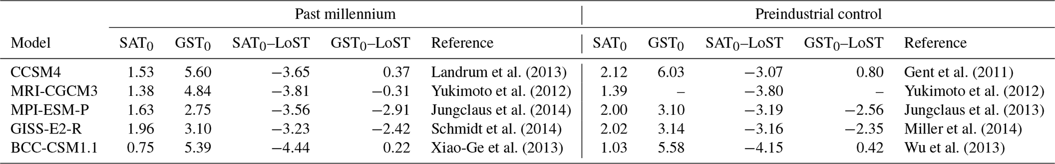
We use five past millennium (PM) and five preindustrial control (piControl) GCM simulations (see Table 1 for references) from the third phase of the Paleoclimate Modelling Intercomparison Project and the fifth phase of the Coupled Model Intercomparison Project (PMIP3/CMIP5) (Braconnot et al., 2012; Taylor et al., 2011) to test the LoST database. PM simulations (Past1000 experiment in the PMIP3/CMIP5 database) simulate the climate response to prescribed external forcings from Schmidt et al. (2011) for the period from 850 to 1850 CE, including orbital variations, changes in solar activity, greenhouse gas concentrations, volcanic eruptions and changes in land use and land cover. Each PMIP3/CMIP5 GCM also performs a piControl simulation forced with agreed preindustrial forcings to provide a baseline from which to start transient climate experiments. For more details about the PMIP3/CMIP5 control simulations and initialization procedures see Sen Gupta et al. (2013) and Séférian et al. (2016).

Landrum et al. (2013)Gent et al. (2011)Yukimoto et al. (2012)Yukimoto et al. (2012)Jungclaus et al. (2014)Jungclaus et al. (2013)Schmidt et al. (2014)Miller et al. (2014)Xiao-Ge et al. (2013)Wu et al. (2013)

Table 1 Model name, SAT₀ estimates, GST₀ estimates, SAT₀ and GST₀ differences with the mean LoST temperatures and references for each PMIP3/CMIP5 GCM simulation. All results are in degrees Celsius. Ground temperatures for the MRI-CGCM3 piControl simulation could not be retrieved from the PMIP3/CMIP5 data servers. The temperature average of the LoST database is 5.2^∘C, with a 95 % confidence interval between 5.0 and 5.4 ^∘C.

2.3 Borehole data

Here, we use estimates of long-term surface temperatures from the database described in Jaume-Santero et al. (2016). The BTP measurements of this database have been previously filtered excluding profiles with non-climatic signals and artifacts, thus providing 514 BTPs suitable for climate studies over North America. The standard methodology to retrieve past temperature and flux histories from geothermal data assumes that each borehole temperature profile results from the superposition of a transient perturbation due to the changes in the surface energy balance with time and the quasi-steady state of the subsurface thermal regime (e.g., Huang et al., 2000; Harris and Chapman, 2001; Beltrami, 2002). Therefore, considering the subsurface as a half space without heat production from radioactive decay or advection, the solution of the heat diffusion equation for a temperature profile can be approximated as follows (e.g., Jaume-Santero et al., 2016):

$$\begin{array}{}\text{(1)}& T\left(z\right)=T_{\mathrm{0}}+q_{\mathrm{0}}\cdot R\left(z\right)+T_{\mathrm{t}}\left(t\right),\end{array}$$

where T_t is the surface transient perturbation, T₀ is the long-term surface temperature (T₀ temperature hereafter), q₀ is the subsurface flux at equilibrium and R(z) is the thermal resistance (Bullard and Schonland, 1939). Estimates of thermal resistance require measurements of thermal conductivity through the subsurface profile, but the majority of BTPs available does not present such conductivity data. Thus, the thermal conductivity is assumed to be constant and Eq. (1) is rewritten as

$$\begin{array}{}\text{(2)}& T\left(z\right)=T_{\mathrm{0}}+\mathrm{\Gamma }\cdot z+T_{\mathrm{t}}\left(t\right),\end{array}$$

where Γ is the subsurface thermal gradient at equilibrium. The recorded surface transient perturbation (T_t) can be retrieved from each temperature profile, once the subsurface thermal equilibrium is estimated (for more details about the borehole methodology, see Mareschal and Beltrami, 1992; Bodri and Cermak, 2007; Jaume-Santero et al., 2016). As the heat flux from the Earth's interior remains stable at timescales of millions of years and the deepest part of a BTP is the least affected by the recent changes in the surface energy balance, the quasi-equilibrium state of the subsurface thermal regime can be estimated from the deepest temperatures of each borehole profile (see scheme in Fig. 1). Once vertical variations in the thermal properties of the subsurface rocks are taken into account, temperature depends linearly on depth at the bottom part of the temperature profile, allowing for the approximation of the subsurface thermal equilibrium by a regression. The extrapolation of this linear behavior to the surface can be interpreted as the long-term mean surface temperature at each borehole location (T₀ temperature in Eq. 2 and Fig. 1, see Pickler et al., 2016, for further details). Depending on the profile's depth, the T₀ temperatures represent the long-term ground surface temperature for a determined period of time. Due to the nature of heat diffusion through the ground, the required time (t) for a change in the surface energy balance to reach a certain depth (z) is given by the following equation (Carslaw and Jaeger, 1959; Pickler et al., 2016):

$$\begin{array}{}\text{(3)}& t\approx {\displaystyle \frac{z^{\mathrm{2}}}{\mathrm{4}\mathit{\kappa }}},\end{array}$$

where κ is the thermal diffusivity of the subsurface. We consider $\mathit{\kappa }=\mathrm{1}\times {\mathrm{10}}^{-\mathrm{6}}$ m² s⁻¹ for all BTP measurements (Cermak and Rybach, 1982). In this study, all BTPs are truncated at the same depth (300 m) to ensure that all T₀ temperatures are estimated for the same temporal period. We use the last 100 m of each BTP to estimate the subsurface thermal equilibrium, obtaining an estimated temporal period that approximately ranges from ∼1300 CE (z=300 m) to ∼1700 CE (z=200 m). Hence, this period of time provides a baseline to compare with long-term temperatures from the PMIP3/CMIP5 PM simulations. However, the estimated temporal period is not homogeneous as result of the nonlinear relationship between time and depth (Beltrami and Mareschal, 1995); thus, the estimates of recent years (i.e., 1700 CE) are better determined than the estimates of past years (1300 CE). Influences of long-term perturbations of the past surface energy budget outside of this temporal window may also affect the temperature within the depth range used here (see Sect. 5 for more details).

Figure 1 Synthetic borehole temperature profile (black dots) using data from the CCSM4 PM simulation (inset) and the linear fit of temperatures between 200 and 300 m (red line). The synthetic temperature profile is generated using the simulated global ground temperature anomaly at a depth of 1.0 m for the period from 1300 to 1700 CE as the transient perturbation (T_t), mean ground temperature as the long-term surface temperature (T₀) and a typical thermal gradient (Γ) of 0.01 K m⁻¹ (Jaume-Santero et al., 2016). The equivalence between depth (z) and time (t) is given by Eq. (3). Thermal diffusivity is considered as $\mathit{\kappa }=\mathrm{1}\times {\mathrm{10}}^{-\mathrm{6}}$ m² s⁻¹ (Cermak and Rybach, 1982).

3 The LoST database

In order to provide a gridded dataset over continental North America, T₀ temperatures from BTP measurements are spatially interpolated to a 0.5^∘ × 0.5^∘ grid using the gradient plus inverse distance squared (GIDS) technique. The GIDS method (Nalder and Wein, 1998) relies on the multiple linear regression of observed climate variables to retrieve longitudinal, latitudinal and altitudinal gradients that are employed to estimate values for gridded nodes. The contribution of each measurement is inverse-weighted by their squared distance to the target node, while the coefficients from the regression analysis allow to correct for the location of each measurement:

$$\begin{array}{}\text{(4)}& \begin{array}{rl}{V}_{\mathrm{0}}& ={\displaystyle \frac{\mathrm{1}}{{\sum }_{i=\mathrm{1}}^N{d}_i^{-\mathrm{2}}}}\left[\sum _i^N\left\{V_i+({\mathrm{lat}}_{\mathrm{0}}-{\mathrm{lat}}_i)C_{\mathrm{lat}}\right.\right.\\ & \left.\left.+({\mathrm{long}}_{\mathrm{0}}-{\mathrm{long}}_i)C_{\mathrm{long}}+(z_{\mathrm{0}}-z_i)C_z\right\}{d}_i^{-\mathrm{2}}\right],\end{array}\end{array}$$

where V₀ is the predicted variable at the target node, V_i; lat_i, long_i and z_i represent the variable, latitude, longitude and altitude of the ith measurement respectively; lat₀, long₀ and z₀ represent the latitude, longitude and altitude of the target node respectively; C_lat, C_long and C_z are the coefficients from the regression analysis; and d_i is the distance from the ith measurement to the target node. The propagation of known errors in the GIDS algorithm is described in Sect. S1 in the Supplement. The GIDS technique has been used to interpolate surface temperature, precipitation, evapotranspiration and other climate variables in several zones of the world including North America (e.g., Price et al., 2000; Mardikis et al., 2005). Furthermore, the GIDS method performs well in comparison with other broadly used interpolation techniques like co-kriging or smoothing splines (ANUSPLIN suite) (Nalder and Wein, 1998; Price et al., 2000; Li and Heap, 2011), and it has been previously employed to downscale CMIP5 simulations (McCullough et al., 2016).

As the T₀ dataset employed here provides latitudes and longitudes for each temperature profile, we expand the database estimating the altitude above sea level for each BTP measurement from the second version of the 2 min Gridded Global Relief Data (ETOPO2 v2) of the National Oceanic and Atmospheric Administration (National Geophysical Data Center, 2006; Two-minute Gridded Global Relief Data, NOAA, https://doi.org/10.7289/V5J1012Q, last access: on 7 July 2017). For this study, the regression analysis of T₀ temperatures considering latitude, longitude and altitude yields robust results, with an R² value of 0.865 and a p value of ≪0.05. The distance from the measurements to the nodes is computed using the Vincenty formula for an ellipsoid with different major and minor axes (Vincenty, 1975); therefore, the altitude of both measurements and grid nodes are not considered in our distance calculations.

We performed a pseudo-proxy experiment (e.g., Smerdon, 2012) to determine the maximum appropriate distance from a grid node to a BTP measurement to interpolate the T₀ temperatures. That is, we used the long-term mean ground surface temperatures for the period from 1300 to 1700 CE from the five PMIP3/CMIP5 PM simulations as surrogate realities, and applied the interpolation methodology employed to create the LoST database. Therefore, these GCM simulations were regridded to a 0.5^∘ × 0.5^∘ grid, considering grid cells containing BTP measurements as a reference for applying Eq. (4) to the rest of grid cells. Then, root-mean-squared errors (RMSEs) between the interpolated data and the remapped simulations were computed (Fig. S1 in the Supplement). We set 650 km as the maximum distance criterion as this is the maximum distance at which the RMSE is lower than 1.0 ^∘C for the five simulations. Nevertheless, such a distance criterion produces results for three grid cells in the Yucatán Peninsula (Mexico), which we consider unjustifiable as there are no BTP measurements in or near this part of Mexico. Therefore, these grid cells are masked out from our analysis.

4 Results

The distribution of LoST temperatures at grid cells containing BTP measurements reproduces the shape of the distribution of raw T₀ temperatures (Fig. 2a), indicating that the GIDS interpolation does not substantially modify the shape of the original distribution of temperatures retrieved from BTP measurements. However, the distribution of the entire LoST database resembles the distribution of CRU temperatures, differing from the distribution of the raw T₀ temperatures. This change in the temperature distribution after the spatial interpolation may be related to the inclusion of interpolated temperatures at higher and lower latitudes than for the raw T₀ temperatures, as the majority of BTP measurements cover from 35 to 60^∘ N. Nonetheless, the latitudinal mean temperatures from the LoST database are consistent with T₀ temperatures from BTP measurements, either considering only grid cells with BTP measurements or the entire LoST database (Fig. 2b). The latitudinal mean temperatures from the LoST database reach higher values than the CRU database at latitudes higher than ∼50^∘ N, whereas both datasets achieve similar mean temperatures at lower latitudes (Fig. 2b). Previous studies have found warmer ground temperatures than air temperatures in meteorological observations over North America, which is probably due to the insulating effect of snow cover during winter (e.g., Beltrami and Kellman, 2003; Smerdon et al., 2003). That is, warmer temperatures should be expected for the LoST database than for the CRU database, as our results show (Fig. 2a and b). Nevertheless, it should be noted that the CRU database covers a period with a marked global temperature increase (Hartmann et al., 2013). Therefore, estimates of long-term surface temperatures from CRU data reflect such a temperature increase, hindering the direct comparison between both datasets. Despite this difference in the climatology of both databases, the long-term surface temperature from the LoST dataset reproduces the expected spatial pattern of temperatures for North America (Fig. 2c, d), which is in agreement with long-term surface temperatures estimated from BTP measurements and with long-term surface temperatures from CRU data.

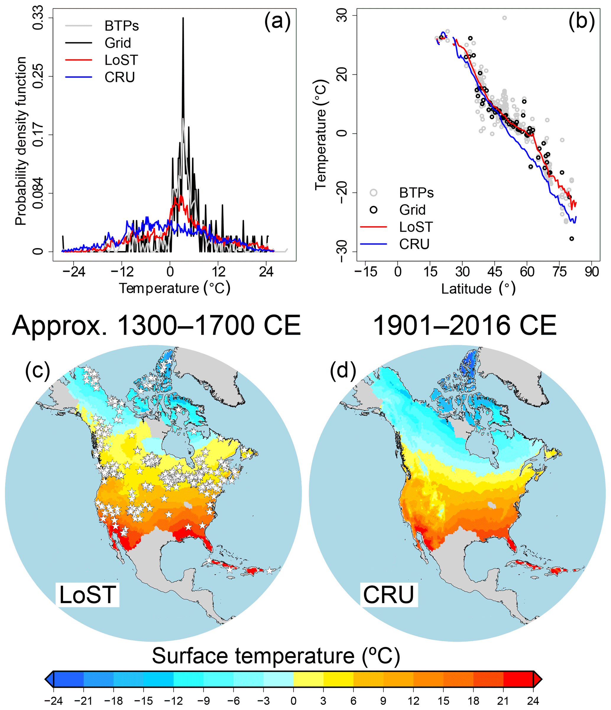
Figure 2 Histogram (a) and latitudinal mean temperatures (b) from BTP measurements (gray), LoST temperatures at grid cells containing BTP measurements (black), LoST temperatures (red) and mean surface air temperature from the CRU database (blue). LoST temperatures (∼1300–1700 CE) (c) compared with the mean surface air temperature from CRU data (1901–2015 CE) (d). White stars in (c) indicate the locations of the 514 BTP measurements.

The LoST temperatures were also compared with long-term surface temperature estimates from five past millennium (PM) and five piControl simulations (Table 1) included in the PMIP3/CMIP5 archive to test the realism of forced and control GCM simulations in reproducing estimates of long-term surface temperatures. Long-term surface temperatures from the PM simulations are estimated as the mean surface air temperature for the period from 1300 to 1700 CE (SAT₀) and the mean ground surface temperature linearly interpolated at 1.0 m depth for the same period (GST₀), in order to be consistent with the estimated temporal range for T₀ temperatures in Sect. 2.3. The PMIP3/CMIP5 simulations are interpolated onto the grid of the LoST database; SAT₀ and GST₀ values are only estimated at grid cells containing LoST temperatures. SAT₀ and GST₀ values are also estimated for piControl simulations following the same method, but averaging over each entire control simulation.

Surface temperatures from PMIP3/CMIP5 PM and piControl simulations show similar latitudinal patterns to that from the LoST database, with lower temperatures at northern latitudes and higher temperatures at southern latitudes (Figs. S2, S3). SAT₀ estimates from the CCSM4, the MRI-CGCM3 and the BCC-CSM1.1 models show generally lower values than LoST temperatures for both piControl and PM simulations, whereas GST₀ estimates show higher values than LoST temperatures at high latitudes for the same GCM simulations (Figs. S4, S5). Such results are in agreement with previous analyses of the air and ground temperature relationship within GCM simulations (González-Rouco et al., 2003, 2006; Stieglitz and Smerdon, 2007; Koven et al., 2013; García-García et al., 2016) and meteorological observations over North America (e.g., Smerdon et al., 2003; Beltrami and Kellman, 2003). In contrast, MPI-ESM-P and GISS-E2-R simulations present lower SAT₀ and GST₀ values than LoST temperatures, indicating lower long-term ground surface temperatures than the rest of the models (Table 1; Figs. S4, S5). The comparison of the mean LoST temperature over North America with the simulated temperature evolution by each GCM shows three different behaviors within the PMIP3/CMIP5 ensemble. The CCSM4 and the BCC-CSM1.1 simulations present lower mean air temperatures and higher mean ground temperatures than the mean LoST temperature (Fig. 3, Table 1). The similar GST₀ and mean ground surface temperatures for the CCSM4 and the BCC-CSM1.1 GCMs in both PM and piControl simulations were expected as these models use a similar land surface model component (Wu et al., 2014), and the simulated ground temperatures by CMIP5 models are highly dependent on the land surface model component employed (García-García et al., 2019; Slater and Lawrence, 2013). In contrast, the GISS-E2-R and the MPI-ESM-P models produce lower mean GST₀ values than the mean LoST temperature and the rest of models, while simulating similar SAT₀ values to those from the rest of the PMIP3/CMIP5 GCMs. Previous results have shown that the MPI-ESM-P PM simulation yields a high air–ground temperature coupling (García-García et al., 2016), probably due to the omission of latent heat of fusion in soil water (Koven et al., 2013). This could cause the low ground surface temperature simulated by the MPI-ESM-P model in both PM and piControl simulations in comparison with the mean LoST temperature (Fig. 3). A strong air–ground coupling may also cause the low ground surface temperature in the GISS-E2-R simulations, as the magnitude of the difference between GST₀ and SAT₀ is similar to that from the MPI-ESM-P simulations (Table 1). Finally, the MRI-CGCM3 PM simulation yields GST₀ values below the LoST climatology, but only by 0.3 ^∘C (0.1 ^∘C if considering the 2σ range of the LoST climatology, Fig. S6), which are relatively small in comparison with the differences between the LoST climatology and the GST₀ values from the MPI-ESM-P and GISS-E2-R simulations (>2.0 ^∘C, Table 1). Thus, we can consider that three of the five PMIP3/CMIP5 GCMs (the CCSM4, the MRI-CGCM3 and the BCC-CSM1.1) simulate a surface temperature climatology, in the PM (1300–1700 CE) and piControl simulations, comparable to that from the LoST dataset, which is an unexpected result as none of the PMIP3/CMIP5 GCM simulations studied here were specifically tuned to match this climatology.

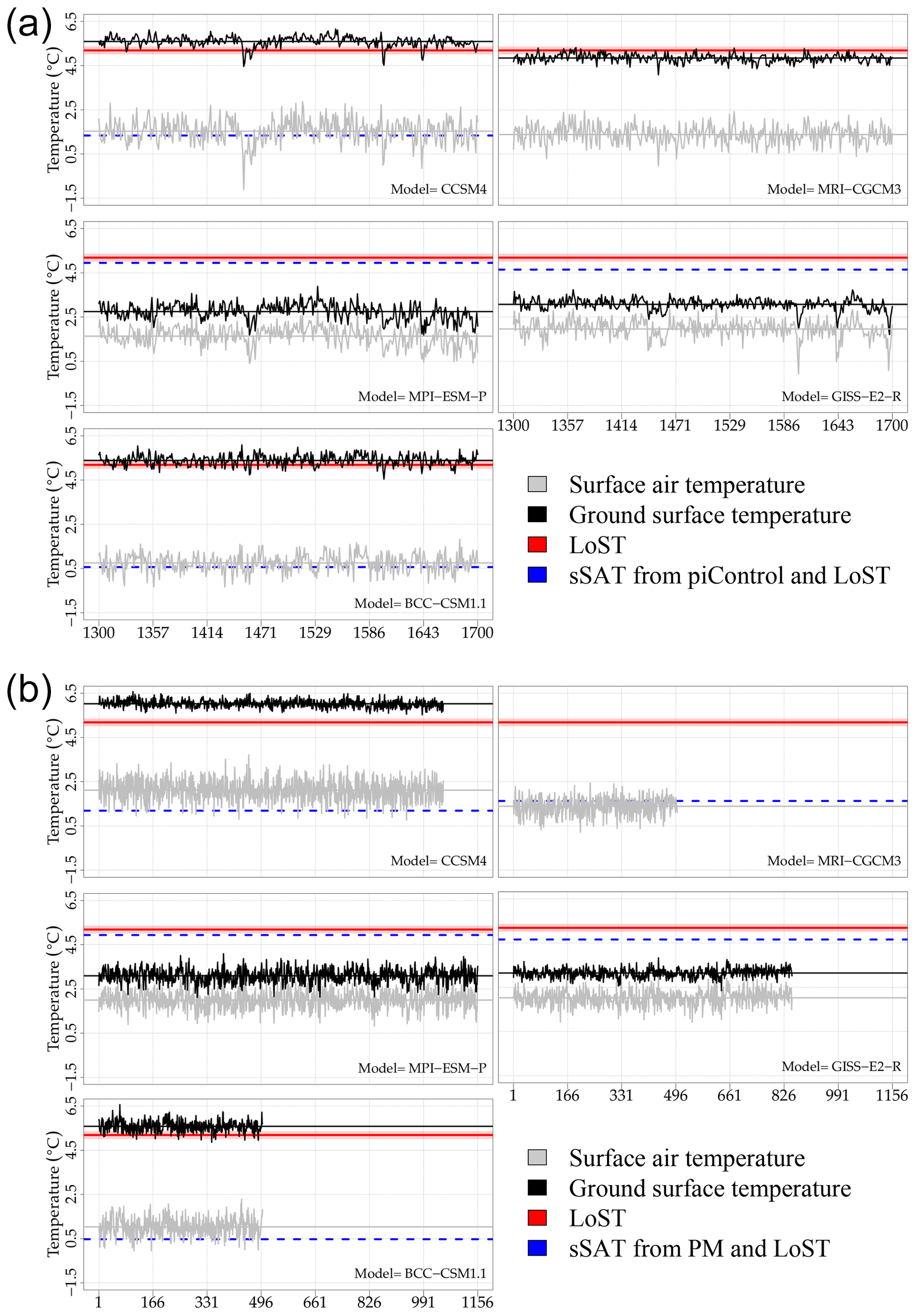
Figure 3 Surface air temperature evolution (gray solid line), ground surface temperature evolution (black solid line), SAT₀ (gray horizontal line) and GST₀ (black horizontal line) for (a) PMIP3/CMIP5 PM and (b) PMIP3/CMIP5 piControl simulations. Solid red lines represent the mean LoST temperature, and the red shadow represents the 95 % confidence interval (Sect. S1, Fig. S6). Dashed blue lines represent estimated references for long-term surface air temperatures from the LoST climatology and the simulated air–ground temperature offset in (a) piControl and (b) PM simulations. Ground temperatures for the MRI-CGCM3 piControl simulation could not be retrieved from the PMIP3/CMIP5 data servers.

5 Discussion

Our results demonstrate that LoST temperatures can be used as a reference for assessing the represented climatology in both PM and piControl simulations. Nevertheless, the determination of T₀ temperatures presents some uncertainties that should be discussed. The extrapolation of each quasi-equilibrium temperature profile to the surface introduces a small error in the LoST estimates, averaging less than 0.15 ^∘C from the 514 BTPs evaluated here (see Sect. S1 for details about the error treatment in the LoST database). Rock heterogeneity should also be considered for estimating T₀ temperatures. We assume homogenous thermal properties for all borehole profiles, which is another source of uncertainty for LoST temperatures. The ideal approach consists of estimating the thermal resistance with depth (Eq. 1), but the absence of thermal conductivity measurements for the BTPs employed (Jaume-Santero et al., 2016) makes this approach impractical. Additionally, measurements of thermal conductivity tend to be distributed around a central value (e.g., the measurements at the Neil Well, Beltrami and Taylor, 1995). If the thermal conductivity varies systematically with depth at a certain location, such variation will be reflected in the temperature profile as an unphysical signal. Such logs were removed from the database employed in this analysis, as explained in Jaume-Santero et al. (2016). Therefore, it is reasonable to assume a homogenous conductivity with depth. Long-term alterations of the surface energy balance out of the 1300–1700 CE period may also affect the LoST estimates. Particularly, possible transient temperatures in BTPs due to the Little Ice Age (LIA) and the Medieval Warm Period (MWP) add a certain degree of uncertainty in the determination of T₀ values. However, the spatial extent of both the LIA and the MWP was not homogeneous over North America (e.g., Masson-Delmotte et al., 2013, and references therein), meaning that not all BTPs were affected by the events (Beltrami and Mareschal, 1992; Chouinard et al., 2007; Jaume-Santero et al., 2016). Additionally, the influence of the LIA and the MWP should be part of any millennial-scale transient climate simulation; therefore, the effect of such climate events is taken into account in the comparison between LoST results and transient climate simulations. The absence of these two periods in piControl simulations probably contributes to the slightly poorer agreement between LoST temperatures and piControl temperatures in comparison with results for the PM simulation (Fig. 3). Another factor that may impact the retrieved quasi-equilibrium temperature profile is the heterogeneity of North American topography (e.g., Kohl, 1999). To our knowledge, all analyzed BTPs are located in plain terrain, and were not corrected for elevation as the BTP database employed does not provide elevation data. Therefore, we use the ETOPO2 database to assess if the altitude distribution of the BTPs is sufficient to represent the topography of the LoST domain. The altitude distribution over the LoST domain and at grid cells containing borehole sites are displayed in Fig. S8. Both histograms present a similar shape for altitudes up to ∼430 m, showing a lack of borehole locations at altitudes between ∼430 and ∼1013 m. The uneven latitudinal distribution of borehole sites probably causes this gap in the distribution of altitudes, as well as a small excess of BTP locations at high altitudes. Despite these differences, both distributions are generally in agreement, indicating a sufficient altitude distribution from the borehole database to represent the North American broad-scale topography.

There are, however, two main limitations for the application of the LoST database at this stage of the study: the supplied variable and the regional character of the database. The LoST database is constituted by estimates of long-term ground surface temperatures, whereas GCM simulations are typically evaluated against observations of surface air temperature (SAT) (e.g., Mauritsen et al., 2012; Flato et al., 2013; Séférian et al., 2016; Schmidt et al., 2017). We can provide a reference for simulated long-term SAT by accounting for the offset between simulated air and ground temperatures and using the LoST temperatures (synthetic SAT, sSAT). As an example, SAT references are estimated for the five PM and five piControl simulations employed in this study (dashed blue line in Fig. 3). SAT references for PM simulations are estimated from the offset between air and ground temperatures in piControl simulations, whereas SAT references for piControl simulations are estimated from the offset between air and ground temperatures in PM simulations. Such offsets show a constant behavior in both simulations (Fig. S7). GCM simulations in disagreement with the estimated SAT reference (the MPI-ESM-P and the GISS-E2-R simulations) may represent a strong air–ground coupling, as discussed in Sect. 4. Therefore, although the LoST database contains estimates of ground surface temperatures, it may also be used to assess simulated long-term surface air temperatures as a first-order approach.

The regional character of the LoST database presented poses some caveats for analyzing the global climatology of preindustrial simulations. Indeed, results of the simulated regional climatology cannot be globally extrapolated as the magnitude of the potential spurious drifts in control simulations varies markedly at regional scales and these regional drifts could be larger than the global-averaged drift (Sen Gupta et al., 2012, 2013). Further work would consist of generating a global LoST database from the existing global network of BTP measurements, which would help to minimize the effect of possible regional drifts on the simulated climatology. However, BTP measurements are scarce in the Southern Hemisphere, which is a potential burden that needs to be considered when assembling a global version of this database. Additionally, the temperature profiles employed in this study to estimate T₀ temperatures were truncated to a depth of 300 m, which determines the temporal period of reference for the comparison with PM simulations. Deeper BTP measurements can retrieve the climatology of previous time periods, although the global BTP network contains fewer temperature profiles deeper than 300 m (see Fig. 1 in Beltrami et al., 2015).

Despite the regional character of the LoST temperatures, the northern BTPs contained in this database allow for the evaluation of the long-term stability of permafrost over North America. That is, the northern temperatures in this database can be compared with regional and global simulations as a reference to the preindustrial permafrost stability. Furthermore, previous studies have found that the CMIP5 GCM simulations have difficulties properly representing permafrost evolution (Koven et al., 2013; Slater and Lawrence, 2013), partially due to the broad range of simulated climate trajectories by each GCM and the differences between the land surface model components employed (Slater and Lawrence, 2013). Using LoST temperatures to improve the surface temperature climatology of global and regional simulations may enhance the simulated long-term preindustrial 0 ^∘C isotherm, which is important to correctly represent permafrost evolution.

Numerous proxy-data-based reconstructions of temperature, precipitation and other climate related variables exist for North America, providing a reference for the evaluation of important aspects of past and future climate model simulations (e.g., PAGES 2k-PMIP3 Group, 2015; Cook et al., 2015). Proxy-data temperature reconstructions have already been compared against borehole temperature records of past variations in surface temperature over North America (e.g., Jaume-Santero et al., 2016). It is worthy to note that proxy systems are indirect sources of climate information requiring a calibration procedure with modern meteorological data, whereas borehole temperature data consist of direct measurements of the thermal regime of the subsurface in the recent past. That is, the LoST database contains information derived from direct measurements of subsurface temperatures, constituting the first estimates of long-term absolute surface temperatures in North America. Another important difference between proxy and borehole reconstructions is that most proxy systems generally capture high-frequency variations of climate conditions (Moberg et al., 2005), whereas borehole temperature profiles record long-term changes in the surface conditions, filtering out short-period signals. In this context, LoST temperatures provide a complementary reference to the multiproxy database over North America for evaluating the performance of climate model simulations.

6 Conclusions

A gridded database of past long-term surface temperatures over most parts of continental North America has been assembled from geothermal measurements. Our results show that this database can be used as a reference to evaluate the realism of GCM preindustrial control and past millennium simulations and possibly to improve the reference climate state by adjusting key parameters or preindustrial forcings in control experiments. Hence, the spread in ECS estimates by GCM simulations may be reduced given the relationship between control temperature climatology and three long-term powerful feedbacks: the ice–albedo feedback, the water vapor feedback and the permafrost–carbon feedback. Future work would consist of generating a global version of the LoST database using the rest of the global network of borehole temperature profile measurements and following the described methodology, as well as generating new versions of this global database including future temperature profile measurements.