the Creative Commons Attribution 4.0 License.
the Creative Commons Attribution 4.0 License.
 | 16 Aug 2018
Deglacial carbon cycle changes observed in a compilation of 127 benthic δ13C time series (20–6 ka)
Carlye D. Peterson
Lorraine E. Lisiecki
We present a compilation of 127 time series δ13C records from Cibicides wuellerstorfi spanning the last deglaciation (20–6 ka) which is well-suited for reconstructing large-scale carbon cycle changes, especially for comparison with isotope-enabled carbon cycle models. The age models for the δ13C records are derived from regional planktic radiocarbon compilations (Stern and Lisiecki, 2014). The δ13C records were stacked in nine different regions and then combined using volume-weighted averages to create intermediate, deep, and global δ13C stacks. These benthic δ13C stacks are used to reconstruct changes in the size of the terrestrial biosphere and deep ocean carbon storage. The timing of change in global mean δ13C is interpreted to indicate terrestrial biosphere expansion from 19–6 ka. The δ13C gradient between the intermediate and deep ocean, which we interpret as a proxy for deep ocean carbon storage, matches the pattern of atmospheric CO2 change observed in ice core records. The presence of signals associated with the terrestrial biosphere and atmospheric CO2 indicates that the compiled δ13C records have sufficient spatial coverage and time resolution to accurately reconstruct large-scale carbon cycle changes during the glacial termination.
- Article
(3101 KB) - Full-text XML
-
Supplement
(3414 KB) - BibTeX
- EndNote


On glacial–interglacial timescales, carbon cycle changes redistribute the amount of carbon stored in the deep ocean, atmosphere, and terrestrial biosphere (e.g., Broecker, 1982; Siegenthaler et al., 2005). For example, as atmospheric CO2 increased across the deglaciation, atmospheric δ13C decreased, likely due to the ventilation of respired 13C-depleted carbon from the deep ocean (e.g., Schmitt et al., 2012; Eggleston et al., 2016). However, identifying the biogeochemical mechanisms associated with these carbon transfers is complicated by a variety of carbon cycle feedbacks (e.g., Archer et al., 2000; Sigman and Boyle, 2000; Peacock et al., 2006; Toggweiler et al., 2006; Kohfeld and Ridgwell, 2009; Brovkin et al., 2012; Menviel et al., 2012; Galbraith and Jaccard, 2015; Buchanan et al., 2016). This study seeks to improve our understanding of glacial–interglacial carbon cycle changes by reconstructing changes in mean ocean δ13C and its vertical gradient and comparing the results with changes in the terrestrial biosphere and atmospheric CO2.
The δ13C of benthic foraminiferal calcite is a well-established carbon cycle proxy, which records the δ13C signature of dissolved inorganic carbon (DIC) in seawater at seafloor depths (e.g., Woodruff and Savin, 1985; Zahn et al., 1986; Lutze and Thiel, 1989; Duplessy et al., 1988; Mackensen, 2008; Gottschalk et al., 2016; Schmittner et al., 2017). Averages of benthic foraminiferal δ13C time series, called stacks, can improve the signal-to-noise ratio of regional or global seawater changes (e.g., Lisiecki et al., 2008; Lisiecki, 2014). Global mean benthic δ13C change is likely caused by changes in terrestrial organic carbon storage (Shackleton, 1977; Curry et al., 1988; Duplessy et al., 1988; Ciais et al., 2012; Peterson et al., 2014), while vertical δ13C gradients may record changes in deep ocean carbon storage and atmospheric CO2 (Oppo and Fairbanks, 1990; Flower et al., 2000; Hodell et al., 2003b; Lisiecki, 2010). The vertical δ13C gradient between the surface (high δ13C) and deep ocean (low δ13C) primarily results from the accumulation of low-δ13C-respired organic carbon in deep water, which temporarily sequesters it from the atmosphere. Conversely, vertical mixing of the ocean will tend to ventilate deep ocean carbon to the surface ocean and atmosphere while simultaneously decreasing the vertical δ13C gradient. Therefore, the vertical δ13C gradient likely records changes in deep ocean carbon storage, which is an important factor controlling glacial–interglacial changes in atmospheric CO2 (e.g., Schmitt et al., 2012; Eggleston et al., 2016).
Here we compile and analyze 127 high-resolution benthic δ13C records from the Atlantic, Pacific, and Indian oceans spanning the last deglaciation to investigate changes in both the ocean and terrestrial biosphere components of the global carbon cycle. Benthic δ13C records are combined into regional stacks, which are then used to construct time series of volume-weighted global mean δ13C and the vertical δ13C gradient between intermediate and deep waters.
We analyze these stacks to test the following hypotheses:
-
The deglacial pattern of global mean ocean δ13C change is a proxy for changes in the size of the terrestrial biosphere. If so, global mean δ13C should continue to increase after atmospheric CO2 levels plateau at 11 ka due to the slower response times for ice sheet retreat and ecosystem change (e.g., Hoogakker et al., 2016; Davies-Barnard et al., 2017). We compare the reconstructed global mean δ13C change with several carbon cycle model estimates of terrestrial biosphere change. Additionally, we evaluate whether deep Pacific δ13C correlates with global mean δ13C change as previously assumed (Shackleton et al., 1983; Curry and Oppo, 1997; Lisiecki et al., 2008). This study provides the first opportunity to compare time series of deep Pacific δ13C with a volume-weighted global mean δ13C stack.
-
Changes in the vertical δ13C gradient should closely resemble time series of atmospheric CO2 if the deglacial CO2 increase is caused by a decrease in deep ocean carbon storage. This hypothesis is supported by findings on orbital timescales using a smaller number of sites (Oppo and Fairbanks, 1990; Flower et al., 2000; Hodell et al., 2003b; Lisiecki, 2010), but the link between the vertical δ13C gradient and CO2 has not yet been evaluated at millennial timescales or using a global data compilation. Observing such a link would improve our understanding of deglacial atmospheric CO2 increase and, furthermore, demonstrate that the data compilation presented here has adequate spatial and temporal resolution with sufficiently precise age models to reconstruct millennial-scale changes in the global carbon cycle.
2.1 Benthic δ13C reconstructions
Measurements of δ13C from the calcite tests of epibenthic foraminifera Cibicides wuellerstorfi and related species (Schweizer et al., 2009) are commonly used to trace the spatial distribution of nutrients and deep water masses as well as changes in ocean carbon cycling (e.g., Curry et al., 1988; Duplessy et al., 1988; Curry and Oppo, 2005; Schmittner et al., 2017). Benthic δ13C is also slightly influenced (<15 %) by changes in carbonate ion concentration of sea water (Schmittner et al., 2017). Additionally, the Cibicides species C. kullenbergi and C. mundulus, often measured in deep South Atlantic cores, appear to record more depleted δ13C values than C. wuellerstorfi (Gottschalk et al., 2016).
Mean δ13C has been estimated for the Last Glacial Maximum (LGM, 20 ka) and Late Holocene (6–0 ka) using global compilations of Cibicides wuellerstorfi δ13C records (e.g., Shackleton, 1977; Duplessy et al., 1988; Curry et al., 1988; Boyle, 1992; Matsumoto and Lynch-Stieglitz, 1999; Curry and Oppo, 2005; Herguera et al., 2010; Oliver et al., 2010; Hesse et al., 2011; Peterson et al., 2014; Gebbie et al., 2015). These time slice studies include as many as 500 core sites, but generally undersample portions of the ocean with poor carbonate preservation, low primary productivity, and low sedimentation rates (i.e., the Southern Ocean south of 55∘ S, the Indian Ocean, and the Pacific Ocean). In contrast, some portions of the Atlantic, especially the North Atlantic, are relatively well-sampled with abundant, well-preserved C. wuellerstorfi. Therefore, whole-ocean mean δ13C change is less well-constrained than Atlantic δ13C.
Because deglacial carbon cycle changes occurred on millennial to centennial timescales (Marcott et al., 2014), observing these changes in the ocean requires a global compilation of high-resolution benthic δ13C time series on a consistent age model across the glacial termination. Previous global compilations of δ13C time series focus on orbital-scale responses because their age models are not precise enough to analyze the relative timing of carbon cycle changes during the deglaciation (e.g., Lisiecki et al., 2008). For example, Oliver et al. (2010) caution that their global δ13C data synthesis, which includes 258 records from many benthic and planktic foraminifera species, should not be used to analyze δ13C changes on timescales of less than 10 kyr due to age model uncertainty and the inclusion of low-resolution records. Instead, studies of δ13C change across the last glacial termination often use local or regional depth transects that contain high-resolution δ13C records with good age control (e.g., Sarnthein et al., 1994; Thornalley et al., 2010; Hoffman and Lund, 2012; Tessin and Lund, 2013; Lund et al., 2015; Oppo et al., 2015; Sikes et al., 2016). In modeling studies, transient simulations are typically compared to a small number of individual benthic δ13C records or regional syntheses, presumably due to the limitations of available global δ13C compilations (e.g., Köhler et al., 2005, 2010; Brovkin et al., 2007).
2.2 Terrestrial biosphere and mean ocean δ13C
A portion of the additional carbon released from the deep ocean since the LGM was taken up by the terrestrial biosphere. The transfer of carbon between the terrestrial biosphere and the deep ocean affects the global mean value of benthic δ13C because the mean δ13C signature of the terrestrial biosphere is significantly more negative (approximately −25 ‰) than mean ocean δ13C (approximately 0 ‰) (Shackleton, 1977). The change in global mean benthic δ13C between the LGM and the Holocene is estimated to be 0.32 ‰ ± 0.20 ‰ (Peterson et al., 2014; Gebbie et al., 2015), but the timing of mean benthic δ13C change across the deglaciation is not well known.
The amount of terrestrial carbon storage change (soils and vegetation) can be reconstructed in many ways, including terrestrial vegetation proxies and archives (e.g., pollen, paleovegetation); carbon cycle models (e.g., box models, inverse methods, dynamic global vegetation models, biomization methods, etc.); and proxies such as benthic δ13C, triple oxygen isotopes (Landais et al., 2007), and atmospheric carbonyl sulfide (Aydin et al., 2016). These methods produce estimates of change in terrestrial carbon storage between the LGM and Holocene varying from 200–1900 PgC due to uncertainties and assumptions associated with each method (see discussion and citations within Peterson et al., 2014).
Due to uncertainties in the total magnitude of change, here we focus on comparing the timing of changes in terrestrial carbon storage and global mean benthic δ13C. Models simulate rapid increases in terrestrial carbon storage from approximately 19–10 ka, followed by more gradual changes from 10–0 ka (Kaplan et al., 2002; Joos et al., 2004; Köhler et al., 2005). More recently, the potential effects of changes in poorly constrained carbon reservoirs (e.g., beneath ice sheets and on continental shelves) were evaluated using deglacial simulations of biogeophysical and land carbon changes from the HadCM3 general circulation model (GCM). The model simulated a rapid increase in terrestrial carbon storage from 20–14 ka, different responses between 14–11 ka depending on the model scenario, and then steady, gradual change from 11–4 ka (Davies-Barnard et al., 2017).
Estimates of global mean benthic δ13C are also used to remove global changes from individual δ13C records to identify patterns of local or regional change, e.g., related to ocean circulation. Because estimates of global mean δ13C have only been available for the LGM and Holocene, some studies use deep Pacific δ13C time series as a proxy for global mean δ13C change (Shackleton et al., 1983; Curry and Oppo, 1997; Lisiecki et al., 2008). Given the large volume and carbon storage capacity of the deep Pacific, its δ13C change should be similar in magnitude and timing to the mean ocean δ13C change; however, no study has yet confirmed this relationship. For example, low sedimentation rates and poor carbonate preservation in the deep Pacific may limit how well deep Pacific δ13C time series resolve changes in mean ocean δ13C. Additionally, large changes in Atlantic or Indian Ocean δ13C could alter the timing of global mean δ13C relative to the Pacific. By constructing a global benthic δ13C stack, we can now directly compare deep Pacific δ13C with global mean δ13C change across the deglaciation.
2.3 Vertical gradients in benthic δ13C
A vertical gradient in the δ13C of DIC between surface-to-intermediate waters and deep water results from a combination of physical, chemical, and biological processes. The air–sea gas exchange of CO2 between the atmosphere and surface ocean generates a temperature-dependent fractionation (Lynch-Stieglitz et al., 1995). Biological productivity in the surface ocean preferentially incorporates 12C into organic molecules, leaving 13C-enriched DIC in surface waters. Conversely, deep water becomes depleted in 13C due to remineralization of sinking organic carbon with a δ13C signature of approximately −25 ‰. The accumulation of respired organic carbon in the deep ocean gradually increases deep water's DIC concentration while decreasing its δ13C value. Thus, sinking organic carbon simultaneously creates vertical gradients in both δ13C and DIC, creating low δ13C and high DIC in the deep ocean and high δ13C and low DIC in the surface ocean. However, deep water δ13C is also affected by the transport of relatively high-δ13C North Atlantic Deep Water into the deep Atlantic, where it mixes with low-δ13C waters from the Southern Ocean (Talley, 2013).
Numerous δ13C records from the well-characterized Atlantic Ocean demonstrate an enhanced vertical δ13C gradient between intermediate and deep water during the LGM (e.g., Curry and Lohmann, 1982a; Curry et al., 1988; Duplessy et al., 1988; Sarnthein et al., 1994; Hodell et al., 2003b; Curry and Oppo, 2005; Marchitto and Broecker, 2006; Herguera et al., 2010). The less well-sampled Pacific and Indian oceans also show signs of enhanced stratification at the LGM based on stronger vertical δ13C gradients and other nutrient and ventilation proxies (e.g., Kallel et al., 1988; Matsumoto and Lynch-Stieglitz, 1999; Matsumoto et al., 2002; Herguera et al., 2010; Lund et al., 2011b; Allen et al., 2015; Sikes et al., 2016).
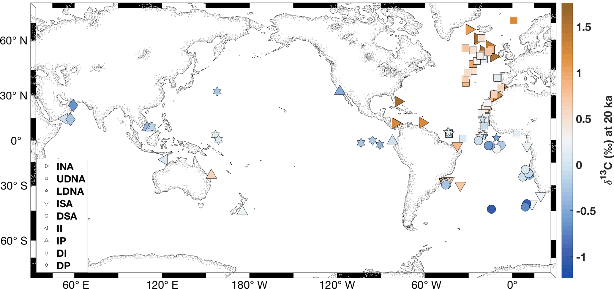
Figure 1Locations of 127 core sites compiled for this study, color coded by LGM δ13C estimates at each core site. Markers indicate locations of cores in the nine regions: INA is the intermediate North Atlantic; UDNA is the upper deep North Atlantic; LDNA is the lower deep North Atlantic; ISA is the intermediate South Atlantic; DSA is the deep South Atlantic; II is the intermediate Indian; DI is the deep Indian; IP is the intermediate Pacific; DP is the deep Pacific.
Multiple causes have been proposed for stronger vertical δ13C gradients during the LGM, including increased surface productivity and export, increased ocean stratification, and changes in preformed δ13C in regions of deep water formation (e.g., Matsumoto et al., 2002; Curry and Oppo, 2005; Marchitto and Broecker, 2006; Lynch-Stieglitz et al., 2007; Marinov et al., 2008a, b; Herguera et al., 2010; Hesse et al., 2011; Lund et al., 2011a, b; Allen et al., 2015; Gebbie et al., 2015; Schmittner and Somes, 2016; Gloege et al., 2017; Menviel et al., 2017). Therefore, the large vertical δ13C gradient at the LGM could indicate a strong biological pump and/or weak vertical mixing, either of which would increase deep ocean carbon storage. Although studies do not agree about the relative importance of different mechanisms in creating this vertical gradient, the consensus is that the enhanced vertical δ13C gradient at the LGM is consistent with greater deep ocean carbon storage and that this carbon was transferred to the atmosphere and terrestrial biosphere during the glacial termination. Multiple processes likely contribute to the deglacial pCO2 rise (Bauska et al., 2016), including ocean temperature increase, enhanced Southern Ocean mixing rates and the role of sea ice (e.g., Fraçnois et al., 1997; Crosta and Shemesh, 2002; Gildor et al., 2002; Hodell et al., 2003b; Paillard and Parrenin, 2004), decreased alkalinity and carbon inventories (Yu et al., 2014; Kerr et al., 2017), reduced biological pump (Buchanan et al., 2016), enhanced global ocean circulation (Buchanan et al., 2016), and coral reef growth (e.g., Vecsei and Berger, 2004).
On orbital timescales, changes in the intermediate-to-deep vertical δ13C gradient closely match atmospheric CO2, with weaker vertical δ13C gradients corresponding to higher CO2 levels (Oppo and Fairbanks, 1990; Flower et al., 2000; Hodell et al., 2003b; Köhler et al., 2010; Lisiecki, 2010). This relationship suggests that many of the processes affecting CO2 also alter the vertical δ13C gradient. Here we evaluate the relationship between atmospheric CO2 and vertical δ13C change at millennial resolution across the deglaciation. It is beyond the scope of this study to evaluate how much of the change in CO2 and the vertical δ13C gradient at the LGM is associated with specific processes, such as changes in the biological pump (Archer et al., 2003; Köhler et al., 2005; Brovkin et al., 2007; Galbraith and Jaccard, 2015), deep water formation (McManus et al., 2004; Curry and Oppo, 2005), and/or Southern Ocean stratification (Lund et al., 2011b; Burke and Robinson, 2012).
This study presents a compilation of 127 previously published benthic δ13C time series of Cibicides wuellerstorfi in per mil relative to Vienna PeeDee Belemnite (V.P.D.B.; Fig. 1; Table A1 in the Appendix). Each record in the compilation spans the time range 20–6 ka. Analysis does not extend after 6 ka because cores from several data-sparse regions were either of a too low resolution or missing sediment from 6–0 ka. We only include δ13C records with mean sample spacing better than 3 kyr, and 87 % have a mean sample spacing of less than 2 kyr. We excluded any records with sample gaps of 4 kyr or larger and excluded any cores affected by the phytodetritus effect (“Mackensen effect”) as assessed by the original authors and the criteria from Peterson et al. (2014). We included one C. kullenbergi record from the deep South Atlantic (MD07-3076Q; Waelbroeck et al., 2011), which may record a more negative δ13C value than C. wuellerstorfi at the LGM (Gottschalk et al., 2016). Additionally, we use some cores with samples labeled “C. spp” that may include some C. kullenbergi (Table A1).
4.1 Age models
For nearly all cores we use the age models of Stern and Lisiecki (2014) based on regional benthic δ18O alignments and seven regional age models. Each of the seven regions has an age model based on planktic 14C measurements from multiple cores; 14C dates are combined across cores by assuming that benthic δ18O is synchronous within each region (but not necessarily between regions). The first step of this process was generating an initial radiocarbon age model for each of the 61 cores by using that core's radiocarbon dates, the Bayesian age modeling software Bacon (Blaauw and Christen, 2011), the Marine13 calibration (Reimer et al., 2013), and constant 405 14C-yr reservoir ages. Bacon was used to estimate 14C-based ages at specified depths throughout each core, including Monte Carlo uncertainty estimates that increase with distance from the 14C measurements. To identify the core-specific depths for which 14C-based ages would be combined, each core's benthic δ18O record was aligned to an Atlantic or Pacific target core using the alignment software Match (Lisiecki and Lisiecki, 2002). Creating regional age models maximizes the total number of 14C dates which contribute to each age model. For example, the intermediate Pacific age model is derived from 14 sediment cores that include a total of 160 radiocarbon dates. The final age model for each core in Stern and Lisiecki (2014) was produced by converting from a (transitional) target age model based on benthic δ18O alignment to a regional composite radiocarbon age model.
Our compilation also includes δ13C records from 10 South Atlantic cores that were not included in Stern and Lisiecki (2014) and for which we used the core's published radiocarbon age models (Sortor and Lund, 2011; Hoffman and Lund, 2012; Tessin and Lund, 2013; Lund et al., 2015). These cores are denoted with asterisks in Table A1. The bulk of data compilation work for this study occurred in 2010–2015, and more recently published data are not included.
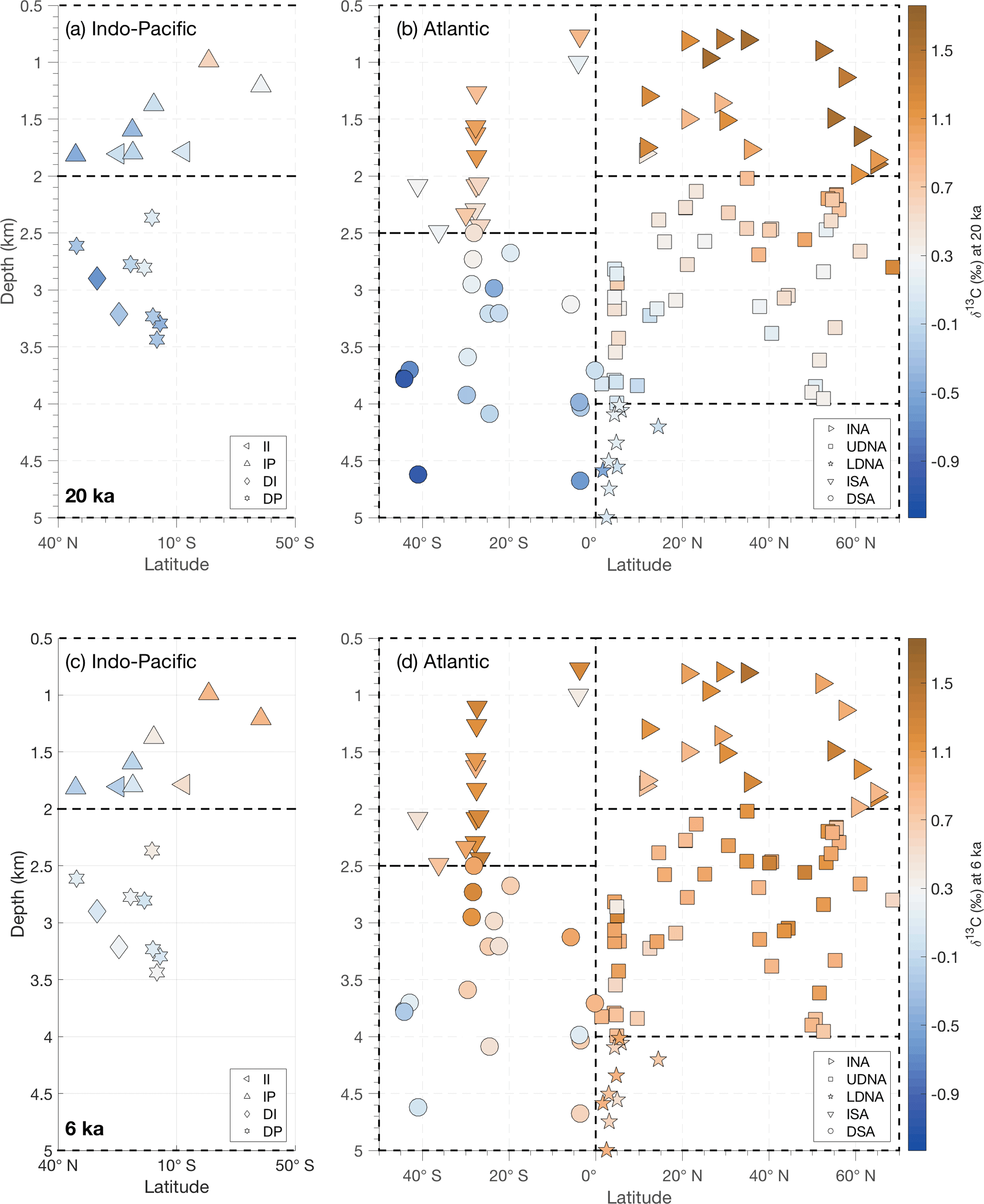
Figure 2The three-dimensional structure of δ13C in the Indian and Pacific oceans (a, c) and Atlantic (b, d) shown as zonally collapsed cross sections (latitude vs. modern water depth) with the same marker scheme as in Fig. 1. Dotted lines indicate region boundaries. Colors show the δ13C value at each site for the LGM (20 ka, a, b) and Holocene (6 ka, c, d). Note that latitudes on the x axis are oriented so the Southern Ocean is in the center of the figure. Additional time slices (in 1 kyr intervals from 20–6 ka) and an animation of deglacial δ13C changes can be found in the Supplement.
Table 1Regional stack information. The total volume represented by the global stack of all nine regions (spanning 0.5–5 km and excluding shallow inland seas, the Southern Ocean, and the Arctic Ocean) is 77.7 % of the whole ocean. The volume of each region is listed as a percent of the global stack volume (rather than whole ocean volume). For each stack we list its δ13C value at the LGM (20 ka), Holocene (6 ka), and the Holocene δ13C minus LGM δ13C difference. The 95 % confidence interval for the global mean δ13C change is provided in parentheses. The full time series for each stack is provided in the Supplement.
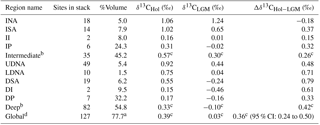
a Volume of all regions as a proportion of whole-ocean volume. b Atlantic and Pacific Ocean regions, excluding the Indian Ocean regions. c Volume-weighted δ13C values. d Atlantic, Indian, and Pacific Ocean regions.
Stern and Lisiecki (2014) estimate 95 % confidence intervals for each regional age model using 10 000 Monte Carlo age samples for each core from Bacon. Age uncertainty estimates for each region include the effects of any errors in benthic δ18O alignment because alignment errors would increase scatter in the compiled radiocarbon dates (by aligning portions of cores with different ages) and, thus, increase the observed spread in age estimates. For the time range of 6–20 kyr used in our δ13C compilation, the 95 % confidence interval widths of the regional age models range from 0.5–2.0 kyr. Although Match does not quantify alignment uncertainty, alignment uncertainties have been estimated using a similar algorithm, called HMM-Match (Lin et al., 2014). For age models generated either by δ18O alignment or radiocarbon dating, the amount of age uncertainty depends on the time resolution of the δ18O or 14C data, respectively. A comparison of 15 low-latitude Pacific cores found that 14C-based age uncertainty is comparable to, if not greater than, the uncertainty associated with δ18O alignments by HMM-Match (Khider et al., 2017).
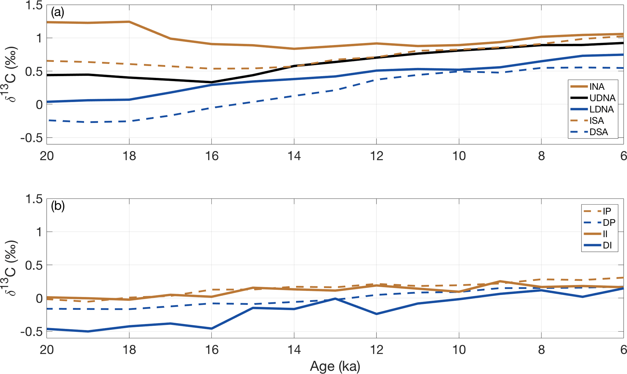
Figure 3Regional stacks for the (a) Atlantic and (b) Indian and Pacific oceans. Note the x and y axes are identically scaled. INA is the intermediate North Atlantic; UDNA is the upper deep North Atlantic; LDNA is the lower deep North Atlantic; ISA is the intermediate South Atlantic; DSA is the deep South Atlantic; II is the intermediate Indian; DI is the deep Indian; IP is the intermediate Pacific; DP is the deep Pacific.
4.2 Stacking
After compiling all 127 records of their previously published age models, we use spatial patterns in benthic δ13C to define nine ocean regions, for example, based on different LGM δ13C values for intermediate and deep sites (Fig. 2). In the North Atlantic, we separate the intermediate North Atlantic (INA, 0.5–2 km) from the upper deep North Atlantic (UDNA, 2–4 km) and the lower deep North Atlantic (LDNA, >4 km). Because the South Atlantic has fewer records than the North Atlantic (Table 1) and a different vertical δ13C structure (Fig. 2), we define the intermediate South Atlantic (ISA) as 0.5–2.5 km, and the deep South Atlantic (DSA) as >2.5 km. Although a zonal gradient is evident in the intermediate South Atlantic (Fig. 1), as also observed by Peterson et al. (2014), we combine all ISA records into a single region because only three sites are available in the east. We separate the Indo-Pacific into four regions: the intermediate Indian (II, 0.5–2 km), intermediate Pacific (IP, 0.5–2 km), deep Indian (DI, >2 km), and deep Pacific (DP, >2 km). The longitude boundaries between the Atlantic, Indian, and Pacific basins are the same as in Peterson et al. (2014). Most regions contain at least six sites; however, the intermediate and deep Indian regions each contain only two sites.
Although sea level rises globally by about 130–134 m (Lambeck et al., 2014; Clark et al., 2009) across the deglaciation, the volumetric change associated with deglacial sea level rise is small, less than 3 %. Therefore, we use modern water depths and volumes for all sites at all time steps. This preserves the spatial dimensions of the regions and prevents cores near region boundaries from switching between regions during the deglaciation.
To create regional stacks, we interpolated all benthic δ13C records to an even 1 kyr spacing and averaged all records within each region (Fig. 2; Table A1). The δ13C time series for sites KNR159-5-90GGC and KNR159-5-22GGC do not include 20 and 6 ka, respectively (Lund et al., 2015); at these times, the relevant sites were excluded from the regional average (Fig. 2 and the animation in the Supplement). Intermediate, deep, and global mean δ13C stacks (Figs. 3, 4) are calculated by averaging the regional stacks using volume weighting as a percent of total volume over a depth range of 0.5–5 km (Table 1). Thus, we represent regions proportional to their volume rather than over-representing well-sampled regions.

Figure 4Volume-weighted stacks. (a) The volume-weighted global stack is calculated based on all nine regional stacks. However, the intermediate and deep stacks shown here only include Atlantic and Pacific data due to the small amount of Indian data. A comparison of these stacks with ones which include the Indian stacks is provided in Fig. S1. (b) Stack uncertainty as characterized by the 95 % confidence interval half-width of each stack.
4.3 Stack limitations and uncertainty
Although our global stack includes benthic δ13C records from the Atlantic, Indian, and Pacific oceans, it does not include data from the Southern Ocean, Arctic Ocean, or shallow inland seas. Additionally, our compilation only includes benthic δ13C records from below 0.5 km. Although planktic δ13C data suggest that mixed layer δ13C values may closely track atmospheric δ13C change (Eggleston et al., 2016; Hertzberg et al., 2016), we refrain from interpreting or making assumptions about δ13C above 0.5 km. It is beyond the scope of the current study to quantify stack uncertainty associated with portions of the ocean which lack C. wuellerstorfi δ13C time series.
Uncertainty estimates for δ13C from C. wuellerstorfi range from 0.1 ‰ (Marchal and Curry, 2008) to 0.22 ‰ (experiments “LW” and “CW” in Schmittner et al., 2017). Accounting for the carbonate ion concentration of seawater can improve the accuracy of benthic δ13C (Schmittner et al., 2017), but estimates of carbonate ion changes throughout the deglaciation are scarce. In the absence of carbonate ion data, a linear regression can be used to convert between C. wuellerstorfi δ13C and DIC δ13C (regressions LW6 and CW6 in Schmittner et al., 2017). However, because our study focuses on the timing of δ13C change rather than its amplitude, we present all δ13C data using the values originally measured in foraminiferal calcite.
Interpolating the δ13C records to an even 1 kyr spacing introduces an additional source of uncertainty in the data. Although combining information from multiple records inherently risks distorting the true ocean state, this risk is counterbalanced by the potential for improved signal-to-noise ratio when estimating regional and global signals. In the Supplement, we provide the original, uninterpolated records for all 127 sites, which could be used for comparison with transient deglacial ocean circulation experiments. Because age model uncertainties are approximately 1–2 kyr (Stern and Lisiecki, 2014) and some of the δ13C records analyzed have sample spacings of 2–3 kyr, our interpretation focuses on δ13C features with timescales of about 2 kyr or greater. For example, we do not expect to reconstruct abrupt changes associated with the onset of the Bølling-Allerød or with centennial-scale CO2 change (Marcott et al., 2014).
We estimate stack uncertainty using Monte Carlo simulations that account for the effects of measurement uncertainty and intra-region δ13C variability. Specifically, we generate nominal 95 % confidence intervals for the stacks using 10 000 bootstrapped iterations that randomly resample δ13C records from each region. During the resampling process, we also simulate δ13C measurement uncertainty in each record by adding Gaussian white noise with a standard deviation of 0.20 ‰ (Gebbie et al., 2015). Multiple runs of our Monte Carlo simulations, each with 10 000 iterations, produce differences in the global benthic δ13C stack on the order of 0.02 ‰ at the LGM (20–19 ka) and less during the Holocene.
4.4 Comparison to atmospheric CO2
To compare the δ13C data to atmospheric CO2 changes from 20–6 ka, we calculate a vertical δ13C gradient (Δδ13CI−D) as the difference between the volume-weighted intermediate and deep regional stacks from the Atlantic and Pacific. The Indian Ocean regional stacks are excluded from this vertical gradient calculation because each Indian region includes only two sites, making the Indian regional stacks more susceptible to noise. A global vertical δ13C gradient that includes the Atlantic, Indian, and Pacific oceans (AIP Δδ13CI−D) is provided in the Supplement and in the Appendix (Fig. S1, Table A2). Additionally, we evaluate an alternate gradient, , defined as the difference between half the intermediate North Atlantic stack and the deep Pacific stack; Lisiecki (2010) found that this gradient optimized correlation with CO2 from 0–800 ka.
We interpolate a composite ice core CO2 record (Köhler et al., 2017) to the same 1 kyr resolution as our benthic δ13C stacks and calculate correlation coefficients between CO2 and the vertical gradient of δ13C. Additionally, we examine the potential for differences in the timing of CO2 and δ13C change that could be caused by lags in the climate system or age model uncertainty. We evaluate different potential lags by interpolating the CO2 record with different time offsets, ranging from +1000 to −1000 years in increments of 100 years. For example, a 100-year lag in CO2 relative to the vertical δ13C gradient would be represented by comparing δ13C values at 6, 7, …20 ka with CO2 values at 5.9, 6.9, …, and 19.9 ka. Conversely, a CO2 lead of 100 years would be suggested if the correlation between the two is maximized for CO2 values at 6.1, 7.1, …, 20.1 ka.
Testing the significance of correlations between δ13C and CO2 is complicated by the fact that both time series are autocorrelated, i.e., each data point is highly correlated with the value immediately before or after. To reduce the impact of autocorrelation, we pre-whiten the data by taking the difference between successive 1 kyr samples before calculating the linear correlation and its statistical significance. Our final assessment of the statistical significance of the correlations accounts for the reduction in the number of degrees of freedom in the data associated with pre-whitening and allowing time lags between δ13C and CO2 observations.
5.1 Comparison to LGM and Holocene reconstructions
Although our compilation of δ13C time series includes fewer core sites than some previous studies of LGM δ13C, it preserves the large-scale features of these glacial reconstructions, such as enhanced vertical and meridional Atlantic δ13C gradients (Fig. 2; e.g., Curry and Oppo, 2005; Peterson et al., 2014). Vertical δ13C gradients at the LGM are strongest in the glacial North Atlantic, closely followed by the glacial South Atlantic (Peterson et al., 2014). The most depleted δ13C values in the compilation are from the high-latitude deep South Atlantic during the LGM, possibly due to inclusion of data from C. kullenbergi (Gottschalk et al., 2016). Indo-Pacific δ13C values for the LGM are similar to equatorial deep South Atlantic records of the same depth and more depleted than North Atlantic δ13C values. However, our compilation lacks Indo-Pacific sites deeper than 3.5 km.
At 6 ka the δ13C values in this compilation generally resemble the Holocene compilation of Peterson et al. (2014). Minor differences could result from Peterson et al. (2014) using Holocene data from 6–0 ka and including more sites from the North Pacific sites and from 0.5–1.5 km depth.
5.2 Regional stacks
We create nine regional δ13C stacks from 20–6 ka (Fig. 3, Table 1). Six of the regional δ13C stacks increase steadily from approximately 20–18 to 6 ka (LDNA, DSA, II, IP, DI, DP). Small deviations in the trends of the Indian δ13C stacks are interpreted as noise because these stacks each contain only two δ13C records. Three Atlantic regions (INA, ISA, UDNA) show a decrease in δ13C from approximately 19–15 ka, followed by an increase from 14–6 ka, as described in previous studies (e.g., Hodell et al., 2008, 2010; Thornalley et al., 2010; Lund et al., 2011a; Tessin and Lund, 2013; Oppo et al., 2015). The UDNA δ13C stack has a δ13C value between the ISA and LDNA from 20–17 ka, approximately matches the LDNA at 16 ka, and then resembles the ISA stack from 14–6 ka. LDNA δ13C is slightly greater than DSA δ13C except at 10 ka when the two stacks briefly converge. The DI and DSA δ13C values are generally similar across the deglaciation except that the DSA δ13C begins increasing at 18 ka while the DI δ13C increase begins at 16 ka. The intermediate-depth δ13C stacks in the Indian and Pacific oceans are very similar for most of the time interval.
Across the deglaciation, the vertical δ13C gradient weakens in the Atlantic, most noticeably in the North Atlantic where the INA-LDNA gradient decreases from 1.20 ‰ at 20 ka to 0.31 ‰ at 6 ka. Vertical gradients in the Indian and Pacific oceans show much less change. The largest spread in δ13C values is observed from 20–18 ka, when the intermediate North Atlantic and deep South Atlantic regions differ by 1.50 ‰, a difference which decreases to 0.40 ‰ by 10 ka. The maximum difference between regions at 6 ka is 0.91 ‰ between the intermediate North Atlantic and the deep Indian.
5.3 Volume-weighted stacks and global mean δ13C stack
A global mean δ13C stack is constructed by volume weighting all nine regional stacks. However, we construct two versions of the intermediate and deep δ13C stacks, with and without the Indian stacks, because the Indian regions each contain only two records. Both versions of the intermediate and deep stacks show similar trends, but we focus our analysis on the version that uses only the Atlantic and Pacific regions, which should be less susceptible to noise (Fig. 4, Table 1). Results for the intermediate and deep δ13C stacks that include the Indian Ocean are provided in the Supplement and in the Appendix (Fig. S1, Table A2).
The volume-weighted intermediate, deep, and global mean δ13C stacks increase across the deglaciation, but the magnitude of change is larger for the deep stack (0.46 ‰) than the intermediate stack (0.24 ‰) (Table 1, Fig. 4). We define the vertical δ13C gradient, Δδ13CI−D, as the difference between the volume-weighted intermediate and deep stacks that exclude the data-sparse Indian regions. This gradient has a maximum of 0.41 ‰ at 18 ka and decreases to 0.24 ‰ by 6 ka.
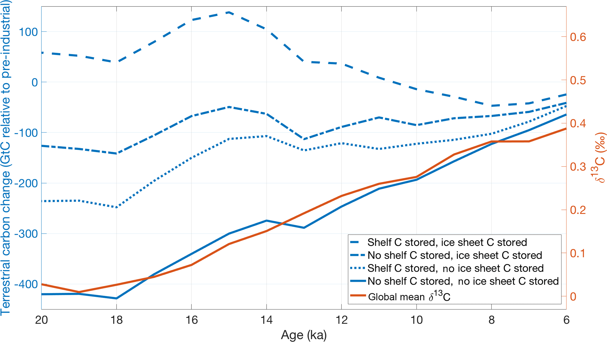
Figure 5Four HadCM3 simulations of terrestrial carbon storage change (biosphere and soils) to the pre-industrial (blue, Davies-Barnard et al., 2017) compared to our volume-weighted global benthic δ13C stack (orange). Global mean δ13C change most closely resembles the simulation that releases carbon from under ice sheets to the atmosphere and does not store carbon on continental shelves (solid blue). The two y axes are scaled to illustrate the similarity in the pattern of change across the deglaciation but are not meant to imply that the magnitude of change is equivalent.
The volume-weighted global δ13C stack holds nearly steady from 20 to 19 ka at approximately 0.00 ‰ (95 % CI: −0.13 to 0.12 ‰ at 19 ka) and then increases from 18–6 ka, reaching a value of 0.39 ‰ (95 % CI: 0.24 to 0.49 ‰) at 6 ka. The change from 20 to 6 ka in the global stack is 0.36 ‰ (95 % CI: 0.24 to 0.50 ‰), which agrees to within uncertainty with the LGM-to-Holocene δ13C change of 0.38 ‰ (95 % CI: 0.30 to 0.46 ‰) estimated for 0.5–5 km by Peterson et al. (2014). Recall that the mean δ13C estimate from our global stack is not quite a whole-ocean δ13C estimate because we do not include data from the surface (<0.5 km), Southern Ocean (>65∘ S), or bottom waters (>5 km). Estimates of whole-ocean δ13C change are slightly smaller at 0.34 ‰ (95 % CI: 0.15 to 0.53 ‰; Peterson et al., 2014) and 0.32 ‰ (95 % CI: 0.12 to 0.52 ‰; Gebbie et al., 2015) because the surface ocean (0–0.5 km) has less deglacial change (Eggleston et al., 2016; Hertzberg et al., 2016).
6.1 Terrestrial carbon storage and global mean benthic δ13C
The long-standing explanation for mean benthic δ13C change across the deglaciation is an increase in the size of the terrestrial biosphere (Shackleton, 1977; Curry et al., 1988; Duplessy et al., 1988). Here we compare the timing of changes in our global mean δ13C stack (i.e., a monotonic increase from 19–6 ka, Fig. 4b) with model simulations and other terrestrial biosphere reconstructions.
A carbon isotope-enabled transient model from Lund-Potsdam-Jena Dynamic Global Vegetation Model (LPJ-DGVM) simulated a mean ocean δ13C increase beginning at 21 ka, with the most rapid changes occurring from 17–10.5 ka (Kaplan et al., 2002). In these experiments, the terrestrial biosphere began expanding around 18–16.5 ka (Joos et al., 2004; Köhler et al., 2005) and rapidly increased from 17–9 ka, with 70 % of terrestrial carbon storage change occurring before the Holocene (11.5 ka; Kaplan et al., 2002). Similarly, 67 % of the change in our global δ13C stack occurs between 19–11 ka while the remaining 33 % occurs from 11–6 ka.
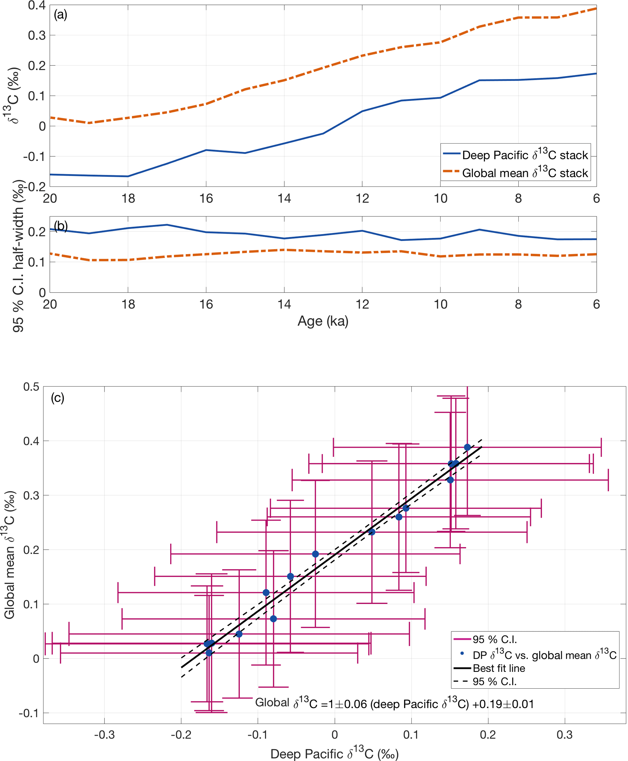
Figure 6(a) Time series of global mean ocean δ13C stack and deep Pacific δ13C stacks. (b) Half-width 95 % confidence intervals for the global mean stack and deep Pacific stack. (c) Deep Pacific δ13C stack vs. global mean δ13C stack. Each point is the δ13C value for one time slice with 95 % confidence intervals (vertical and horizontal error bars). Time across the deglaciation progresses toward the upper right corner. The best-fit linear regression is plotted as a solid line with 95 % confidence interval (dashed lines).
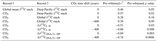
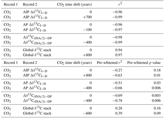
Table 2Correlation coefficients and p values between pre-whitened records. Pre-whitening reduces the impact of autocorrelation in the time series. Calculated p values account for the reduced degrees of freedom in pre-whitened and time-lagged correlations. Non-zero CO2 time shifts indicate the lead/lag adjustment that maximizes the correlation between atmospheric CO2 Köhler et al. (2017) and the δ13C stack or gradient.
Simulations from HadCM3 estimated that 45 %–70 % of terrestrial biosphere expansion occurred between 18–14 ka (Davies-Barnard et al., 2017). Dramatically different trends were observed from 14–6 ka in simulations with different assumptions about carbon storage under glacial ice sheets and on continental shelves. The simulation that most closely resembles our global mean δ13C stack is the simulation that releases carbon from under ice sheets to the atmosphere and does not accumulate carbon on exposed continental shelves (Fig. 5). This simulation is also the only one which agrees with terrestrial carbon storage change estimates of 440 PgC based on whole-ocean mean δ13C change (e.g., Peterson et al., 2014).
Holocene simulations using a global pollen synthesis, the biomization method, and models of climate and vegetation (HadCM3, FAMOUS, and BIOME4) suggest that the global average area for most carbon-rich megabiomes (i.e., excluding grasslands and dry shrubland) increased from 10–2 ka and net primary productivity increased from 8–2 ka (Hoogakker et al., 2016). This is consistent with our observation that the global mean benthic δ13C trend continued until at least 6 ka. Dramatic land use changes from agricultural practices, another potential mechanism for terrestrial carbon change, did not begin until 4.5 ka (Ruddiman and Ellis, 2009). More detailed evaluation of Holocene terrestrial carbon storage changes will require improved spatial coverage for δ13C records from 6–0 ka.
6.2 Deep Pacific and global mean δ13C
Previous studies have assumed deep Pacific δ13C can be used as a proxy for global mean δ13C because the deep Pacific constitutes about 30 % of the ocean volume and is not strongly affected by shifting water mass boundaries (e.g., Shackleton et al., 1983; Curry and Oppo, 1997; Lisiecki et al., 2008). From 20–6 ka, the global mean and deep Pacific δ13C stacks show similar patterns of change (Fig. 6) and fall along a tight regression line
The two time series are highly correlated (r2=0.99), which is not surprising because the large volume of the deep Pacific exerts a strong influence on the global mean δ13C stack. When the stacks are pre-whitened to account for autocorrelation (Table 2), their correlation is weaker (r2=0.46) but statistically significant (p=0.05).
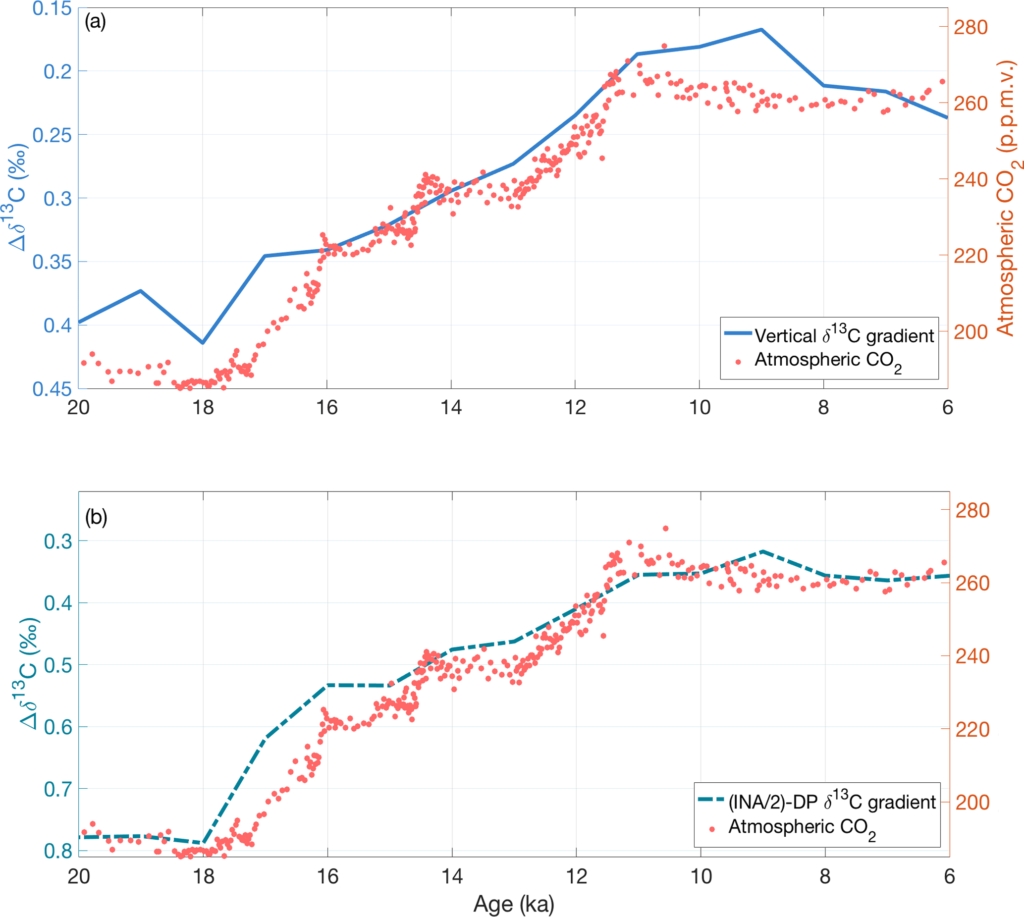
Figure 7Comparison of atmospheric CO2 with (a) the vertical δ13C gradient (excluding the data-sparse Indian Ocean regions) and (b) . Both gradients have a statistically significant correlation with atmospheric CO2 records (red circles, Köhler et al., 2017). The y axes for (a) and (b) are scaled differently because scales the intermediate North Atlantic stack by half before subtracting the deep Pacific stack while the δ13C gradient is the difference between the intermediate and deep stacks (Atlantic and Pacific oceans only).
Alternatively, a carbon cycle box model simulated a strong correlation between deep Pacific δ13C and CO2 across several glacial cycles (r2=0.96; Köhler et al., 2010). The correlation between CO2 and our deep Pacific δ13C stack is statistically significant after pre-whitening (r2=0.57, p=0.02), but global mean δ13C and CO2 are not (r2=0.28, p=0.16). Our compilation of Pacific records is likely insufficient to determine whether deep Pacific δ13C correlates better with global mean δ13C or atmospheric CO2. This issue could be better resolved using a δ13C compilation spanning multiple glacial cycles and including more deep Pacific sites.
6.3 Vertical δ13C gradient and atmospheric CO2
The vertical δ13C gradient (Δδ13CI−D) in our compilation resembles the inverse of CO2 change across the deglaciation (Fig. 7), as would be expected if they are both strongly influenced by changes in deep ocean carbon storage (Flower et al., 2000; Oppo and Horowitz, 2000; Hodell et al., 2003b). Alternatively, one orbital-scale study found a stronger correlation with CO2 using the gradient between the deep Pacific and half the INA δ13C stack (), Lisiecki (2010). Both vertical δ13C gradients (Δδ13CI−D and ) decrease from 18–11 ka over the same time interval that atmospheric CO2 increases. In contrast, the global mean δ13C stack increases at a relatively steady pace from 19–6 ka. Thus, the δ13C gradients record a distinctly different signal than global mean δ13C.
The δ13C gradients decrease most rapidly across two time steps, 18–17 and 12–11 ka. The first change at 18 ka is approximately synchronous with the start of atmospheric CO2 rise (Marcott et al., 2014; Köhler et al., 2017) and a decrease of 0.3 ‰ in the δ13C of atmospheric CO2 (Eggleston et al., 2016). In the Southern Ocean at 18 ka, proxy records indicate a decrease in aeolian dust deposition accompanied by lower marine productivity (Martínez-Garcia et al., 2009) and a decrease in winter sea ice cover, which likely reduced vertical stratification (Ferrari et al., 2014). The second rapid change in the vertical δ13C gradients at 12 ka approximately coincides with rapidly increasing atmospheric CO2 from 13–11.5 ka and a decrease of 0.1 ‰ in the δ13C of atmospheric CO2.
From 11 to 6 ka, atmospheric CO2 remains nearly constant with a small (approximately 10 ppm) decrease from 11–8 ka. The vertical δ13C gradients are also relatively steady from 11–6 ka, with a slight increase in both gradients from 9–8 ka. The small decrease in atmospheric CO2 beginning at 11 ka (Marcott et al., 2014) has been variously attributed to growth of the terrestrial biosphere, sea level rise, and an increase in gas exchange through reduced sea ice cover (Kaplan et al., 2002; Joos et al., 2004; Köhler and Fischer, 2004; Köhler et al., 2005, 2010).
Although CO2 correlates strongly with both Δδ13CI−D () and (), we must pre-whiten these time series to remove autocorrelation before assessing the statistical significance of their correlation. At the 95 % confidence level, atmospheric CO2 significantly correlates with both Δδ13CI−D (; p=0.03) and (; p<0.01) (Fig. S1, Table 2). Better correlation with could be because of better age control and higher resolution δ13C records in the INA region than the other intermediate regions. Determining whether the gradient or the global vertical δ13C gradient correlates better with atmospheric CO2 will require data with better spatial coverage and/or a longer time span.
Because our comparison of the vertical δ13C gradient and CO2 could be affected by lags within the carbon cycle or age model uncertainty, we additionally investigate whether the correlations between CO2 and the vertical δ13C gradient would be improved by age model shifts (Table 2). The correlation between CO2 is maximized when Δδ13CI−D or lags CO2 by 400 years (Table 2), which is within the age uncertainty of the sediment core age models. Thus, changes in atmospheric CO2 and vertical δ13C gradients appear synchronous to within age model uncertainty.
Processes that potentially explain atmospheric CO2 change during glacial cycles include the efficiency of the biological pump (Martínez-Garcia et al., 2009; Galbraith and Jaccard, 2015), circulation changes (Ferrari et al., 2014; Schmittner and Lund, 2015; Lacerra et al., 2017; Menviel et al., 2017; Sikes et al., 2017; Wagner and Hendy, 2017), or a combination of multiple processes (Bauska et al., 2016; Skinner et al., 2017). Different processes could influence the carbon cycle on different timescales (Bauska et al., 2016; Kohfeld and Chase, 2017) and/or in different regions (e.g., Gu et al., 2017) and complicate interpretations of which processes are most responsible for atmospheric CO2 change. However, because both productivity and circulation change would affect the vertical δ13C gradient while changing atmospheric CO2, we interpret our results as supporting the importance of the deep ocean as a reservoir for storing glacial carbon related to either or both processes. Furthermore, these results support the use of vertical δ13C gradients as a proxy for glacial–interglacial CO2 change on both orbital and millennial timescales (Lisiecki, 2010).
We present regional δ13C stacks and volume-weighted intermediate, deep, and global mean δ13C stacks from a compilation of 127 benthic C. wuellerstorfi δ13C records, which span 20 to 6 kyr with a mean age resolution better than 2 kyr. Age models are based on δ18O alignments to regional stacks with radiocarbon dating and age model uncertainties of approximately 1–2 kyr. Our compilation shows spatial patterns in benthic δ13C that are similar to higher resolution reconstructions of the Holocene and Last Glacial Maximum. The volume-weighted mean δ13C change estimated from these 127 records is 0.36 ‰ (95 % CI: 0.24 to 0.50 ‰), similar to the estimate of Peterson et al. (2014) for 0.5–5 km based on 480 records.
Importantly, this global compilation of benthic δ13C time series also allows us to evaluate the timing of change in the mean and vertical gradient of δ13C and compare them with other carbon cycle changes. The volume-weighted global δ13C stack increases from 19 to 6 ka and likely reflects terrestrial biosphere growth, in agreement with model simulations (Kaplan et al., 2002; Joos et al., 2004; Davies-Barnard et al., 2017). To constrain the timing of the end of terrestrial biosphere expansion, future work should focus on extending the global stack through the Late Holocene. Furthermore, δ13C changes from 20 to 6 ka suggest that a deep Pacific δ13C stack approximates global mean δ13C with an offset of 0.19 ‰. Vertical δ13C gradients between intermediate and deep water (Δδ13CI−D) and between the intermediate North Atlantic and deep Pacific () are interpreted as proxies for change in deep ocean carbon storage. Millennial-scale features in Δδ13CI−D and are significantly correlated with atmospheric CO2 changes from 20–6 ka.
Based on these analyses, we conclude that the four-dimensional compilation of globally distributed δ13C time series presented here provides useful constraints for global carbon cycle reconstructions and for comparison with deglacial simulations from isotope-enabled Earth system models.
The original data and publication citations along with this data synthesis are made available in the Supplement and at PANGAEA.
Table A1Supplemental table of the name, location, region, and reference for each record in this δ13C synthesis. Asterisks mark cores for which we use the cited authors' radiocarbon age model instead of using the regional age model from Stern and Lisiecki (2014). Data repository links for each δ13C record are provided in Table S1 in the Supplement.

Table A2Correlation coefficients and p values between records. The upper rows use the raw data, and the bottom rows use pre-whitened data to account for autocorrelated time series. AIP gradients include Atlantic, Indian, and Pacific regions, and AP gradients include only Atlantic and Pacific regions. To investigate possible leads/lags between records, we shift the atmospheric CO2 record in 100-year increments relative to the δ13C stacks and, for brevity, list only the best correlations. All p values account for reduction in degrees of freedom due to pre-whitening and/or time shifting.
The supplement related to this article is available online at: https://doi.org/10.5194/cp-14-1229-2018-supplement.
LEL contributed to the design of the experiment, interpretation of results, and manuscript revision. CDP contributed data collection, performed the analysis, interpreted results, and wrote the manuscript.
The authors declare that they have no conflict of interest.
This article is part of the special issue “Paleoclimate data synthesis and analysis of associated uncertainty (BG/CP/ESSD inter-journal SI)”. It is not associated with a conference.
We acknowledge the following colleagues and reviewers whose advice and input
substantially improved drafts of this manuscript: David Lea, Syee Weldeab,
Jake Gebbie, Andy Ridgwell, James Rae, Andreas Schmittner, Peter Köhler,
Lukas Jonkers, and an anonymous reviewer. Additionally, we thank the staff at
PANGAEA, Delphi, and NOAA-NCDC data repositories who helped verify details of
data sets, DOIs, URLs, and references. Funding for this work came from NSF grants MGG 0926735 and CDI
1125181.
Edited by: Lukas
Jonkers
Reviewed by: Andreas Schmittner and one anonymous
referee
Allen, K. A., Sikes, E. L., Hönisch, B., Elmore, A. C., Guilderson, T. P., Rosenthal, Y., and Anderson, R. F.: Southwest Pacific deep water carbonate chemistry linked to high southern latitude climate and atmospheric CO2 during the last glacial termination, Quaternary Sci. Rev., 122, 180–191, 2015. a, b
Archer, D., Winguth, A., Lea, D., and Mahowald, N.: What caused the glacial/interglacial atmospheric pCO2 cycles?, Rev. Geophys., 38, 159–190, 2000. a
Archer, D. E., Martin, P. A., Milovich, J., Brovkin, V., Plattner, G.-K., and Ashendel, C.: Model sensitivity in the effect of Antarctic sea ice and stratification on atmospheric pCO2, Paleoceanography, 18, 1012, https://doi.org/10.1029/2002PA000760, 2003. a
Arz, H. W., Pätzold, J., and Wefer, G.: Stable oxygen and carbon isotope ratios of benthic foraminifera from sediment core GeoB3104-1, PANGAEA, https://doi.org/10.1594/PANGAEA.54790, 1999. a
Aydin, M., Campbell, J., Fudge, T., Cuffey, K., Nicewonger, M., Verhulst, K., and Saltzman, E.: Changes in atmospheric carbonyl sulfide over the last 54,000 years inferred from measurements in Antarctic ice cores, J. Geophys. Res.-Atmos., 121, 1943–1954, https://doi.org/10.1002/2015JD024235, 2016. a
Bauska, T. K., Baggenstos, D., Brook, E. J., Mix, A. C., Marcott, S. A., Petrenko, V. V., Schaefer, H., Severinghaus, J. P., and Lee, J. E.: Carbon isotopes characterize rapid changes in atmospheric carbon dioxide during the last deglaciation, P. Natl. Acad. Sci. USA, 113, 3465–3470, 2016. a, b, c
Bickert, T., Wefer, G., and Müller, P. J.: Stable isotopes and sedimentology of core GeoB1117-2, PANGAEA, https://doi.org/10.1594/PANGAEA.58780, 2001. a
Bickert, T., Wefer, G., and Müller, P. J.: Stable isotopes and sedimentology of core GeoB1101-4, PANGAEA, https://doi.org/10.1594/PANGAEA.103621, 2003a. a
Bickert, T., Wefer, G., and Müller, P. J.: Stable isotopes and sedimentology of core GeoB1112-3, PANGAEA, https://doi.org/10.1594/PANGAEA.103625, 2003b. a
Bickert, T., Wefer, G., and Müller, P. J.: Stable isotopes and sedimentology of core GeoB1214-1, PANGAEA, https://doi.org/10.1594/PANGAEA.103635, 2003c. a
Bickert, T., Wefer, G., and Müller, P. J.: Stable isotopes and sedimentology of core GeoB1041, PANGAEA, https://doi.org/10.1594/PANGAEA.58771, 2009a. a, b
Bickert, T., Wefer, G., and Müller, P. J.: Stable isotopes and sedimentology of core GeoB1211, PANGAEA, https://doi.org/10.1594/PANGAEA.58782, 2009b. a
Blaauw, M. and Christen, J. A.: Flexible paleoclimate age-depth models using an autoregressive gamma process, Bayesian Anal., 6, 457–474, 2011. a
Bostock, H. C., Opdyke, B. N., Gagan, M. K., and Fifield, L. K.: Stable isotopes from sediment core FR01/97-12, Tasman Sea, PANGAEA, https://doi.org/10.1594/PANGAEA.832096, 2004. a
Boyle, E. A.: Cadmium and δ13C paleochemical ocean distributions during the stage 2 Glacial Maximum, Annu. Rev. Earth Pl. Sc., 20, 245–287, 1992. a
Broecker, W. S.: Ocean chemistry during glacial time, Geochim. Cosmochim. Ac., 46, 1689–1705, 1982. a
Brovkin, V., Ganopolski, A., Archer, D., and Rahmstorf, S.: Lowering of glacial atmospheric CO2 in response to changes in oceanic circulation and marine biogeochemistry, Paleoceanography, 22, PA4202, https://doi.org/10.1029/2006PA001380, 2007. a, b
Brovkin, V., Ganopolski, A., Archer, D., and Munhoven, G.: Glacial CO2 cycle as a succession of key physical and biogeochemical processes, Clim. Past, 8, 251–264, https://doi.org/10.5194/cp-8-251-2012, 2012. a
Buchanan, P. J., Matear, R. J., Lenton, A., Phipps, S. J., Chase, Z., and Etheridge, D. M.: The simulated climate of the Last Glacial Maximum and insights into the global marine carbon cycle, Clim. Past, 12, 2271–2295, https://doi.org/10.5194/cp-12-2271-2016, 2016. a, b, c
Burke, A. and Robinson, L. F.: The Southern Ocean's role in carbon exchange during the last deglaciation, Science, 335, 557–561, 2012. a
Chen, M.-T.: Carbon and oxygen isotopes from benthic foraminifera of sediment core MD97-2151, PANGAEA, available at: https://doi.pangaea.de/10.1594/PANGAEA.114672, 2003. a
Ciais, P., Tagliabue, A., Cuntz, M., Bopp, L., Scholze, M., Hoffmann, G., Lourantou, A., Harrison, S. P., Prentice, I., Kelley, D., and Koven, C.: Large inert carbon pool in the terrestrial biosphere during the Last Glacial Maximum, Nat. Geosci., 5, 74–79, 2012. a
Clark, P. U., Dyke, A. S., Shakun, J. D., Carlson, A. E., Clark, J., Wohlfarth, B., Mitrovica, J. X., Hostetler, S. W., and McCabe, A. M.: The last glacial maximum, Science, 325, 710–714, 2009. a
Cortijo, E., Scott, L., Keigwin, L. D., Chapman, M. R., Paillard, D., and Labeyrie, L. D.: (Fig. 3a) Stable oxygen isotope ratios of benthic foraminifera of sediment core SU90-03, PANGAEA, https://doi.org/10.1594/PANGAEA.857320, 1999. a
Crosta, X. and Shemesh, A.: Reconciling down core anticorrelation of diatom carbon and nitrogen isotopic ratios from the Southern Ocean, Paleoceanography, 17, 10-1–10-8, https://doi.org/10.1029/2000PA000565, 2002. a
Curry, W. B.: Stable isotope analysis on sediment core RC13-228, PANGAEA, https://doi.org/10.1594/PANGAEA.139596, 2004. a
Curry, W. B. and Lohmann, G.: Carbon isotopic changes in benthic foraminifera from the western South Atlantic: Reconstruction of glacial abyssal circulation patterns, Quaternary Res., 18, 218–235, 1982a. a
Curry, W. B. and Lohmann, G. P.: Stable carbon and oxygen isotope ratios of Planulina wuellerstorfi from sediments of the Vema Channel, PANGAEA, https://doi.org/10.1594/PANGAEA.726254, 1982b. a
Curry, W. B. and Lohmann, G. P.: (Table 1) Stable carbon and oxygen isotope ratios of Planulina wuellerstorfi from sediment core EN066-38PG, PANGAEA, https://doi.org/10.1594/PANGAEA.726019, 1983a. a
Curry, W. B. and Lohmann, G. P.: (Table 1) Stable carbon and oxygen isotope ratios of Planulina wuellerstorfi from sediment core EN066-16PG, PANGAEA, https://doi.org/10.1594/PANGAEA.726013, 1983b. a
Curry, W. B. and Lohmann, G. P.: (Table 1) Stable carbon and oxygen isotope ratios of Planulina wuellerstorfi from sediment core EN066-21PG, PANGAEA, https://doi.org/10.1594/PANGAEA.726014, 1983c. a
Curry, W. B. and Lohmann, G. P.: (Table 1) Stable carbon and oxygen isotope ratios of Planulina wuellerstorfi from sediment core EN066-26PG, PANGAEA, https://doi.org/10.1594/PANGAEA.726015, 1983d. a
Curry, W. B. and Lohmann, G. P.: (Table 1) Stable carbon and oxygen isotope ratios of Planulina wuellerstorfi from sediment core EN066-36PG, PANGAEA, https://doi.org/10.1594/PANGAEA.726018, 1983e. a
Curry, W. B. and Lohmann, G. P.: (Table 1) Stable carbon and oxygen isotope ratios of Planulina wuellerstorfi from sediment core EN066-44PG, PANGAEA, https://doi.org/10.1594/PANGAEA.726020, 1983f. a
Curry, W. B. and Lohmann, G. P.: (Table 1) Stable carbon and oxygen isotope ratios of Planulina wuellerstorfi from sediment core EN066-32PG, PANGAEA, https://doi.org/10.1594/PANGAEA.726017, 1983g. a
Curry, W. B. and Oppo, D. W.: Stable isotope record of foraminifera from sediment core EW9209-1JPC, PANGAEA, https://doi.org/10.1594/PANGAEA.730044, 1997. a
Curry, W. B. and Oppo, D. W.: Synchronous, high-frequency oscillations in tropical sea surface temperatures and North Atlantic Deep Water production during the last glacial cycle, Paleoceanography, 12, 1–14, 1997. a, b, c
Curry, W. B. and Oppo, D. W.: Glacial water mass geometry and the distribution of δ13C of ΣCO2 in the western Atlantic Ocean, Paleoceanography, 20, PA1017, https://doi.org/10.1029/2004PA001021, 2005 (data available at: https://www.ncdc.noaa.gov/paleo/study/8673, last access: 8 August 2018). a, b, c, d, e, f, g
Curry, W. B., Duplessy, J.-C., Labeyrie, L., and Shackleton, N. J.: Changes in the distribution of δ13C of deep water ΣCO2 between the last glaciation and the Holocene, Paleoceanography, 3, 317–341, 1988. a, b, c, d, e
Curry, W. B., Duplessy, J.-C., Labeyrie, L. D., and Shackleton, N. J.: (Appendix 1) Stable carbon and oxygen isotope ratios of Cibicidoides spp. from sediment core BT4, PANGAEA, https://doi.org/10.1594/PANGAEA.52328, 1988a. a
Curry, W. B., Duplessy, J.-C., Labeyrie, L. D., and Shackleton, N. J.: (Appendix 1) Stable carbon and oxygen isotope ratios of Cibicidoides spp. from sediment core CHN82-24, PANGAEA, https://doi.org/10.1594/PANGAEA.52327, 1988b. a
Curry, W. B., Duplessy, J.-C., Labeyrie, L. D., and Shackleton, N. J.: (Appendix 1) Stable carbon and oxygen isotope ratios of Cibicidoides wuellerstorfi from sediment core KNR110-0082GGC, PANGAEA, https://doi.org/10.1594/PANGAEA.357162, 1988c. a, b
Curry, W. B., Duplessy, J.-C., Labeyrie, L. D., and Shackleton, N. J.: (Appendix 1) Stable carbon and oxygen isotope ratios of Cibicidoides wuellerstorfi from sediment core KNR110-0050GGC, PANGAEA, https://doi.org/10.1594/PANGAEA.357156, 1988d. a
Curry, W. B., Duplessy, J.-C., Labeyrie, L. D., and Shackleton, N. J.: (Appendix 1) Stable carbon and oxygen isotope ratios of Cibicidoides wuellerstorfi from sediment core KNR110-0055GGC, PANGAEA, https://doi.org/10.1594/PANGAEA.357157, 1988e. a
Curry, W. B., Duplessy, J.-C., Labeyrie, L. D., and Shackleton, N. J.: (Appendix 1) Stable carbon and oxygen isotope ratios of Cibicidoides wuellerstorfi from sediment core KNR110-0058GGC, PANGAEA, https://doi.org/10.1594/PANGAEA.357158, 1988f. a
Curry, W. B., Duplessy, J.-C., Labeyrie, L. D., and Shackleton, N. J.: (Appendix 1) Stable carbon and oxygen isotope ratios of Cibicidoides wuellerstorfi from sediment core KNR110-0066GGC, PANGAEA, https://doi.org/10.1594/PANGAEA.357159, 1988g. a
Curry, W. B., Duplessy, J.-C., Labeyrie, L. D., and Shackleton, N. J.: (Appendix 1) Stable carbon and oxygen isotope ratios of Cibicidoides wuellerstorfi from sediment core KNR110-0071GGC, PANGAEA, https://doi.org/10.1594/PANGAEA.357160, 1988h. a
Curry, W. B., Duplessy, J.-C., Labeyrie, L. D., and Shackleton, N. J.: (Appendix 1) Stable carbon and oxygen isotope ratios of Cibicidoides wuellerstorfi from sediment core KNR110-0091GGC, PANGAEA, https://doi.org/10.1594/PANGAEA.357163, 1988i. a
Curry, W. B., Duplessy, J.-C., Labeyrie, L. D., and Shackleton, N. J.: Stable carbon and oxygen isotope ratios of benthic foraminifera, PANGAEA, https://doi.org/10.1594/PANGAEA.726195, 1988j. a
Curry, W. B., Duplessy, J.-C., Labeyrie, L. D., and Shackleton, N. J.: (Appendix 1) Stable carbon and oxygen isotope ratios of Cibicidoides spp. from sediment core V22-197, PANGAEA, https://doi.org/10.1594/PANGAEA.52291, 1988k. a
Curry, W. B., Duplessy, J.-C., Labeyrie, L. D., and Shackleton, N. J.: (Appendix 1) Stable carbon and oxygen isotope ratios of Cibicidoides wuellerstorfi from sediment core V25-59, PANGAEA, https://doi.org/10.1594/PANGAEA.52290, 1988l. a
Curry, W. B., Duplessy, J.-C., Labeyrie, L. D., and Shackleton, N. J.: (Appendix 1) Stable carbon and oxygen isotope ratios of Cibicidoides wuellerstorfi from sediment core V30-49, PANGAEA, https://doi.org/10.1594/PANGAEA.52280, 1988m. a
Curry, W. B., Marchitto, T. M., McManus, J. F., Oppo, D. W., and Laarkamp, K. L.: Millennial-scale changes ventilation of the thermocline, intermediate and deep waters of the Glacial North Atlantic, Geophysical Monograph, 112, 59–76, https://doi.org/10.1029/GM112p0059, 1999 (data available at: ftp://ftp.ncdc.noaa.gov/pub/data/paleo/contributions_by_author/curry1999/cibs_103ggc_all_calendar.txt, last access: 13 August 2018). a
Davies-Barnard, T., Ridgwell, A., Singarayer, J., and Valdes, P.: Quantifying the influence of the terrestrial biosphere on glacial–interglacial climate dynamics, Clim. Past, 13, 1381–1401, https://doi.org/10.5194/cp-13-1381-2017, 2017. a, b, c, d
Demenocal, P. B., Oppo, D. W., Fairbanks, R. G., and Prell, W. L.: Pleistocene δ13C variability of North Atlantic intermediate water, Paleoceanography, 7, 229–250, https://doi.org/10.1029/92PA00420, 1992 (data available at: https://www.ncdc.noaa.gov/paleo-search/study/2554, last access: 7 August 2018). a
Dorschel, B., Hebbeln, D., Rüggeberg, A., Dullo, W. C., and Freiwald, A.: (Appendix 3) Stable isotopes of sediment core GeoB6718-2, PANGAEA, https://doi.org/10.1594/PANGAEA.134554, 2005. a
Duplessy, J., Shackleton, N., Fairbanks, R., Labeyrie, L., Oppo, D., and Kallel, N.: Deepwater source variations during the last climatic cycle and their impact on the global deepwater circulation, Paleoceanography, 3, 343–360, 1988. a, b, c, d, e, f
Duplessy, J.-C.: (Table 6) Stable carbon and oxygen isotope ratios of Cibicides species from sediment core CH73-139, PANGAEA, https://doi.org/10.1594/PANGAEA.726215, 1982. a
Duplessy, J.-C.: Stable isotope of sediment core NA87-22, PANGAEA, https://doi.org/10.1594/PANGAEA.54411, 1997. a
Eggleston, S., Schmitt, J., Bereiter, B., Schneider, R., and Fischer, H.: Evolution of the stable carbon isotope composition of atmospheric CO2 over the last glacial cycle, Paleoceanography, 31, 434–452, https://doi.org/10.1002/2015PA002874, 2016. a, b, c, d, e
Ferrari, R., Jansen, M. F., Adkins, J. F., Burke, A., Stewart, A. L., and Thompson, A. F.: Antarctic sea ice control on ocean circulation in present and glacial climates, P. Natl. Acad. Sci. USA, 111, 8753–8758, 2014. a, b
Flower, B. P., Oppo, D. W., McManus, J., Venz, K., Hodell, D., and Cullen, J.: North Atlantic intermediate to deep water circulation and chemical stratification during the past 1 Myr, Paleoceanography, 15, 388–403, https://doi.org/10.1029/1999PA000430, 2000. a, b, c, d
Fraçnois, R., Altabet, M. A., Yu, E.-F., Sigman, D. M., Bacon, M. P., Frank, M., Bohrmann, G., Bareille, G., and Labeyrie, L. D.: Contribution of Southern Ocean surface-water stratification to low atmospheric CO2 concentrations during the last glacial period, Nature, 389, 929–935, 1997. a
Freudenthal, T., Meggers, H., Henderiks, J., Kuhlmann, H., Moreno, A., and Wefer, G.: Age model, stable isotope record, CaCO3 and TOC of sediment core GeoB4240-2, PANGAEA, https://doi.org/10.1594/PANGAEA.57859, 2002a. a
Freudenthal, T., Meggers, H., Henderiks, J., Kuhlmann, H., Moreno, A., and Wefer, G.: Age model, stable isotope record, CaCO3 and TOC of sediment core GeoB4216-1, PANGAEA, https://doi.org/10.1594/PANGAEA.57856, 2002b. a
Fronval, T. and Jansen, E.: Eemian and early Weichselian (140–60 ka) paleoceanography and paleoclimate in the Nordic seas with comparisons to Holocene conditions, Paleoceanography, 12, 443–462, https://doi.org/10.1029/97PA00322, 1997 (data available at: https://www.ncdc.noaa.gov/paleo/study/2524, last access: 7 August 2018). a
Galbraith, E. D. and Jaccard, S. L.: Deglacial weakening of the oceanic soft tissue pump: global constraints from sedimentary nitrogen isotopes and oxygenation proxies, Quaternary Sci. Rev., 109, 38–48, 2015. a, b, c
Gebbie, G., Peterson, C. D., Lisiecki, L. E., and Spero, H. J.: Global-mean marine δ13C and its uncertainty in a glacial state estimate, Quaternary Sci. Rev., 125, 144–159, 2015. a, b, c, d, e
Gildor, H., Tziperman, E., and Toggweiler, J.: Sea ice switch mechanism and glacial-interglacial CO2 variations, Global Biogeochem. Cy., 16, 6-1–6-14, https://doi.org/10.1029/2001GB001446, 2002. a
Gloege, L., McKinley, G. A., Mouw, C. B., and Ciochetto, A. B.: Global evaluation of particulate organic carbon flux parameterizations and implications for atmospheric pCO2, Global Biogeochem. Cy., 31, 1192–1215, 2017. a
Gottschalk, J., Vázquez Riveiros, N., Waelbroeck, C., Skinner, L. C., Michel, E., Duplessy, J.-C., Hodell, D., and Mackensen, A.: Carbon isotope offsets between benthic foraminifer species of the genus Cibicides (Cibicidoides) in the glacial sub-Antarctic Atlantic, Paleoceanography, 31, 1583–1602, 2016. a, b, c, d
Gu, S., Liu, Z., Zhang, J., Rempfer, J., Joos, F., and Oppo, D. W.: Coherent response of Antarctic Intermediate Water and Atlantic Meridional Overturning Circulation during the last deglaciation: reconciling contrasting neodymium isotope reconstructions from the tropical Atlantic, Paleoceanography, 32, 1036–1053, 2017. a
Herguera, J., Herbert, T., Kashgarian, M., and Charles, C.: Intermediate and deep water mass distribution in the Pacific during the Last Glacial Maximum inferred from oxygen and carbon stable isotopes, Quaternary Sci. Rev., 29, 1228–1245, 2010. a, b, c, d
Hertzberg, J. E., Lund, D. C., Schmittner, A., and Skrivanek, A. L.: Evidence for a biological pump driver of atmospheric CO2 rise during Heinrich Stadial 1, Geophys. Res. Lett., 43, 12242–12251, https://doi.org/10.1002/2016GL070723, 2016. a, b
Hesse, T., Butzin, M., Bickert, T., and Lohmann, G.: A model-data comparison of δ13C in the glacial Atlantic Ocean, Paleoceanography, 26, PA3220, https://doi.org/10.1029/2010PA002085, 2011. a, b
Hodell, D. A., Charles, C. D., Curtis, J. H., Mortyn, P. G., Ninnemann, U. S., and Venz, K. A.: (Table T1) Stable oxygen and carbon isotope ratios of Cibicidoides and carbonate concentrations of the sediment in ODP Hole 177-1088B in the Southern Ocean, PANGAEA, https://doi.org/10.1594/PANGAEA.218111, 2003a. a
Hodell, D. A., Venz, K. A., Charles, C. D., and Ninnemann, U. S.: Pleistocene vertical carbon isotope and carbonate gradients in the South Atlantic sector of the Southern Ocean, Geochem. Geophy. Geosy., 4, 1–19, https://doi.org/10.1029/2002GC000367, 2003b (data available at: https://www.ncdc.noaa.gov/paleo/study/6408, last access: 4 August 2018). a, b, c, d, e, f, g, h
Hodell, D. A., Channell, J. E., Curtis, J. H., Romero, O. E., and Röhl, U.: Onset of “Hudson Strait” Heinrich events in the eastern North Atlantic at the end of the middle Pleistocene transition (∼640 ka)?, Paleoceanography, 23, PA4218, https://doi.org/10.1029/2008PA001591, 2008 (data available at: https://www.ncdc.noaa.gov/paleo/study/10250, last access: 8 August 2018). a, b
Hodell, D. A., Evans, H. F., Channell, J. E., and Curtis, J. H.: Phase relationships of North Atlantic ice-rafted debris and surface-deep climate proxies during the last glacial period, Quaternary Sci. Rev., 29, 3875–3886, 2010. a
Hoffman, J. and Lund, D.: Refining the stable isotope budget for Antarctic Bottom Water: New foraminiferal data from the abyssal southwest Atlantic, Paleoceanography, 27, PA1213, https://doi.org/10.1029/2011PA002216, 2012. a, b
Holbourn, A., Kuhnt, W., Kawamura, H., Jian, Z., Grootes, P. M., Erlenkeuser, H., and Xu, J.: (Figure 2) Stable Isotopes on benthic foraminifera of sediment core MD01-2378, PANGAEA, https://doi.org/10.1594/PANGAEA.263755, 2005. a
Hoogakker, B. A. A., Smith, R. S., Singarayer, J. S., Marchant, R., Prentice, I. C., Allen, J. R. M., Anderson, R. S., Bhagwat, S. A., Behling, H., Borisova, O., Bush, M., Correa-Metrio, A., de Vernal, A., Finch, J. M., Fréchette, B., Lozano-Garcia, S., Gosling, W. D., Granoszewski, W., Grimm, E. C., Grüger, E., Hanselman, J., Harrison, S. P., Hill, T. R., Huntley, B., Jiménez-Moreno, G., Kershaw, P., Ledru, M.-P., Magri, D., McKenzie, M., Müller, U., Nakagawa, T., Novenko, E., Penny, D., Sadori, L., Scott, L., Stevenson, J., Valdes, P. J., Vandergoes, M., Velichko, A., Whitlock, C., and Tzedakis, C.: Terrestrial biosphere changes over the last 120 kyr, Clim. Past, 12, 51–73, https://doi.org/10.5194/cp-12-51-2016, 2016. a, b
Hüls, M.: Stable isotope analysis on sediment core M35003-4, PANGAEA, https://doi.org/10.1594/PANGAEA.55754, 1999. a
Imbrie, J., Boyle, E. A., Clemens, S. C., Duffy, A., Howard, W. R., Kukla, G., Kutzbach, J., Martinson, D. G., McIntyre, A., Mix, A. C., Molfino, B., Morley, J. J., Peterson, L. C., Pisias, N. G., Prell, W. L., Raymo, M. E., Shackleton, N. J., and Toggweiler, J. R.: On the structure and origin of major glaciation cycles 1. Linear responses to Milankovitch forcing, Paleoceanography, 7, 701–738, https://doi.org/10.1029/92PA02253, 1992 (data available at: https://www.ncdc.noaa.gov/paleo-search/study/2511, last access: 8 August 2018). a
Jansen, E. and Veum, T.: Stable isotope analysis of foraminifera from sediment core V23-81 (Table 2), PANGAEA, https://doi.org/10.1594/PANGAEA.106768, 1990. a
Joos, F., Gerber, S., Prentice, I., Otto-Bliesner, B. L., and Valdes, P. J.: Transient simulations of Holocene atmospheric carbon dioxide and terrestrial carbon since the Last Glacial Maximum, Global Biogeochem. Cy., 18, GB2002, https://doi.org/10.1029/2003GB002156, 2004. a, b, c, d
Jung, S. J. A. and Sarnthein, M.: Stable isotope data of sediment cores GIK17049-6, PANGAEA, https://doi.org/10.1594/PANGAEA.112908, 2003a. a
Jung, S. J. A. and Sarnthein, M.: Stable isotope data of sediment cores GIK17050-1, PANGAEA, https://doi.org/10.1594/PANGAEA.112909, 2003b. a
Jung, S. J. A. and Sarnthein, M.: Stable isotope data of sediment cores GIK23414-9, PANGAEA, https://doi.org/10.1594/PANGAEA.112911, 2003c. a
Jung, S. J. A. and Sarnthein, M.: Stable isotope data of sediment cores GIK23416-4, PANGAEA, https://doi.org/10.1594/PANGAEA.112913, 2003d. a
Jung, S. J. A. and Sarnthein, M.: Stable isotope data of sediment cores GIK23417-1, PANGAEA, https://doi.org/10.1594/PANGAEA.112914, 2003e. a
Jung, S. J. A. and Sarnthein, M.: Stable isotope data of sediment cores GIK23418-8, PANGAEA, https://doi.org/10.1594/PANGAEA.112915, 2003f. a
Jung, S. J. A. and Sarnthein, M.: Stable isotope data of sediment cores GIK23419-8, PANGAEA, https://doi.org/10.1594/PANGAEA.112916, 2003g. a
Kallel, N., Labeyrie, L. D., Juillet-Leclerc, A., and Duplessy, J.-C.: A deep hydrological front between intermediate and deep-wafpr, masses in the glacial Indian Ocean, Nature, 333, 651–655, 1988. a
Kaplan, J. O., Prentice, I. C., Knorr, W., and Valdes, P. J.: Modeling the dynamics of terrestrial carbon storage since the Last Glacial Maximum, Geophys. Res. Lett., 29, 31-1–31-4, https://doi.org/10.1029/2002GL015230, 2002. a, b, c, d, e
Kerr, J., Rickaby, R., Yu, J., Elderfield, H., and Sadekov, A. Y.: The effect of ocean alkalinity and carbon transfer on deep-sea carbonate ion concentration during the past five glacial cycles, Earth Planet. Sc. Lett., 471, 42–53, 2017. a
Khider, D., Ahn, S., Lisiecki, L., Lawrence, C., and Kienast, M.: The Role of Uncertainty in Estimating Lead/Lag Relationships in Marine Sedimentary Archives: A Case Study From the Tropical Pacific, Paleoceanography, 32, 1275–1290, 2017. a
Kohfeld, K. E. and Chase, Z.: Temporal evolution of mechanisms controlling ocean carbon uptake during the last glacial cycle, Earth Planet. Sc. Lett., 472, 206–215, 2017. a
Kohfeld, K. E. and Ridgwell, A.: Glacial-interglacial variability in atmospheric CO2, Surface Ocean/Lower Atmosphere Processes, Geoph. Monog. Series, 37, https://doi.org/10.1029/2008GM000845, 2009. a
Köhler, P. and Fischer, H.: Simulating changes in the terrestrial biosphere during the last glacial/interglacial transition, Global Planet. Change, 43, 33–55, 2004. a
Köhler, P., Joos, F., Gerber, S., and Knutti, R.: Simulated changes in vegetation distribution, land carbon storage, and atmospheric CO2 in response to a collapse of the North Atlantic thermohaline circulation, Clim. Dynam., 25, 689–708, 2005. a, b, c, d, e
Köhler, P., Fischer, H., and Schmitt, J.: Atmospheric δ13CO2 and its relation to pCO2 and deep ocean δ13C during the late Pleistocene, Paleoceanography, 25, PA1213, https://doi.org/10.1029/2008PA001703, 2010. a, b, c, d
Köhler, P., Nehrbass-Ahles, C., Schmitt, J., Stocker, T. F., and Fischer, H.: A 156 kyr smoothed history of the atmospheric greenhouse gases CO2, CH4, and N2O and their radiative forcing, Earth Syst. Sci. Data, 9, 363–387, https://doi.org/10.5194/essd-9-363-2017, 2017. a, b, c, d
Labeyrie, L.: Quaternary paleoceanography: unpublished stable isotope records, IGBP PAGES/World Data Center for Paleoclimatology Data Contribution Series, 36, available at: https://www.ncdc.noaa.gov/paleo/study/2510 (last access: 8 August 2018), 1996. a
Lacerra, M., Lund, D., Yu, J., and Schmittner, A.: Carbon storage in the mid-depth Atlantic during millennial-scale climate events, Paleoceanography, 32, 780–795, https://doi.org/10.1002/2016PA003081, 2017. a
Lambeck, K., Rouby, H., Purcell, A., Sun, Y., and Sambridge, M.: Sea level and global ice volumes from the Last Glacial Maximum to the Holocene, P. Natl. Acad. Sci. USA, 111, 15296–15303, 2014. a
Landais, A., Lathiere, J., Barkan, E., and Luz, B.: Reconsidering the change in global biosphere productivity between the Last Glacial Maximum and present day from the triple oxygen isotopic composition of air trapped in ice cores, Global Biogeochem. Cy., 21, GB1025, https://doi.org/10.1029/2006GB002739, 2007. a
Lin, L., Khider, D., Lisiecki, L. E., and Lawrence, C. E.: Probabilistic sequence alignment of stratigraphic records, Paleoceanography, 29, 976–989, 2014. a
Lisiecki, L.: Atlantic overturning responses to obliquity and precession over the last 3 Myr, Paleoceanography, 29, 71–86, 2014. a
Lisiecki, L. E.: A benthic δ13C-based proxy for atmospheric pCO2 over the last 1.5 Myr, Geophys. Res. Lett., 37, l21708, https://doi.org/10.1029/2010GL045109, 2010. a, b, c, d, e, f
Lisiecki, L. E. and Lisiecki, P. A.: Application of dynamic programming to the correlation of paleoclimate records, Paleoceanogr. Paleocl., 17, 1-1–1-12, https://doi.org/10.1029/2001PA000733, 2002. a
Lisiecki, L. E., Raymo, M. E., and Curry, W. B.: Atlantic overturning responses to Late Pleistocene climate forcings, Nature, 456, 85–88, 2008. a, b, c, d, e
Lund, D. C., Adkins, J., and Ferrari, R.: Abyssal Atlantic circulation during the Last Glacial Maximum: Constraining the ratio between transport and vertical mixing, Paleoceanography, 26, PA1213, https://doi.org/10.1029/2010PA001938, 2011a. a, b
Lund, D. C., Mix, A. C., and Southon, J.: Increased ventilation age of the deep northeast Pacific Ocean during the last deglaciation, Nat. Geosci., 4, 771–774, 2011b. a, b, c
Lund, D. C., Tessin, A., Hoffman, J., and Schmittner, A.: Southwest Atlantic water mass evolution during the last deglaciation, Paleoceanography, 30, 477–494, https://doi.org/10.1002/2014PA002657, 2015 (data available at: https://www.ncdc.noaa.gov/paleo/study/19521, last access: 8 August 2018). a, b, c, d, e, f, g, h, i, j, k, l, m, n
Lutze, G. and Thiel, H.: Epibenthic foraminifera from elevated microhabitats; Cibicidoides wuellerstorfi and Planulina ariminensis, J. Foramin. Res., 19, 153–158, 1989. a
Lynch-Stieglitz, J., Stocker, T. F., Broecker, W. S., and Fairbanks, R. G.: The influence of air-sea exchange on the isotopic composition of oceanic carbon: Observations and modeling, Global Biogeochem. Cy., 9, 653–665, 1995. a
Lynch-Stieglitz, J., Adkins, J. F., Curry, W. B., Dokken, T., Hall, I. R., Herguera, J. C., Hirschi, J. J.-M., Ivanova, E. V., Kissel, C., Marchal, O., Marchitto, T. M., McCave, I. N., McManus, J. F., Mulitza, S., Ninnemann, U., Peeters, F., Yu, E.-F., and Zahn, R.: Atlantic meridional overturning circulation during the Last Glacial Maximum, Science, 316, 66–69, 2007. a
Mackensen, A.: On the use of benthic foraminiferal δ13C in palaeoceanography: constraints from primary proxy relationships, Geological Society, London, Special Publications, 303, 121–133, 2008. a
Mackensen, A., Rudolph, M., and Kuhn, G.: Late Pleistocene deep-water circulation in the subantarctic eastern Atlantic, Global Planet. Change, 30, 197–229, 2001a.
Mackensen, A., Rudolph, M., and Kuhn, G.: Stable isotopes (Cibicidoides) of sediment core PS2498-1, PANGAEA, https://doi.org/10.1594/PANGAEA.80802, 2001b. a
Marchal, O. and Curry, W. B.: On the abyssal circulation in the glacial Atlantic, J. Phys. Oceanogr., 38, 2014–2037, 2008. a
Marchitto, T. M. and Broecker, W. S.: Deep water mass geometry in the glacial Atlantic Ocean: A review of constraints from the paleonutrient proxy Cd/Ca, Geochem. Geophy. Geosy., 7, Q12003, https://doi.org/10.1029/2006GC001323, 2006. a, b
Marchitto, T. M., Lynch-Stieglitz, J., and Hemming, S. R.: Trace element ratios of Cibicidoides wuellerstorfi from sediment core RC13-114 (Appendix A), PANGAEA, https://doi.org/10.1594/PANGAEA.712938, 2005. a
Marcott, S. A., Bauska, T. K., Buizert, C., Steig, E. J., Rosen, J. L., Cuffey, K. M., Fudge, T., Severinghaus, J. P., Ahn, J., Kalk, M. L., McConnell, J. R., Sowers, T., Taylor, K. C., White, J. W. C., and Brook, E. J.: Centennial-scale changes in the global carbon cycle during the last deglaciation, Nature, 514, 616–619, 2014. a, b, c, d
Marinov, I., Follows, M., Gnanadesikan, A., Sarmiento, J. L., and Slater, R. D.: How does ocean biology affect atmospheric pCO2? Theory and models, J. Geophys. Res.-Oceans, 113, C07032, https://doi.org/10.1029/2007JC004598, 2008a. a
Marinov, I., Gnanadesikan, A., Sarmiento, J. L., Toggweiler, J., Follows, M., and Mignone, B.: Impact of oceanic circulation on biological carbon storage in the ocean and atmospheric pCO2, Global Biogeochem. Cy., 22, GB3007, https://doi.org/10.1029/2007GB002958, 2008b. a
Martínez-Garcia, A., Rosell-Melé, A., Geibert, W., Gersonde, R., Masqué, P., Gaspari, V., and Barbante, C.: Links between iron supply, marine productivity, sea surface temperature, and CO2 over the last 1.1 Ma, Paleoceanography, 24, PA1207, https://doi.org/10.1029/2008PA001657, 2009. a, b
Matsumoto, K. and Lynch-Stieglitz, J.: Similar glacial and Holocene deep water circulation inferred from southeast Pacific benthic foraminiferal carbon isotope composition, Paleoceanography, 14, 149–163, 1999. a, b
Matsumoto, K., Oba, T., Lynch-Stieglitz, J., and Yamamoto, H.: Interior hydrography and circulation of the glacial Pacific Ocean, Quaternary Sci. Rev., 21, 1693–1704, 2002. a, b
McIntyre, K., Ravelo, A. C., and Delaney, M. L.: Pliocene-Pleistocene stable oxygen isotope record of Cibicidoides wuellerstorfi from the North Atlantic, PANGAEA, https://doi.org/10.1594/PANGAEA.698997, 1999. a
McManus, J., François, R., Gherardi, J.-M., Keigwin, L., and Brown-Leger, S.: Collapse and rapid resumption of Atlantic meridional circulation linked to deglacial climate changes, Nature, 428, 834–837, 2004. a
Menviel, L., Joos, F., and Ritz, S.: Simulating atmospheric CO2, 13C and the marine carbon cycle during the Last Glacial–Interglacial cycle: possible role for a deepening of the mean remineralization depth and an increase in the oceanic nutrient inventory, Quaternary Sci. Rev., 56, 46–68, 2012. a
Menviel, L., Yu, J., Joos, F., Mouchet, A., Meissner, K., and England, M.: Poorly ventilated deep ocean at the Last Glacial Maximum inferred from carbon isotopes: A data-model comparison study, Paleoceanography, 32, 2–17, 2017. a, b
Millo, C., Sarnthein, M., Voelker, A. H. L., and Erlenkeuser, H.: Stable carbon and oxygen isotope ratios of foraminifera and ages determination of sediment core GIK23519-5, PANGAEA, https://doi.org/10.1594/PANGAEA.271549, 2006. a
Mix, A. C., Pisias, N. G., Zahn, R., Rugh, W. D., Lopez, C., and Nelson, K.: (Table 1) Stable isotope ratios of Cibicides wuellerstorfi in sediment core V19-27 in the eastern Pacific, PANGAEA, https://doi.org/10.1594/PANGAEA.51844, 1991. a
Mix, A. C., Pisias, N. G., Rugh, W., Wilson, J., Morey, A., and Hagelberg, T.: Benthic foraminifer stable isotope record from Site 849 (0–5 Ma): Local and global climate changes, Proceedings of the Ocean Drilling Program, Scientific Results, available at: https://www.ncdc.noaa.gov/paleo/study/2533 (last access: 8 August 2018), 1995. a
Mulitza, S.: Stable isotope analyses of sediment core GeoB9508-5, PANGAEA, https://doi.org/10.1594/PANGAEA.726776, 2009. a
Ohkushi, K. I., Suzuki, A., Kawahata, H., and Gupta, L. P.: Glacial–interglacial deep-water changes in the NW Pacific inferred from single foraminiferal δ18O and δ13C, Mar. Micropaleontol., 48, 281–290, https://doi.org/10.1016/S0377-8398(03)00023-9, 2003. a
Oliver, K. I. C., Hoogakker, B. A. A., Crowhurst, S., Henderson, G. M., Rickaby, R. E. M., Edwards, N. R., and Elderfield, H.: A synthesis of marine sediment core δ13C data over the last 150 000 years, Clim. Past, 6, 645–673, https://doi.org/10.5194/cp-6-645-2010, 2010. a, b
Oppo, D. and Fairbanks, R.: Atlantic Ocean thermohaline circulation of the last 150,000 years: Relationship to climate and atmospheric CO2, Paleoceanography, 5, 277–288, 1990. a, b, c
Oppo, D. W. and Fairbanks, R. G.: (Appendix 1) Stable carbon and oxygen isotope ratios of benthic foraminifera in sediment core V30-40, PANGAEA, https://doi.org/10.1594/PANGAEA.701355, 1987. a
Oppo, D. W. and Fairbanks, R. G.: (Table 3) Stable isotope ratios of Cibicidoides wuellerstorfi from sediment core V28-127, PANGAEA, https://doi.org/10.1594/PANGAEA.52404, 1990. a
Oppo, D. W. and Horowitz, M.: Glacial deep water geometry: South Atlantic benthic foraminiferal Cd/Ca and δ13C evidence, Paleoceanography, 15, 147–160, https://doi.org/10.1029/1999PA000436, 2000 (data available at: https://www.ncdc.noaa.gov/paleo/study/2592, last access: 8 August 2018). a, b, c, d
Oppo, D. W. and Lehman, S. J.: Suborbital timescale variability of North Atlantic Deep Water during the past 200,000 years, Paleoceanogr. Paleocl., 10, 901–910, https://doi.org/10.1029/95PA02089, 1995 (data available at: https://www.ncdc.noaa.gov/paleo-search/study/21450, last access: 4 August 2018). a
Oppo, D. W., McManus, J. F., and Cullen, J. L.: (Table 2) Stable oxygen and carbon isotope ratios of Cibicidoides wuellerstorfi of ODP Site 162-980, PANGAEA, https://doi.org/10.1594/PANGAEA.742852, 2006. a
Oppo, D. W., Curry, W. B., and McManus, J. F.: What do benthic δ13C and δ18O data tell us about Atlantic circulation during Heinrich Stadial 1?, Paleoceanography, 30, 353–368, 2015. a, b
Pahnke, K. and Zahn, R.: Southern Hemisphere water mass conversion linked with North Atlantic climate variability, Science, 307, 1741–1746, 2005. a
Paillard, D. and Parrenin, F.: The Antarctic ice sheet and the triggering of deglaciations, Earth Planet. Sc. Lett., 227, 263–271, 2004. a
Peacock, S., Lane, E., and Restrepo, J. M.: A possible sequence of events for the generalized glacial-interglacial cycle, Global Biogeochem. Cy., 20, GB2010, https://doi.org/10.1029/2005GB002448, 2006. a
Peterson, C. D., Lisiecki, L. E., and Stern, J. V.: Deglacial whole-ocean δ13C change estimated from 480 benthic foraminiferal records, Paleoceanography, 29, 549–563, 2014. a, b, c, d, e, f, g, h, i, j, k, l, m, n, o
Rau, A., Roger, J., Lutjeharms, J., Giraudeau, J., Lee-Thorp, J., Chen, M.-T., and Waelbroeck, C.: Stable carbon and oxygen isotope ratios of foraminifera of sediment core MD96-2080, PANGAEA, https://doi.org/10.1594/PANGAEA.113000, 2002. a
Raymo, M. E., Oppo, D. W., Flower, B. P., Hodell, D., McManus, J. F., Venz, K., Kleiven, K., and McIntyre, K.: Stability of North Atlantic water masses in face of pronounced climate variability during the Pleistocene, Paleoceanography, 19, PA2008, https://doi.org/10.1029/2003PA000921, 2004. a, b
Reimer, P. J., Bard, E., Bayliss, A., Beck, J. W., Blackwell, P. G., Ramsey, C. B., Buck, C. E., Cheng, H., Edwards, R. L., Friedrich, M., Grootes, P. M., Guilderson, T. P., Haflidason, H., Hajdas, I., Hatté, C., Heaton, T. J., Hoffmann, D. L., Hogg, A. G., Hughen, K. A., Kaiser, K. F., Kromer, B., Manning, S. W., Niu, M., Reimer, R. W., Richards, D. A., Scott, E. M., Southon, J. R., Staff, R. A., Turney, C. S. M., and van der Plicht, J.: IntCal13 and Marine13 radiocarbon age calibration curves 0–50,000 years cal BP, Radiocarbon, 55, 1869–1887, 2013. a
Richter, T.: Stable isotope data of sediment core GEOFAR KF13, PANGAEA, https://doi.org/10.1594/PANGAEA.66317, 2001. a
Ruddiman, W. F. and Ellis, E. C.: Effect of per-capita land use changes on Holocene forest clearance and CO2 emissions, Quaternary Sci. Rev., 28, 3011–3015, 2009. a
Sarnthein, M.: Stable isotope analysis on planktic foraminifera on sediment core GIK12328-4 and GIK12328-5, PANGAEA, https://doi.org/10.1594/PANGAEA.52049, 1994a. a
Sarnthein, M.: Stable isotope analysis on planktic foraminifera on sediment core profile GIK12347-1/-2, PANGAEA, https://doi.org/10.1594/PANGAEA.54364, 1994b. a
Sarnthein, M.: Stable isotope analysis on planktic foraminifera on sediment core profile GIK12379-1/-3, PANGAEA, https://doi.org/10.1594/PANGAEA.54365, 1994c. a
Sarnthein, M.: Stable isotope analysis on sediment core GIK12392-1, PANGAEA, https://doi.org/10.1594/PANGAEA.54366, 1994d. a
Sarnthein, M.: Stable isotope analysis on sediment core GIK13521-1, PANGAEA, https://doi.org/10.1594/PANGAEA.54368, 1994e. a
Sarnthein, M.: Stable isotope analysis on sediment core GIK15612-2, PANGAEA, https://doi.org/10.1594/PANGAEA.54369, 1994f. a
Sarnthein, M.: Stable isotope analysis on sediment core GIK15666-6, PANGAEA, https://doi.org/10.1594/PANGAEA.54381, 1994g. a
Sarnthein, M.: Stable isotope analysis on planktic foraminifera on sediment core profile GIK15672-1/-2, PANGAEA, https://doi.org/10.1594/PANGAEA.54370, 1994h. a
Sarnthein, M.: Stable isotope analysis on sediment core GIK16004-1, PANGAEA, https://doi.org/10.1594/PANGAEA.54371, 1994i. a
Sarnthein, M.: Stable isotope analysis on sediment core GIK16006-1, PANGAEA, https://doi.org/10.1594/PANGAEA.54372, 1994j. a
Sarnthein, M.: Stable isotope analysis on sediment core GIK16030-1, PANGAEA, https://doi.org/10.1594/PANGAEA.54374, 1994k. a
Sarnthein, M.: Stable isotope analysis on planktic foraminifera on sediment core profile GIK16415-1/-2, PANGAEA, https://doi.org/10.1594/PANGAEA.54377, 1994l. a
Sarnthein, M.: Stable isotope analysis on sediment core V29-135, PANGAEA, https://doi.org/10.1594/PANGAEA.54408, 1997. a
Sarnthein, M.: Stable istope analysis on planktic foraminifera on sediment core GIK15669-1, PANGAEA, https://doi.org/10.1594/PANGAEA.134932, 2004a. a
Sarnthein, M.: Table 1. Epibenthic d13C averages for time slices 1-8 listed for 95 Atlantic deep sea cores and 20 surface sediment samples, PANGAEA, https://doi.org/10.1594/PANGAEA.134784, 2004b. a, b, c
Sarnthein, M. and Tiedemann, R.: (Table 3) Stable oxygen and carbon isotope ratios of foraminifera from ODP Site 108-658, PANGAEA, https://doi.org/10.1594/PANGAEA.746217, 1989. a
Sarnthein, M., Winn, K., Jung, S. J., Duplessy, J.-C., Labeyrie, L., Erlenkeuser, H., and Ganssen, G.: Changes in east Atlantic deepwater circulation over the last 30,000 years: Eight time slice reconstructions, Paleoceanography, 9, 209–267, https://doi.org/10.1029/93PA03301, 1994 (data available at: https://doi.org/10.1594/PANGAEA.134784). a, b
Schmiedl, G. and Leuschner, D. C.: Stable isotopes, diversity and composition of foraminifera in sediment core GeoB3004-1, PANGAEA, https://doi.org/10.1594/PANGAEA.315174, 2005. a
Schmiedl, G. and Mackensen, A.: Benthic foraminifera analysis of two sediments cores from the northern Cape Basin in the eastern South Atlantic Ocean, PANGAEA, https://doi.org/10.1594/PANGAEA.728744, 1997. a
Schmitt, J., Schneider, R., Elsig, J., Leuenberger, D., Lourantou, A., Chappellaz, J., Köhler, P., Joos, F., Stocker, T. F., Leuenberger, M., and Fischer, H.: Carbon isotope constraints on the deglacial CO2 rise from ice cores, Science, 336, 711–714, 2012. a, b
Schmittner, A. and Lund, D. C.: Early deglacial Atlantic overturning decline and its role in atmospheric CO2 rise inferred from carbon isotopes (δ13C), Clim. Past, 11, 135–152, https://doi.org/10.5194/cp-11-135-2015, 2015. a
Schmittner, A. and Somes, C. J.: Complementary constraints from carbon (13C) and nitrogen (15N) isotopes on the glacial ocean's soft-tissue biological pump, Paleoceanography, 31, 669–693, 2016. a
Schmittner, A., Bostock, H. C., Cartapanis, O., Curry, W. B., Filipsson, H. L., Galbraith, E. D., Gottschalk, J., Herguera, J. C., Hoogakker, B., Jaccard, S., Lisiecki, L. E., Lund, D. C., Martìnez-Mèndez, G., Lynch-Stieglitz, J., Mackensen, A., Michel, E., Mix, A. C., Oppo, D. W., Peterson, C. D., Repschläger, J., Sikes, E. L., Spero, H. J., and Waelboreck, C.: Calibration of the Carbon Isotope Composition (δ13C) of Benthic Foraminifera, Paleoceanography, 32, 512–530, 2017. a, b, c, d, e, f
Schönfeld, J., Zahn, R., and de Abreu, L.: Stable isotope ratios on benthic foraminifera of sediment core MD95-2040, PANGAEA, https://doi.org/10.1594/PANGAEA.59933, 2003a. a
Schönfeld, J., Zahn, R., and de Abreu, L.: (Fig. 2) Stable carbon isotope ratios of Cibicidoides wuellerstorfi in sediment core MD95-2039, PANGAEA, https://doi.org/10.1594/PANGAEA.82018, 2003b. a
Schweizer, M., Pawlowski, J., Kouwenhoven, T., and van der Zwaan, B.: Molecular phylogeny of common cibicidids and related Rotaliida (Foraminifera) based on small subunit rDNA sequences, J. Foramin. Res., 39, 300–315, 2009. a
Shackleton, N.: Carbon-13 in Uvigerina: Tropical rainforest history and the equatorial Pacific carbonate dissolution cycles, Marine Science, 401–428, 1977. a, b, c, d
Shackleton, N., Le, J., Mix, A., and Hall, M.: Carbon isotope records from Pacific surface waters and atmospheric carbon dioxide, Quaternary Sci. Rev., 11, 387–400, 1992. a
Shackleton, N. J., Imbrie, J., and Hall, M.: Oxygen and carbon isotope record of East Pacific core V19-30: implications for the formation of deep water in the late Pleistocene North Atlantic, Earth Planet. Sc. Lett., 65, 233–244, 1983. a, b, c
Siegenthaler, U., Stocker, T. F., Monnin, E., Lüthi, D., Schwander, J., Stauffer, B., Raynaud, D., Barnola, J.-M., Fischer, H., Masson-Delmotte, V., and Jouzel, J.: Stable carbon cycle–climate relationship during the late Pleistocene, Science, 310, 1313–1317, 2005. a
Sigman, D. M. and Boyle, E. A.: Glacial/interglacial variations in atmospheric carbon dioxide, Nature, 407, 859–869, 2000. a
Sikes, E. L., Cook, M. S., and Guilderson, T. P.: Reduced deep ocean ventilation in the Southern Pacific Ocean during the last glaciation persisted into the deglaciation, Earth Planet. Sc. Lett., 438, 130–138, 2016. a, b
Sikes, E. L., Allen, K. A., and Lund, D. C.: Enhanced δ13C and δ18O Differences Between the South Atlantic and South Pacific During the Last Glaciation: The Deep Gateway Hypothesis, Paleoceanography, 32, 1000–1017, 2017. a
Sirocko, F., Garbe-Schönberg, C.-D., and Devey, C. W.: Stable isotope data and sedimentology of core Orgon4-KS8, PANGAEA, https://doi.org/10.1594/PANGAEA.52392, 2000a. a
Sirocko, F., Garbe-Schönberg, C.-D., and Devey, C. W.: Stable isotope data and sedimentology of core SO42-74KL, PANGAEA, https://doi.org/10.1594/PANGAEA.52389, 2000b. a
Skinner, L. C. and Shackleton, N. J.: Age determination and stable carbon oxygen isotopes of sediment core MD99-2334, PANGAEA, https://doi.org/10.1594/PANGAEA.738036, 2004. a
Skinner, L. C., Primeau, F., Freeman, E., de la Fuente, M., Goodwin, P., Gottschalk, J., Huang, E., McCave, I., Noble, T., and Scrivner, A.: Radiocarbon constraints on the glacial ocean circulation and its impact on atmospheric CO2, Nat. Commun., 8, 16010, https://doi.org/10.1038/ncomms16010, 2017. a
Sortor, R. N. and Lund, D. C.: No evidence for a deglacial intermediate water Δ14C anomaly in the SW Atlantic, Earth Planet. Sc. Lett., 310, 65–72, 2011. a
Stern, J. V. and Lisiecki, L. E.: Termination 1 timing in radiocarbon-dated regional benthic δ18O stacks, Paleoceanography, 29, 1127–1142, 2014. a, b, c, d, e, f, g
Stott, L. D., Neumann, M., and Hammond, D.: Intermediate water ventilation on the northeastern Pacific margin during the late Pleistocene inferred from benthic foraminiferal δ13C, Paleoceanography, 15, 161–169, https://doi.org/10.1029/1999PA000375, 2000 (data available at: https://www.ncdc.noaa.gov/paleo/study/2546, last access: 8 August 2018). a
Talley, L. D.: Closure of the global overturning circulation through the Indian, Pacific, and Southern Oceans: Schematics and transports, Oceanography, 26, 80–97, 2013. a
Tessin, A. and Lund, D.: Isotopically depleted carbon in the mid-depth South Atlantic during the last deglaciation, Paleoceanography, 28, 296–306, 2013. a, b, c
Thornalley, D. J., Elderfield, H., and McCave, I. N.: Intermediate and deep water paleoceanography of the northern North Atlantic over the past 21,000 years, Paleoceanography, 25, PA1211, https://doi.org/10.1029/2009PA001833, 2010. a, b
Tian, J., Wang, P., Cheng, X., and Li, Q.: Age model and Plio-Pleistocene benthic stable oxygen isotope ratios of ODP Site 184-1143 in the Sourh China Sea, PANGAEA, https://doi.org/10.1594/PANGAEA.700904, 2002. a
Tjallingii, R.: Stable isotope record of Cibicidoides wuellerstorfi of sediment core GeoB7920-2, PANGAEA, https://doi.org/10.1594/PANGAEA.705109, 2008. a
Toggweiler, J., Russell, J. L., and Carson, S.: Midlatitude westerlies, atmospheric CO2, and climate change during the ice ages, Paleoceanography, 21, PA2005, https://doi.org/10.1029/2005PA001154, 2006. a
Vecsei, A. and Berger, W. H.: Increase of atmospheric CO2 during deglaciation: constraints on the coral reef hypothesis from patterns of deposition, Global Biogeochem. Cy., 18, GB1035, https://doi.org/10.1029/2003GB002147, 2004. a
Venz, K. A., Hodell, D. A., Stanton, C., and Warnke, D. A.: A 1.0 Myr record of Glacial North Atlantic Intermediate Water variability from ODP site 982 in the northeast Atlantic, Paleoceanography, 14, 42–52, https://doi.org/10.1029/1998PA900013, 1999 (data available at: https://www.ncdc.noaa.gov/paleo/study/2550, last access: 8 August 2018). a
Waelbroeck, C., Skinner, L., Labeyrie, L., Duplessy, J.-C., Michel, E., Vazquez Riveiros, N., Gherardi, J.-M., and Dewilde, F.: The timing of deglacial circulation changes in the Atlantic, Paleoceanography, 26, PA3213, https://doi.org/10.1029/2010PA002007, 2011. a, b
Wagner, M. and Hendy, I. L.: Trace metal evidence for a poorly ventilated glacial Southern Ocean, Quaternary Sci. Rev., 170, 109–120, 2017. a
Wang, L., Sarnthein, M., Erlenkeuser, H., Grimalt, J. O., Grootes, P. M., Heilig, S., Ivanova, E. V., Kienast, M., Pelejero, C., and Pflaumann, U.: Isotope data of sediment core GIK17961-2, PANGAEA, https://doi.org/10.1594/PANGAEA.54714, 1999. a
Weinelt, M.: Stable isotopes of sediment core GIK23415-9, PANGAEA, https://doi.org/10.1594/PANGAEA.143867, 2004. a
Weinelt, M. and Sarnthein, M.: Stable isotope analysis on sediment core GIK11944-2, PANGAEA, https://doi.org/10.1594/PANGAEA.97104, 2003. a
Winn, K. and Sarnthein, M.: Stable isotopes of sediment core GIK17055, PANGAEA, https://doi.org/10.1594/PANGAEA.323484, 1991. a
Woodruff, F. and Savin, S. M.: δ13C values of Miocene Pacific benthic foraminifera: Correlations with sea level and biological productivity, Geology, 13, 119–122, 1985. a
Yu, J., Anderson, R., and Rohling, E.: Deep ocean carbonate chemistry and glacial-interglacial atmospheric CO2 changes, Oceanography, 27, 16–25, 2014. a
Zahn, R., Winn, K., and Sarnthein, M.: Benthic foraminiferal δ13C and accumulation rates of organic carbon: Uvigerina peregrina group and Cibicidoides wuellerstorfi, Paleoceanography, 1, 27–42, 1986. a
Zarriess, M. and Mackensen, A.: Stable isotope ratios of epibenthic foraminifer Cibicidoides wuellerstorfi from sediment profile GeoB9526, PANGAEA, https://doi.org/10.1594/PANGAEA.756414, 2011. a
Zhang, J., Wang, P., Li, Q., Cheng, X., Jin, H., and Zhang, S.: Western equatorial Pacific productivity and carbonate dissolution over the last 550 kyr: Foraminiferal and nannofossil evidence from ODP Hole 807A, Mar. Micropaleontol., 64, 121–140, 2007. a