Climate field reconstructions for the North Atlantic region of annual and seasonal resolution spanning CE 1241–1970

The North Atlantic region is a key component of the climate system via large-scale atmosphere and ocean circulation. Climate field reconstructions can provide a long-term context for ongoing climate change and contribute to our understanding of climate dynamics, impact of external forcings, and act as references for model evaluation and baseline for natural variability. There are distinct differences in North Atlantic climate variability between the seasons in terms of climate modes and amplitude of the variance. Constraining long-term climate variability in sub-annual resolution is therefore needed for a more complete understanding of the governing processes. In this study, we present reconstructed climate in annual and seasonal resolution based on a small high-quality network of proxy data combined with output from an isotope enabled climate model. Compared to earlier work, we have improved the methodology to obtain better skill across a larger area and more realistic variance of the reconstructed variables which include 2 m temperature (T2m), sea surface temperature (SST), sea level pressure (SLP) and precipitation amount. Here we validate the reconstructions against reanalysis data, observed SST and eight long-term records of observed temperature. The reconstructed temperature correlates with up to 0.71 for seasonal data and 0.68 for annual data compared to reanalysis data. The skill for SLP shows the imprint of large-scale circulation for winter with more local patterns dominating for summer. This is also mirrored in the skill for precipitation. In addition, the reconstructed annual mean SST shows basin-wide skill for the North Atlantic, indicating relevance of the reconstruction to studies of atmosphere-ocean interaction. A comparison to other climate field reconstructions show that our new reconstruction has comparable properties, and is unique in offering long-term seasonal SLP, temperature and precipitation. This comparison also underlines the importance of consistency in choice of assimilated proxy data, which influences the long-term performance of the reconstruction. In summary, the results show the potential of assimilating a small high-quality network of proxy records.

1 Introduction

The climate of the past millennium is an important reference period for current and future climate change due to relatively abundant climate proxy data, while also spanning the onset of the industrialisation of society (Jungclaus et al., 2017). Despite the good coverage of proxy data, many challenges remain with respect to temporal resolution and spatial representation of climate reconstructions. Climate reconstructions often represent annual mean data (e.g., Tardif et al., 2019), or only the summer season (Büntgen et al., 2020), and can be limited to only one climate variable, e.g. temperature. This is to a large extent due to the readily available tree-ring data for this period and/or uncertainties in dating and seasonality of other types of proxy data. However, key information about spatio-temporal variability and dynamics is lost when choosing to target the annual mean for reconstructions, for example, due to seasonal differences in the main climate modes (Sjolte et al., 2020). Several different approaches have been taken to reconstruct past climate modes of the North Atlantic region, most notably for reconstructions of the main mode of winter variability, namely the North Atlantic Oscillation (NAO). One approach is to specifically target NAO variability and reconstruct a time series of NAO (Trouet et al., 2009; Ortega et al., 2015; Michel et al., 2020), while others aim to reconstruct the pressure field and then extract the main modes (Luterbacher et al., 2004; Sjolte et al., 2018, 2020). The latter approach has the advantage of potentially separating different climate modes such as NAO and the Eastern Atlantic pattern, and thereby avoiding to assign variability in the proxy data to the reconstructed NAO which might be due to imprints of other climate modes.

Recently, climate field reconstructions of monthly resolution have also been produced (Valler et al., 2021, 2024). For this work instrumental data and historical documents have been included, which can constrain the variability on shorter time-scales than the seasonal resolution possible from climate proxy records. However, due to the lack of instrumental data and historical documentation in the earlier part of the reconstructions the skill cannot be expected to be consistent from the early to the later part of the reconstructed time frame. This can, for example, cause data-dependent shifts in the spatial patterns of atmospheric modes (Tao et al., 2023).

The skill of climate reconstructions is invariably linked to the climate signal preserved in proxy data. Quantifiable climate information can be found in archives preserving the variability of the isotopic composition of precipitation. In extratropical regions, the mean isotopic composition of precipitation is strongly correlated with the local temperature (Dansgaard, 1964). The isotopic composition is usually formulated as the relative deviation from the Vienna mean standard ocean water composition using delta notation, e.g. δ¹⁸O for the relative abundance of ¹⁸O in a water sample (Craig, 1961). Despite the linear spatial relation between δ¹⁸O and temperature, there are large regional differences in the relationship between local climate and temporal variations in δ¹⁸O, which hampers a simple translation from δ¹⁸O to temperature (e.g., Sjolte et al., 2011).

However, δ¹⁸O remains one of the most important sources of paleoclimate variability from polar ice cores (Jouzel, 2013). The availability of seasonally resolved δ¹⁸O ice core data is determined by the accumulation rate and annual layer thickness. The annual cycle of δ¹⁸O is attenuated due to diffusion in the firn and the annual cycle is lost at low accumulation sites (Johnsen, 1977). While the annual cycle can be partly restored using mathematical back-diffusion (Johnsen et al., 2000), these limitations mean that only relatively few ice core sites can be used for millennium scale seasonal reconstructions.

Although the aforementioned advantages of seasonal reconstructions are clear, the main limitations lie in the availability of well-dated, seasonally resolved, long-term proxy data. As already mentioned above, tree-ring data tick many of the boxes for high-quality seasonal data. However, several caveats are still present when selecting tree-ring data for reconstructions. Firstly, in terms of tree-ring width or maximum late wood density (MXD), not all trees are strongly sensitive to temperature (Büntgen et al., 2008). Secondly, sample replication of tree-ring chronologies varies over time, typically with decreasing replication of older trees, which increases the uncertainty back in time (Ljungqvist et al., 2020). The recent decades have seen an increase in studies of oxygen isotope data measured on tree ring cellulose (Balting et al., 2021). However, the number of millennium-length isotope chronologies is still quite limited, and the interpretation of the data is not straightforward due to hydrological and biophysical influences on the isotope signal (e.g. Seftigen et al., 2011; Balting et al., 2021).

Gridded climate field reconstructions can be analysed in similar ways as climate model data or meteorological reanalysis data, which is very useful for comparing these different datasets. A range of methods can be used to produce climate field reconstructions, with the common feature being that climate model output is resampled for the best fit to climate proxy data, or using spatial statistics to infer climate patterns (see also Smerdon et al., 2023). When existing model runs are resampled, the methodology is referred to as offline data assimilation or assimilation using a static model ensemble. Recently, a new seasonal resolution version of the Last Millennium Reanalysis was made available, which is produced using online data assimilation (Meng et al., 2025). While being more computationally heavy, online data assimilation has the advantage of preserving the continuity of the model prior, potentially providing more realistic variance and utilising inter-seasonal memory effects of the climate system to constrain the reconstruction.

Challenges for doing climate field reconstructions include uneven distribution of proxy data sites. This tends to concentrate both skill and variance in the areas near the proxy data sites, which skews spatio-temporal variability and creates biases in the representation of the main modes of variability (Sjolte et al., 2020; Tao et al., 2023).

In this study (hereafter, SAT25) we use seasonally resolved climate proxy data and an isotope enabled climate model to produce climate reconstructions of annual and seasonal resolution for sea level pressure, temperature, and precipitation for summer and winter over the North Atlantic region covering the time period 1241–1970. The climate proxy data include Greenland ice core δ¹⁸O data, tree ring MXD, blue intensity (BI), as well as tree ring cellulose δ¹⁸O_cell. Our study can be seen as an update to the previous reconstructions by Sjolte et al. (2018, 2020) (hereafter SEA18 and SEA20) including expanded proxy data network and improved methodology. We evaluate the reconstructions against reanalysis data, long-term temperature observations, and compare with other reconstructions.

2 Data

2.1 Proxy and climate model data

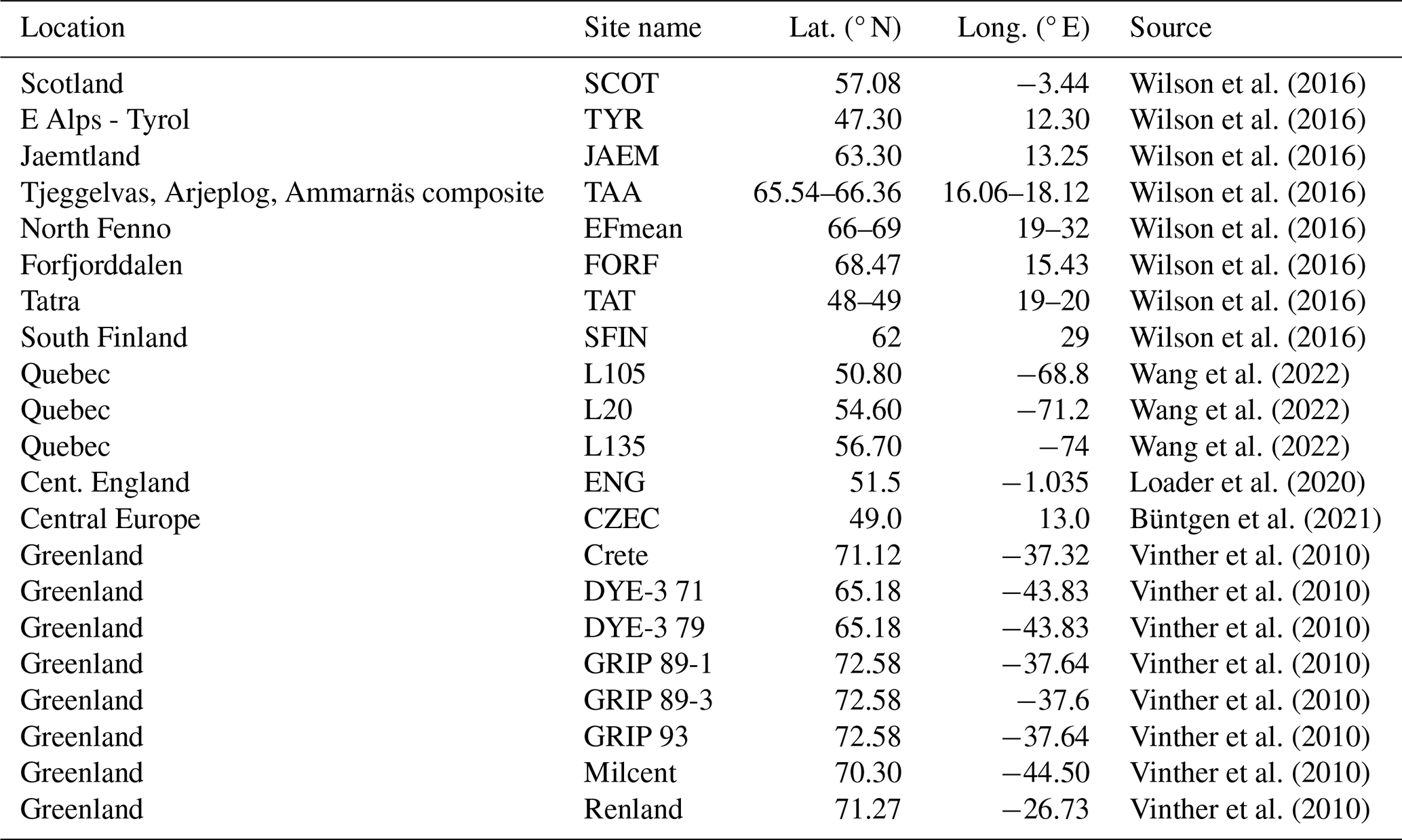
We select the proxy data with the following criteria. Firstly, the proxy data should have a strong imprint of climate. In case of the MXD, tree-ring width (TRW) and BI data from tree-ring chronologies, this means high correlation to local temperature, while we look for a clear imprint of atmospheric circulation in the δ¹⁸O-based records. Secondly, the proxy data needs to have 0–1-year dating uncertainty and a well-defined seasonality. To achieve consistent performance of the reconstruction, we only select proxy records that span the whole time frame of the reconstruction (CE 1241–1970) (Fig. 1 and Table 1).

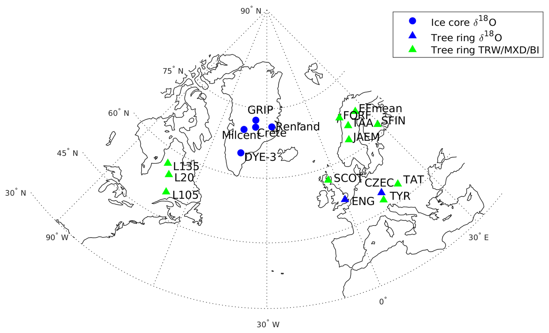
Figure 1 Sites for proxy data assimilated in the reconstruction. Geographical coordinates of sites and sources of data are listed in Table 1.

Wilson et al. (2016)Wilson et al. (2016)Wilson et al. (2016)Wilson et al. (2016)Wilson et al. (2016)Wilson et al. (2016)Wilson et al. (2016)Wilson et al. (2016)Wang et al. (2022)Wang et al. (2022)Wang et al. (2022)Loader et al. (2020)Büntgen et al. (2021)Vinther et al. (2010)Vinther et al. (2010)Vinther et al. (2010)Vinther et al. (2010)Vinther et al. (2010)Vinther et al. (2010)Vinther et al. (2010)Vinther et al. (2010)

Table 1 Proxy data sites assimilated in the reconstrution with coordinates and data sources listed.

The dating uncertainty of anchored tree-ring chronologies covering the past millennium is generally assumed to be zero. Furthermore, the sample replication of both the conventional and δ¹⁸O_cell tree-ring records featured in this study is stable throughout the reconstructed interval. The ice core data are dated using layer counting and synchronised using volcanic historically identified reference horizons, and for the past millennium the dating uncertainty is estimated to be maximum 1 year for the GICC05 chronology originally used for the high resolution ice core data (Vinther et al., 2006b). The volcanic dating horizons make it unlikely that the age scale of an entire ice core record shifted in time. However, one cannot exclude that some records are off by up to one year in some intervals between dating horizons, although the validity of the GICC05 time scale for the interval covering our reconstruction was confirmed by comparison to the updated GICC21 chronology (Sinnl et al., 2022).

We use the isotope enabled version of the climate model ECHAM5/MPIOM (Werner et al., 2016) run for the past 1200 years forced by natural and anthropogenic forcings. This is the same model simulation used in SEA18 and SEA20.

The atmosphere component is run in a T31L19 configuration corresponding to 3.75° × 3.75° horizontal resolution and 19 vertical layers, while the ocean component, MPIOM GR30L40, is set to 3° horizontal resolution with 40 layers. The model features isotope fractionation during all phase changes, including kinetic fractionation during evaporation and in mixed-phase clouds.

2.2 Interpretation of δ¹⁸O_cell

The variability of δ¹⁸O_cell is governed by several different processes, some of which have a high degree of co-variability. From the following analysis, we assume that the main control of δ¹⁸O_cell is the isotopic composition of precipitation forming the groundwater, which comprises the source water for formation of xylem sap used to form cellulose during the growing season. Depending on the hydrological setting at the site of the tree-ring chronology, there can be a lagged isotope signal from precipitation formed prior to the growing season, or from climate driven intra-annual variability. The lag can be due to groundwater recharge during spring snow melt or sap formed during late winter and spring (Wang et al., 2005). Our tests indicate that both δ¹⁸O_cell records used in this study are sensitive to weather variability (SLP, T2m, precip. amount) during the growing season (Fig. S1 in the Supplement), as well as the weather variability of the winter preceding the growing season (Fig. S2). The records ENG and CZEC are mainly correlated to variability connected to the winter NAO, which can be explained by the JJA Palmer drought severity index (pdsi) at these sites being sensitive to the DJF NAO. This is due to moisture availability of the growing season being affected by the preceding winter precipitation, as well as land-atmosphere feedback mechanisms where weather patterns promoting summer drought are enhanced by low soil moisture of the previous winter season (Wang et al., 2011). Based on these findings we use the δ¹⁸O_cell records as representing a mixture of summer and winter variability. The impact of large-scale circulation on weather variability and δ¹⁸O in precipitation weakens in spring, while the maximum correlation between δ¹⁸O_cell (ENG and CZEC, Table 1) and climate variables are seen in the growing season (Loader et al., 2020; Büntgen et al., 2021). We use JJA for representing the growing season and the extended winter season (November–April) to represent the winter preceding the growing season. Using the extended winter accounts both for impact of the winter circulation patterns, precipitation and composition groundwater for early spring sap formation. In addition, this choice of seasonal dependency the δ¹⁸O_cell is linked to the Greenland ice core data through the extended winter δ¹⁸O, and to the conventional tree-ring data through the co-variability of JJA temperature and δ¹⁸O. While a mechanistic approach to connect the δ¹⁸O_cell to δ¹⁸O in precipitation is possible through forward modelling (e.g. Roden et al., 2000), this would also introduce new parameters with uncertainties specific to each site. Since the untreated δ¹⁸O_cell in the first place has a clear imprint of atmospheric circulation for summer and winter, we choose to assume that the variability of δ¹⁸O_cell primarily is governed by a mix of δ¹⁸O in precipitation for both seasons.

2.3 Observations, reanalysis and reconstructions for validation and comparison

We use a variety of data ranging from instrumental data to climate field reconstructions to evaluate our climate reconstruction. For assessing spatial coverage of skill, we use the 20th Century Reanalysis version 3 (20CRv3) (Slivinski et al., 2021), which is only constrained by observations of SLP and sea surface temperature (SST). We furthermore compare to the HadCRUT5 gridded temperature (Morice et al., 2021) and the GPCC gridded precipitation (Schneider et al., 2022). As a supplement to evaluating the reconstruction with the 20CRv3 and HadCRUT5 temperature we use long-term observed temperature from Greenland (Vinther et al., 2006a), Iceland (Icelandic Met Office, 2026), England (Legg et al., 2025), Denmark (Cappelen et al., 2021) and Sweden (Moberg et al., 2002; Bergström and Moberg, 2002), to achieve a longer overlapping time interval for the evaluation. To evaluate reconstructed SST we use three different datasets ERSSTv5 (Huang et al., 2017), COBE2 (Hirahara et al., 2014), HadISST (Rayner et al., 2003) that have different properties due to different treatment of observational data and missing values. In addition to purely observation-based datasets, we compare our to the climate field reconstructions the Last Millennium Reanalysis (LMR) in annual (LMR v2.1) (Tardif et al., 2019) and seasonal resolution (LMR Seasonal) (Meng et al., 2025), as well as the ModE-RA reanalysis (Valler et al., 2024) of monthly resolution covering 1421–2008. In addition to proxy data, ModE-RA is assimilated based on instrumental data and historical documents.

2.4 Methods

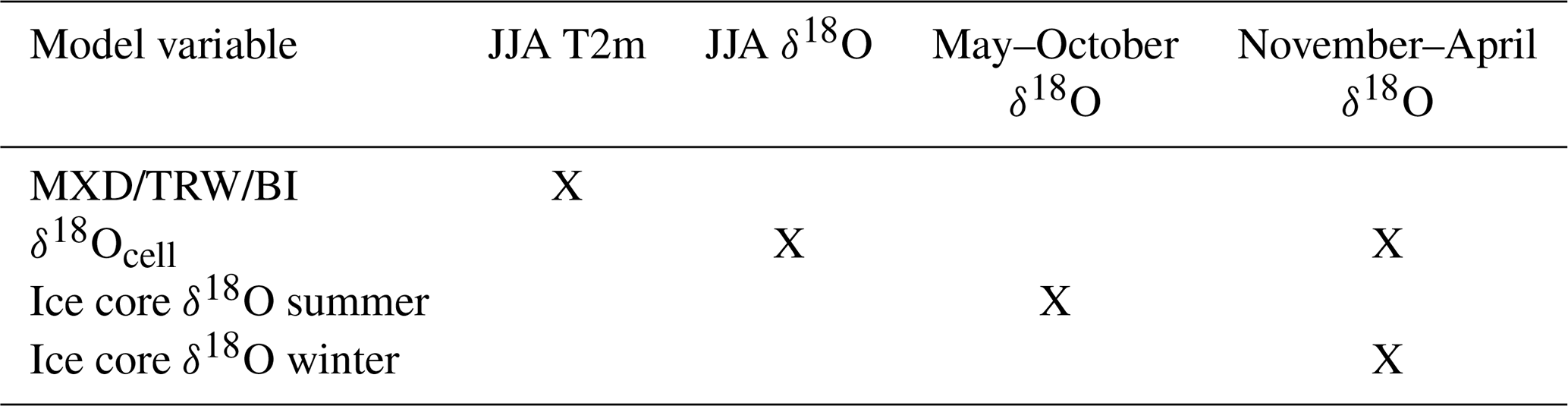
We use the analogue method to assimilate proxy data using an isotope enabled climate model. This setup can be described as assimilation with a static ensemble or static model prior. Building on experience of using this method effectively for previous reconstructions (SEA18/20), we expand the assimilated proxy network with new records and update the methodology for calculating the ensemble mean and introduce a variance correction. Our reconstruction is not calibrated against observations, and only relies on matching the model output with proxy data. For each site we evaluate the model output against the proxy data, linking simulated JJA temperature to conventional tree-data (MXD/BI/TRW), and simulated seasonal δ¹⁸O with ice core δ¹⁸O and δ¹⁸O_cell (Table 2). We use different evaluation criteria of the model data for the summer and winter season. For the summer season we use a χ²-measure for the goodness of fit:

$$\begin{array}{}\text{(1)}& {\mathit{\chi }}_{\mathrm{sum}}^{\mathrm{2}}\left(t\right)=\sum _{i=\mathrm{1}}^n{\displaystyle \frac{{\left(m(n,t^{\prime })-p(n,t)\right)}^{\mathrm{2}}}{{\mathit{\sigma }}_{\mathrm{mp}}}},\end{array}$$

where, m is the modelled anomaly and p is the proxy anomaly at a given site, n is the number of proxies, t is the year of the reconstruction, t^′ is the year of the model run, and σ_mp is the combined standard deviation of the model and proxy data. Dividing by σ_mp normalizes the data, which is effectively the same as normalizing all time series (proxy data and model output for proxy sites) prior to the matching procedure.

Table 2 Proxy parameters and corresponding model variables used in matching model output to proxy data.

The imprint of large-scale circulation on the isotopic composition is very strong for winter and the amplitude of the δ¹⁸O anomalies bears a signal in it-self. Part of this signal is the gradient between proxy sites (Sjolte et al., 2018). Since we are interested in preserving as much of the signal in the proxy data as possible, we do not normalize the data when fitting the model data to the proxy data. The measure for goodness of fit for winter is then:

$$\begin{array}{}\text{(2)}& {\mathit{\chi }}_{\mathrm{win}}^{\mathrm{2}}\left(t\right)=\sum _{i=\mathrm{1}}^n{\left(m(n,t^{\prime })-p(n,t)\right)}^{\mathrm{2}},\end{array}$$

where, m is the modelled anomaly and p is the proxy anomaly at a given site, n is the number of proxies, t is the year of the reconstruction and t^′ is the year of the model run.

The workflow for the annual and seasonal reconstructions is illustrated in Fig. 2. For the seasonal reconstructions we reconstruct the summer and winter separately using Eqs. (1) and (2), respectively, while for the annual mean and monthly reconstruction, the proxies for summer and winter are matched simultaneously using Eq. (1). The monthly data from the best matching model years are then extracted, taking into account that the ice core data for winter are representing months November–April when the annual mean for the calendar mean is calculated (i.e., November–December are assigned to previous calendar year compared to the matched winter proxy data centred in January). As we have no direct constraints on monthly data, we mainly include the monthly reconstruction to be able to investigate the seasonality of SAT25 and compare with other datasets.

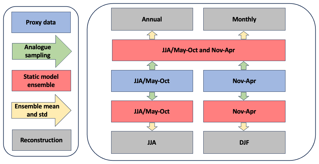
Figure 2 Flow diagram showing the differences in data treatment between the seasonal and annual (monthly) reconstructions. The legend on the right shows the colour coding of datasets (squares) and processing (arrows).

In this study we calculated the ensemble mean using a logarithmic weighting function. Due to the bias-variance trade off, a high number of ensemble member reduces noise and increases skill in term of correlation but causes decrease in variability, as well as skewing the variability towards the main mode and causing mixed secondary modes in the SLP field. Before arriving at our current approach, we tested different ways to calculate the ensemble mean: constant number of ensemble members with equal weighting (as SEA18/20), variable number of ensemble members based on match with proxy data, also in combination with a minimum number of ensemble members. Here we calculate the weighted mean based on the χ² fit (Eqs. 1 and 2), which yields a smoother behaviour of reconstruction with less year-to-year difference in the statistical properties of the reconstruction compared to a variable number of ensemble members, while still allowing the best matching models years to have the most weight. The weighting is calculated as the logarithm of the normalized χ²-distance, where the least important ensemble member receives zero weighting (Fig. S3). The χ²-distance as a function of number of ensemble members is similar to an exponential decay function and we apply the logarithm to achieve a more equal weighting of the ensemble members. Otherwise, the result would be skewed too much towards a few of the best fitting ensemble members, which results in more noise in the reconstruction. With the applied weighting 50 % of the weight goes to the best matching 30 % of the ensemble members.

In our results we show time series as anomalies from the mean of the full-length data series, and monthly data are anomalies with respect to the mean annual cycle. We use Pearson correlation (r) and significance levels are determined using Student's t test. For correlation maps we list the maximum correlation, mean significant correlation and number of grid cells with significant correlation below the figure title. The number of grid cells with significant is a rough indication of the spatial coverage of the skill, which will depend on the spatial auto-correlation, which in turn depends on season, latitude (area of grid cell) and type of climate variable. For the point-wise correlation maps all data from reanalysis, observations and climate field reconstructions are re-gridded to the 3.75° × 3.75° grid used for SAT25.

3 Results

3.1 Ensemble reconstruction and initial evaluation

Before comparing to observed climate we evaluate the coherence between the reconstruction and the assimilated proxy data, and assess how many model analogues per year to use in the ensemble reconstruction. When determining number of ensemble members to include for each year there are several factors to consider. A high number of ensemble members reduces noise by smoothing the variability spatially and temporally, but as mentioned above, the smoothing also makes it more difficult to separate the main modes of climate variability. For example, with a high number of ensemble members, the East Atlantic and Scandinavian blocking patterns cannot be separated and more of the variability is assigned to the NAO. Conversely, a low number of ensemble members fail to span both the imperfect fit of the model to the proxy data, as well as the confounding noise of the proxy data.

We first consider the match between the reconstructed signal at the sites of the proxy data. There is high correlation between the reconstruction and all proxy records, with a match to ice core δ¹⁸O and δ¹⁸O_cell in the range r ∼ 0.65–0.9, and on average slightly better correlation between reconstructed temperature and conventional tree-ring records, though in similar range (r ∼ 0.6–0.9). We tested the match with proxy data with increasing number of ensemble members. The maximum correlation to proxy data is achieved with 10–100 ensemble members per year, however the match to the proxy data only degrades slowly with up to 300 ensemble members per year due to the weighting with respect to χ²-distance to the proxy data (Fig. S4). Using 300 ensemble members introduces spatial smoothing which filters out noise in particularly for areas far from the proxy sites (see Sect. 3.4). With this high number of ensemble members, we on one hand lose information on modes of atmospheric circulation, as mentioned in the introduction, but on the other hand gain skill for basin-wide variability for the North Atlantic region. We therefore provide two versions of the reconstruction, one using 150 ensemble members and one using 300 ensemble members. For simplicity we focus on the version with 300 ensemble members as the differences are subtle and will be explored in future work.

Previous seasonal reconstructions (SEA18/20) only used ice core data, or introduced tree-ring data after a pre-selection of model analogues had been made using ice core data. Here we fully incorporate the tree-ring data. The match with ice core records can be achieved regardless if the tree-ring data is included or not, indicating that the analogue sampling pool is sufficiently large to provide relevant analogues, and that further constraining the climate variability with records in Europe does not hinder a good match over Greenland.

To further test the role of the tree-ring and ice core data, we made two new reconstructions based on our annual reconstruction. One based only on ice core data (RECON_IC) and once based only on tree-ring data (RECON_TR). We then extracted the data for tree-ring sites from RECON_IC and the ice core sites from RECON_TR. The results show that the prediction of tree-ring variability from RECON_IC has weak skill, although some correlations are significant (see Figs. S5–S8). The best correspondence is seen for Scandinavian tree-ring records (TAA, EFmean) and winter δ¹⁸O correlated to CZEC δ¹⁸O_cell. Conversely, the prediction of ice core variability from RECON_TR also has weak skill (Figs. S9 and S10), with the best correlation to GRIP δ¹⁸O (r = 0.33) (Fig. S9). This underlines the different properties of the proxy data due to differences in seasonality, region and what is recorded by the proxies. In broad terms, the main strength of the ice core data is to record large-scale atmospheric circulation for winter, while the tree-ring data capture temperature changes on a more local scale, but the wider availability of tree-ring data ensures a reasonable spatial coverage to capture a large-scale summer signal. Our main conclusion from this test is that the properties of the different sets of proxy data are complementary and constrain different seasons and regions of the reconstruction.

The uneven distribution of proxy data concentrates skill and variance near the sites of the proxy data, and calculating the ensemble mean dampens the overall variance. We bias correct the variance of the reconstruction by rescaling the standard deviation of each grid point with the corresponding standard deviation of the ECHAM5-wiso/MPIOM run. Our motivation is that the climate model acting as the model prior is the best estimate of the variance in locations not constrained by proxy data. This very simple correction improves the match between reconstructed variance compared to the variance for SLP, T2m and precipitation from 20CRv3 (Figs. S11 and S12).

To test the long-term stability of the reconstruction we investigated temporal variations of the match with proxy data. The average fit of model analogues is fairly constant over time, indicating that the quality of the climate reconstruction is consistent throughout 1241–1970. One reason for this consistency is the strict selection of proxy records that span the whole reconstruction, which means that there are no methodological differences throughout the reconstruction. We found no clear preference with respect to selection of model analogues throughout the reconstruction. This is consistent with results for earlier versions of the reconstruction (SEA18/20).

3.2 Comparison to meteorological reanalysis

SEA25 is not calibrated to observations (see Sect. 2.4). The comparison to observed climate in this section is therefore an independent measure of skill. In addition, since we use a constant number of proxy data and no change in methodology throughout the reconstruction, we should, in theory, reach the same level of skill for any time period of the reconstruction.

Compared to the JJA and DJF mean for 20CRv3, the reconstruction shows coherent patterns of skill for SLP and T2m, while the skill for precipitation is patchier (Fig. 3). Standout features are widespread significant correlation for the winter SLP and strong correlation over the eastern North Atlantic and Northern Europe for summer T2m (max. r = 0.71). In winter the level of correlation is tightly connected with the skill for reconstructed circulation patterns. This is especially clear for the winter SLP and T2m which resemble the spatial pattern of NAO-type variability, while summer SLP and T2m which resemble the spatial pattern of Scandinavian blocking-type variability. The weaker skill for summer circulation is due to a combination of less well constrained large-scale circulation during summer and biases in the JJA SLP patterns of the ECHAM5/MPIOM model (Sjolte et al., 2020). An alternative to Fig. 3 replacing the 20CRv3 data with HadCRUT5 for temperature and GPCC for precipitation can be found in the Supplement (Fig. S13). These results are comparable to the comparison with 20CRv3, although the correlation to HadCRUT5 is somewhat better.

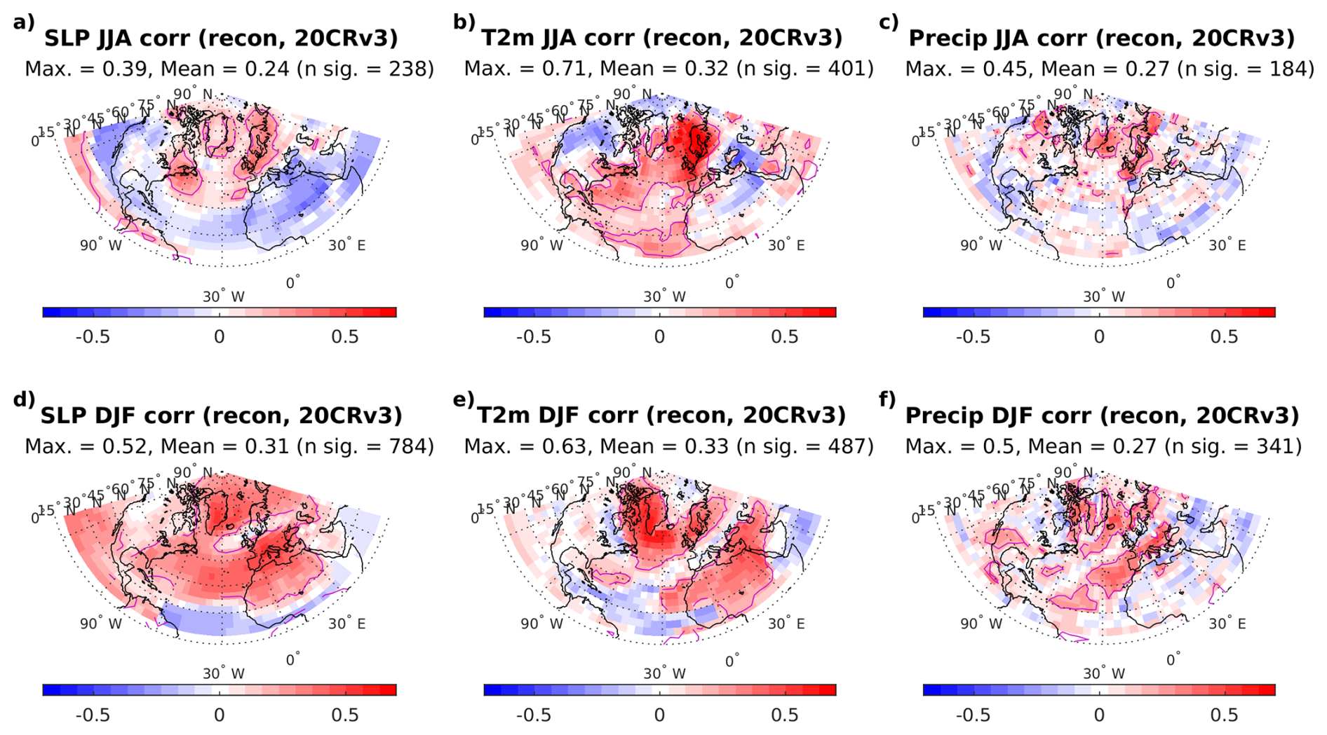
Figure 3 Point-wise correlation for CE 1850–1970 between reconstructed and 20CRv3 SLP, T2m and precipitation for JJA mean (a–c) and DJF mean (d–f) data. The maximum correlation, mean significant correlation and number of grid points with significant correlation are indicated for each subplot. Contour indicates p = 0.01.

The correlation patterns for the annual mean are, not surprisingly, a combination of features seen for summer and winter (Fig. 4a–c). While it is less pronounced than for DJF, the signature of NAO-type variability is still evident in the spatial patterns of the correlation. The maximum correlation (r = 0.68) is achieved for T2m with lower correlations for SLP and precipitation than for winter, indicating that auto-correlation in temperature aids higher skill in some areas, while the seasonal information is lost in the annual mean SLP and precipitation due to shifting circulation patterns and different impact of circulation on T2m and precipitation on a seasonal scale.

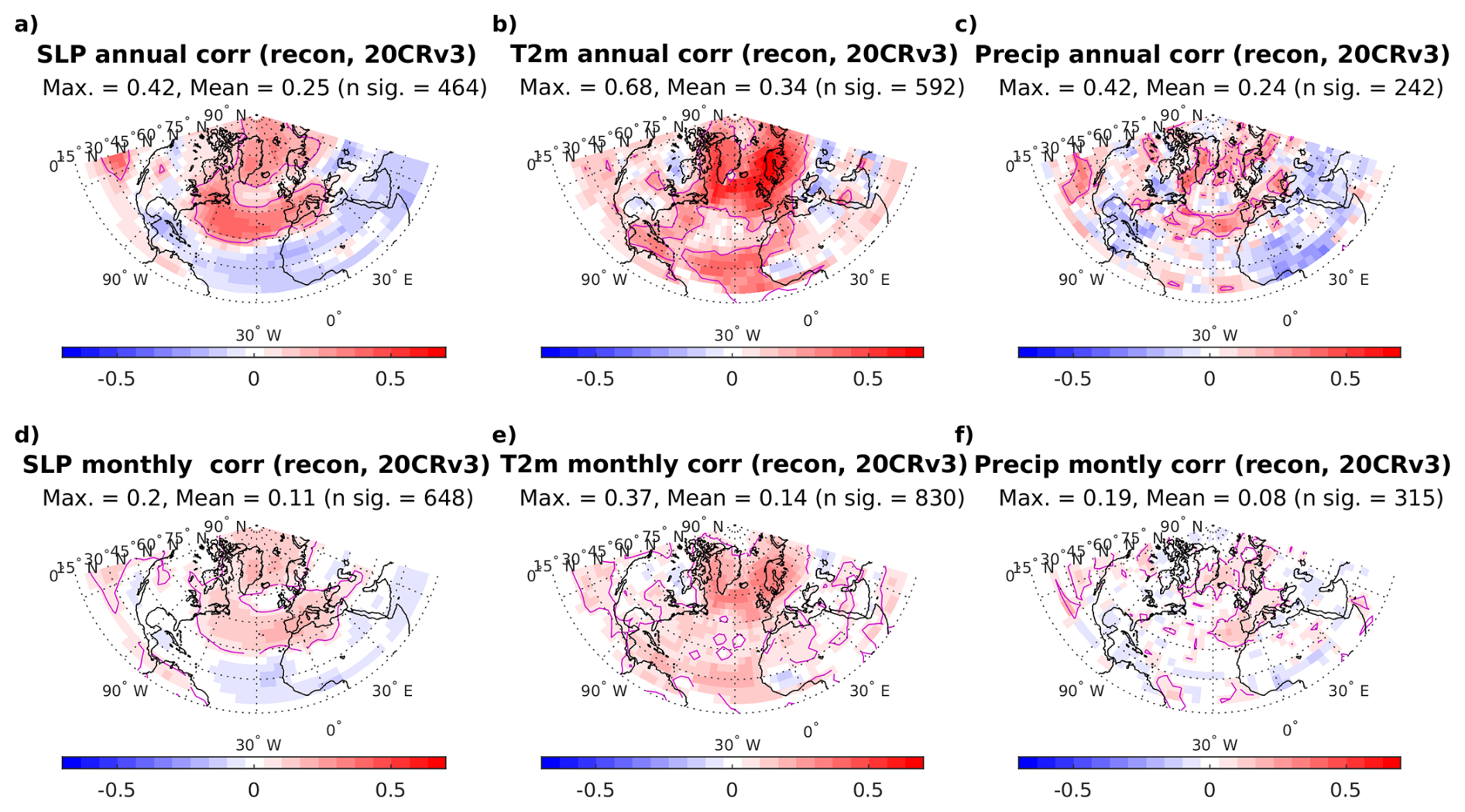
Figure 4 Point-wise correlation for CE 1850–1970 between reconstructed and 20CRv3 SLP, T2m and precipitation for annual mean (a–c) and monthly mean (d–f) data. The maximum correlation, mean significant correlation and number of grid points with significant correlation are indicated for each subplot. Contour indicates p = 0.01.

On monthly time scales the skill of the reconstruction is lower with at maximum correlation of 0.34 for T2m (average for all months) (Fig. 4d–f). Despite lower skill, the correlation is still significant over large areas, due to the larger sampling pool (12 times as more sample points compared to annual data). The spatial patterns of the correlation are similar to that of the annual mean reconstruction. Reviewing the skill for individual months, correlations peak in February and August for T2m with maximum correlation with 20CRv3 of 0.55 and 0.70, respectively (Fig. S14). Again, the comparison the HadCRUT5 monthly temperature shows somewhat higher correlation than to 20CRv3 (Fig. S15). For SLP the imprint of large-scale circulation is again evident during winter months (max. corr. = 0.38 for February) with lower and more localized skill during summer (not shown). A summary of the SAT25 correlation to monthly 20CRv3 data can be found in Fig. S16. The skill for the monthly reconstruction varies regionally due to the seasonality of the proxy data and seasonal shifts in climate patterns, leading to summer months and winter months not having high skill at the same location. For example, this is part of the reason for the annual average monthly temperature correlations to remain low, although they peak above 0.6 for temperature during July and August (Fig. S16).

3.3 Comparison to long-term temperature records

In addition to the comparison with 20CRv3 we compare to observed temperature from Greenland, Iceland, Central England, Denmark, and Sweden which are among the longest observed high-quality temperature records and span our study area well. For summer the high skill of the reconstruction seen in Fig. 3b is confirmed for sites in Sweden and England (Fig. 5). It appears that there are periods of over and underestimated reconstructed temperature which could be a sign of underestimated multi-decadal variability, or it could be due to a different long-term trend in the reconstruction. However, for Uppsala, which is close by Stockholm and has a longer observational record, the reconstruction shows the highest correlation to observed summer temperature (r = 0.56). It is also reaffirming that the reconstruction shows good correlation to the longest existing instrumental record, the Central England temperature (r = 0.5). The lower skill for Greenland sites during summer is similar to earlier studies, because Greenland ice core summer δ¹⁸O is more sensitive to climate variability east of Greenland, also illustrated by good correlation to Iceland summer temperature (r = 0.54) (Vinther et al., 2010; Sjolte et al., 2020). Due to a bias of the model prior, the variance in Southern Greenland is underestimated for summer, which can be seen in the reconstructed time series from Qaqortoq (Fig. 5) and in the map of the standard deviation of reconstructed temperature (Fig. S11).

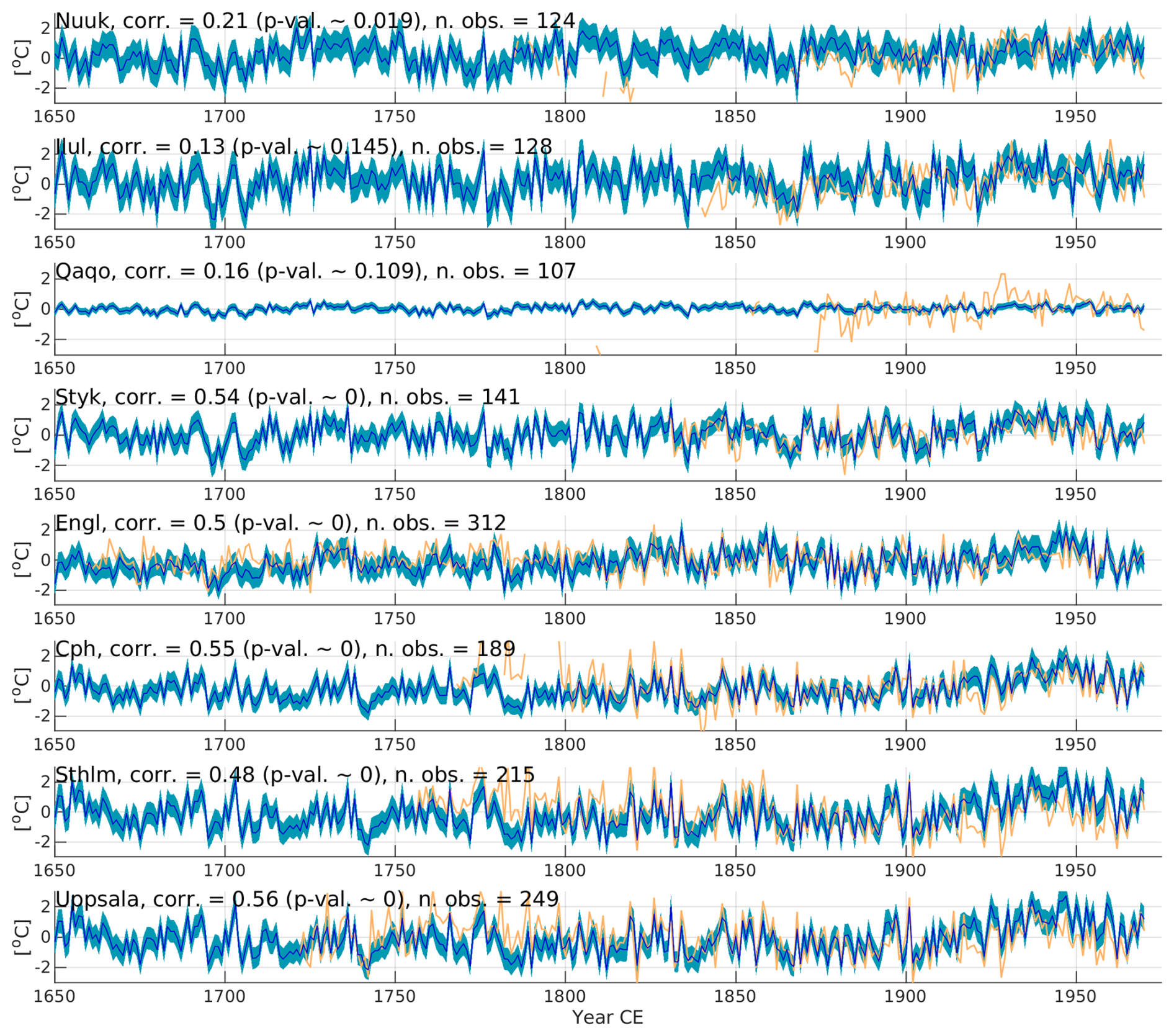
Figure 5 JJA temperature: time series of reconstructed (blue) and observed (yellow) temperature for Nuuk, Ilulissat, Qaqortoq, Stykkishólmur, Central England, Copenhagen, Stockholm, and Uppsala. The correlation (corr.) and number of months in the observations (n. obs.) are indicated for each site. The blue shading indicated ±1 SD of the ensemble reconstructed temperature.

The highest skill during winter is seen for Greenland winter temperatures (r ∼ 0.6), although we also see good performance for Stockholm (r = 0.46), despite having no proxy site nearby (Fig. 6). Compared to summer there are only the two δ¹⁸O_cell proxy sites available for the winter season besides the Greenland ice cores. However, this is partly counteracted by the stronger impact of large-scale circulation on regional climate variability enabling good skill also in the Eastern part of the study area. We observe that the variance for DJF is approximately double of the JJA variance. This is captured well for most sites by the reconstruction, also showing that the variance correction is effective also compared to instrumental data.

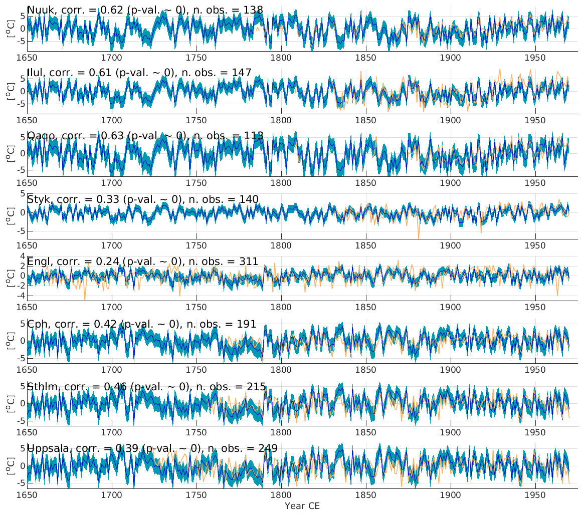
Figure 6 DJF temperature: time series of reconstructed (blue) and observed (yellow) temperature for Nuuk, Ilulissat, Qaqortoq, Stykkishólmur, Central England, Copenhagen, Stockholm, and Uppsala. The correlation (corr.) and number of months in the observations (n. obs.) are indicated for each site. The blue shading indicated ±1 SD of the ensemble reconstructed temperature.

For annual mean data the correlation is more consistently in the range of 0.5–0.6 (Table 3), again, combining the characteristics of the summer and winter season, as well as capturing amplitude of the temperature variance (Fig. S17).

Table 3 Correlation to Long-term temperature observations for the annual, JJA, DJF, and monthly mean. Boldface marks significant correlations with p < 0.01.

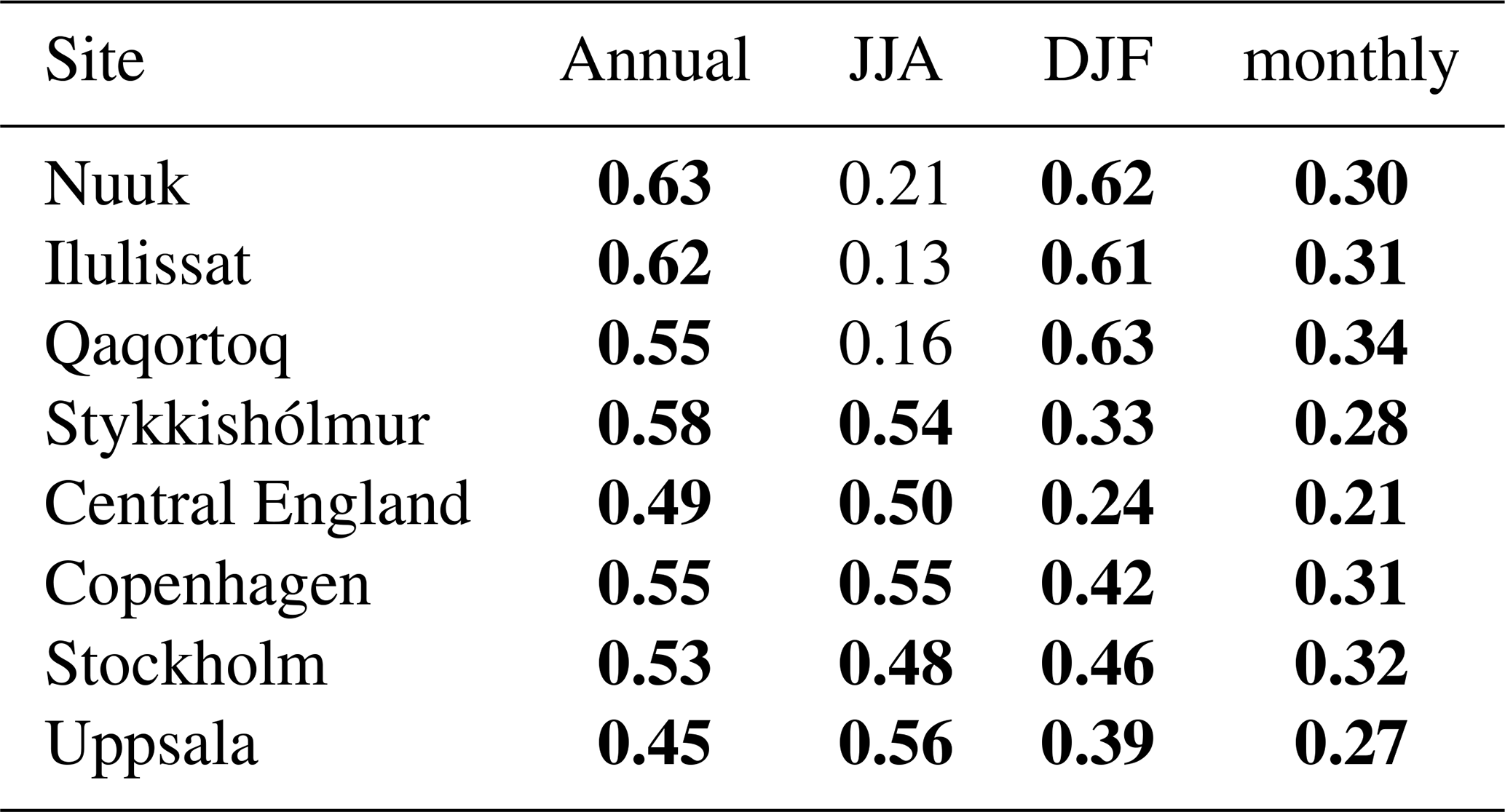
The monthly reconstruction has correlations of ∼ 0.3 at all sites but for Central England which has lower correlation (r = 0.21). The lower skill for Central England is likely due to the winter variability being less coupled to the NAO. As the reconstruction is not constrained at monthly resolution, we cannot expect high skill on a month-to-month basis. What we do see is the reconstruction capturing part of the modulation of the annual cycle seen in the observations. For example, for the cold winters during the 16th and 17th century in Scandinavia (Fig. S18).

3.4 Annual mean SST evaluation

The annual reconstruction, which targets the calendar year, enables direct comparison to more common annual reconstructions and is useful for analysing indices of sea surface temperature which are often defined on annual mean data. Our reconstruction uses a high number of ensemble members (300, ∼ 25 % of the available model analogues) introducing spatial smoothing to filter out noise in particular for areas far from the proxy sites. Using this high number of ensemble members, we on one hand lose information on modes of atmospheric circulation, as mentioned in the introduction, but on the other hand gain skill for basin-wide variability for the North Atlantic region (Fig. 7).

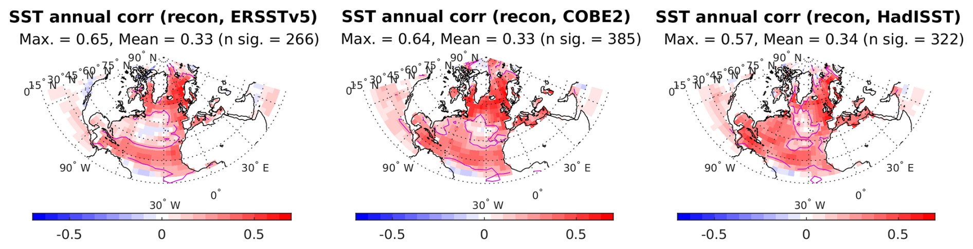
Figure 7 Reconstruction of annual sea surface temperature (SST) correlated point-wise to three different SST datasets based on observations (ERSSTv5 1870–1970, COBE2 1850–1970, HadISST 1854–1970). Contour indicates p = 0.01.

3.5 Comparison to climate field reconstructions

In this section we compare to climate field reconstructions of annual, seasonal and monthly resolution. The Last Millenium Reanalysis (LMR) SLP, temperature and precipitation amount is available in annual resolution (Tardif et al., 2019), as well as seasonal resolution for temperature (Meng et al., 2025). Both the annual and seasonal resolution LMR span the entire time period of our reconstruction. The ModE-RA reanalysis is one of the few monthly resolution paleo-reanalysis datasets and covers 1421–2008 (Valler et al., 2024).

The annual mean SLP, temperature and precipitation of our reconstruction correlates well with the annual mean LMR data if we compare the full time period of the reconstruction (CE 1241–1970) (Fig. 8a, b, c), showing similar or better correlation than to the 20CRv3. For seasonal temperature there is a strong coherence between SAT25 and LMR for JJA temperature with maximum correlation of 0.9 over Northern Europe (Fig. 8d), while there is no correlation over Greenland. The correlation during winter reaches 0.59 (Fig. 8e), which is just below the DJF correlation of SAT25 to 20CRv3.

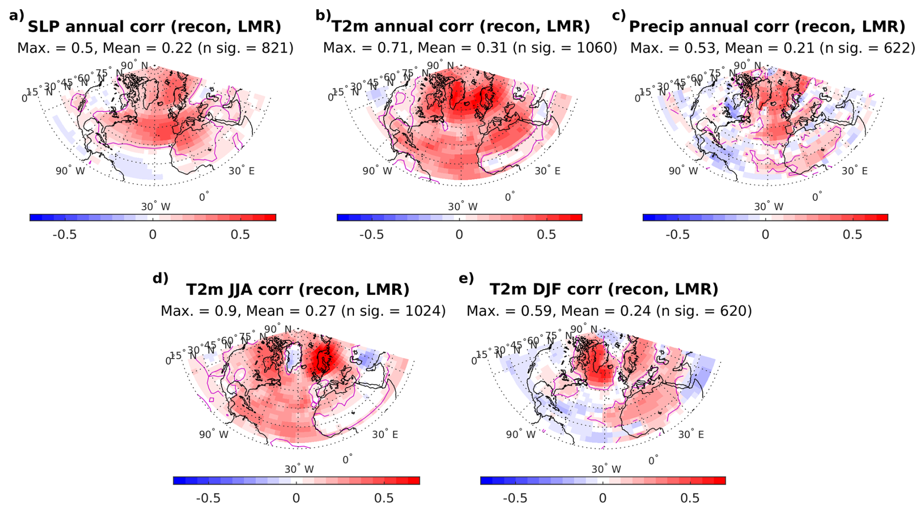
Figure 8 Point-wise correlation for CE 1241–1970 between SAT25 and the Last Millennium reanalysis (LMR) SLP, T2m and precipitation for annual mean (LMR v2.1) (a–c) and seasonal T2m mean (LMR Seasonal) (d–e) data. The maximum correlation, mean significant correlation and number of grid points with significant correlation are indicated for each subplot. Contour indicates p = 0.01.

For the comparison to seasonal means of the ModE-RA reanalysis of the full overlapping time period (1421–1970) we see similar correlations as to the 20CRv3 for JJA SLP and temperature, while the coherence to JJA precipitation is weaker (Fig. 9a, b, c). The correlations to the ModE-RA DJF mean are lower than for the comparison to the correlations to DJF 20CRv3 (Fig. 9d, e, f). Comparing our reconstruction and ModE-RA temperature in monthly resolution for the full overlapping time period 1421–1970, we see comparable results as for correlation to 20CRv3 for the summer months, showing large areas of coherent correlation over the North Atlantic (Fig. 10). In contrast, the winter months show lower correlation than to 20CRv3 between the two reconstructions.

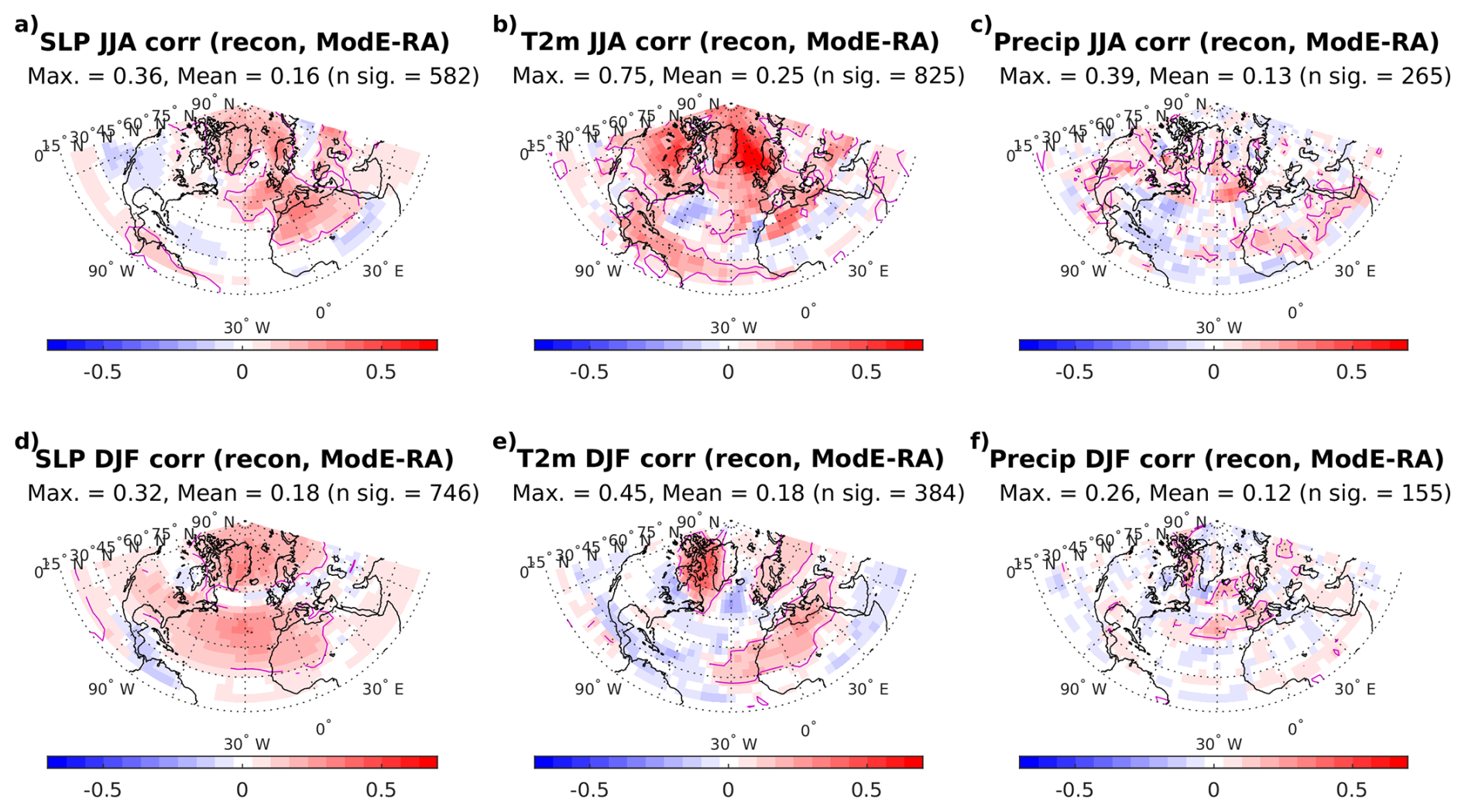
Figure 9 Point-wise correlation for CE 1421–1970 between SAT25 and ModE-RA SLP, T2m and precipitation for JJA mean (a–c) and DJF mean (d–f) data. The maximum correlation, mean significant correlation and number of grid points with significant correlation are indicated for each subplot. Contour indicates p = 0.01.

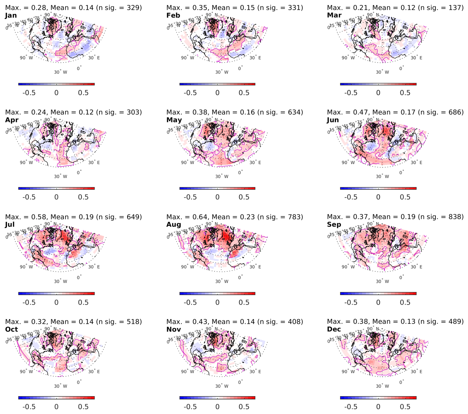
Figure 10 Point-wise correlation for CE 1421–1970 between SAT25 and ModE-RA monthly T2m. The maximum correlation, mean significant correlation and number of grid points with significant correlation are indicated for each subplot. Contour indicates p = 0.01.

Next, we investigate the long-term variations of co-variability between SAT25 and the LMR and ModE-RA climate field reconstructions by looking at the correlation in 121-year time windows, providing similar properties as the comparison with the overlapping time period with the 20CRv3 (1850–1970). The results are summarized in Fig. 11 by plotting the maximum correlation and number grid points with significant correlation for annual and seasonal means for six time windows covering 1250–1970 for the LMR data, and four time windows covering 1490–1970 for the ModE-RA reanalysis (see Figs. S19 to S24 for all correlation maps). The maximum correlation shows larger excursions than the mean significant correlation, and is used in Fig. 11 as an effective indicator of strength of the co-variability between the different datasets. For reference, we also plot the JJA and DJF maximum correlation and number grid points with significant correlation from the 20CRv3 comparison. The correlations to LMR remain rather stable over time, although generally highest in the most recent time window (1850–1970) and lowest in the earliest part of the reconstruction (1250–1370) (Fig. 11a). While more variable, this pattern is also reflected in the number of grid points with significant correlation, although the relation between SAT25 and LMR annual SLP is relatively stable (Fig. 11b). Apart from the moderate long-term trend of decreasing coherence between SAT25 and LMR going back in time, the intervals covering 1490–1730 display somewhat variable correlation between the reconstructions. For example, the correlation to LMR DJF temperature is lowest for this time frame, coinciding with a shift in the correlation to LMR annual SLP, while the correlation to LMR JJA and annual temperature remains high.

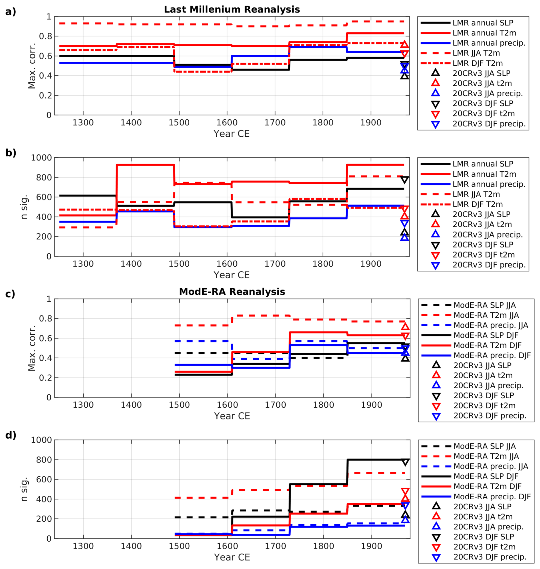
Figure 11 Maximum correlation and number of grid points with significant correlation in 121-year intervals between SAT25 and the Last Millennium Reanalysis in annual (LMR v2.1) and seasonal (LMR Seasonal) resolution (a, b), and between SAT25 and the ModE-RA reanalysis (c, d). The results from the correlations between seasonal SAT25 and 20CRv3 from Fig. 3 is shown for reference. The correlation maps for all time intervals are show in Figs. S19–S24.

The results for the stability of the correlation to the ModE-RA reanalysis contrast the results of the comparison to the LMR, as they show a clear decrease in coherence going back in time (Fig. 11c and d). This is most prominently seen as an almost complete loss of coherence between SAT25 and the ModE-RA DJF variability, going from correlations similar to the 20CRv3 in the most recent interval (1850–1970), to very little correspondence in variability for the earliest interval (1490–1610).

4 Discussion and conclusions

Compared to the SEA18/20 reconstructions, our new reconstruction shows several clear improvements in the performance for summer and winter. This includes more wide-spread skill for all reconstructed variables and more realistic variance due to a simple, but effective, variance correction. With the introduction of the variance correction, the performance of the reconstruction is significantly improved in comparison with the 20CRv3 and observed temperature records. This indicates that the reconstruction will lend itself well to studies of forcing attribution, climate extremes and model evaluation given the more realistic amplitude of changes featured in the reconstruction. Furthermore, we included reconstructions in annual and monthly resolution. The calendar year is a widely used format in other reconstructions, and we include this to make comparisons to existing datasets more straight forward. Similarly, our monthly reconstruction can be useful when compared or used with other data if a specific seasonality is targeted, which then can be a combination of any months. Finally, we also included reconstructed precipitation as an output variable.

In Sect. 3.5 we compared SAT25 to other climate field reconstructions. The comparison to the LMR in annual and seasonal resolution shows fairly stable correlations through time, although we identified two time periods of lower correlation: the intervals 1490–1730 and the interval 1250–1370. From the results there are indications that there is a seasonal signal in the time periods of weaker correlation between SAT25 and LMR. Due to SLP is not being available from the seasonal resolution LMR, we investigate further by correlating the JJA and DJF of SAT25 to the annual LMR. The results are summarised in Fig. 12, where we also show the SAT25 T2m correlations to LMR Seasonal from Fig. 11 for reference (see Figs. S21, S22 and S25 to S28 for all correlation maps). The results for correlating the JJA/DJF SAT25 temperature to annual LMR have strong similarities to the results for comparing SAT25 to the seasonal resolution LMR, indicating that although the comparison of JJA/DJF data to annual data is not optimal, it does offer usable information. For example, we can observe that the shift 1490–1730 in the correlation patterns for annaul SLP most likely originates in a shift in the representation of the DJF large-scale SLP variability, also explaining the shift in the DJF temperature correlation patterns in the same intervals. Furthermore, we can see that the decrease in correlation for the 1250–1370 is most likely isolated to the summer season. The main conclusion from this is, that there is indeed no strong trend back in time in the correlation between SAT and LMR, though there are fluctuations in the correlation patterns between the reconstructions.

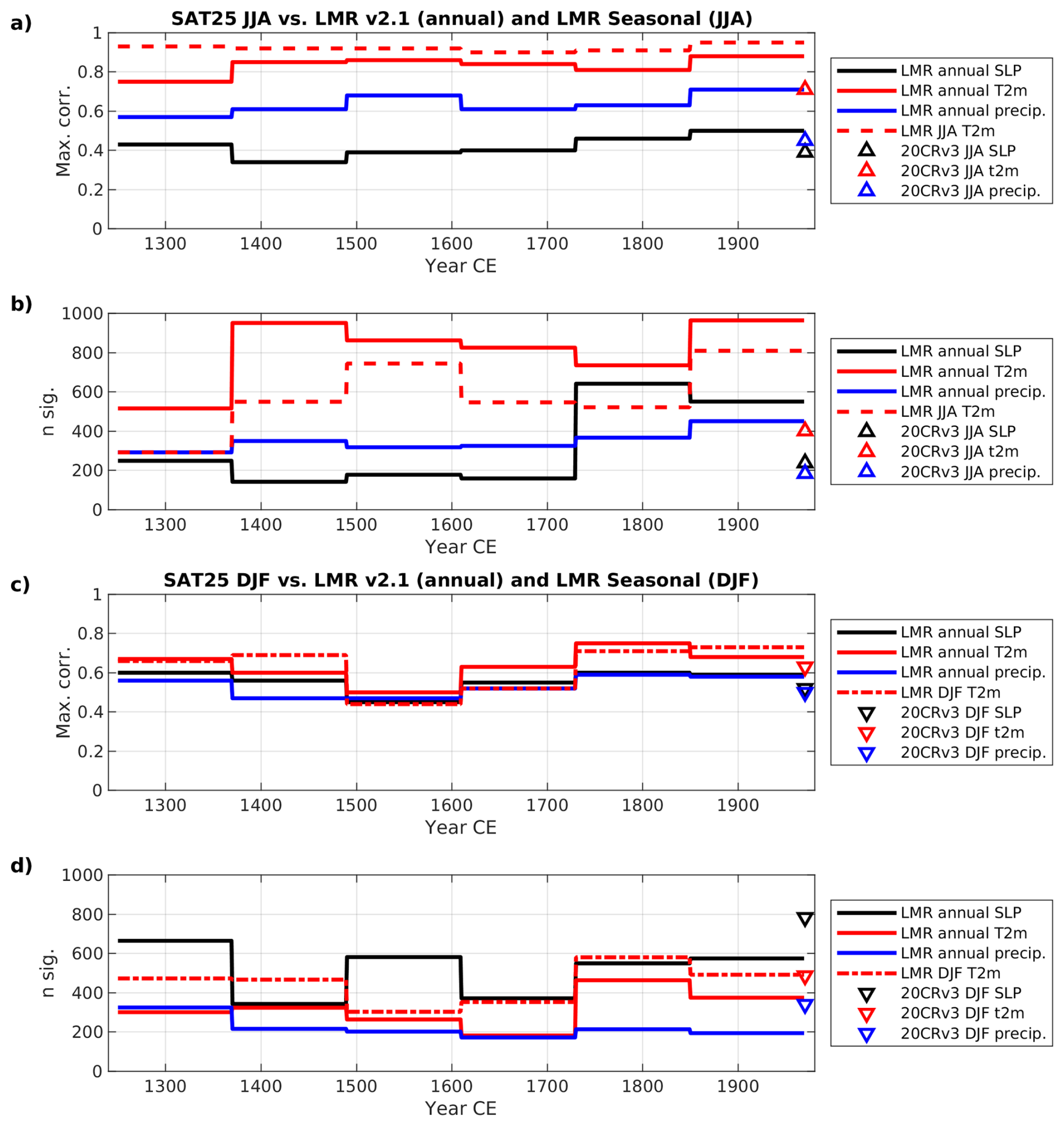
Figure 12 Maximum correlation and number of grid points with significant correlation in 121-year intervals between JJA SAT25 and the Last Millennium Reanalysis in annual (LMR v2.1) and seasonal (LMR Seasonal) resolution (a, b), and between DJF SAT25 and the Last Millennium Reanalysis in annual (LMR v2.1) and seasonal (LMR Seasonal) resolution (c, d). The results from the correlations between seasonal SAT25 and 20CRv3 from Figure 3 is shown for reference. The correlation maps for all time intervals are show in Figs. S21–S22 and S25–S28.

Non-stationary relationships between reconstructions can have a number of causes. In this study we have made an effort to produce a consistent reconstruction though time, by only including proxy records that span the whole time frame of the reconstruction. This contrasts the approach of the LMR and ModE-RA reconstructions where the amount of proxy data, and the case of ModE-RA, also documentary and instrumental data, decreases back in time. The main source for proxy data in the LMR reconstructions is the PAGES2k database (PAGES2k Consortium, 2017) and ModE-RA uses both the PAGES2k and Iso2k databases (Konecky et al., 2020). There is an overlap in the proxy data used for SAT25 and the LMR and ModE-RA reconstructions, in particularly for the tree-ring data. For ice core δ¹⁸O data, the PAGES2k database contains mainly annual data and a few ice cores sensitive to summer temperature. The Iso2k database has two ice core records representing winter (GRIP and Crete), which are the only ice core records targeting the winter variability in the ModE-RA reanalysis prior to CE 1778. For example, the Dye-3 data (annual resolution) used in ModE-RA does not go further back than CE 1778. In addition, the bulk of observational and documentary data used in ModE-RA mainly covers the time after CE 1800. We therefore find that one possible explanation for the loss of coherency in the earliest intervals of the comparison between SAT25 and ModE-RA is the decrease in number of records constraining the ModE-RA reanalysis prior to CE ∼ 1800. Additionally, the long-term variability of ModE-RA is governed by the model prior due to a 71-year assimilation window (Valler et al., 2024). This could also account for some of the discrepancy between the reconstructions. The LMR reconstructions uses several ice core δ¹⁸O records from the PAGES2k database, including Dye-3 δ¹⁸O. While these are primarily of annual resolution, they do cover the entire past millennium, explaining the relatively stable correlation between SAT25 and the LMR reconstructions.

Other factors in non-stationary relationships between reconstructions, are shifts in large-scale climate patterns or changes in importance (explained variance) of climate patterns, influencing the regional impact on climate variables and the variability recorded in proxy records. Having a larger network of proxy records, such as used in the LMR reconstructions, should make the reconstruction less sensitive to shifts in the influence of climate patterns. On the other hand, seasonal data provides better constraints on the seasonality of large-scale patterns and enables separation of seasonal climate variability.

A third factor in the comparison between climate field reconstructions is the model prior. In general, we see the best correspondence between reconstructions close to common proxy sites. For example, the high correlation in Northern Europe for JJA or annual data. Further away from proxy sites the inherent spatiotemporal patterns of the model prior partly determine the variability. Furthermore, SAT25 uses an isotope enabled model prior to provide a more direct link to the isotope-based proxy records, while the LMR and ModE-RA reconstructions uses regression-based calibration to observed climate.

Finally, the assimilation techniques play a role in the differences in climate reconstructions. For SAT25 we use the analogue method, building on previous experiences with this method (Sjolte et al., 2018, 2020). Opposed to Bayesian data assimilation techniques, such as Kalman filter-based algorithms used by the LMR and ModE-RA reconstructions, our approach does not include probabilistic treatment of proxy errors nor does it produce a statistically optimal ensemble mean. However, the analogue method has been found suitable for producing reconstructions for the common era (Gómez-Navarro et al., 2017).

In summary, the comparison of SAT25 to the LMR and ModE-RA reconstructions shows some of the differences in their properties, indicating that they are suitable for different applications. While SAT25 is limited to the North Atlantic region, it offers seasonal resolution in SLP, temperature and precipitation, which is not available from the LMR reconstructions, and SAT25 has a longer time span than the ModE-RA reanalysis.

Reconstructing sub-annual variability remains challenging. This is to a large extend due to the lack of available proxy data for constraining the winter season. However, as shown in SEA18/20, even a low number of high-quality proxy records is sufficient to capture large-scale winter circulation if the method is optimized for this purpose. The winter variability of SEA25 is well constrained by the ice core δ¹⁸O and δ¹⁸O_cell throughout the reconstructed time frame.

The variability of the reconstruction on sub-annual time scales also depends on how the model analogues are sampled. As explained in Sect. 2.4, the model data for the monthly reconstruction is sampled based on the annual reconstruction. This means that the model output for summer and winter is evaluated against the proxy data simultaneously, and we select the best matching model analogues for the whole year. We tested extracting monthly data based on the selection of model years from the seasonal reconstruction, where model output for summer and winter is evaluated against the proxy data separately, and a different model analogue can be selected for representing summer and winter months, respectively. Comparing the two ways of selecting model analogues we see some slight differences where the SLP for winter months was slightly better based on the seasonal selection of model analogues, while the temperature generally was slightly better based on the annual selection (Fig. S16). However, if indeed targeting seasonal means we do recommend using the JJA and DJF reconstructions.

Our method is based on the selection of model analogues that best match the proxy data. As we use a static ensemble, any year of the simulation is allowed to be matched to any year of the proxy data, which disrupts the continuity of the model simulation. The proxy data we have selected for SEA25 are sensitive to atmospheric variability, and the sampled model output and the reconstruction will attain the variance of atmospheric variability. For the SST reconstruction the analogue sampling means that the variance can be overestimated on at year-to-year basis, and any long-term information on ocean currents from the model run are not maintained in the resampled model output of the reconstruction. The overestimated SST variance is to a certain extend counteracted by the variance correction based on the model variance.

One of the novel aspects of this work is the inclusion of δ¹⁸O_cell data from tree-ring chronologies. As summarized in Sects. 1 and 2, the signal recorded in δ¹⁸O_cell is the result of complex biophysical processes and environmental variability. We choose not to attempt to include such complexity, and instead rely on empirical statistical relationships between the δ¹⁸O_cell signal and climate variables derived from observations. In our tests of the reconstruction the inclusion of the δ¹⁸O_cell data is important for the performance of the reconstruction, for both summer and winter. It provides, so to speak, the European end of the NAO see-saw which then also constrains the variability of other weather patterns. While this shows that the δ¹⁸O_cell data does contain important climate information even if it is based on simple assumptions, it does not exclude that more information could be obtained using forward modelling of the biophysical and hydrological processes.

The relatively strict selection of proxy data for this work means that we have a low number of proxy sites. New proxy data can be included in future versions of the reconstruction as it becomes available. We see a need for new millennium-length δ¹⁸O_cell records from Europe to constrain the winter variability further. In addition, using a simulation with an updated isotope enabled model with better spatial resolution for the data assimilation could lead to generally improved performance of the reconstruction.