Exploring the Mid-Pleistocene transition with a simple physical model

The climate of the Quaternary period is dominated by glacial–interglacial variability due to changes in the Earth's orbital parameters that control the incoming solar radiation. However, certain features of this variability remain puzzling. A notable example is the so-called Mid-Pleistocene Transition (MPT, ca. 1 million years ago), characterized by the shift of the predominant periodicity in climate variability from 40 kyr during the Early Pleistocene to 100 kyr at the Late Pleistocene. Previous studies have tried to explain its origin by invoking two main hypotheses. The first one is based on the observed decreasing trends in temperature and CO₂ throughout various climatic proxies. The second one, the regolith hypothesis, is based on the change in the basal friction regime of the Northern Hemisphere ice sheets via a progressive elimination of sediment layers above the continents. Here, we use the Physical Adimensional Climate Cryosphere mOdel (PACCO) to reproduce orbital-scale climate variability throughout the entire Pleistocene through a physical albeit simplified approach. We find that a sustained regolith removal is capable of changing the periodicity and amplitude of glacial cycles at the right timing of the MPT. The decreasing trends in CO₂ and temperature during the Pleistocene can be explained in our study as a consequence of a change in the size of the Northern Hemisphere ice sheets. We also analyze different insolation metrics and conclude that none of the usual formulations have an impact on the transition, but rather affect the periodicity power at the Early Pleistocene.

1 Introduction

The Pleistocene climate is governed by glacial–interglacial variability (GIV, Esmark, 1824, 1826; Berger, 1988; Paillard, 2001, 2015; Berends et al., 2021a; Ganopolski, 2024), which is characterized by quasi-periodic oscillations of the global ice volume resulting from the nonlinear response of the climate system to changes in the incoming solar radiation Agassiz, 1840; Adhémar, 1842; Murphy, 1876; Milankovitch, 1941; Paillard, 2001; Chalk et al., 2017 and Ganopolski, 2024). These cycles exhibit a sawtooth pattern (Broecker and Van Donk, 1970) which consists of gradual glaciations and abrupt deglaciations (Fig. 1). Proxy records indicate that, around 1250–700 kyr before present (BP), the characteristic climate variability underwent a transition from small-amplitude cycles of 40 kyr to large-amplitude cycles of 100 kyr (Clark et al., 2006). This is known as the Mid-Pleistocene Transition (MPT, Shackleton, 1987; Lisiecki and Raymo, 2005; Clark et al., 2006; Chalk et al., 2017).

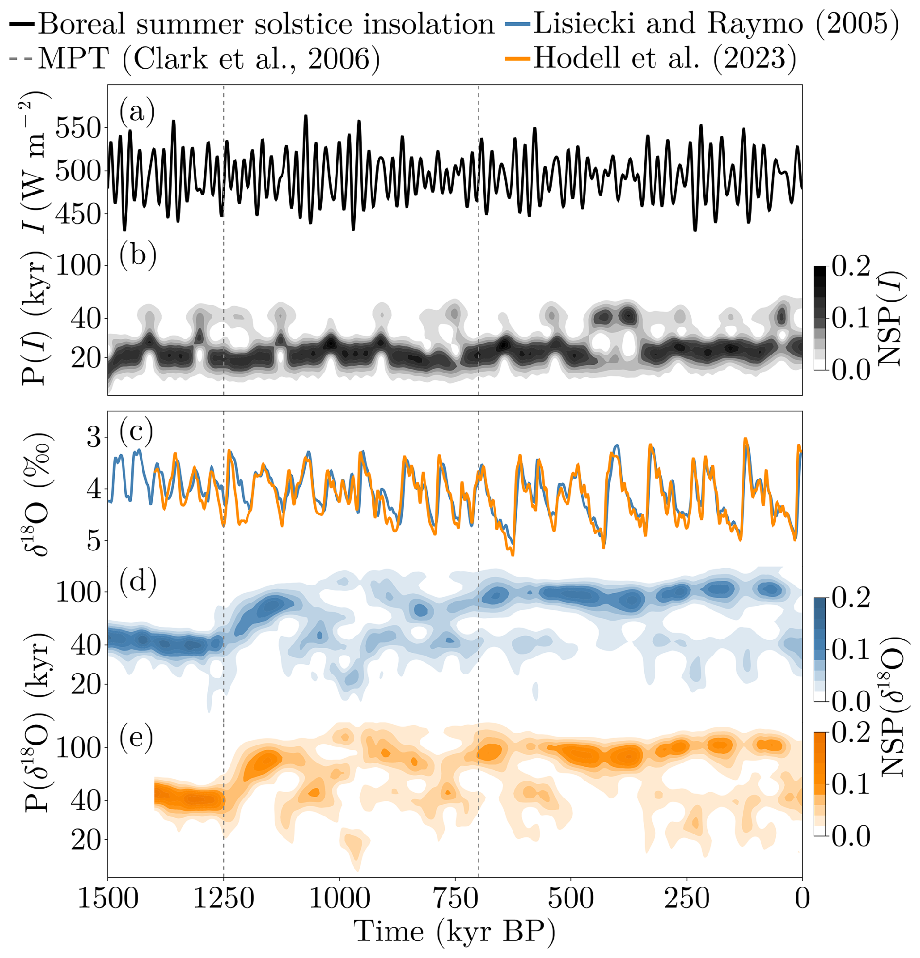
Figure 1 (a) Boreal summer solstice insolation (SSI) at 65° N calculated following Berger (1978) and (b) its wavelet transform. (c) Lisiecki and Raymo (2005, blue) and Hodell et al. (2023, orange) δ¹⁸O time series for the last 1.5 million years and (d, e) their respective wavelet transforms. Note that wavelet transforms in panels (b), (d), (e) show the normalized (integrated) spectral power (NSP) at each period (P) as a function of time. Vertical dashed lines correspond to the interval associated with the occurrence of the MPT (Clark et al., 2006). Proxy records were filtered with a lowpass Butterworth filter (cutoff frequency of 10 kyr⁻¹).

The physical mechanisms behind the MPT are not fully identified. In the past decades various mechanisms invoking ice sheets, sea ice, the ocean circulation and the carbon cycle have been proposed to explain it. The main hypotheses to date are the regolith hypothesis (Pisias and Moore, 1981; Berger and Jansen, 1994; Clark and Pollard, 1998; Clark et al., 2006; Ganopolski and Calov, 2011; Willeit et al., 2019; Carrillo et al., 2024) and the cooling trend in climate conditions (due to the gradual decrease in the atmospheric CO₂ concentration, Raymo et al., 1997; Tziperman and Gildor, 2003; Paillard and Parrenin, 2004; Hodell and Venz-Curtis, 2006; Clark et al., 2006; Verbitsky et al., 2018; Willeit et al., 2019; Carrillo et al., 2024; Clark et al., 2024). The reader is referred to Chalk et al. (2017), Berends et al. (2021a) and Martin et al. (2024) for extensive reviews on this matter.

The regolith hypothesis is based on the existence, at the beginning of the Pleistocene, of a thick layer of unconsolidated sediments (regoliths) formed during the warmer Pliocene epoch (5.33–2.58 million years BP, Setterholm and Morey, 1995; Clark et al., 1999; Goss and Rooney, 2023) that used to cover the continents and that could have affected the dynamics of the ice sheets through enhanced sliding (Fig. 2, Clark and Pollard, 1998; Willeit et al., 2019; Ganopolski, 2024). In this way, at the Early Pleistocene, ice-sheet flow would have been faster, making ice sheets more sensitive to surface mass balance changes produced by relatively small anomalies in incoming solar radiation. However, the basal ice flow gradually advected the sediments outside of the ice sheets, thus thinning the sediment layer and reducing basal velocity. The overall ice flow therefore became slower and less insolation-sensitive, and other processes started to gain importance as triggers of glacial terminations (for a full description of the hypothesis, see Clark et al., 2006). The cooling trend hypotheses are employed by most of the models and are supported to some extent by proxy evidence (and model-assisted proxy evidence, Berends et al., 2021a) that imply a decreasing atmospheric temperature and CO₂ concentration across the Pleistocene due to reduced volcanic outgassing or increased weathering (Clark et al., 2006; Willeit et al., 2019; Berends et al., 2021b). This trend toward a colder climate would in principle facilitate the growing of bigger ice sheets that could have lasted longer in the Late Pleistocene.

Figure 2 (a) Present-day (PD) sediment spatial distribution above PD sea level from Mooney et al. (2023) together with ice sheet extent during the Last Glacial Maximum (LGM, blue colors) from Roy and Peltier (2018, ICE7G) and (grey colors) PD emerged continents outside the maximum extent of the LGM ice sheets. (b) Histograms of sediment thickness in the regions delineated in panel (a).

Pérez-Montero et al. (2025) described the new conceptual model PACCO (Physical Adimensional Climate Cryosphere mOdel) and showed its capability to reproduce the Late-Pleistocene GIV. Experiments with PACCO showed that ice-sheet dynamics, glacial isostatic adjustment and the delayed effect of the ice-sheet thermodynamics on basal sliding lead to slow glaciations and fast glacial terminations of the appropriate amplitude. Together with the darkening of ice through enhanced dust deposition with time, the model produced 100 kyr glacial cycles in agreement with proxies and reconstructions both in timing and in shape. In this work, we will use PACCO to explore the effect of ice velocity on the sensitivity of the Northern Hemisphere ice sheets to climate boundary conditions and its role in relation with the MPT. Thus, we will first focus on the regolith hypothesis. To this end, PACCO is extended to represent sediment layer dynamics. Next, we will analyze how the insolation metric used affects our results. Finally, we will explore the role of trends in the carbon cycle and the hydrological cycle in order to reproduce the MPT.

2 Model description

PACCO represents the interaction between the Northern Hemisphere ice sheets and climate by eliminating the spatial dimensions of ice-sheet dynamics equations and coupling them to a simple climate model that translates insolation forcing (I, only boundary condition) to ice-sheet mass balance (Pérez-Montero et al., 2025). Thus, the prognostic variables of the model are: regional air temperature (T, Appendix A1), CO₂ concentration (C, Appendix A2), ice thickness (H, Appendix A3) and bedrock elevation (B). In the present work, we further include the sediment layer thickness (H_sed), following the scheme in Fig. 3. We describe the governing equation of the sediment layer thickness below and refer to Pérez-Montero et al. (2025) for all processes that are not described here.

Figure 3 PACCO processes flowchart. Note that we highlight in black the new process added to the model and its interaction with the rest of the components.

Adding sediment layer dynamics to PACCO

As described by Pérez-Montero et al. (2025), ice-sheet dynamics are represented by a velocity calculation that accounts for both deformational and sliding regimes in an ice sheet:

$$\begin{array}{}\text{(1)}& v={\displaystyle \frac{\mathrm{2}}{\mathrm{5}}}\cdot A_{\mathrm{f}}\cdot H\cdot {\mathit{\tau }}_{\mathrm{d}}^{\mathrm{3}}+\mathit{\beta }\cdot f_{\text{str}}\cdot C_{\mathrm{s}}\cdot {\mathit{\tau }}_{\mathrm{b}}^{\mathrm{2}},\end{array}$$

where

$$\begin{array}{}\text{(2)}& {\mathit{\tau }}_{\mathrm{d}}={\displaystyle \frac{{\mathit{\rho }}_{\text{ice}}\cdot g}{c}}\cdot {\displaystyle \frac{H}{z}}\end{array}$$

is the driving stress under which gravity deforms the ice, and

$$\begin{array}{}\text{(3)}& {\mathit{\tau }}_{\mathrm{b}}={\mathit{\rho }}_{\text{ice}}\cdot g\cdot H\cdot \mathit{\theta }\end{array}$$

is the basal stress that determines the ice-sheet sliding over the underlying bedrock. In Eqs. (1)–(3) A_f is the Glen's law flow parameter that accounts for ice viscosity (Glen, 1958), f_str is the fraction of ice streams in the ice sheet (Margold et al., 2015), C_s is a sliding parameter derived from Pollard and DeConto (2012), ρ_ice is the ice density, g is the gravitational acceleration, c is the amplitude of the assumed parabolic profile for determining ice deformation (following Verbitsky et al., 2018, see Pérez-Montero et al., 2025) and θ is the slope of the ice-stream region (Benn et al., 2019). H is the ice-sheet thickness, whose evolution is defined in Appendix A3. β is the novelty in the model and it is a fraction between 0 and 1 that represents the potential sliding of the Northern Hemisphere ice sheets defined as:

$$\begin{array}{}\text{(4)}& \mathit{\beta }={\displaystyle \frac{H_{\text{sed}}-H_{\text{sed, min}}}{H_{\text{sed, max}}-H_{\text{sed, min}}}},\end{array}$$

where H_{sed, min}, H_{sed, max} are paleoclimatic constraints on minimum (e.g. present day, PD see Fig. 2) and maximum (e.g. Pliocene, Goldich, 1938; Setterholm and Morey, 1995; Clark et al., 2006) values of sediment layer thickness. β represents the anomaly of sediment coverage with respect to the early Pleistocene and therefore captures how likely it is for the ice sheet to reach sediment-covered areas (based on sediment masks from  Ganopolski and Calov, 2011; Willeit et al., 2019). Of course, the choice of the function shaping β is arbitrary; we selected a linear relationship for the sake of simplicity. However, the versatility of PACCO allows the implementation of more sophisticated relationships. Finally, H_sed evolves in time following:

$$\begin{array}{}\text{(5)}& {\displaystyle \frac{\mathrm{d}{H}_{\text{sed}}}{\mathrm{d}t}}=f_{\dot{p}}\cdot \dot{p}-f_v\cdot v.\end{array}$$

Glen (1958)Verbitsky et al. (2018)Pollard and DeConto (2012)Clark and Pollard (1998)Cuffey and Paterson (2010)Jamieson et al. (2008)Golledge et al. (2013)Cook et al. (2020)Margold et al. (2015)Clark et al. (2006)Benn et al. (2019)

Table 1 Model parameters.

The first term on the right hand side (RHS) represents the denudation rate, which is the process that increases the presence of sediments via weathering (Clark and Pollard, 1998; Cuffey and Paterson, 2010). Thus, $f_{\dot{p}}$ is the fraction of precipitation $\dot{p}$ that produces new sediments (Lebedeva et al., 2010). $\dot{p}$ is equal to snowfall $\dot{s}$ when there is no ice (i.e. H=0, only during interglacials). This choice is motivated by the assumption that during interglacials the climate is warmer and accumulation is given by liquid water instead of snow, thus eroding the rock instead of accumulating snow. The second RHS term is the sediment flux produced by the quarrying of the bed due to the movement of the ice sheet (Jamieson et al., 2008; Golledge et al., 2013; Cook et al., 2020). f_v then represents the proportion of sediments that are eliminated because of the ice-sheet flow. Combining Eqs. (1), (4) and (5), it can be seen that the evolution of H_sed translates into a change in the sliding of the ice sheet thus changing its total velocity.

Finally, z is the ice surface elevation that is defined as

$$\begin{array}{}\text{(6)}& z=H+H_{\text{sed}}+B.\end{array}$$

Including interactive sediments in PACCO results in an additional negative feedback between sediment thickness and ice velocity (Fig. 3), which directly affects the dynamics (Eq. 1) and mass conservation of the ice sheet (Eq. A4). The Appendix A is dedicated to further selected equations, already introduced by Pérez-Montero et al. (2025), which are relevant in the context of the present study.

3 Results

In this section we describe the experiments performed and analyze their main results. To do so, we first show a baseline experiment with the standard model setup that reproduces the entire Pleistocene (Sect. 3.1). Then, we test the sensitivity of PACCO to the parameters of Eq. (5) in Sect. 3.2. Next, an experiment to assess the amplifying role of CO₂ is carried out in Sect. 3.3. Then, we investigate the definition of insolation forcing and its effect on the pre-MPT response in Sect. 3.4. Finally, we test other hypotheses beyond the regoliths in Sect. 3.5. All experiments are summarized in Table 2.

Table 2 Summary of the experiments performed in this work.

3.1 BASE experiment

The BASE experiment (Table 2) is a simulation of the entire Quaternary (from 3 Myr BP to present) obtained by forcing PACCO with the boreal summer solstice insolation (SSI) at 65° N following Berger (1978). The values of the parameters and initial conditions can be found in Tables 1 and A1. We use a model configuration that includes ice-sheet dynamics, isostasy, carbon cycle and albedo darkening (i.e. the AGING configuration in Pérez-Montero et al., 2025). By including the basal sliding dependence on the interactive sediment evolution we obtain good qualitative agreement between simulation results and proxies, including a change in the periodicity of the system around 1250–700 kyr BP, the MPT.

As can be seen in Fig. 4, the GIV in BASE is generally in good agreement with proxies, especially the sea-level evolution over the last 800 kyr. Before the MPT, the ice volume presents a slightly lower amplitude than the one suggested in proxies. This is due to the geometric assumption of a circular ice domain that underlies the computation of spatially averaged quantities (Eq. A8), which does not capture the spatial heterogeneity of the regolith-cleared areas. Note that the work of Clark et al. (2025) is the first ice volume reconstruction that shows a constant amplitude of ice volume throughout the entire Pleistocene. This particular finding will be discussed in Sect. 4. Most importantly, BASE displays a change in both amplitude and periodicity at the MPT. This change is caused by the gradual decrease of the sediment thickness (second term of the RHS of Eq. 5), that decreases the ice velocity (Eqs. 1 and 4) and ultimately increases the ice thickness through Eq. (A4) (Fig. 5). Before the MPT, the ice-volume cycles are faster and smaller since the sediment thickness is higher (Fig. 4f) and the ice-sheet flow is generally faster (Figs. 5b and 6c). Thus, the ice sheet is more sensitive to precession and obliquity periods, which leads to smaller circular trajectories when projecting the phase space onto the insolation and ice-thickness dimensions (Fig. 6b). After the MPT, the gradual reduction in the sediment thickness results in slower ice sheets (Fig. 6c). Therefore, ice sheets grow further, which allows them to persist over several obliquity cycles. As a consequence, glacial cycles last longer compared to the Early Pleistocene (Figs. 5c and 6b). This is reflected in the wavelet transform of the simulated and reconstructed ice volume (Fig. 7). The power spectrum is concentrated around 20–40 kyr before the MPT and around 80–120 kyr after. Hence, compared with proxy records, lower pre-MPT periodicities are obtained. This could be due to the fact that the SSI we use shows a high precessional spectral power (Leloup and Paillard, 2022).

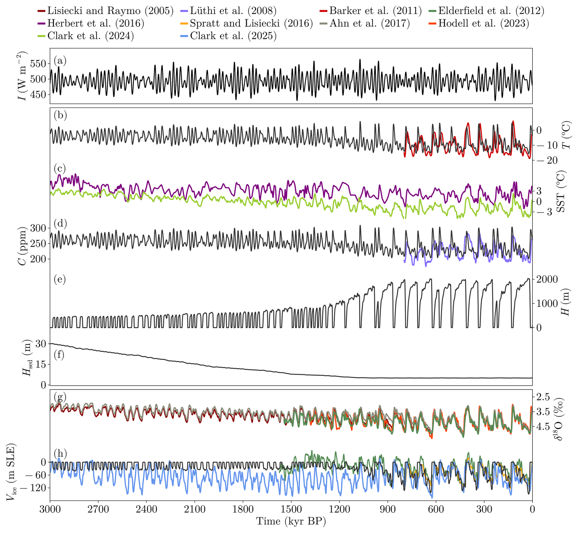
Figure 4 Results of BASE experiment: (a) Boreal SSI, (b) regional air temperature anomaly with respect to T_ref in comparison with Barker et al. (2011), (c) global-mean sea-surface temperature (SST) from Herbert et al. (2016) and Clark et al. (2024). (d) CO₂ concentration compared with Lüthi et al. (2008), (e) ice thickness, (f) sediments thickness, (g) δ¹⁸O from Lisiecki and Raymo (2005), Elderfield et al. (2012), Ahn et al. (2017) and Hodell et al. (2023), and (h) ice volume time series in comparison with Elderfield et al. (2012), Spratt and Lisiecki (2016) and Clark et al. (2025). Note that black curves all represent results simulated with PACCO.

Figure 5 (a) Results from the BASE experiment showing the evolution of the ice thickness H (in gray) and mass balance terms (snowfall $\dot{s}$, ablation $\dot{a}$ and ice discharge q normalized by $\dot{s}$, as defined in Appendix A3) for different ranges of time: (b) pre-MPT world and (c) post-MPT world.

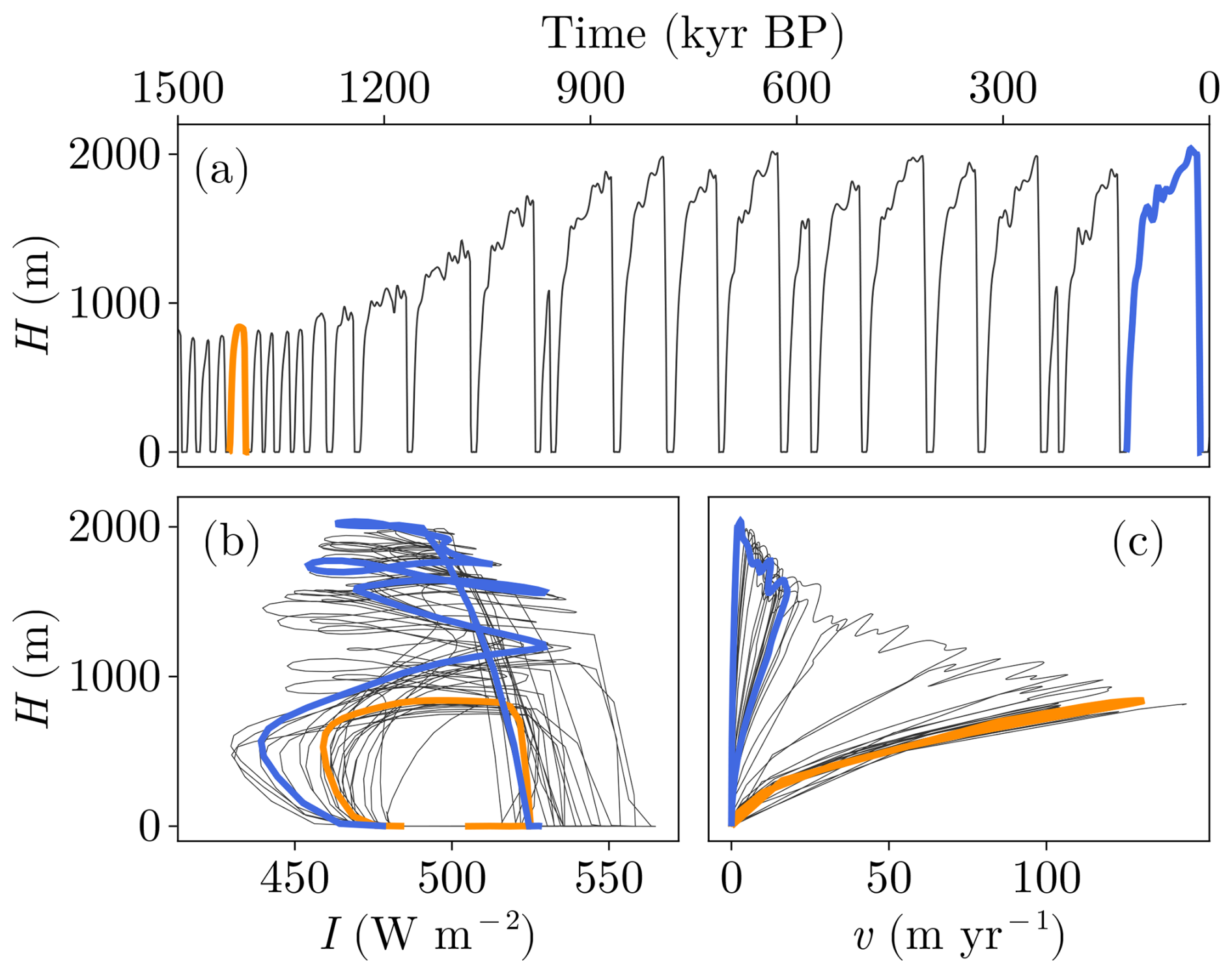
Figure 6 (a) Ice thickness time series from BASE experiment. (b, c) Ice thickness trajectories from BASE experiment as a function of insolation forcing and ice sheet velocity. Note that we have highlighted two cycles of 40 and 100 kyr respectively in orange and blue.

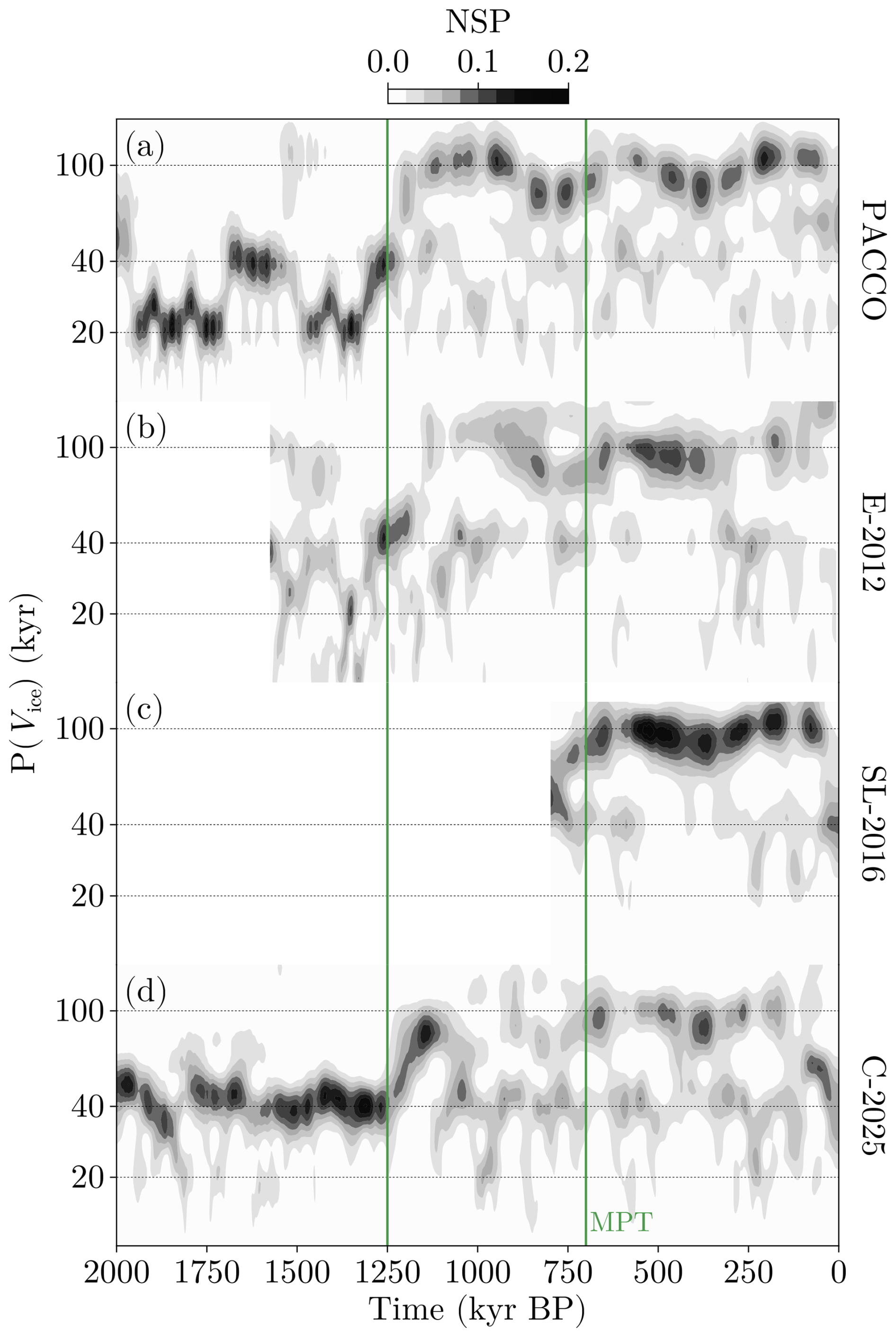
Figure 7 NSP of ice volume V_ice at each period (P) as a function of time from (a) BASE experiment, (b) Elderfield et al. (2012, E-2012), (c) Spratt and Lisiecki (2016, SL-2016) and (d) Clark et al. (2025, C-2025). Vertical green lines correspond to the interval associated with the occurrence of the MPT (Clark et al., 2006).

As introduced in Sect. 1, the MPT has been suggested to occur because of the decreasing trend in CO₂ or temperature. In our model, introducing ad-hoc temperature or CO₂ trends is not needed since they are produced naturally by the model via the cooling effect of the gradually thicker ice sheets throughout the Pleistocene (c_z⋅z in Eq. A1). The modulation of the ice-surface elevation z via basal dynamics provides us with such trends in climate. Thus, these trends in PACCO are consequences rather than triggers of the MPT.

As we described above, the gradual reduction of the sediment thickness plays a key role in producing an MPT that is coherent with proxy records. We therefore propose to study the sensitivity of the results to the parameters controlling the evolution of H_sed.

3.2 Sensitivity to sediment evolution (SEDIM experiment)

In Eq. (5) we use two parameters, the denudation and quarrying fractions ($f_{\dot{p}}$ and f_v, respectively) to represent a rather complex process in a simple manner. Thus, we perform a sensitivity experiment (SEDIM, Table 2) to investigate the effect of the values of these parameters selected in BASE. Golledge et al. (2013) propose ${\mathrm{10}}^{-\mathrm{6}}\mathrm{m}{\mathrm{yr}}^{-\mathrm{1}}$ as a reasonable value for the quarrying fraction f_v. They found values of sediment fluxes ranging from 100 to more than 1000 m³ yr⁻¹, which corresponds to $f_v\in [{\mathrm{10}}^{-\mathrm{8}},{\mathrm{10}}^{-\mathrm{6}}]$ for a typical ice sheet area (L²) of about 10¹⁰−10¹² m². Moreover, the denudation fraction $f_{\dot{p}}$ is estimated to be about ${\mathrm{10}}^{-\mathrm{6}}-{\mathrm{10}}^{-\mathrm{5}}\mathrm{m}{\mathrm{yr}}^{-\mathrm{1}}$ in west Greenland (Strunk et al., 2017) during the last 1 million years, $\mathrm{1.5}\times {\mathrm{10}}^{-\mathrm{5}}\mathrm{m}{\mathrm{yr}}^{-\mathrm{1}}$ in the Svalbard archipelago during the Holocene (Svendsen et al., 1989), and up to ${\mathrm{10}}^{-\mathrm{3}}\mathrm{m}{\mathrm{yr}}^{-\mathrm{1}}$ in the Alps (Delunel et al., 2020). These two parameters control the time when the MPT occurs, as shown in Fig. 8, defined as

$$\begin{array}{}\text{(7)}& t_{\text{MPT}}=t(H_{\text{sed}}=\mathrm{6}),\end{array}$$

since we empirically observed a threshold in the oscillatory regime around that value of sediment thickness. Figure 8 shows two regimes: If $f_{\dot{p}}$ is below 10⁻⁵, f_v dictates the timing of MPT (ice dynamic regime). Above 10⁻⁵, $f_{\dot{p}}$ becomes important (precipitation regime). This highlights the fact that, as long as the weathering fraction partially equilibrates the quarrying fraction, the run transitions from one regime to the other with the right timing (i.e. during the MPT period observed in the proxies, Clark et al., 2006). This is represented by Fig. 9, which shows the evolution of H and H_sed fixing one parameter and changing the other one around the BASE case. Depending on the value of $f_{\dot{p}}$, interglacials generate more or less sediments to the point of overweighting sediment removal. Something similar occurs when fixing $f_{\dot{p}}$, but in this case, if $f_v\le f_{\dot{p}}$, we can achieve the right timing of the MPT. Finally, as shown in Fig. 8, BASE displays a correct timing of the MPT which can however be also obtained with other parameter combinations.

Figure 8 MPT onset (t_MPT) for an ensemble of 9240 evenly spaced permutations of f_v and $f_{\dot{p}}$ (Note that the BASE experiment is represented by the big black dot). Green colors show transitions that start between 1250 and 700 kyr BP (Clark et al., 2006) and the gray zone represents the runs in which the sediment thickness shows an increasing rather than a decreasing trend. Finally, black dashed lines correspond to the curves shown in Fig. 9.

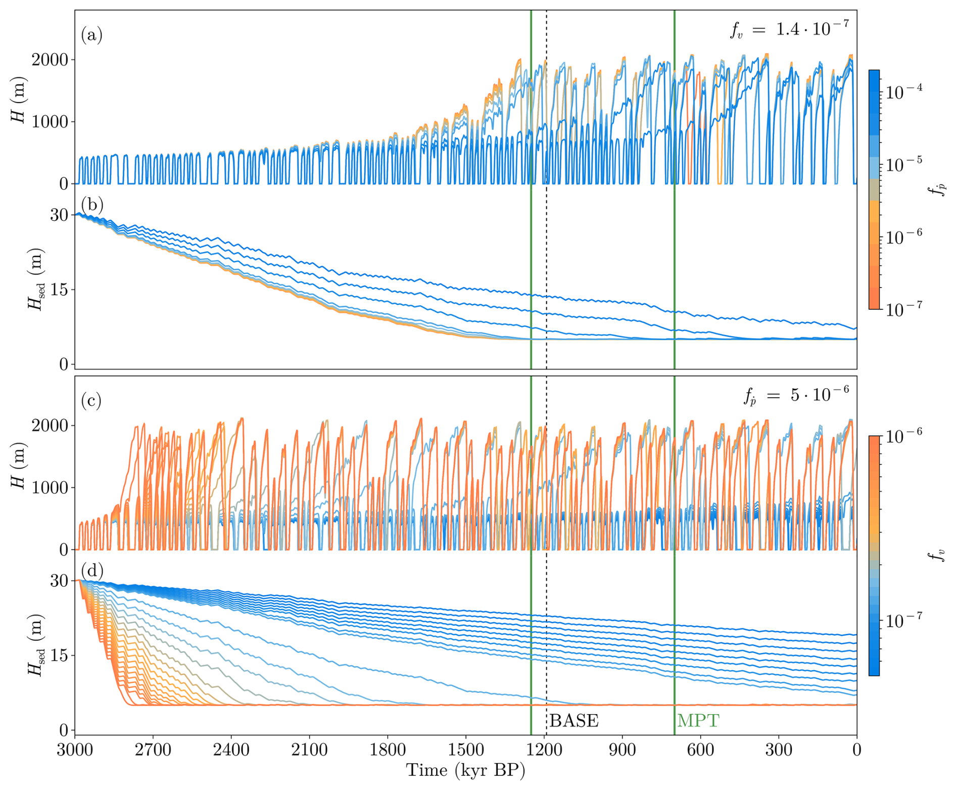
Figure 9 Time series for two experiments varying (a, b) $f_{\dot{p}}$ and (c, d) f_v only, respectively. Note that the vertical green lines indicate the bounds of the MPT as found in the proxies (Clark et al., 2006) and the dashed black and vertical line the MPT as obtained in the BASE experiment. Note that we have removed the series whose sediments increase rather than decrease throughout the entire series since their parameter space is not coherent with the paleoclimatic constraints. For clarity we have only plotted every 5th simulation of the ensemble.

Of course, the particular calibration of the run can in principle alter Fig. 8. However, for a fixed parameter space, the selection of $f_{\dot{p}}$ and f_v depends on the partial balance between both contributions, which results in the regimes described above (ice and precipitation regimes).

3.3 The amplifying effect of CO₂ (CARBON experiment)

Previous work (e.g., Ganopolski and Calov, 2011; Willeit et al., 2019) has analyzed the role of CO₂ in GIV, concluding that its variability is not as important as its average background value. To verify this in PACCO, we turn off the carbon cycle component and perform a series of experiments where we apply a constant level of atmospheric CO₂. Otherwise, the rest of the parameters are the same as in BASE. The results for several atmospheric CO₂ levels are presented in Fig. 10. In PACCO, CO₂ shows the same amplifying role as in the aforementioned studies. Since CO₂ affects temperature, accumulation changes and the cycles decrease their amplitudes depending on the level of this gas. During the pre-MPT world, the median of the temperature distribution in each run increases with the imposed background atmospheric CO₂ level (Fig. 10h–l). However, the median temperature of the post-MPT world is nearly the same except for the highest atmospheric CO₂ level inspected, 380 ppm. The climate in this run is especially warm. Accordingly, ablation is greatly favored, making the denudation term in Eq. (5) greater than the quarrying one for the entire Pleistocene. Thus, the transition does not occur (Fig. 10b). For atmospheric CO₂ levels in the range of 100–300 ppm, the model always transitions to the post-MPT world. Runs using atmospheric CO₂ levels between 200–300 ppm are similar to BASE. In contrast, the 100 ppm runs show longer cycles before the MPT. The climate is cold enough to largely inhibit thermal ablation and allow for larger pre-MPT ice sheets that do not experience deglaciation at each obliquity cycle.

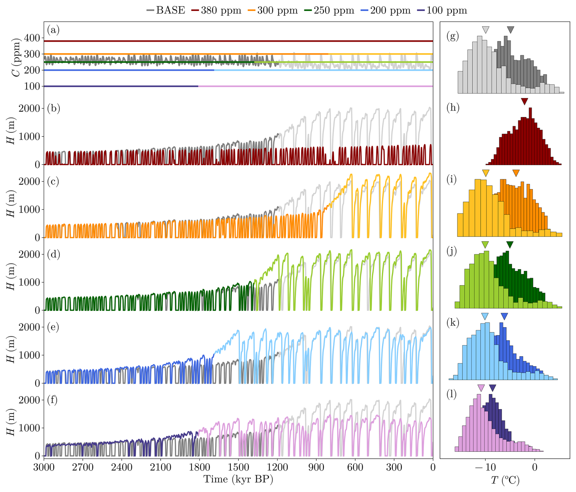
Figure 10 (a) Time series of C for each run. Note that darker colors indicate the pre-MPT world (H_sed>6 m) and lighter colors in the post-MPT world. (b–f) Time series of H for each CARBON run and BASE as a reference. (g–l) Histograms (normalized as probability density functions) of T for each CARBON run (h–l) and BASE (g). Note that the inverted triangles point to the median of each distribution.

In summary, this experiment shows that the interactive carbon cycle in PACCO is an amplifier of GIV rather than the trigger of MPT, in accordance with previous literature results. This finding relies on the fact that the change in regime in PACCO is due to purely dynamic reasons. In our case, the MPT does not need a trend in climate (via CO₂ or temperature) since it is produced naturally by the effect of ice sheets on climate.

3.4 Insolation forcing definition (INSOL experiment)

In Sect. 3.1 we have seen that the pre-MPT world in PACCO has too much spectral power in the 20 kyr band to be fully coherent with proxy records. In this section we will investigate the effect of the definition of the insolation forcing in this result. Leloup and Paillard (2022) compared the three common definitions of insolation forcing applied in conceptual modeling oriented to orbital-scale variability studies and discussed the relative spectral power of each orbital parameter and their effect on glacier ablation; for a complete description of these metrics see Leloup and Paillard (2022), Tzedakis et al. (2017), Huybers (2006) and Milankovitch (1941). We define the summer solstice insolation (SSI), the integrated summer insolation (ISI) and the caloric season insolation (CSI) following the previous cited studies as:

$$\begin{array}{}\text{(8)}& {\displaystyle }& {\displaystyle }\text{SSI}\left(t\right)=I(t,\mathrm{170},\mathrm{65}),\text{(9)}& {\displaystyle }& {\displaystyle }\text{ISI}(t,I_{\text{thr}})=\sum _{i=\mathrm{1}}^l{w}_i\cdot I(t,i,\mathrm{65}),\text{(10)}& {\displaystyle }& {\displaystyle }\text{CSI}\left(t\right)=\sum _{i=\mathrm{1}}^l{w}_i^{\prime }\cdot I(t,i,\mathrm{65}).\end{array}$$

$I=(t,d,\mathit{\varphi })$ depends on the time (t), the day (d) and on the latitude (ϕ) in which we compute insolation following Berger (1978). The weight w_i yields 1 if $I(t,i,\mathrm{65})\ge I_{\text{thr}}$ and 0 otherwise. In contrast, the weight $w_i^{\prime }$ yields 1 if $I(t,i,\mathrm{65})$ is above the median of the year's distribution and 0 otherwise. ISI and CSI are therefore computed as weighted integration of I, with l the summation index that represents the length of the year in days. Note that SSI has units of W m⁻² and ISI and CSI of J m⁻² (Fig. B1).

We performed three experiments: BASE (that uses SSI), CSI and ISIn (n indicates the insolation threshold applied to ISI metric). The results are plotted in Fig. 11 using insolation thresholds of 0, 275, 300 and 400 W m⁻² (i.e., ISI275, ISI300 and ISI400, respectively). These selections were made following Huybers (2006, ISI275) and Leloup and Paillard (2022, ISI300 and ISI400). ISI0 was performed as a contrasting case in which we included the full annual integrated insolation.

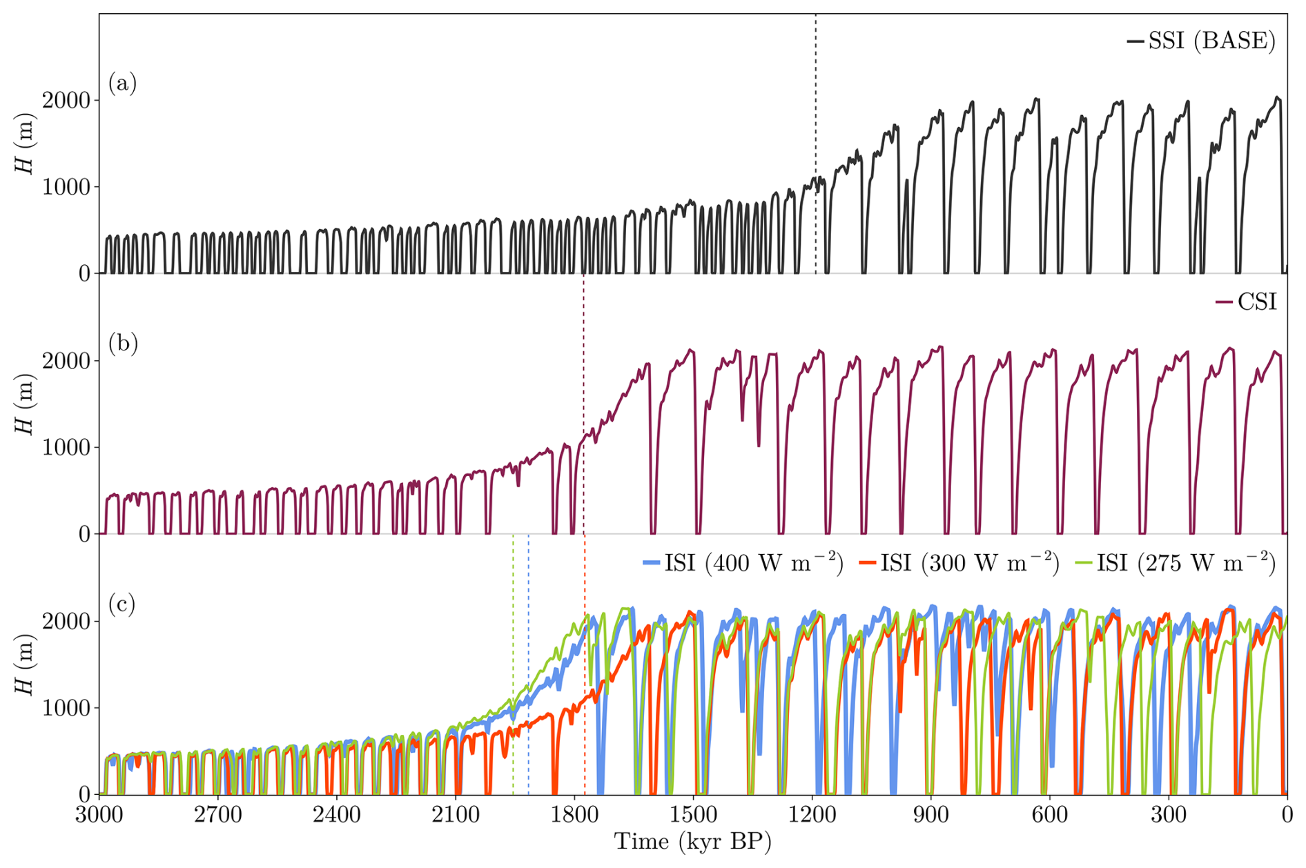
Figure 11 Time series of ice sheet volume for the different insolation metrics: (a) summer solstice insolation, (b) caloric season insolation and (c) integrated summer insolation using $I_{\text{thr}}=[\mathrm{275},\mathrm{300},\mathrm{400}]\mathrm{W}{\mathrm{m}}^{-\mathrm{2}}$. Please note that we have only changed the sensitivity to insolation parameters (Table 1), so the MPT occurs at different times in each simulation. Vertical dashed lines indicate the MPT as defined in the previous section for each run.

After calibrating the insolation sensitivities (c_I and k_I in Eqs. A1 and A7) to account for the fact that in PACCO insolation is expressed as energy and not power, we obtain similar curves to the BASE run. This is particularly the case for the post-MPT world, as shown in Fig. 11. During the late Pleistocene all series share a similar power spectral density (Fig. 12c), indicating that the particular definition of the forcing is not a decisive factor for the post-MPT world. However, in the pre-MPT world, the spectral power in the CSI and ISIn experiments is located around 40 kyr. This finding is related to the spectral power of each Milankovitch period in these metrics (Fig. 12a). CSI and ISI metrics yield more 40 kyr power since precessional power is eliminated in favor of obliquity when integrating in time (Leloup and Paillard, 2022). In addition, these metrics indirectly alter the capability of the ice sheet to remove sediments since the pre-MPT cycles are longer (compared to BASE) and thus eliminate sediments quickly. For this reason, MPT occurs earlier in CSI and ISIn (Fig. 11).

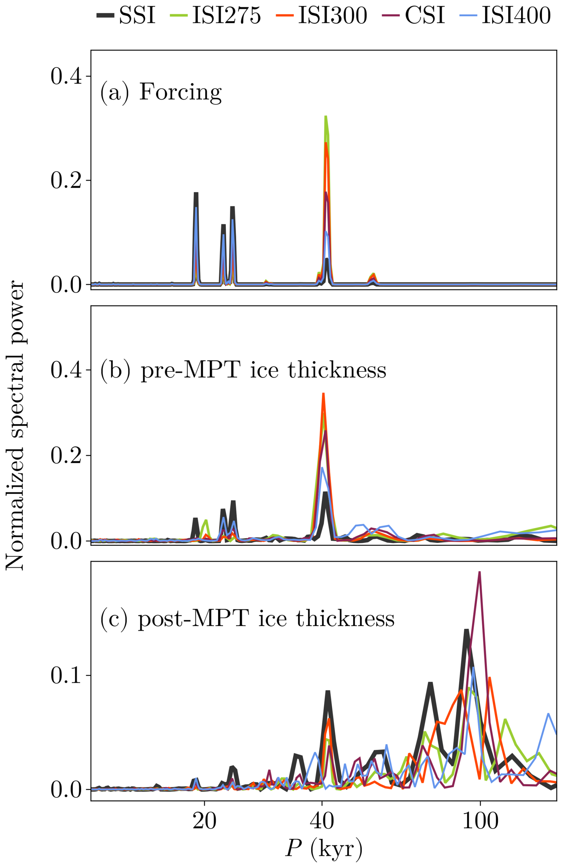
Figure 12 Normalized spectral power of (a) insolation forcing, (b) pre-MPT and (c) post-MPT ice thickness corresponding to each forcing in the INSOL experiment.

Therefore, we conclude that there is an improvement in the pre-MPT world in terms of the simulated periodicity, but not in terms of the amplitude when using CSI or ISI metrics. Thus, for historical reasons (Paillard, 1998; Parrenin and Paillard, 2003; Leloup and Paillard, 2022; Ganopolski, 2024), to reduce the computational cost and to allow for a more direct comparison of the role of different mechanisms (Raymo and Nisancioglu, 2003; Raymo et al., 2006) we continue in the following sections to use SSI as the model forcing. This improvement does not alter our main finding on the important role of regolith quarrying to trigger the MPT, in contrast with decreasing trends in temperature and CO₂, which occur as consequences of changes in the cryosphere in this model.

3.5 Exploring hypotheses beyond the regoliths

BASE results fundamentally rely in the dynamic change of the sediment layer thickness. Thus, a plausible question is: What would happen to our results if we do not consider the sediment layer evolution? In other words, what if the regoliths formed during the Pliocene were removed from the continents long before the MPT? To this end, we performed two experiments deactivating the sediment layer dynamics: NOSEDIM-high and NOSEDIM-low (Table 2 and Fig. 13). These experiments present the same model setup as the AGING configuration in Sect. 2.7 from Pérez-Montero et al. (2025). The only difference is that we started them at 3 Myr BP and applied two different basal sliding parameter values: $C_{\mathrm{s}}=\mathrm{6}\times {\mathrm{10}}^{-\mathrm{5}}\mathrm{m}{\mathrm{yr}}^{-\mathrm{1}}{\mathrm{Pa}}^{-\mathrm{2}}$ for NOSEDIM-high (the same as BASE) and $C_{\mathrm{s}}=\mathrm{3}\times {\mathrm{10}}^{-\mathrm{8}}\mathrm{m}{\mathrm{yr}}^{-\mathrm{1}}{\mathrm{Pa}}^{-\mathrm{2}}$ for NOSEDIM-low (the same value as in Pérez-Montero et al., 2025). As can be seen in Fig. 13, during NOSEDIM experiments, the model does not transition from the pre- to the post-MPT worlds. Instead, the model remains in the dynamic regime determined by the imposed sliding intensity: 20–40 kyr world with high sliding and 80–120 kyr world with low sliding. This fact was expected since there is no change in the system behavior that alters the mass balance of the ice sheet. In this context, we will analyze the effect of introducing a cooling trend in the climate and whether that trend is capable of altering the mass balance of the ice sheets sufficiently to provide a change in the system periodicity when sliding is not interactive with basal sediment thickness.

Figure 13 Time series of (a) ice thickness H and (b) total velocity v for BASE and NOSEDIM-high ($C_{\mathrm{s}}=\mathrm{6}\times {\mathrm{10}}^{-\mathrm{5}}\mathrm{m}{\mathrm{yr}}^{-\mathrm{1}}{\mathrm{Pa}}^{-\mathrm{2}}$, orange) and NOSEDIM-low ($C_{\mathrm{s}}=\mathrm{3}\times {\mathrm{10}}^{-\mathrm{8}}\mathrm{m}{\mathrm{yr}}^{-\mathrm{1}}{\mathrm{Pa}}^{-\mathrm{2}}$, blue).

3.5.1 The cooling effect of a trended carbon cycle

In Sect. 1 we noted that many studies contemplate the MPT as the consequence of a cooling trend in climate. Figure 14 shows the effect of adding this trend to the NOSEDIM-low experiment. As can be seen, the trend in C allows much higher accumulation rates in the Early Pleistocene, producing higher amplitudes of H relative to Late Pleistocene. This effect increases monotonically with the trend applied until a threshold is reached (orange to red colors in Fig. 14a) and the ablation surpasses accumulation, inhibiting glacial inception (Fig. 14c). Again, we can see that the carbon cycle in PACCO only affects the amplitude of GIV and has little influence on the periodicities except for the cases in which CO₂ is sufficiently (and probably unrealistically) high at the Early Pleistocene. In fact, applying the same experiment to NOSEDIM-high (not shown) shows the same behavior. At this point, one could ask: if the carbon cycle just amplifies the amplitude of GIV, did other climate-related processes significantly change during the Pleistocene, allowing the observed ice-volume variation in proxies? We will answer that question in the following section.

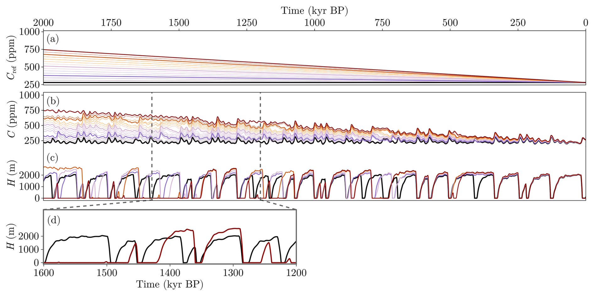
Figure 14 Time series of (colors) TREND-C experiment and (black) NOSEDIM-low experiment. (a) Reference carbon dioxide C_ref, (b) carbon dioxide C, (c) ice thickness H and (d) zoom of the range squared in panel (c) for the two extreme cases. Note that in panel (c) only the curves highlighted in panels (a) and (b) are plotted.

3.5.2 What if the hydrological cycle changes over time?

The classical interpretation of δ¹⁸O implies lower ice-sheet volumes during the Early Pleistocene. In the previous section we have seen that in our results, the carbon cycle mainly modifies the amplitude rather than facilitating any change in the periodicities of the glacial cycles. It is, however, plausible that climate sensitivity (in its broad sense) had changed during the Pleistocene. Thus, here we wonder about the effects that, for instance, a variable hydrological cycle could have on the MPT. To answer that question we performed an experiment applying a trend to the sensitivity of snowfall accumulation to temperature $k_{\dot{s}}$ (Appendix A3, Eq. A6) to NOSEDIM-low (Fig. 15). As can be seen, increasing $k_{\dot{s}}$ allows a change in the GIV regime across the Pleistocene (Fig. 15d). This change comes from the fact that if a higher accumulation sensitivity to temperature is allowed, the ice sheet is more reactive to changes in its mass balance. Thus, at the Early Pleistocene, the ice sheet evolves more strongly with insolation forcing for a certain level of $k_{\dot{s}}$. After several hundred of thousand of years, that sensitivity is reduced and the solution converges to NOSEDIM-low and hence to the Late Pleistocene simulated in BASE.

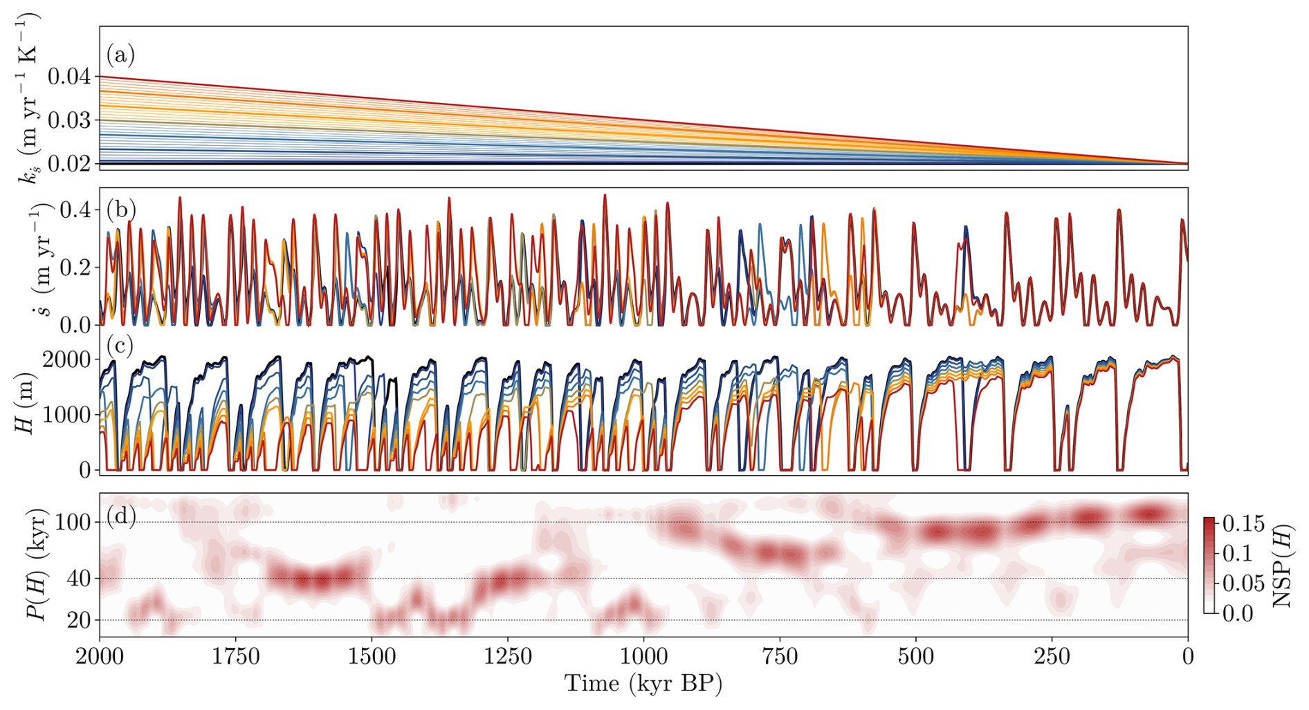
Figure 15 Time series of (colors) TREND-S experiment and (black) NOSEDIM-low experiment. (a) Sensitivity of accumulation to temperature $k_{\dot{s}}$, (b) snowfall $\dot{s}$, (c) ice thickness H and (d) wavelet transform of H for the maximum decreasing trend (red) case. Note that in panels (b) and (c) only the curves highlighted in panel (a) are plotted.

In summary, although imposing an ad-hoc decreasing trend in CO₂ does not produce an MPT in our model, we show that a progressive reduction of the sensitivity of precipitation to temperature does facilitate the shift in periodicities observed during the MPT. This indicates that perhaps the MPT could have been triggered or facilitated by another climate subsystem that influences the hydrological cycle sensitivity (e.g., the precipitation patterns, Gildor and Tziperman, 2001).

4 Discussion

4.1 Role of the regolith layer and limitations in our approach

In this work we have simulated the entire Pleistocene with the spatially adimensional and conceptual climate-cryosphere model PACCO (Pérez-Montero et al., 2025). To this end, we have added a new process to the original model that accounts for the existence of a dynamic and soft sediment layer beneath the Northern Hemisphere ice sheets. This hypothesis is based on the evidence of remnants of these layers over the Northern Hemisphere continents (Fig. 2, Pisias and Moore, 1981; Berger and Jansen, 1994; Clark and Pollard, 1998; Clark et al., 2006; Ganopolski and Calov, 2011; Willeit et al., 2019; Carrillo et al., 2024). The weak regolith substratum facilitates glacier basal sliding thus enhancing ice discharge. This mechanism is self-limited since ice flow partially removes the sediments during glacial stages, thus reducing basal sliding and therefore the ice flow. The sediment is only partially regenerated during the comparatively short interglacials. PACCO captures these processes through the representation of the hypothetical imbalance between sediment flux and denudation rate that created the current distribution of sediments along the continents (Fig. 2). This imbalance produces two different dynamic regimes along the Pleistocene. At the early Pleistocene, high levels of sediments allow higher levels of ice discharge that facilitate a full deglaciation via an increase in insolation due to precession and obliquity cycles (Fig. 5b). Subsequently, levels of sediments are lower and thus, ice sheets grow bigger and persist longer. At this point, deglaciations are triggered by the manifestation of different nonlinear processes, among which the albedo darkening facilitates simulating the right timing (Fig. 5c, Pérez-Montero et al., 2025). Therefore, under this simple but physical formulation, the potential sliding of the Northern Hemisphere ice sheets, modulated by the basal dynamics, plays a main role in triggering the MPT and produces the observed trend in climate proxies due to the cooling effect of larger ice sheets in the Northern Hemisphere. These conclusions agree with previous conceptual efforts such as Verbitsky et al. (2018), in which the authors conclude that the simulated MPT is the product of a change in the balance of feedbacks in the system. In a complementary study, Ganopolski (2024) summarized the relevant processes affecting the MPT and included a change in the dynamic regime of the ice sheets and their size as a critical threshold. Willeit et al. (2019) also showed that the regolith removal could have changed the dynamic properties of the Northern Hemisphere ice sheets, propitiating a periodicity regime shift in their Earth System model. Recent studies have also come to different conclusions. For example, (Scherrenberg et al., 2025) concluded that CO₂ variations were vital to producing glacial–interglacial variability. However, in our view, their climate forcing index, based on both insolation and CO₂ proxies, is what induces such a variability in their approach. In contrast, PACCO only includes one boundary condition, which is insolation.

Nonetheless, we must also highlight the implicit limitations of our approach. Since we do not take into account spatial heterogeneity in sediment distribution, some magnitudes may be overestimated (such as total ice-sheet velocity) or underestimated (such as ice volume). In the latter case, on one hand, Eq. (A8) relies on a simplistic geometric assumption. Thus, it does not take into account that certain regions are cleared of sediment and, therefore some ice grows on hard bedrock. Moving more slowly with greater ice volumes. On the other hand, the election of the insolation forcing metric may have and effect on the pre-MPT world, either because of the asymmetry of precession between high latitudes in both hemispheres (Raymo et al., 2006) or because the SSI produces an enhanced response around 20 kyr periodicity preventing the ice sheet to further expand (or gain mass) during longer obliquity-paced cycles (Leloup and Paillard, 2022). However, elucidating the exact cause of the obliquity vs. precession pre-MPT ice-volume amplitude issue is out of the scope of this paper. To resolve this, a three-dimensional ice-sheet model should be used in conjunction with a fully operational sediment flux module; however, to our knowledge, no such approach exists to date. This fact leaves room for possible future work.

4.2 Regolith layer evolution equation

The phase space of the sediment layer equation has been tested for a wide range of the parameters involved in the SEDIM experiment. The imbalance between the quarrying (f_v) and denudation ($f_{\dot{p}}$) fractions defines the rate at which sediments are removed beneath the ice sheets. Therefore, it determines the timing of where the change of dynamic regime. There is no reason for this relationship to be linear and we do not exclude the existence of better representations of the sediment quarrying and generation. However, Eqs. (4) and (5) are enough to show that a gradual, interactive change in the dynamic regime can, in principle, alter the response of the climate system to insolation forcing along the Pleistocene, in agreement with Legrain et al. (2023).

4.3 Carbon cycle

In addition, the role of CO₂ as the GIV amplifier has been explored. Our model reproduces GIV for constant levels of C as long as the prescribed background level remains low enough. The CARBON experiment conclusions align with previous work since it is the average value rather than its fluctuations that allows and amplifies GIV in PACCO (Abe-Ouchi et al., 2013; Willeit et al., 2019). This finding implies that in our work, the trend in CO₂ throughout the Pleistocene can be explained as a consequence of the increased ice-sheet size due to slowing ice dynamics. However, this fact should not necessarily be interpreted as the definitive mechanism leading to the atmospheric CO₂ trend shown by proxies and reconstructions during earlier epochs (Van de Wal et al., 2011; Willeit et al., 2015).

4.4 Insolation metrics

We have also seen that the selection of the particular metric for insolation forcing facilitates the pre-MPT world to oscillate at 40 kyr. Thus, one could see this as a simple forcing choice problem, but it could also hide the role of the Antarctic ice sheet, the pole antisymmetry of precession cycles or the latitudinal insolation gradient (Raymo and Nisancioglu, 2003; Raymo et al., 2006). Still, metric selection or uncertainty about the pre-MPT world does not have any imprint on the simulated post-MPT world, neither with respect to sea-level amplitude nor for their frequencies. This is due to the fact that, once regoliths are depleted enough for the basal sliding to be significantly reduced, the system locks at 100 kyr periodicities regardless of its pre-MPT amplitude. However, the ice volume amplitude of the pre-MPT cycles does slightly influence the timing of the transition. Variations in the pre-MPT amplitudes or frequencies with respect to BASE require a small recalibration of the parameters in sediment dynamics in order to simulate the MPT at the precise timing.

4.5 Role of trends in PACCO's climate

Finally, we tested the role of a cooling trend in climate by separately applying trends in the carbon cycle (Sect. 3.5.1, TREND-C) and in snowfall accumulation (Sect. 3.5.2, TREND-S). Again, we have seen that a trend in PACCO's carbon cycle only amplifies GIV but it does not produce a change in its frequency. This can be a limitation of our adimensional approach as compared to similar modeling efforts such as Willeit et al. (2019). It is conceivable that under high CO₂ atmospheric concentrations a global model such as CLIMBER-2 (Willeit et al., 2019) will inhibit glacial inception in continental areas where ablation remains high, even under cold orbits, so that those glacial maxima will show a relatively low amplitude. In our case, however, due to the lack of spatial dimensions, if those same cold orbits allow for inception, ice sheets will grow according to the mean conditions without reflecting any spatial heterogeneity.

However, as shown in Fig. 15, a trend in snowfall is capable of producing a change of periodicity along the Pleistocene. In this case, we modify directly the mass balance using snowfall sensitivity to temperature as another forcing. Where does this extra forcing come from? We cannot identify the physical mechanism underlying the change in snowfall sensitivity to temperature because of the simplicity of its implementation. However, one could hypothesize possible mechanisms that could imply such a change: In a warmer climate, the hydrological cycle is amplified, thus being more sensitive to changes in short-scale fluctuations of temperature. Then, if air temperature (governed in these timescales by solar radiation) changes, the mass balance of the ice sheet can be affected more strongly. However, in a colder climate, the hydrological cycle is weakened and less sensitive to orbital fluctuations. Thus, we hypothesize here that considering the sea-level reconstruction from Clark et al. (2025), a possible solution would be to take into account the effect of a progressive change in the hydrological sensitivity through the MPT.

The present work shows that the regolith hypothesis can produce a quantitative match of the CO₂ and temperature proxies, which were used to formulate the competing hypothesis of a cooling climate as the main trigger of the MPT. Although this does not discard other mechanisms that could have cooled the climate, it shows that the regolith hypothesis mechanistically explains the cooling and is coherent with proxy records, while being supported by the current sediment distribution at high northern latitudes. In comparison, the cooling climate hypothesis suffers a lack of mechanistic explanation to date, as weathering was likely low since the climate was relatively cold and dry. Additionally, no major change in tectonic or biological processes happened over this time, potentially discarding them as carbon sinks. Of course, it is difficult to come to a final conclusion without proxies with a more accurate time resolution covering the Early Pleistocene.

4.6 A constant ice volume amplitude during the Pleistocene?

Lastly, we see the necessity to point out that the recent study by Clark et al. (2025) ruled out the regolith hypothesis proposed by Clark and Pollard (1998). This study claims that the relative importance of temperature and ice volume in the signal of δ¹⁸O could have changed over the Pleistocene, thus invalidating the assumption of a change in ice volume during the MPT (Fig. 4h). However, in our view, their conclusions remain to be tested in relation with evidence from other reconstructions of the Pleistocene (e.g. ice rafted detritus and other marine sediments, Raymo et al., 1989; Clark et al., 2006; Hodell et al., 2008; Sosdian and Rosenthal, 2009; Rohling et al., 2014; Hodell and Channell, 2016). When comparing both the Pleistocene SSTs (Clark et al., 2024) and the ice volume reconstruction (Clark et al., 2025) an intriguing pattern emerges: pre-MPT and post-MPT glacial maxima appear to have similar sea-level amplitudes while global pre-MPT SSTs are significantly higher than post-MPT ones. How to build glacial pre-MPT Earth's ice sheets as big as the post-MPT ones while pre-MPT global SSTs remain closer to interglacial values than to glacial ones represents a novel real challenge to climate models and our understanding of climate.

5 Conclusions

In summary, we tested the regolith hypothesis using a conceptual but physically-derived approach. The results show good agreement with all proxy records covering this period. We conclude that the ice-sheet dynamic interaction with the regolith layers could have played an important role in the change in the oscillatory regime during the MPT, in agreement with paleo evidence of glacier erosion (Goldich, 1938; Wang et al., 1981; McKeague et al., 1983; Raymo et al., 1989; Setterholm and Morey, 1995; Sosdian and Rosenthal, 2009; Rohling et al., 2014; Hodell and Channell, 2016). The sensitivity of the equation describing this mechanism has been explored and we have found that the model captures the transition well for a wide range of values. However, these values must be chosen based on a partial imbalance between the quarrying term and the contribution from precipitation. This imbalance ensures correct timing according to the proxies.

As stated in Sect. 1, other models based on the carbon-cycle hypotheses produce a MPT in agreement with paleoclimatic records. Here, we have shown that this is not a necessary condition to produce GIV in agreement with proxies. It rather reproduces the variability of CO₂ thanks to the interplay between insolation, air temperature and ice sheets. Furthermore, our model reproduces the observed trends in paleoclimate proxies as a consequence of the ice sheet size and not as the cause. Thanks to its modularity (Pérez-Montero et al., 2025), PACCO could serve as a tool to test the mechanisms related to the carbon cycle, as well as the role of the Antarctic ice sheet and even additional components of the climate system (as shown in Sect. 3.5).

Finally, we have seen that the definition of insolation forcing is important for a good representation of the early Pleistocene, as other studies have suggested (e.g. Leloup and Paillard, 2022). However, as far as the specific mechanism that triggered the MPT is concerned, our results do not change with the particular insolation forcing applied.

Appendix A: Selected PACCO model equations

A1 Regional air temperature

The evolution of air temperature is treated “regionally” as the interaction between insolation, carbon cycle and the presence of ice sheets in the Northern Hemisphere via

$$\begin{array}{}\text{(A1)}& {\displaystyle \frac{\mathrm{d}T}{\mathrm{d}t}}={\displaystyle \frac{\left[T_{\text{ref}}+c_{\mathrm{I}}\cdot R_{\mathrm{I}}+c_{\mathrm{C}}\cdot R_{\mathrm{C}}-c_z\cdot z\right]-T}{{\mathit{\tau }}_{\mathrm{T}}}},\end{array}$$

where $c_{\mathrm{I}},c_{\mathrm{C}},c_Z$ are the climate sensitivities to insolation forcing ($R_{\mathrm{I}}=I-I_{\text{ref}}$), CO₂ radiative effect

$$\begin{array}{}\text{(A2)}& R_{\mathrm{C}}=\mathrm{5.35}\cdot \log \left({\displaystyle \frac{C}{\mathrm{280}}}\right),\end{array}$$

following Myhre et al. (1998) and ice-sheet surface elevation z respectively. Note that the “ref” index indicates a reference value for T and I. τ_T is the air thermal relaxation time for a reference state perturbation.

A2 Carbon cycle

The carbon cycle in PACCO is represented by

$$\begin{array}{}\text{(A3)}& {\displaystyle \frac{\mathrm{d}C}{\mathrm{d}t}}={\displaystyle \frac{\left[C_{\text{ref}}+k_{\text{T, C}}\cdot \left(T-T_{\text{ref}}\right)\right]-C}{{\mathit{\tau }}_{\mathrm{C}}}},\end{array}$$

where k_{T, C} is a parameter that converts the anomaly of temperature to  a change  in the carbon dioxide concentration. In this way, PACCO mimics the transient behavior of some physical processes that are not resolved (e.g., ocean biogeochemistry) because of its lack of spatial resolution.

A3 Mass conservation

The ice-sheet evolution is given by the usual mass conservation equation (e.g., Benn et al., 2019) that accounts for snowfall ($\dot{s}$), ablation ($\dot{a}$) and ice discharge across the grounding line ($v\cdot H\cdot L_{\text{ocn}}^{-\mathrm{1}}$) via

$$\begin{array}{}\text{(A4)}& {\displaystyle \frac{\mathrm{d}H}{\mathrm{d}t}}=\dot{s}-\dot{a}-v\cdot {\displaystyle \frac{H}{L_{\text{ocn}}}},\end{array}$$

with

$$\begin{array}{}\text{(A5)}& {\displaystyle }& {\displaystyle }q=v\cdot {\displaystyle \frac{H}{L_{\text{ocn}}}},\text{(A6)}& {\displaystyle }& {\displaystyle }\dot{s}={\dot{s}}_{\text{ref}}+k_{\dot{s}}\cdot (T-T_{\text{ref}})\end{array}$$

and

$$\begin{array}{}\text{(A7)}& \dot{a}=k_{\mathrm{I}}\cdot (\mathrm{1}-\mathit{\alpha })\cdot (I-I_{\text{ref}})+\mathit{\lambda }\cdot (T-T_{\text{thr}}),\end{array}$$

where ${\dot{s}}_{\text{ref}}$ is the reference snowfall, $k_{\dot{s}}$ the snowfall sensitivity to temperature anomaly and α the time-evolving albedo of the system (Sect. 2.7 from Pérez-Montero et al., 2025). k_I and λ are the sensitivities of ablation to insolation and temperature respectively. Finally, T_thr is a model parameter that measures the point where we assume thermal ablation is representatively happening in the entire ice sheet.

Margold et al. (2015)Bates and Jackson (1987)Cuffey and Paterson (2010)Willeit and Ganopolski (2018)Willeit and Ganopolski (2018)Le Meur and Huybrechts (1996)

Table A1 This table complements Table 1. Note that the parameters not referenced correspond to model calibration values.

A4 Ice volume

Due to the lack of spatial dimensions in PACCO, the ice volume V_ice needs to be defined as a relation between the prognosed states in order to compare with paleoclimatic records. Thus, we defined V_ice (in meters of sea level equivalent, m s.l.e.) as

$$\begin{array}{}\text{(A8)}& V_{\text{ice}}=-{\displaystyle \frac{{\mathit{\rho }}_{\text{ice}}}{{\mathit{\rho }}_{\text{wtr}}\cdot S_{\text{ocn}}}}\cdot S(T,v_{\mathrm{b}})\cdot H,\end{array}$$

where ρ_wtr is water's density, S_ocn is the oceanic surface of the Earth and

$$\begin{array}{}\text{(A9)}& S=S_{\mathrm{1}}+{\displaystyle \frac{v_{\mathrm{b}}}{\mathit{\nu }}}\cdot \left[\mathit{\pi }\cdot L_{\text{ub}}^{\mathrm{2}}-S_{\mathrm{1}}\right],\end{array}$$

with

$$\begin{array}{}\text{(A10)}& S_{\mathrm{1}}={\displaystyle \frac{T_{\text{ref}}-T}{A_{\text{th}}}}\cdot \mathit{\pi }\cdot L^{\mathrm{2}}.\end{array}$$

This is a parameterization of how the surface potentially glaciated (π⋅L²) is modified due to regional temperature anomalies ($\mathrm{\Delta }T\cdot A_{\text{thr}}^{-\mathrm{1}}$) and basal sliding of the ice sheet ($v_{\mathrm{b}}\cdot {\mathit{\nu }}^{-\mathrm{1}}$). Here L is the characteristic horizontal scale of the ice sheet

$$\begin{array}{}\text{(A11)}& L=c\cdot z^{\mathrm{2}},\end{array}$$

adapted from Verbitsky et al. (2018).

Appendix B: Insolation metrics

Figure B1 shows the time series and wavelet transforms of each forcing applied in Sect. 3.4.

Figure B1 Insolation metrics compared, (upper panel) time series, (lower panel) wavelet analysis: (a) summer solstice insolation, (b) caloric insolation and (c–e) integrated summer insolation using $I_{\text{thr}}=[\mathrm{275},\mathrm{300},\mathrm{400}]\mathrm{W}{\mathrm{m}}^{-\mathrm{2}}$. Note that the horizontal gray dashed line indicates the reference value employed for each metric (which is the value at present day).

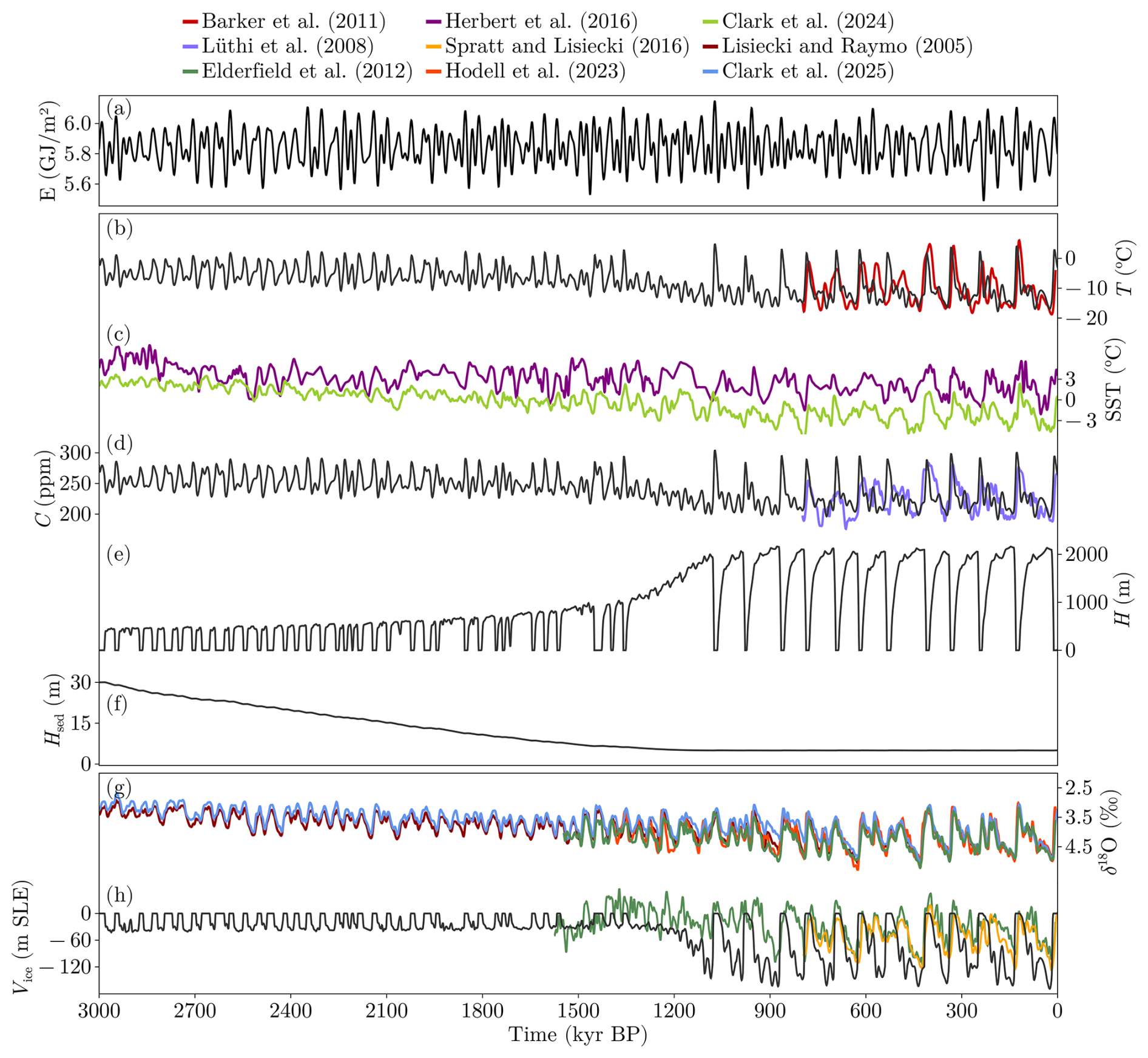
Figure B2 BASE experiment using CSI forcing (BASE-CSI). Note that we employed $f_{\dot{p}}={\mathrm{10}}^{-\mathrm{7}}$ (−29 % of the original value in the CSI experiment) and $f_v=\mathrm{1.15}\times {\mathrm{10}}^{-\mathrm{5}}$ (−62 % of the original value in the CSI experiment). (a) Boreal SSI, (b) regional air temperature anomaly with respect to T_ref in comparison with Barker et al. (2011), (c) global-mean sea-surface temperature (SST) from Herbert et al. (2016) and Clark et al. (2024). (d) CO₂ concentration compared with Lüthi et al. (2008), (e) ice thickness, (f) sediments thickness, (g) δ¹⁸O from Lisiecki and Raymo (2005), Elderfield et al. (2012), Ahn et al. (2017) and Hodell et al. (2023), and (h) ice volume time series in comparison with Elderfield et al. (2012), Spratt and Lisiecki (2016) and Clark et al. (2025). Note that black curves all represent results simulated with PACCO.

Appendix C: Wavelet transforms of some TREND-C experiments

Figure C1 shows the normalized spectral power (NSP) as a function of time for NOSEDIM-low and 4 TREND-C experiments.

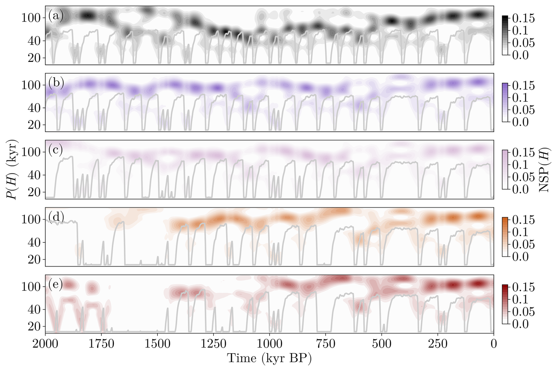
Figure C1 NSP as a function of time for NOSEDIM-low and 4 emblematic cases of the TREND-C experiments. Note that the associated H is plotted in grey as a reference. (a) Interactive carbon cycle and the trend applied in the rows below is (b) −0.05, (c) −0.12, (d) −0.20 and (e) $-\mathrm{0.23}\mathrm{ppm}{\mathrm{kyr}}^{-\mathrm{1}}$.