The oxygen valve on hydrogen escape since the great oxidation event

The Great Oxidation Event (GOE) was a 200 Myr transition circa 2.4 billion years ago that converted the Earth's anoxic atmosphere to one where molecular oxygen (O₂) was abundant (volume mixing ratio $>{\mathrm{10}}^{-\mathrm{4}}$). This significant rise in O₂ is thought to have substantially throttled hydrogen (H) escape and the associated water (H₂O) loss. Atmospheric estimations from the GOE onward place O₂ concentrations ranging between 0.1 % to 150 % PAL, where PAL is the present atmospheric level of 21 % by volume. In this study we use WACCM6, a three-dimensional Earth System Model to simulate Earth's atmosphere and predict the diffusion-limited escape rate of hydrogen due to varying O₂ post-GOE. We find that O₂ indirectly acts as a control valve on the amount of hydrogen atoms reaching the homopause in the simulations: less O₂ leads to decreased O₃ densities that reduce local tropical tropopause temperatures by up to 17 K, which increases H₂O freeze-drying and thus reduces the primary source of hydrogen in the considered scenarios. The maximum differences between all simulations in the total H mixing ratio at the homopause and the associated diffusion-limited escape rates are a factor of 3.2 and 4.7, respectively. The prescribed CH₄ mixing ratio (0.8 ppmv) sets a minimum diffusion escape rate of $\approx \mathrm{2}\times {\mathrm{10}}^{\mathrm{10}}$ mol H yr⁻¹, effectively a negligible rate when compared to pre-GOE estimates (∼10¹²–10¹³ mol H yr⁻¹). Because the changes in our predicted escape rates are comparatively minor, our numerical predictions support geological evidence that the majority of Earth's hydrogen escape occurred prior to the GOE. Our work demonstrates that estimations of how the tropical tropopause layer and the associated hydrogen escape rate evolved through Earth's history requires 3D chemistry-climate models which include a global treatment of water vapour microphysics.

1 Introduction

A key component of Earth's atmospheric and biological history is its water (H₂O). The relative amount of H₂O that was present during the Earth's formation versus the quantity delivered by volatile-rich bodies (e.g., comets and asteroids; Dauphas et al., 2000; Izidoro et al., 2013), as well as the H₂O lost to space through hydrogen escape (Catling et al., 2001; Genda and Ikoma, 2008), or exchanged into the interior (Hallis et al., 2015; Korenaga et al., 2017), has had an important impact on how the Earth's surface and the atmosphere have developed. Beyond Earth, the solar system's terrestrial planet atmospheres are desiccated and consequently, Venus and Mars are both apparently desolate environments. It's possible that Venus was never habitable (Turbet et al., 2021; Warren and Kite, 2023; Constantinou et al., 2024), but Mars was likely habitable early in its history before its water was isolated to the subsurface and the crust (di Achille and Hynek, 2010; Orosei et al., 2018; Scheller et al., 2021; Lauro et al., 2021; Sauterey et al., 2022; Zheng et al., 2024; Wright et al., 2024). Venus is now too hot for liquid H₂O to persist and probably lost much of its natal H₂O through atmospheric hydrogen escape (Ingersoll, 1969; Kulikov et al., 2006; Kane et al., 2019; Gu et al., 2025).

In contrast, Earth has mostly remained temperate throughout its history, with liquid water persisting on the surface for over 4 billion years (Feulner, 2012, and references therein), although there were periods of widespread glaciation at either end of the Proterozoic eon (2.4–0.541 Gyr ago; Young, 2013; Warke et al., 2020). A mostly temperate Earth has been possible despite a fainter Sun in Earth's past (Bahcall et al., 2001; Feulner, 2012; Charnay et al., 2020), in combination with fluctuations in albedo (Charnay et al., 2020; Goldblatt et al., 2021) and atmospheric composition, in particular the greenhouse gases CO₂ (Sheldon, 2006, 2013; Kanzaki and Murakami, 2015) and CH₄ (Daines and Lenton, 2016; Zhao et al., 2018; Laakso and Schrag, 2019; Fakhraee et al., 2019). Geochemical proxies suggest a broad range but generally greater past abundance for CO₂, whereas only loose constraints have been placed on CH₄ (Catling and Zahnle, 2020, and references therein), with debates regarding whether CH₄ during the Proterozoic was higher or lower in abundance than present day still ongoing (see Discussion section).

As all known life requires liquid H₂O, the history of Earth's H₂O is inextricably tied to the evolution of Earth's life. From isotopic evidence and computational modelling, since its formation, the Earth may have lost between 0.13 and 2 times the present ocean volume (Pope et al., 2012; Kurokawa et al., 2018; Zahnle et al., 2019). Indeed, the early Archean Earth (4–2.4 Gyr ago), before 3.2 Gyr ago, may have been fully covered in a global ocean (Dong et al., 2021). The current hydrogen escape rate is $\approx \mathrm{4}\times {\mathrm{10}}^{\mathrm{10}}$ mol of H yr⁻¹, corresponding to roughly 1 m of global water loss per 1 billion years (Zahnle et al., 2013). Given that the Earth's ocean can be up to 11 km deep (Gardner et al., 2014), and its mean depth is ≈3.6 km (Charette and Smith, 2010), the loss rate is insignificant. This suggests a different past for hydrogen escape than the constant modern rate would imply.

Therefore, an important but uncertain component of Earth's water loss is determining the amount of hydrogen (H) that has escaped to space. As the lightest element, H escapes atmospheres more readily than other elements and chemical compounds. On Earth, hydrogen atoms exist in many different chemical species in the lower and middle atmosphere (Brasseur and Solomon, 2005). The four major chemical constituents that contribute hydrogen atoms to the upper atmosphere, and therefore the species we focus on in this work, are H, H₂, H₂O, and CH₄. Atmospheric escape of hydrogen can occur from a planet through several mechanisms, including: Jeans escape, hydrodynamic flow, sputtering, impacts, photochemical escape, and charge exchange escape (Lundin et al., 2007; Johnson, 2010; Shematovich and Marov, 2018; Gronoff et al., 2020). For these mechanisms, with the exception of impacts and hydrodynamic flow, the hydrogen escapes from the exosphere at the top of the atmosphere. In such cases, hydrogen cannot escape faster than it can be delivered to the exosphere through molecular diffusion. This is known as “diffusion-limited hydrogen escape” (Hunten, 1973; Hunten and Donahue, 1976; Walker, 1977; Kasting and Catling, 2003; Zahnle et al., 2013). The diffusion-limited rate of hydrogen escape is set by two controlling bottlenecks, the upward diffusion of hydrogen atoms (mostly in H₂O and CH₄) through the tropopause “cold trap”, and the upward diffusion of hydrogen atoms through molecular diffusion above the homopause¹ (Catling et al., 2001; Catling and Kasting, 2017).

The primary hydrogen bottleneck, the cold trap, is where the saturation mixing ratio of H₂O and ice is at a minimum, such that it modulates the amount of H₂O propagating upwards into the stratosphere (Kasting et al., 2015). On Earth, the cold trap is typically described as the tropical tropopause layer (TTL). The TTL is three-dimensional and is defined as the transition region between the Hadley circulation in the troposphere and the start of the deep branch of the Brewer-Dobson circulation (Brasseur and Solomon, 2005; Fueglistaler et al., 2009; Glanville and Birner, 2017). Despite being located above the tropics (at 12–16 km in altitude, which is 70–150 hPa in pressure), which have on average greater surface temperatures than higher latitudes, the TTL is defined by its cold temperatures (Brasseur and Solomon, 2005; Fueglistaler et al., 2009). The cause of this is adiabatic cooling as air is transported upwards from the convective troposphere into the stratosphere, and this cold temperature region leads to the removal of water vapor from the atmosphere through condensation (Brewer, 1949; Newell and Gould-Stewart, 1981; Danielsen, 1982; Pommereau and Held, 2007). The location, temperatures, and dynamics of the TTL are affected by seasons (Kim and Son, 2012) and climate change (Randel and Jensen, 2013; Lin et al., 2017; Zou et al., 2023; Zolghadrshojaee et al., 2024). Of the major H-bearing species, only H₂O is significantly affected by temperatures in the TTL, whereas H₂ and CH₄, which don't condense in Earth's atmosphere, are unaffected by the cold trap mechanism.

In the stratosphere, hydrogen atoms are interchanged between CH₄, H₂O and H₂, until reaching the homopause (Catling and Kasting, 2017). At altitudes exceeding the homopause, through diffusive separation, the lighter atmospheric constituents with lower molecular masses increase in relative abundance with decreasing pressure (e.g., H, He, O, and N). Note that H₂ would also increase but it is rapidly photodissociated into H. Hence, above the homopause, H dominates the total hydrogen budget (Catling and Kasting, 2017).

The atmosphere of the Archean Earth was likely weakly reducing with greater quantities of CH₄, CO, and H₂ (Kasting et al., 2001; Kharecha et al., 2005; Kadoya and Catling, 2019; Catling and Zahnle, 2020). Midway through Earth's history, approximately 2.4 billion years ago, a rise in oxygen known as the Great Oxidation Event (GOE; Farquhar et al., 2000; Holland, 2002; Hodgskiss et al., 2019; Warke et al., 2020; Goldblatt et al., 2021) has been proposed to have significantly reduced hydrogen escape from ∼10¹²–10¹³ to ∼10¹⁰ mol H yr⁻¹ (Catling et al., 2001; Zahnle et al., 2013). This is because an oxygenated atmosphere destroys reducing species (e.g., H₂ and CH₄), resulting in lower amounts of such gases which contribute hydrogen atoms to the upper atmosphere.

In conjunction, atmospheric escape of hydrogen may have played a significant role in shaping Earth's atmosphere through time. It is thought to at least be partially responsible for oxidising the Earth's surface: when H₂O is photodissociated above the troposphere, the liberated hydrogen (H) can escape to space, and the oxygen (O) left behind oxidises the Earth (Catling et al., 2001; Claire et al., 2006; Zahnle et al., 2013). Alongside photosynthetic production of O₂ from cyanobacteria, this process is hypothesized to have contributed to the occurrence of the GOE because the process of hydrogen escape and subsequent oxidation is irreversible, leading to a reduced sink of O₂ over time (Catling et al., 2001; Claire et al., 2006; Zahnle et al., 2013). Nevertheless, considerable uncertainty persists regarding the precise temporal evolution of Earth's atmosphere (Kasting, 2025), with hydrogen escape a key aspect of the holistic picture.

There is no direct way to determine the amount of hydrogen that has escaped in Earth's history. As mentioned, several measurements can be used to infer this quantity, and the chronology of one of the heaviest gases, Xe, may be informative. Xe is more easily ionised compared to the other noble gases which do not exhibit the same fractionation (the so-called Xenon paradox; Anders and Owen, 1977; Zhu et al., 2013). It was proposed that Xe⁺ could escape Earth's atmosphere when propelled by H⁺ ions, and this has been shown to be a feasible physical process (Zahnle et al., 2019). Accordingly, the timing of Earth's Xe fractionation (see Fig. 3 in Zahnle et al., 2019) may trace high levels of atmospheric hydrogen escape during the Archean eon. There has been relatively small changes in Xe fractionation since the GOE (Avice et al., 2018), indicating the vast majority of historical hydrogen escape occurred prior to this time (i.e., before ∼2.4 Gyr ago).

Whilst hydrogen escape rates may have been much lower in the last ∼2.4 Gyr, to our knowledge, no work has quantitatively estimated escape rates since the GOE occurred using a 3D model. In this work, we build upon a previous study (Cooke et al., 2022) which simulated a range of O₂ concentrations that may have been present on the Earth for the last 2.4 Gyr and found that lower O₃ columns were predicted compared to previous work (Kasting and Catling, 2003; Segura et al., 2003; Rugheimer et al., 2015; Rugheimer and Kaltenegger, 2018; Kaltenegger et al., 2020; Ji et al., 2023). More recent work has in part supported the results of lower O₃ for a given O₂ mixing ratio (Yassin Jaziri et al., 2022; Ji et al., 2024; Liu et al., 2025). O₃ and its associated UV heating is responsible for the temperature inversion that creates the Earth's stratosphere, and this heating affects the temperatures in the TTL. Therefore, the O₂ fluctuations following the GOE may have modulated the upward transport of H₂O through the TTL and consequently, hydrogen escape too.

Using the 3D chemistry-climate model WACCM6, we first explore the effect of changing the O₂ abundance on the TTL region, before investigating the influence it may have had on hydrogen escape during the Proterozoic eon. Our aim is to estimate how changes to atmospheric O₂ alone can affect the diffusion-limited hydrogen escape rate. In terms of hydrogen escape fluctuations, our focus is on H₂O, and we hold the mixing ratios of H₂ and CH₄ constant at the surface. We note that CO₂, CH₄ and H₂ are likely to have varied during the past 2.4 billion years (Catling and Zahnle, 2020), as will have the luminosity of the Sun (Feulner, 2012). These variables are important because CH₄ and H₂ are key hydrogen carriers to the upper atmosphere, and additionally CH₄ and CO₂ provide greenhouse warming which can affect TTL temperatures. The TTL will also have been affected by the reduced total insolation from a younger Sun which would act to cool the troposphere. The purpose of this work is, however, to present the mechanism by which O₂ affects hydrogen escape. We calculate such H escape deviations, paving the way for future work on the topic to investigate other physical, chemical, and biological influences.

2 Numerical methods

2.1 WACCM6 model

The simulations we analyse are those from Cooke et al. (2022), where the Earth System Model WACCM6 (Gettelman et al., 2019) was employed to model different oxygenation levels. WACCM6 is a configuration of the Coupled Earth System Model (CESM), and we use version 2.1.3 (CESM2.1.3, https://www.cesm.ucar.edu/models/cesm2,last access: 2 March 2026) with minor code alterations in the initial conditions (ExoCESM GitHub: https://github.com/exo-cesm/CESM2.1.3/tree/main/O2_Earth_analogues, last access: 2 March 2026), which we describe in this section.

The first simulation we perform commences with initial conditions which are intended to be representative of Earth's pre-industrial (PI) atmosphere circa 1850, alongside contemporary ocean and land settings, and the current orbital setup with a 23.4° obliquity and 24 h rotation rate. Deep time paleoclimate studies often change the continents and we accept that this is a limitation with the WACCM6 model where continents cannot currently be modified. The circulation pattern and climate would have been different in the past due to various factors, which include the younger Sun, different greenhouse gas concentration, and the formation and break up of supercontinents such as Pangea and Columbia/Nuna (Rogers and Santosh, 2002; Feulner, 2012; Fiorella and Sheldon, 2017; Catling and Zahnle, 2020). The model's spatial resolution for the atmosphere was set at 1.875° latitude by 2.5° longitude (yielding a 96×144 horizontal grid). This configuration utilizes 70 atmospheric layers in vertical pressure coordinates extending from the surface (approximately 1000 hPa) to the thermosphere ($\mathrm{4.5}\times {\mathrm{10}}^{-\mathrm{6}}$ hPa, or ∼150 km). The land component (CLM5.0) operates on the same 1.9°×2.5° horizontal grid as the atmosphere to maintain consistency in surface flux exchanges. The simulation employs an interactive ocean via the POP2 model, which operates on a 1° displaced-pole grid. This ocean grid features 320×384 points, with enhanced latitudinal resolution near the equator to better resolve tropical dynamics. This same grid is utilized by the Sea-Ice (CICE5) and Wave (WaveWatch3) components. Additionally, freshwater discharge is included in the MOSART river transport model on a 0.5° global grid.

Both atmospheric and oceanic components of the model are interactive, allowing dynamic responses to environmental stimuli like temperature changes. Our simulations incorporated middle atmosphere chemistry as described by Emmons et al. (2020), featuring 98 chemical species and 298 reactions, including O₃ chemistry. The atmospheric time step, Δt, was set at 30 min. The concentrations of 75 species were computed using an implicit numerical scheme, while 22 long-lived species were computed using an explicit numerical scheme (Sandu et al., 1997; Brasseur and Solomon, 2005). N₂ is considered invariant. Absorption of light by CO₂ and H₂O in the Schumann-Runge (S-R bands) is not included in these simulations, and neither is scattering at wavelengths <200 nm. For more details on the inclusion of these processes, we refer the reader to Ji et al. (2023) and Ji et al. (2024), as well as Sect. 4.2 where we discuss how it might impact our results.

In total, eight simulations were performed for the Earth system with different mixing ratios of atmospheric O₂, where the atmospheric pressure was kept the same by changing the abundance of the background gas, N₂. O₂ mixing ratios are given in terms of present atmospheric level (PAL), which is 21 % by volume. The O₂ surface mixing ratios span values between 0.1 %–150 % PAL, which are within estimates for the Earth over the last 2.4 billion years (Lyons et al., 2014; Large et al., 2019; Catling and Zahnle, 2020; Steadman et al., 2020). These temporal estimates do not always agree, so we remain agnostic and perform simulations covering the whole range. The simulation names are PI, 150 % PAL, 50 % PAL, 10 % PAL, 5 % PAL, 1 % PAL, 0.5 % PAL, and 0.1 % PAL. CO₂, CH₄, N₂O, and H₂, were held fixed at values of 284 ppmv, 0.8 ppmv, 273 ppbv, and 0.5 ppmv, respectively. The mixing ratios or fluxes of gases specified at the surface were kept constant as O₂ was altered. This assumption is likely not realistic for the entirety of the last 2.4 Gyr, but it allows us to isolate the role O₂ changes make to the chemistry and dynamics of the atmosphere. Water vapor feedback, in terms of evaporation and rainout, is included in WACCM6, but hydrogen escape and water loss are not explicitly simulated. Instead, we estimate these values once quasi-steady state has been reached in the simulation (see Sect. 2.2).

We average the outputs of the WACCM6 simulations over the last four years of the simulation once the middle atmospheric (defined here as between 12–100 km in altitude; Brasseur and Solomon, 2005) trend in total hydrogen atoms has halted, and this required between 30 and 90 simulations years for the different scenarios.

2.2 Diffusion-limited hydrogen escape rate

The diffusion-limited hydrogen escape rate (Hunten, 1973; Kasting and Catling, 2003), Φ_esc, is proportional to the total mixing ratio of hydrogen-bearing species, f_T(H), at the homopause:

$$\begin{array}{}\text{(1)}& {\mathrm{\Phi }}_{\mathrm{esc}}\propto f_{\mathrm{T}}\left(\mathrm{H}\right),\end{array}$$

where f_T(H), can be written as

$$\begin{array}{}\text{(2)}& f_{\mathrm{T}}\left(\mathrm{H}\right)=f\left(\mathrm{H}\right)+\mathrm{2}f\left({\mathrm{H}}_{\mathrm{2}}\right)+\mathrm{2}f\left({\mathrm{H}}_{\mathrm{2}}\mathrm{O}\right)+\mathrm{4}f\left({\mathrm{CH}}_{\mathrm{4}}\right)\mathrm{\dots },\end{array}$$

and so on, accounting for all hydrogen-bearing species. We focus on evaluating the abundances of H, H₂, H₂O, and CH₄. In modern Earth's atmosphere, at the tropopause, the H₂ and CH₄ mixing ratios are ≈0.55 ppmv (Catling and Kasting, 2017) and ≈1.9 ppmv (Saunois et al., 2025), respectively. There, the H₂O mixing ratio varies between ≈2.5–4.5 ppmv, with a mean stratospheric entry value of ∼3.5–4 ppmv (Fueglistaler et al., 2009; Gettelman et al., 2019). This puts the stratospheric entry value of total hydrogen at ∼17 ppmv, although with CH₄ at a lower concentration during the pre-industrial period, the entry value would be closer to ∼12 ppmv. In our simulations, the lower boundary mixing ratios are instead mixing ratios of 0.5 and 0.8 ppmv for H₂ and CH₄, respectively, corresponding to pre-industrial values. Consequently, H₂O is the primary carrier of hydrogen atoms to the middle atmosphere. Other H-bearing species such as OH, HO₂, and H₂O₂ are included in the WACCM6 model but are not sufficiently abundant to contribute significantly to the overall hydrogen budget.

The calculation of Φ_esc at the homopause can be made by considering the binary diffusion coefficients which depend on the temperature of the atmosphere and the chemical species. Φ_esc, in units of atoms cm⁻² s⁻¹, is given by

$$\begin{array}{}\text{(3)}& {\mathrm{\Phi }}_{\mathrm{esc}}=\sum _{i=\mathrm{1}}^n{\displaystyle \frac{N_{i}f\left(i\right)b_i}{H_{\mathrm{h}}}},\end{array}$$

where H_h is the atmospheric scale height at the homopause, N_i is the number of hydrogen atoms in each chemical species, i, and b_i is the binary diffusion parameter for each constituent. The binary diffusion coefficient depends on the temperature of the atmosphere at the homopause (T_h), the masses of the species, and their collision cross-sections. For each species considered here, the binary diffusion coefficients are $b_{\mathrm{H}}=\mathrm{6.5}\times {\mathrm{10}}^{\mathrm{17}}{T}_{\mathrm{h}}^{\mathrm{0.7}}$, $b_{{\mathrm{H}}_{\mathrm{2}}}=\mathrm{2.67}\times {\mathrm{10}}^{\mathrm{17}}{T}_{\mathrm{h}}^{\mathrm{0.75}}$, $b_{{\mathrm{H}}_{\mathrm{2}}\mathrm{O}}=\mathrm{0.137}\times {\mathrm{10}}^{\mathrm{17}}{T}_{\mathrm{h}}^{\mathrm{1.072}}$, $b_{{\mathrm{CH}}_{\mathrm{4}}}=\mathrm{0.734}\times {\mathrm{10}}^{\mathrm{17}}{T}_{\mathrm{h}}^{\mathrm{0.750}}$. These binary diffusion parameters for H, H₂, and H₂O are sourced from Hunten (1973) and CH₄ is sourced from Banks and Kockarts (1973). The calculations are made for the whole atmosphere (latitude and longitude at the homopause) before calculating a longitudinally-averaged and latitudinally-weighted mean.

From Earth's exosphere, hydrogen escapes faster than it is delivered, such that throughout this work, we will assume that the loss rate of hydrogen atoms is diffusion-limited (ignoring hydrodynamic escape and impacts). Note that it is possible for hydrogen to escape slower than this upper limit, provided the rate of loss from the exosphere is the limiting factor (e.g., energy-limited escape, photon-limited escape; Tian et al., 2005; Salz et al., 2016; Owen and Alvarez, 2016; Lehmer and Catling, 2017).

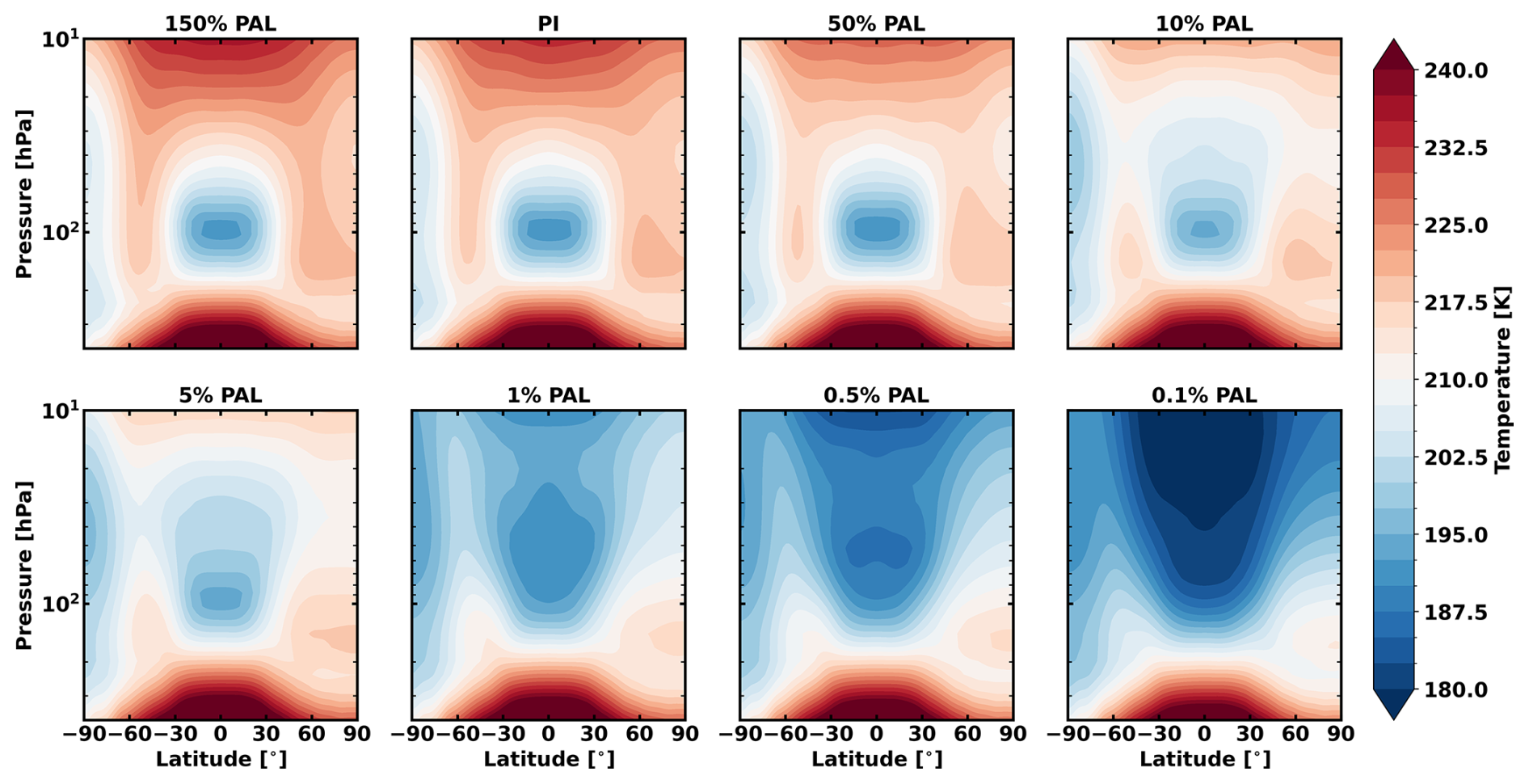
Figure 1 The zonal mean of atmospheric temperature (in K) is shown for simulations with O₂ mixing ratios between 150 % PAL and 0.1 % PAL, where O₂ decreases in abundance from the top left panel to the bottom right panel. The colour bar shows hotter temperatures in red and colder temperatures in blue. The TTL region is ±23.4° from the equator and between 70–150 hPa in pressure.

3 Results

As part of the hydrological cycle, liquid water evaporates from the surface and warm, moist air rises due to buoyancy. Hence, rivers, lakes, and predominantly the ocean, act as a sources of hydrogen atoms to the atmosphere. We will present the results in terms of how the total hydrogen mixing ratio starts at the surface and how it changes with decreasing atmospheric pressure (increasing altitude). This includes tracking the proportion of hydrogen atoms bound in different species, such as H₂O and CH₄. We will show how the O₂ mixing ratio affects the total hydrogen mixing ratio through the atmosphere and ultimately the amount of hydrogen atoms diffusing up to the exosphere. In the following subsection, we consider how O₂ affects clouds, condensation, and the cold trap at the top of the troposphere. These processes act to keep hydrogen atoms in the troposphere that would otherwise mix into the stratosphere and upwards to eventually escape to space.

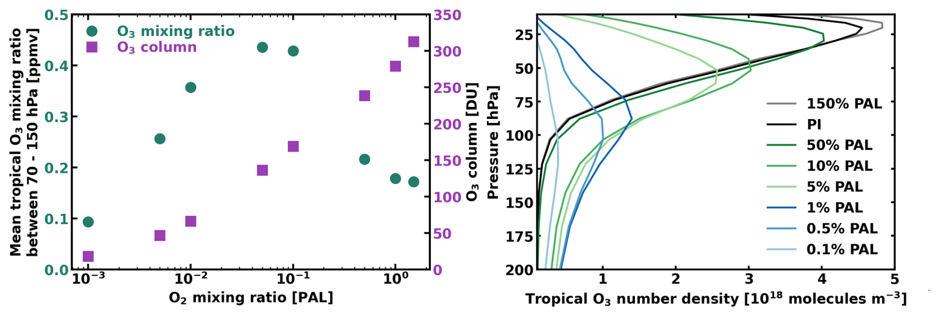
Figure 2 Left: The mean tropical (defined at latitudes ±24° from the equator) O₃ mixing ratio between 70–150 hPa is plotted on the left vertical axis in teal circles against the atmospheric mixing ratio of O₂ at the surface in terms in terms of the present atmospheric level (PAL), which is 21 % by volume. The total global ozone (O₃) column density in Dobson Units (DU, where 1 DU $=\mathrm{2.69}\times {\mathrm{10}}^{\mathrm{20}}$ molec. m⁻²) is also plotted in purple squares on the right vertical axis against the atmospheric mixing ratio of O₂. Right: The O₃ number density is shown for all eight simulations between 10–200 hPa on a linear scale (note the number density does not go to zero at pressures greater than 200 hPa, see Cooke et al., 2022).

3.1 Water vapour through the cold trap

In every simulation, the global mean mixing ratio of each species at the surface for H₂O, H, CH₄, and H₂, is ∼10 000, $<{\mathrm{10}}^{-\mathrm{8}}$, ≈0.8, and ≈0.5 ppmv respectively, with the latter two molecules specified with fixed mixing ratios at the surface. As temperature and pressure decline with altitude in the troposphere, the atmosphere cannot hold as much H₂O vapor. This is because the drop in pressure causes the air to cool (adiabatic cooling), and the saturation vapor pressure of water, which determines the air's capacity for water vapor, is strongly dependent on temperature. Figure 1 presents the zonal mean (averaged over longitude) of the atmospheric temperature between the surface and 10 hPa (∼30 km in altitude) for all the WACCM6 simulations. The temperature structure of the atmosphere is set by the strength and spectral shape of the incoming radiation, the moist adiabat in the troposphere, atmospheric composition (providing heating and cooling in different layers), clouds and ice, and atmospheric dynamics. Between 150 % PAL and 50 % PAL, the temperature structure at pressures greater than 10 hPa (or altitudes below 10 hPa) is similar. At 10 % and 5 % PAL, the temperature increases in the middle atmosphere, and this is noticeable in the tropics between 200–30 hPa. At ≤1 % PAL of O₂, the stratosphere begins to become significantly cooler, with the 10 hPa pressure level ∼60 K cooler in the 0.1 % PAL simulation compared to the 150 % PAL simulation. A globally averaged stratospheric temperature inversion of ≈2 and ≈1 K exists in the 1 % PAL and 0.1 % PAL simulations, respectively, which is significantly smaller than the ≈60 K temperature inversion in the PI atmosphere.

Figure 2 shows the mixing ratio of atmospheric O₂ plotted against the O₃ column density, as well as the mean O₃ mixing ratio between 70 and 150 hPa in the tropical region, accounting for the expanse of the TTL. The figure also shows the O₃ number density in the tropics between 10 and 200 hPa. Whilst the global O₃ column density increases with increasing O₂ mixing ratio, this is not the case for the O₃ mixing ratio around the TTL region: there is instead a peak at ≈5–10 % PAL. The O₃ number density also mirrors this relationship. When O₂ is decreased, O₃ accumulates lower down in the atmosphere because the wavelengths that photolyse O₂ to produce “odd oxygen” (O + O₃) are able to penetrate deeper. Consequently, for O₂ concentrations of ≤10 % PAL, O₃ maximizes in this region near the TTL. The TTL temperatures are a balance between shortwave heating and the emission and absorption of longwave radiation. Whilst this causes higher temperatures than the PI atmosphere for 5 %–10 % PAL, simulations with ≤1 % PAL have resultant lower temperatures. This effect is a local TTL phenomenon; globally, the mean tropopause temperatures decrease with decreasing O₂.

These results are in line with previous O₃ depletion experiments (albeit of a much smaller magnitude) which found that reduced O₃ concentrations cooled the TTL and led to less stratospheric water vapour (Forster et al., 2007; Xie et al., 2008; Lu et al., 2021; Zhou et al., 2022). The cooling was attributed to radiative processes. Indeed, Forster et al. (2007) showed that less O₃ in the tropical lower stratosphere caused cooling that extended into the upper tropical troposphere due to reduced downward longwave radiation. Similarly, here we find that lower middle stratospheric densities of O₃ reduces the propagation of longwave radiation downwards. This mechanism is the cause of the hotter temperatures in the higher oxygenated scenarios in Fig. 1 compared to scenarios with ≤1 % PAL. This is also why there is an asymmetry in temperatures because of hemispherical asymmetries in the O₃ distribution (there is more O₃ in the northern hemisphere) as a result of the Brewer-Dobson circulation (Dobson and Harrison, 1926; Brewer, 1949; Butchart, 2014).

In Sect. 1, we described how H₂O moves through the TTL to get into the stratosphere on modern Earth. The cold trap mechanism is indirectly sensitive to O₂ concentrations resulting from the aforementioned difference in O₃ and hence UV heating. Due to the difference in time-averaged zonal mean TTL temperatures between the PI and 0.1 % PAL simulations of up to ≈17 K, more H₂O is frozen out in the form of water clouds, ice, and ice clouds (e.g., cirrus clouds; Wang and Dessler, 2012) before crossing ≈100 hPa in the 0.1 % PAL case compared to the standard PI case. Stratospheric O₃ and H₂O are greenhouse gases, and with less H₂O reaching the stratosphere as a consequence of reduced O₃, this decreases tropospheric heating (Deitrick and Goldblatt, 2023), causing a positive feedback effect, albeit a small one: there is some cooling at the surface, but this is limited to <3 K in terms of global averaged surface temperatures.

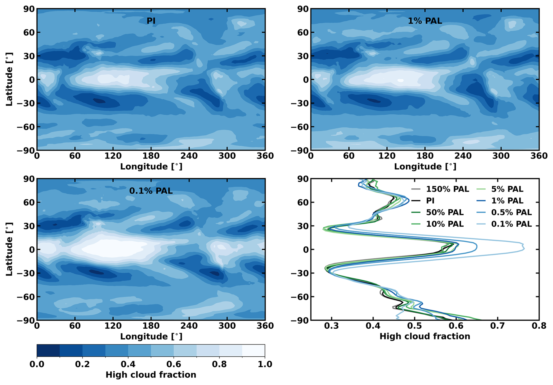
Figure 3 The top left, top right, and bottom left panels show the high cloud fraction as a function of longitude and latitude for the PI, 1 % PAL, and 0.1 % PAL scenarios, respectively. Bottom right: The high cloud fraction (high clouds are defined as clouds at pressures <400 hPa) is averaged over longitude and shown as a function of latitude for all the WACCM6 simulations.

The fractional coverage of high clouds (high clouds are defined as clouds at pressures <400 hPa and are therefore relevant to the TTL) versus latitude is shown in Fig. 3. The coverage of high clouds for the PI, 1 % PAL, and 0.1 % PAL is also shown in the same figure. The O₂ mixing ratio affects high cloud coverage across the entire planet, but especially in the tropics. There is a ≈30 % increase in the peak high cloud fraction at the equator (0° latitude) from the 150 % PAL simulation to the 0.1 % PAL simulation, although the peak high cloud fraction for the simulations between the O₂ concentrations of 150 % PAL to 1 % PAL at the equator all fall within 6 % of each other. Low clouds (surface – 700 hPa) and medium clouds (700–400 hPa) exhibit very little deviation between the simulations.

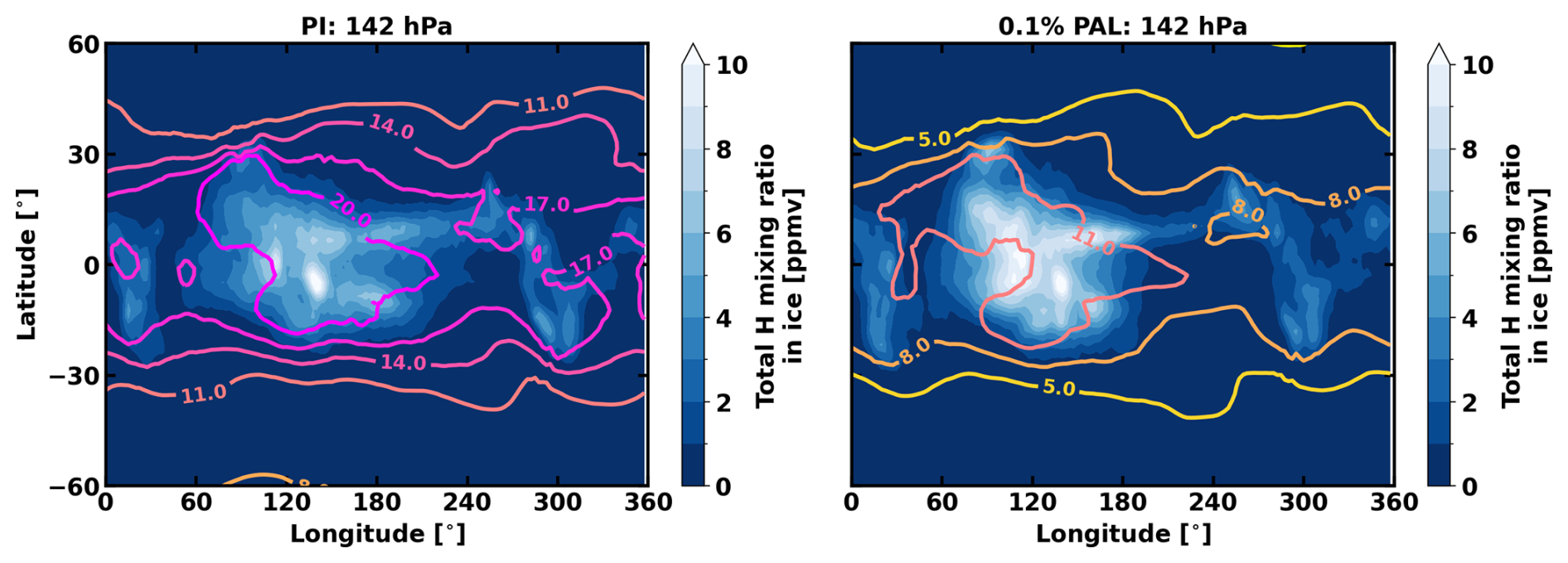
Figure 4 The atmospheric ice content (blue-white shading) and the amount of atmospheric H₂O (magenta-orange-yellow contours) is shown on the latitude-longitude grid of the Earth. Both are given in terms of ppmv. The PI simulation (left) and the 0.1 % PAL simulation are shown (right). Both scenarios are shown for a pressure level of 142 hPa, which corresponds to an altitude of ≈14 km near the base of the TTL.

The total hydrogen mixing ratio bound in ice (ice water content and ice clouds) and H₂O for the PI and 0.1 % PAL cases is shown in Fig. 4 between −60 to +60° latitude. At 142 hPa (roughly 14 km in altitude), the 0.1 % PAL scenario has a greater amount of ice content and a lower amount of H₂O. Thus, due to the freeze-drying of the atmosphere, fewer hydrogen atoms are able to contribute to the stratospheric total hydrogen mixing ratio, f_T(H), when compared to the PI case. Both simulations show a larger build-up of total ice water, ice clouds, and H₂O content over the western pacific (e.g., between 90–150° E), as is found on modern Earth (Newell and Gould-Stewart, 1981; Dessler, 1998; Dong et al., 2020).

In the cases we have simulated, the interplay between UV radiation, O₂ mixing ratio, and 3D transport, is especially important for predicting the O₃ distribution. The amount of O₃ and the incoming UV affect temperatures around the tropopause, and ultimately how much H₂O can reach the stratosphere. Here we are exploring the impact of O₂ levels alone on the TTL temperatures and thus atmospheric escape. Other factors will have influenced TTL temperatures for the past 2.4 billion years, and these will be discussed in Sect. 4.

3.2 Tropical tape recorder

The tropical “tape recorder” (Mote et al., 1995; Liu et al., 2007; Glanville and Birner, 2017) for H₂O is the phenomenon where seasonal temperature fluctuations in the TTL modulate the mixing ratio of H₂O that enters the stratosphere over an annual cycle. The temperature of the TTL itself is affected by several processes, including radiative heating and cooling, deep convection, sea surface temperatures, and the Quasi-Biennial Oscillation (Fueglistaler et al., 2009; Paulik and Birner, 2012; Garfinkel et al., 2013; Tegtmeier et al., 2020). Note that the tape recorder effect exists for some other molecules too, including CO (Schoeberl et al., 2006; Liu et al., 2007; Pumphrey et al., 2008). The Brewer-Dobson circulation (Dobson and Harrison, 1926; Brewer, 1949; Butchart, 2014), over a period of months, transports H₂O upward (Glanville and Birner, 2017), causing the distinct tape recorder effect (WACCM6 is able to generate this effect – see the PI simulation in Fig. 5 and also Gettelman et al., 2019). The seasonally-varying temperatures in the TTL imprint a record on the observed mixing ratio of H₂O which is altered in the middle atmosphere in the subsequent months.

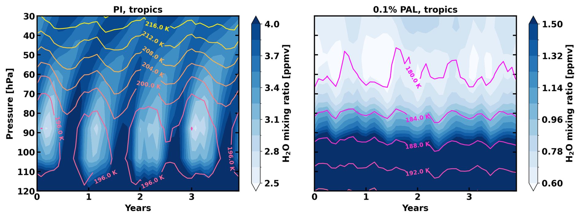
Figure 5 The water vapour mixing ratio in ppmv is shown for the PI scenario (left) and the 0.1 % PAL scenario (right) between pressures of 120–30 hPa. Each panel shows four years in a row of each simulation, displaying the zonally averaged and latitudinally weighted H₂O mixing ratio in the tropics between ±24°. Whites show the lowest mixing ratios and darker blues show progressively larger mixing ratios. Note the different scales on each colour bar. The contours show the atmospheric temperature in kelvin, with yellow indicating higher temperatures and magenta indicating lower temperatures.

In the PI simulation, the tape recorder is easily visible over a 4-year time frame with a period of 1 year (see Fig. 5). For the PI case, the peak seasonal differences in the tape recorder effect are of order 1.5 ppmv at ≈90 hPa. Note that this amplitude is much smaller than the tape recorder variation Liu et al. (2023) found for an Earth-like exoplanet with a higher eccentricity of 0.4.

At low oxygenation states (<1 % PAL), seasonal differences in temperature and the Brewer-Dobson circulation are still present, but their magnitude is smaller so the tropical tape recorder effect is muted. Whilst the H₂O mixing ratios still vary, the tape recorder effect is no longer visible from the scale shown in Fig. 5 at 0.1 % PAL because there is no clear periodic signal. Variance-preserving Fourier spectra show that the annual harmonic (1 cycle per year) dominates the stratospheric H₂O variability in the PI simulation between 100 and 30 hPa. In contrast, the 0.1 % PAL simulation exhibits a much weaker annual contribution relative to total variance at these pressure levels, consistent with the absence of a tape-recorder signal. Therefore, the seasonal mechanism which transports more water vapour into the stratosphere during warmer periods in the TTL is no longer effective in the 0.1 % PAL case.

3.3 Total hydrogen mixing ratio

After H₂O passes through the cold trap, the first bottleneck for the total hydrogen mixing ratio of temperate Earth-like atmospheres has been passed. We now assess the quantitative effect of this bottleneck, and the relative contributions of each of the four major hydrogen bearing species in our simulations.

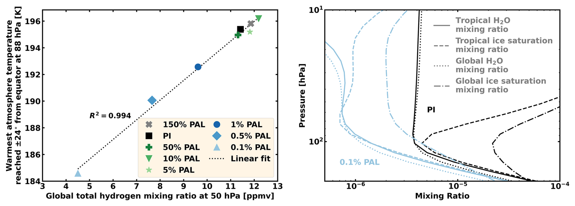
Figure 6 Left: The globally averaged total hydrogen mixing ratio (f_T(H)) at 50 hPa is plotted against the warmest temperature reached within ±24° (tropical latitudes) from the equator at 88 hPa for each simulation. Linear regression gives a coefficient of determination (R²) of 0.994, which is showed by the dotted black line. The different O₂ mixing ratios are shown by various markers: 150 % PAL (grey cross), PI (black square), 50 % PAL (dark green plus), 10 % PAL (green downward triangle), 5 % PAL (light green star), 1 % PAL (dark blue circle), 0.5 % PAL (blue diamond), and 0.1 % PAL (light blue upward triangle). Right: The H₂O mixing ratio is plotted against pressure for the PI (black) and 0.1 % PAL (light blue) simulations, in terms of its tropical (unbroken line) and global (dotted line) average. Also shown is the ice saturation mixing ratio which depends on temperature and pressure and is shown for the tropical (dashed) and global (dash-dotted) average. The tropical average is for latitudes ±24° from the equator.

Figure 6 displays the warmest atmospheric temperature reached in each simulation at a pressure of 88 hPa (≈18 km for Earth's atmosphere)² in the tropics (within ±24° from the equator) against the globally averaged f_T(H) at 50 hPa. There is a strong positive correlation with a coefficient of determination of R²=0.994 between these two variables. This freeze-drying relationship arises because the warmest temperatures in the tropical atmosphere effectively control the maximum amount of water vapor that can be transported upward through to the stratosphere. As a result, there is a weaker correlation present when comparing f_T(H) with the global mean temperature at the same pressure level, and worse correlation still when comparing to the warmest temperature found anywhere at 88 hPa.

More importantly, Fig. 6 also demonstrates how it is the ice saturation vapor pressure (Murphy and Koop, 2005) in the tropical atmosphere that acts to limit the transport of H₂O upwards. The tropical ice saturation mixing ratio curve is within a factor of 1.18 and 1.01 when compared to the globally averaged H₂O mixing ratio at 100 hPa (≈16 km in altitude) for the PI and 0.1 % PAL atmospheres, respectively. When comparing the global ice saturation mixing ratio curve, the discrepancy is a factor of 5.8 and 3.9 times, respectively. This means that 1D models that are based on globally averaged temperatures may overestimate the stratospheric H₂O abundance for Earth-like oxygenated simulations by up to a factor of 6 (accounting for all simulations here, the discrepancy range is 3.8–6.0).

Figure 6 suggests that the warmest TTL temperatures are the controlling factor in each atmospheric scenario, instead of the atmospheric composition. Yet because composition (i.e., the O₂ mixing ratio) is the variable that is altered in each scenario, the atmospheric composition is the controlling factor for the TTL temperatures. Hence, the oxygenation state of the atmosphere is indirectly controlling the upward flow of hydrogen atoms and affecting the diffusion-limited hydrogen escape rate, and this is what we refer to as the “oxygen valve”.

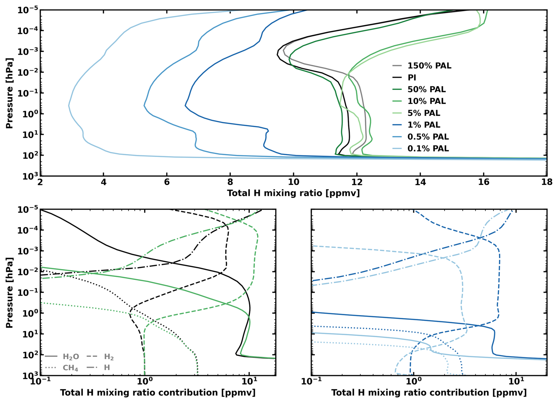
Figure 7 Top: f_T(H), the total hydrogen mixing ratio is given in parts per million by volume (ppmv) and is shown against pressure for the 150 % PAL (grey), PI (black), 50 % PAL (dark green), 10 % PAL (green), 5 % PAL (light green), 1 % PAL (dark blue), 0.5 % PAL (blue), and 0.1 % PAL (light blue) simulations. f_T(H) is calculated using Eq. (2). Hence, the mixing ratio contribution from H, H₂O, H₂, and CH₄ is multiplied by a factor of 1, 2, 2, and 4, respectively. Bottom left: The total hydrogen mixing ratio contribution from H (dash dotted), H₂ (dashed), H₂O (unbroken), and CH₄ (dotted) is shown for the PI and 10 % PAL simulations and bottom right: the 1 % PAL and 0.1 % PAL simulations.

Figure 7 presents the globally averaged f_T(H) vertical profile throughout the atmosphere, which is calculated from Eq. (2) for all the simulations. The mixing ratio of total hydrogen in the stratosphere (at 1 hPa) is f_T(H)=11.7 ppmv in the PI simulation. Turbulent mixing causes f_T(H) to remain roughly constant between the lower stratosphere and homopause. For the 10 % PAL, 1 % PAL, and 0.1 % PAL simulations, the stratospheric f_T(H) values at 1 hPa are approximately 12.4, 6.9, 3.0 ppmv, respectively.

Figure 7 also shows the total hydrogen contribution from the four species that carry the majority of hydrogen atoms (H, H₂, H₂O, and CH₄). These panels show that for the PI simulation (black lines), H₂O is the primary carrier of hydrogen atoms in the lower atmosphere. Above the cold trap in the TTL, the H₂O mixing ratio increases until it reaches a maximum mesospheric value (≈5 ppmv) due to CH₄ reacting with OH. At a pressure of approximately 0.01 hPa, H₂ then becomes dominant. Photolysis of H₂O, CH₄, and H₂, as well as diffusive separation, cause atomic H to become the primary carrier at pressures less than 10⁻⁴ hPa.

Decreasing levels of O₂ act to shift the pressures at which particular species are the principal hydrogen carrier. H₂ begins to increase in abundance at lower altitudes as the atmospheric O₂ concentration is decreased. For instance, with 1000 times less O₂ (0.1 % PAL case, light blue lines), H₂ is dominant at pressures less than 10 hPa, due to both H₂O condensation and photolysis at the higher pressure levels. Again, resulting from diffusive separation, H always dominates towards the top of the model in the lower thermosphere. CH₄ is increasingly lost in the troposphere due to enhanced H₂O photolysis and OH production, acting to reduce CH₄ lifetimes (see the following papers for a more in depth discussion on CH₄ lifetimes: Cooke et al., 2022; Ji et al., 2023, 2024). This loss adds to tropospheric H₂O which is ultimately halted by the cold trap. If the CH₄ mixing ratio at the TTL is greater than half that of H₂O, then CH₄ is the primary contributor to hydrogen escape. However, CH₄ is never the main H carrier in the scenarios we present. As we will discuss later, it is unclear whether this would have been the case for some portions of the Proterozoic.

3.4 Diffusion-limited escape

Now we have assessed f_T(H) throughout the atmosphere we can predict how the rate of diffusion-limited hydrogen escape varies between the different simulated atmospheres with WACCM6. We present the predicted escape rates for each simulation in Table 1.

Table 1 This table shows the eight simulations where the mixing ratio of O₂, given in terms of present atmospheric level (PAL), was varied. The total hydrogen mixing ratio, f_T(H), in ppmv at the homopause, which is taken to be at a pressure of 10⁻³ hPa. The diffusion-limited hydrogen escape rate is given by Φ_esc in mol yr⁻¹ and compared to the predicted escape rate in the PI simulation (Φ_esc,PI).

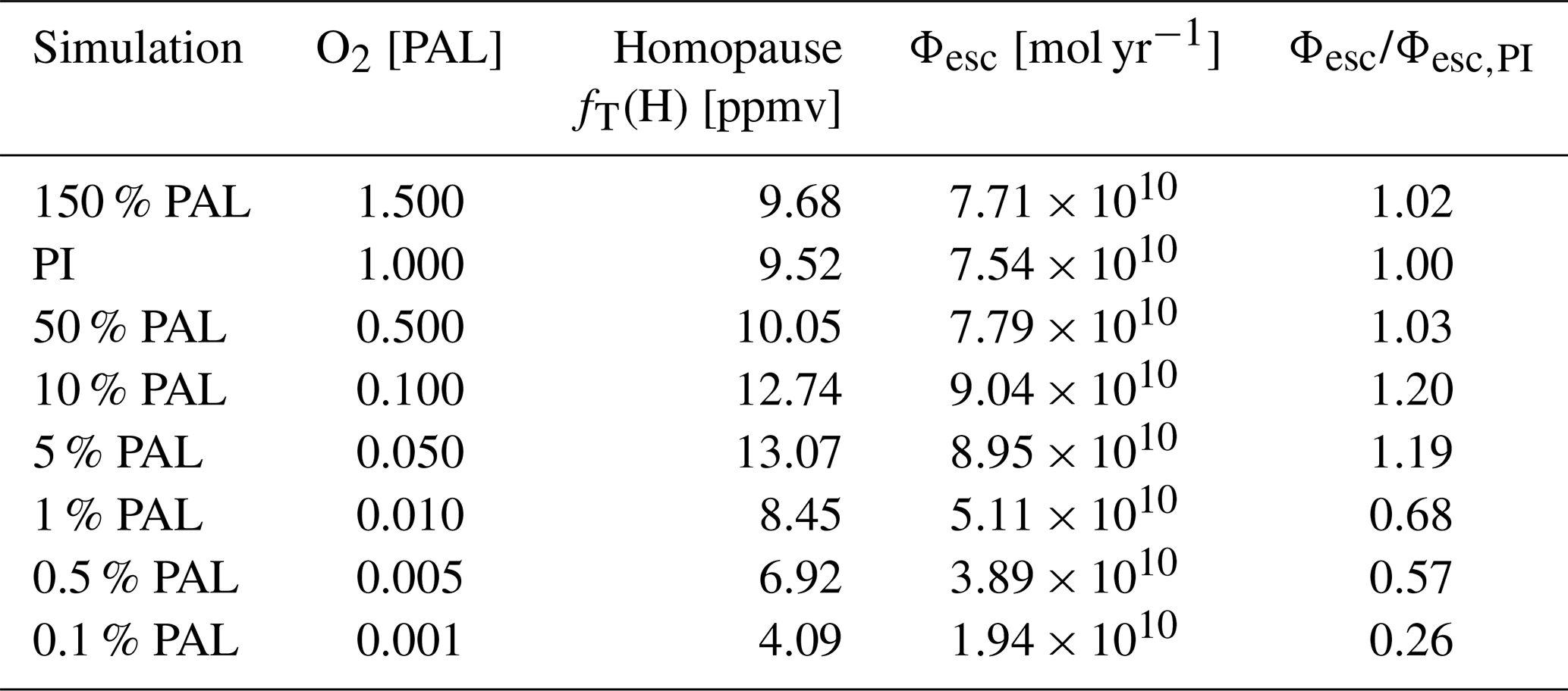
The f_T(H) profile shows that for the cases with ≤ 1 % PAL of O₂, the rate of hydrogen escape is lower than that found in the PI case (Φ_esc,PI). The rates for the 0.1 % PAL, 0.5 % PAL, and 1 % PAL simulations are: 0.26 Φ_esc,PI, 0.57 Φ_esc,PI, and 0.68 Φ_esc,PI, respectively. We also predict that the escape rate could have been slightly higher when O₂ levels were both greater (e.g. 150 % PAL) and lesser (e.g. 5 %–10 % PAL) than the present day value, with the maximum predicted hydrogen escape rate in the 10 % PAL simulation at 1.20 Φ_esc,PI. This shows that the TTL heating and predicted escape rate has a non-linear behavior with O₂ concentration. Following the Great Oxidation Event, Earth's O₂ levels are thought to have fluctuated between 0.1 % PAL and 150 % PAL, although the precise timings and magnitude of these fluctuations are debated (Catling and Zahnle, 2020; Steadman et al., 2020; Planavsky et al., 2020; Yierpan et al., 2020; Krause et al., 2022; Mills et al., 2023; Xie et al., 2023; Fakhraee and Planavsky, 2024; Stockey et al., 2024), with these fluctuations being due to various physical factors, such as carbonate amassing in the crust (Alcott et al., 2024), and large igneous province volcanism combined with weathering (Luo et al., 2024).

4 Discussion

When the Great Oxidation Event occurred approximately 2.4 billion years ago, O₂ increased by several orders of magnitude in the atmosphere in a time frame of approximately 200 Myr (Gumsley et al., 2017). For the first time, these higher levels of O₂ resulted in the generation of a significant O₃ layer which may have created a stratospheric thermal inversion (Kasting et al., 1985; Segura et al., 2003; Cooke et al., 2022). The O₃ layer provided an additional shield for Earth's surface from ultraviolet radiation. However, the exact thickness of the O₃ layer over geological time is difficult to determine. Many uncertainties exist upon the atmospheric pressure and composition throughout the Proterozoic (Lyons et al., 2014; Steadman et al., 2020; Catling and Zahnle, 2020), as well as there being differences in model predictions under similar assumptions (Way et al., 2017; Cooke et al., 2022; Yassin Jaziri et al., 2022; Ji et al., 2023, 2024). With an oxygenated biosphere, the conditions were set for the evolution of oxygen-dependent animals (Cole et al., 2020) and the eventual colonization of land (Dunn, 2013). Additionally, the GOE may have coincided with the end of relatively high levels of hydrogen escape (Zahnle et al., 2013, 2019). Whether other terrestrial worlds go through a similar path of geological and atmospheric evolution is unknown, although it has been modelled under different conditions and assumptions (Gebauer et al., 2018; Olson et al., 2018a; Ozaki and Reinhard, 2021; Krissansen-Totton et al., 2021; Krissansen-Totton and Fortney, 2022).

Our work represents an initial step towards a quantitative estimate for hydrogen escape since the Proterozoic began 2.4 billion years ago. Overall, our results suggest that hydrogen escape during the Proterozoic could have been between 3.8 times lower and up to 1.2 times greater than the calculated pre-industrial escape rate when accounting for O₂ changes only. The present day loss of hydrogen is insignificant on geological timescales, such that the fluctuations in O₂ from the start of the Proterozoic to the present day likely did not in itself cause substantial levels of hydrogen escape. In what follows, we discuss how our simulations can be used as a platform for future work towards the goal of reconstructing Earth's past atmospheric hydrogen escape.

4.1 The oxygen-ozone valve

When only changing the atmospheric O₂ (and N₂) mixing ratio, as O₂ increases from 0.1 % PAL to 150 % PAL, the total atmospheric O₃ column increases (Cooke et al., 2022). Note that increasing quantities of total O₃ does not always lead to an increase in temperatures in the TTL, because the location of the O₃ abundance peak in the atmosphere, and the magnitude of the peak, can move with O₂ mixing ratio. This effect is illustrated by the greater total hydrogen mixing ratio at the homopause in the 10 % and 5 % PAL cases when compared to the PI case (e.g., see Figs. 1, 6, and 7).

Our work shows that O₂ levels during the Proterozoic may have partially controlled the diffusion-limited flux for hydrogen escape. However, this will depend on several other factors, such as the continental distribution and the Earth's obliquity which can affect atmospheric dynamics and seasonal cycles, respectively. The fainter Sun, the albedo of the Earth through time, and various greenhouse gases (including CH₄) which can act to cool the stratosphere but warm the surface (Lin and Emanuel, 2024), will have also impacted TTL temperatures and hydrogen escape rates. For instance, a cooling of the stratosphere can increase the amount of O₃, just like the current increasing atmospheric content of CO₂ is aiding a possible, albeit complex, recovery of the O₃ layer (Rosenfield et al., 2002; Fahey et al., 2018; Ivanciu et al., 2022; Maliniemi et al., 2021).

There exist estimates of many of these aforementioned variables through Earth's history, but each of them come with uncertainties and vary throughout the Proterozoic. Liu et al. (2025) suggest that the O₃ layer could have been kept at low levels due to protracted atmospheric iodine concentrations throughout the Proterozoic. Atmospheric iodine would destroy O₃ through catalytic cycles (WACCM6 does not currently include iodine in its chemical mechanism). The computed WACCM6 O₃ columns are lower than the baseline estimates from Liu et al. (2025), but when Liu et al. (2025) included substantial atmospheric iodine (e.g. 20× modern marine iodine concentrations that was emitted to the atmosphere), then their O₃ columns are lower than the WACCM6 results. If we incorporated iodine, then this could lead to a reduced rate of predicted hydrogen escape at a given O₂ concentration due to diminished O₃ heating.

4.2 Model limitations

Our atmospheric predictions are relevant for both Earth's past and future climate states. However, this statement comes with several caveats. The moist-adiabatic lapse rate (the rate at which the temperature of a parcel of saturated air decreases with altitude as it rises in the atmosphere under adiabatic conditions), strongly depends on temperature. Thus, the total hydrogen mixing ratio in the troposphere of the Earth is determined by the incoming radiation, albedo, and greenhouse effect. For modern Earth, these parameters are relatively well known. We did not attempt to fully account for all climatic changes since the Proterozoic began; instead, as a first step, we focused on the effect on the escape rate by changing O₂ only. The range of O₂ concentrations we accounted for are relevant to the past 2.4 billion years and are not relevant to the Archean eon (4–2.4 Gyr ago) when molecular oxygen was much lower than present day and Proterozoic (2.4–0.541 Gyr ago) concentrations (Catling and Zahnle, 2020). We remind the reader that WACCM6 is designed for the modern Earth and the current set of simulations do not account for a faster rotation rate in the past (Zahnle and Walker, 1987; Bartlett and Stevenson, 2016; Laskar et al., 2023) or different continental coverage (Mitchell et al., 2021). Additionally, we note that changes to the orbital parameters, rotation rate, or obliquity, may affect the tape recorder signal.

Since Cooke et al. (2022) was published, Ji et al. (2023) showed that absorption of light by H₂O and CO₂ in the S-R bands, as well as scattering in the S-R bands, are increasingly important at lower atmospheric O₂ mixing ratios. The simulations presented in this work do not include either of these treatments. Some WACCM6 simulations (at 10 % PAL, 1 % PAL, and 0.1 % PAL) with H₂O and CO₂ absorption in the S-R bands were included in Ji et al. (2023), and we also ran some simulations with fixed surface fluxes (e.g. for CH₄). Whilst the absolute mixing ratios do deviate when this absorption is included, the effect of changing O₂ on temperature is stronger. In terms of scattering, Ji et al. (2023) showed that it is most important at ≤1 % PAL of O₂. Inclusion of scattering will decrease the total O₃ column and likely result in a cooler TTL region. Again, the conclusion that hydrogen escape can be be modified by O₂ concentrations remains unaffected, especially when the prescribed CH₄ mixing ratio sets a minimum on the hydrogen escape rate because it is not cold-trapped. Nevertheless, future simulations where WACCM6 includes both absorption and scattering in the S-R bands will provide more comprehensive atmospheric calculations.

4.3 Future work for Earth

The different climate states that might have existed throughout the Proterozoic and Phanerozoic³ (0.541 Gyr ago–present day) should be simulated in future work. A hotter troposphere may have existed due to increased amounts of CH₄ or CO₂, or both. In this case, the warmer TTL would have increased hydrogen escape rates by elevating the amount of H₂O reaching the stratosphere. On the other hand, colder temperatures during Earth's glacial periods would cool the tropopause (Graham et al., 2019) and reduce the stratospheric H₂O concentration.

Even with a much colder TTL, CH₄ bypases the control of the oxygen valve or a colder troposphere because CH₄ does not condense in Earth's atmosphere like H₂O. Thus, the Proterozoic and Phanerozoic hydrogen escape rate could have instead been controlled by the CH₄ abundance rather than the O₂ abundance, assuming that its mixing ratio reaching the TTL was greater than half the mixing ratio of H₂O in the TTL – see Eq. (2). The current problem with evaluating this effect is that estimates for Proterozoic CH₄ concentrations vary by several orders of magnitude (Pavlov et al., 2003; Daines and Lenton, 2016; Zhao et al., 2018; Olson et al., 2018a; Laakso and Schrag, 2019; Catling and Zahnle, 2020; Cadeau et al., 2020) and may be greater or lower than the present day mixing ratio. The thinner simulated O₃ columns found from 3D modeling (Cooke et al., 2022; Yassin Jaziri et al., 2022) and updated 1D calculations (Ji et al., 2024), as well as the inclusion of iodine chemistry (Liu et al., 2025), suggest that more UV radiation would have penetrated deeper into the atmosphere for much of the Proterozoic and potentially resulted in lower CH₄ lifetimes at O₂ concentrations of ≤1 % PAL. In this situation, greater surface-to-atmosphere fluxes of CH₄ would have been required to sustain current ∼1 ppmv mixing ratios (such fluxes may not be plausible; Daines and Lenton, 2016; Olson et al., 2016; Laakso and Schrag, 2019), or the higher estimates that some studies suggest in the region of ∼10–100 ppmv (Pavlov et al., 2003; Fiorella and Sheldon, 2017; Zhao et al., 2018; Fakhraee et al., 2019). Closer in time to the present day, CH₄ mixing ratios in the Phanerozoic (0.51 Gyr ago–present day) have been simulated to be between 0.1–12 ppmv (Beerling et al., 2009).

Clearly, there is much to still learn about why the different models predict specific atmospheric abundances for molecules such as O₃, which has significant horizontal and vertical variation (Cooke et al., 2022; Yassin Jaziri et al., 2022), and CH₄ (Kasting, 2025). The entire conceivable parameter space has certainly not been fully explored; such endeavors utilising 3D models are welcomed but will likely prove computationally expensive. Attempts to define the CH₄ concentrations in the various geological eons are an important part of the history of hydrogen escape, but for now, the mixing ratio of CH₄ through time remains poorly constrained. Ascertaining its production rate in the Proterozoic will help to establish its concentrations in that eon (Kasting and Ji, 2025).

Eventually, as the Sun's luminosity increases, the Earth will heat up, CO₂ will be sequestered out of the atmosphere through carbonate-silicate weathering, and it is predicted that the Earth will lose all of its water through the moist greenhouse effect approximately 2 Gyr in the future (Kasting et al., 1984; Kasting, 1988; Wolf and Toon, 2014; Ozaki and Reinhard, 2021), although the estimate of the time varies. But before that event occurs, previous studies have predicted that the lack of CO₂ will have a detrimental effect on the biosphere because plants are unable to survive at very low CO₂ concentrations (Lovelock and Whitfield, 1982; Caldeira and Kasting, 1992).

Several calculations of the lifespan of the Earth's biosphere have been attempted (Lovelock and Whitfield, 1982; Caldeira and Kasting, 1992; Franck et al., 2000; Von Bloh et al., 2003; Rushby et al., 2018; Ozaki and Reinhard, 2021; Mello and Friaça, 2023; Graham et al., 2024). For instance, Ozaki and Reinhard (2021) calculated that in 1.08±0.14 billion years (1σ), Earth's atmospheric O₂ will drop to 1 % PAL. More recently, Graham et al. (2024) suggested that Earth's biosphere may last for up to 1.6–1.86 Gyr. Most of these estimates for biospheric termination are before the Earth is predicted to lose its water and become, by the most basic definition, uninhabitable. As O₂ levels drop following the extinction of photosynthesizing life (Ozaki and Reinhard, 2021), O₃ will decrease, and the upper troposphere and TTL may be colder than under otherwise equivalent conditions, diminishing the amount of hydrogen available in the upper atmosphere which can escape to space and cause irreversible water loss (the future rates of hydrogen escape would likely have a negligible effect on oxidizing the Earth to reverse the loss of O₂ from ceasing photosynthesis). Hence, our results suggest that the ocean loss timescale could be extended. Thus, investigations aiming to assess the lifetime of Earth's future habitability should incorporate a 3D chemistry-climate model that includes comprehensive atmospheric oxygen chemistry and that can adequately represent the 3D movement of air parcels through the TTL. Additionally, it is possible that our WACCM6 simulations could be used as input to a model which has a higher top (lower minimum pressure), such as the WACCM-X model (Liu et al., 2018), or even used as an input into a computational model that explicitly calculates atmospheric escape (e.g., Dong et al., 2018; Schulik and Booth, 2023).

4.4 Future work for exoplanets

Other planets outside of our solar system (exoplanets) may be habitable and evolve life. Whether they can keep liquid water on their surface is crucial for the persistence of habitability as it is currently defined.

The H₂O tropical tape recorder is a stratospheric signal of seasonality, impressing the varying TTL temperatures on the stratospheric H₂O mixing ratio. Prior work showed how a 15 % reduction in global O₃ (Xie et al., 2008) could cool the TTL and raise it in height, ultimately weakening the tape recorder signal. Here we find this effect exacerbated further as O₂ and O₃ reduce by orders of magnitude. Transmission spectra of exoplanet atmospheres probe the stratosphere, and whilst beyond the detection limit of today's telescopes, such chemical variability may be detectable with future technology or where exoplanets exhibit higher levels of variation that Earth (e.g., for exoplanets with eccentricity ≥0.4 Liu et al., 2023) or different types of stratospheric variability (Cohen et al., 2022). Seasonality of biosignatures and other gases (Olson et al., 2018b), combined with the H₂O tape recorder signal, may aid in determining whether a planet is inhabited. Should there be no tape recorder signal due to a tropopause that does not significantly vary with seasons, then this variability will be more difficult to observe, and H₂O will be harder to constrain due to a dry middle-upper atmosphere.

Simulations with other 3D models such as the LMD-g (Yassin Jaziri et al., 2022) or the Unified Model (Braam et al., 2022), or those at higher resolutions (e.g., LFRic-Atmosphere; Sergeev et al., 2023), may yield different quantitative results due to varying treatments of convection and water vapour microphysics, as well as alternative radiative transfer schemes. The stratospheric thermal inversion in Earth's atmosphere is due to O₃ which provides sufficient atmospheric heating when O₂ is present in quantities ≳0.1 % PAL (Way et al., 2017; Cooke et al., 2022). But a terrestrial exoplanet may not require O₂ to modulate the thermal structure: other atmospheric compositions can result in thermal inversions and may similarly act to enhance or reduce water loss. For example, Titan has a thermal inversion due to the prescence of hazes which absorb shortwave radiation (Danielson et al., 1973; Catling and Kasting, 2017), and CN on hot super-Earths can also cause a thermal inversion (Zilinskas et al., 2021). Additionally, the heating rates will change depending on the distribution of stellar radiation over wavelengths: O₃ radiative heating significantly affects planets around F and G stars but less so around M and K stars (Godolt et al., 2015; Kozakis et al., 2022; De Luca et al., 2024). O₂ can also build up on exoplanets without the presence of life under specific conditions due to large amounts of CO₂ (Segura et al., 2007) or H₂O photolysis (Wordsworth and Pierrehumbert, 2014).

There are various planetary system parameters which affect the climate state of exoplanets. Crucial to the atmospheric dynamics is the planetary rotation rate and whether it is tidally locked (Forget and Leconte, 2014; Turbet et al., 2016; Boutle et al., 2017; Del Genio et al., 2019b; Braam et al., 2025). The circulation affects the atmospheric temperature structure and how tracers such as H₂O are advected. Other salient factors include the strength and spectral shape of the incoming radiation (Eager-Nash et al., 2020), the continental distribution or lack thereof (Lewis et al., 2018; Zhao et al., 2021; Macdonald et al., 2022), obliquity (Kang, 2019), eccentricity (Liu et al., 2023), flares (Chen et al., 2021; Ridgway et al., 2023), simulation resolution (Sergeev et al., 2020; Lefèvre et al., 2021; Song et al., 2022; Kodama et al., 2022; Yang et al., 2023; Sergeev et al., 2024; Garcia et al., 2024), as well as the planetary Bond albedo and surface composition (Cowan and Agol, 2011; Del Genio et al., 2019a; Madden and Kaltenegger, 2020). Ocean salinity can also be important in modulating the climate of rocky planets (Olson et al., 2022).

By connecting exoplanet simulations to a model that includes the ionosphere (e.g., WACCM-X), one could attempt to answer interesting questions regarding the upper atmospheres of terrestrial exoplanets. For instance, how do the ionospheres of various exoplanets compare to Earth? Just like flares disturb the atmospheres of terrestrial planets (Segura et al., 2010; Tilley et al., 2019; Chen et al., 2021; Ridgway et al., 2023), do flares (especially for active M dwarf stars) impact their ionospheres differently from those that strike the Earth (Leonovich and Tashchilin, 2009; Schillings et al., 2018; Hayes et al., 2021)? And could those differences manifest in a way which is detectable with future instruments (Mendillo et al., 2018; Mendillo, 2019)?

The maximum difference we found in the diffusion-limited hydrogen escape between alternative oxygenation states when all other initial conditions and boundary conditions are kept constant is a factor of 4.7. Whilst this change is not significant for Earth under the assumptions made in this work, it potentially could be significant when the ocean loss timescale for a habitable terrestrial exoplanet is similar to a time that a planet could theoretically spend in the habitable zone (i.e. a planet with a 10 Gyr ocean loss timescale with a different oxygenation state could instead have an ocean loss timescale of ≈2 Gyr).

5 Conclusions

Since the dawn of the Proterozoic (2.4 Gyr ago), several properties of the Earth have changed. The continental configuration has shifted several times, the Sun's luminosity has increased, and the concentration of atmospheric gases such as O₂, CO₂, and CH₄ have fluctuated.

This work used WACCM6 simulations of the Earth to explore the effect that the changing O₂ mixing ratio had on the total hydrogen mixing ratio at the homopause in order to predict the possible diffusion-limited hydrogen escape rate through geological time. A 3D model with chemistry and a global representation of water vapour microphysics is critical to simulating the transport of H₂O into the stratosphere and thus estimating diffusion-limited hydrogen escape when other atmospheric constituents (e.g., CH₄ and H₂, which we held constant at the surface) are not the dominant hydrogen bearing species. In our simulated scenarios we showed that 1D models may predict a stratospheric water vapour discrepancy of between a factor of 3.8–6.0 depending on the O₂ mixing ratio when compared to 3D calculations.

We found that the atmospheric O₂ mixing ratio acts as a nonlinear valve on the total hydrogen mixing ratio in the stratosphere. The O₃ mixing ratio (which is affected by the abundance of O₂) around the tropical tropopause layer (TTL) determines the amount of UV heating that warms the TTL and controls the H₂O mixing ratio entering the stratosphere. The obliquity of Earth induces seasonal cycles, which affect phenomena such as the Brewer-Dobson circulation and the tropical tape recorder. We showed that the tropical tape recorder disappeared at 0.1 % PAL, which suggests that the present-day seasonal transport of H₂O molecules to the stratosphere may not have taken place at low O₂ mixing ratios.

Between 0.1 % PAL and 150 % PAL of O₂, the upward diffusion of H₂O is modulated in a non-linear manner, with 5 % and 10 % PAL having the maximum predicted diffusion-limited escape rate of hydrogen due to O₃ concentrations causing localized heating. The predicted escape rate changes by up to a factor of 4.7 between all of the simulations, meaning that whilst the oxygen valve affects diffusion-limited hydrogen escape, in the absence of other factors, it would not have resulted in relatively high levels of hydrogen escape and thus water loss since the GOE.

In order to dissect Earth's atmospheric history, future work should investigate multiple other physical, chemical, and biological factors that may affect the hydrogen escape rate whilst also accounting for the oxygen valve we presented.