Past Ocean surface density from planktonic foraminifera calcite δ¹⁸O

Density of seawater is a critical property that controls ocean dynamics. Previous works suggest the use of the δ¹⁸O calcite of foraminifera as a potential proxy for paleodensity. However, potential quantitative reconstructions were limited to the tropical and subtropical surface ocean and without an explicit estimate of the uncertainty in calibration model parameters. We developed the use of the δ¹⁸O_c of planktonic foraminifera as a surface paleodensity proxy using Bayesian regression models calibrated to annual surface density. Predictive performance of the models improves when we account for inter-species specific differences.

We investigate the additional uncertainties that could be introduced by potential evolution of the δ¹⁸O_c-density relationship with time – from the last glacial maximum (LGM) to the preindustrial (PI) – through the combination of past isotope enabled climate model simulations and a foraminiferal growth module. We demonstrate that additional uncertainties are weak globally, except for the Nordic Seas region.

We applied our Bayesian regression model to LGM and Late Holocene (LH) δ¹⁸O_c foraminifera databases to reconstruct annual surface density during these periods. We observe stronger LGM density value changes at low latitudes compared to mid latitudes. These results will be used to evaluate numerical climate models in their ability to simulate ocean surface density during the extreme climatic period of the LGM.

The new calibration has great potential to reconstruct the past temporal evolution of ocean surface density over the Quaternary. Under climates outside the Quaternary period and in ocean basins characterized by anti-estuary circulation, like the current Mediterranean Sea and Red Sea, our calibration could provide density estimates with larger uncertainty, a point that requires further investigations.

1 Introduction

Temperature and salinity control the density of seawater and therefore the ocean dynamics too. Reconstruction of past ocean surface temperature with reasonable uncertainties is possible (MARGO Project Members, 2009; Tierney et al., 2020b) but reconstructions of past surface salinity remain very challenging in paleoceanography. When the current uncertainties on past temperature and salinity reconstructions are cumulated, it becomes unreasonable to combine these two parameters in order to quantify past ocean density and dynamics (Schmidt, 1999).

Rather than using the combination of temperature and salinity, previous works suggest the use of the δ¹⁸O of foraminiferal calcite as a potential proxy for paleodensity (Lynch-Stieglitz et al., 1999; Billups and Schrag, 2000, LeGrande et al., 2004; Lynch-Stieglitz et al., 2007). The oxygen isotopic composition of foraminifera calcite is controlled by (1) the temperature dependence of the equilibrium fractionation during calcite precipitation and (2) the isotopic composition of seawater in which the shell grows (Urey, 1947; Shackleton, 1974). Except in areas of sea ice formation or melt, the isotopic composition of seawater (δ¹⁸O_sw) is regionally related to salinity, since they are affected by processes such as evaporation, precipitation, and the water masses advection and mixing (Craig and Gordon, 1965). Therefore, both temperature and δ¹⁸O_sw changes that affect the foraminifera δ¹⁸O calcite (δ¹⁸O_c) signal are also the processes that ultimately define the seawater density in which the foraminifera calcifies (Lynch-Stieglitz et al., 1999; Billups and Schrag, 2000).

In addition to temperature and δ¹⁸O_sw, the shell δ¹⁸O_c signal can also be potentially influenced by biological processes, such as: (1) photosynthesis in algal symbionts (Duplessy et al., 1970; Ravelo and Fairbanks, 1992; Spero and Lea, 1993; Spero et al., 1997) and biases due to the formation of gametogenic or ontogenetic calcite (Williams et al., 1979; Spero and Lea, 1996; Hamilton et al., 2008), (2) changes in pH and carbonate ion concentration [CO${}_{\mathrm{3}}^{\mathrm{2}-}$] (Spero et al., 1997; Bijma et al., 1999; Zeebe, 1999), (3) dissolution and recrystallization for shells deposited in bottom waters undersaturated in [CO${}_{\mathrm{3}}^{\mathrm{2}-}$] (Schrag et al., 1995), and (4) bioturbation (Waelbroeck et al., 2005). The four processes mentioned above have not been clearly demonstrated. In addition, the carbonate ion effect has been shown to have no detectable influence (Köhler and Mulitza, 2024) and core top data have been selected to limit the bioturbation effect (Waelbroeck et al., 2005). Therefore, we do not account for these processes. Transport of foraminifera shells by currents is another process that could lead to discrepancies between recorded δ¹⁸O_c and calculated δ¹⁸O_c or hydrographic data. However, this effect is likely minimal because the ambient water mass is transported together with the shells. Later in this study (Sect. 3.1.2), we confirm that planktonic foraminifera δ¹⁸O_c is mainly related to the surface ocean density, growth season and habitat depth, with weak additional influence from biological processes.

Previously, Billups and Schrag (2000) used δ¹⁸O_c from the mixed layer planktonic foraminifera (Globigerinoides ruber and Trilobatus sacculifer) as a proxy of surface water density. They limited their study to the tropical and subtropical surface ocean.

In this study we investigate the use of planktonic foraminifera δ¹⁸O_c as a surface paleodensity proxy for the whole ocean, from low to high latitudes, using various foraminifera species: Globigerinoides ruber (G. ruber), Trilobatus sacculifer (T. sacculifer), Globigerina bulloides (G. bulloides), Neogloboquadrina incompta (N. incompta), and Neogloboquadrina pachyderma (N. pachyderma). Compared to Billups and Schrag (2000), we use extended late Holocene (LH) and last glacial maximum (LGM) δ¹⁸O_c databases (Malevich et al., 2019; Caley et al., 2014; Waelbroeck et al., 2014a; Tierney et al., 2020b). We develop mean annual surface density calibration models using a Bayesian approach. We also use numerical climate simulations obtained with isotope enabled climate models (iLOVECLIM and ECHAM5/MPI-OM) and a foraminiferal growth module (FAME) (Roche et al., 2018) to investigate the specific seasonal dynamic and depth habitat preference of foraminifera (Roche et al., 2018; Schiebel and Hemleben, 2017). We discuss the applicability and validity of the foraminifera δ¹⁸O_c to the past quantification of surface ocean density. We then reconstruct past surface density changes during the LGM.

2 Methods

2.1 Planktonic foraminifera δ¹⁸O databases

We compiled global foraminifera oxygen isotopic datasets from published LH and LGM measurements to allow reconstruction of past density. We used core-top and LH records of planktonic foraminifera δ¹⁸O_c from Malevich et al. (2019) dataset that include records from the Multiproxy Approach for the Reconstruction of the Glacial Ocean (MARGO) (Waelbroeck et al., 2005) with additional sources. This dataset consists of 2636 observations with 1002 for G. ruber, 635 for G. bulloides, 442 for T. sacculifer, 132 for N. incompta and 425 for N. pachyderma (Malevich et al., 2019). Similarly to Malevich et al. (2019), we gridded the core-top data to reduce the impact of spatial clustering by averaging samples for each species to the nearest 1°×1° grid point. So doing, we obtained a total of 1415 grid points.

For the LGM time period, records derived in part from the MARGO collection (Waelbroeck et al., 2014a), with additional data from Caley et al. (2014), Tierney et al. (2020b), and from more recent studies (34 measurements). The final dataset consists of 474 observations. Chronostratigraphic quality for the LGM and LH is consistent between all the published databases, the additional observations and use the same MARGO definition (MARGO Project Members, 2009).

2.2 Ocean dataset

In order to establish and test our calibrations between foraminifera δ¹⁸O_c and observed surface density, we used different ocean datasets. We used the Multi Observation Global Ocean Sea Surface density product for our core-top and Late Holocene calibration models (Droghei et al., 2016, 2018a). This means that we calibrated Late Holocene core-top samples against observed density fields influenced by anthropogenic climate change, an issue that affects all core-top calibrations. To test the residual of our models against sea surface temperature and salinity (SST and SSS respectively) we used WOA18 products (Locarnini et al., 2018; Zweng et al., 2018).

2.3 Bayesian calibration models and evaluation

Following the general approach of Malevich et al. (2019), we use Bayesian regressions to model the relationship between the calcite oxygen isotopic composition of planktonic foraminifera, δ¹⁸O_c (‰ VPDB), and annual mean surface density, ρ (kg m⁻³ relative to the water density of 1000 kg m⁻³). By explicitly estimating uncertainty in the calibration model parameters, each model produces a full posterior predictive distribution for the predictant ρ. We implement three Bayesian models – two pooling models with first- and second-degree polynomials, and a hierarchical first-degree polynomial model – using Markov chain Monte Carlo (MCMC) methods (see Kruschke, 2014; McElreath, 2018 for review).

2.3.1 Three Bayesian calibration models

1. First-Degree Polynomial (Pooled), poly1_pool: a simple linear regression is fit to all foraminifera species combined:

   $$\begin{array}{}\text{(1)}& \mathit{\rho }\sim N\left(\mathit{\mu },{\mathit{\sigma }}^{\mathrm{2}}\right),\mathit{\mu }={\mathit{\beta }}_{\mathrm{0}}+{\mathit{\beta }}_{\mathrm{1}}{\mathit{\delta }}^{\mathrm{18}}{\mathrm{O}}_{\mathrm{c}}.\end{array}$$

   Weakly informative data-adaptiv normal hyperpriors are used for β₀ and β₁, and an exponential prior for the noise term sigma. This pooled model assumes a common relationship across all foraminifera species (see Appendix A).

2. Second-Degree Polynomial (Pooled), poly2_pool: motivated by empirical evidence (e.g., Billups and Schrag, 2000), the second model incorporates a quadratic term:

   $$\begin{array}{}\text{(2)}& \mathit{\rho }\sim N\left(\mathit{\mu },{\mathit{\sigma }}^{\mathrm{2}}\right),\mathit{\mu }={\mathit{\beta }}_{\mathrm{0}}+{\mathit{\beta }}_{\mathrm{1}}{\mathit{\delta }}^{\mathrm{18}}{\mathrm{O}}_{\mathrm{c}}+{\mathit{\beta }}_{\mathrm{2}}{\left({\mathit{\delta }}^{\mathrm{18}}{\mathrm{O}}_{\mathrm{c}}\right)}^{\mathrm{2}}.\end{array}$$

   Again, we apply weakly informative normal priors for the β_i parameters, ensuring flexibility while constraining the plausible range based on the observed data.

3. First-Degree Polynomial (Hierarchical), poly1_hier: the third model recognizes that species-specific differences in calcification, depth, seasonality and vital effects can affect δ¹⁸O_c (Malevich et al., 2019). Hence, we use a hierarchical structure:

   $$\begin{array}{}\text{(3)}& \mathit{\rho }\sim N\left({\mathit{\mu }}_{\mathrm{s}},{\mathit{\sigma }}_{\mathrm{s}}^{\mathrm{2}}\right),{\mathit{\mu }}_{\mathrm{s}}={\mathit{\beta }}_{\mathrm{s},\mathrm{0}}+{\mathit{\beta }}_{\mathrm{s},\mathrm{1}}{\mathit{\delta }}^{\mathrm{18}}{\mathrm{O}}_{\mathrm{c}}\end{array}$$

   where each species s has its own intercept (β_s,0) and slope (β_s,1). These species-level parameters are drawn from common hyperdistributions ν_i and κ_i (Appendix A), ensuring partial pooling of information across species.

2.3.2 Model fitting and evaluation

All models were fitted with six independent MCMC chains of 4000 iterations each, discarding the first 2000 as burn-in. We used rank-normalized $\widehat{R}$ (Vehtari et al., 2021) to assess convergence, finding all values below 1.05. Prior and posterior predictive checks confirmed the adequacy of the models. To compare predictive performance, we computed the expected log pointwise predictive density (ELPD) via Pareto-smoothed importance sampling leave-one-out cross-validation (LOO) (Vehtari et al., 2017), which provides a principled basis for selecting the model that best characterizes the relationship between δ¹⁸O_c and ρ. The ELPD measures the expected predictive accuracy of a Bayesian model. It is defined as the sum over all data points of the expected log posterior predictive density (Gelman et al., 2014). In our case, a higher ELPD means the model makes sharper and more accurate density predictions.

2.4 Isotope enabled numerical climate models

2.4.1 The iLOVECLIM model

The iLOVECLIM (version 1.1.3) earth system model of intermediate-complexity is a derivative of the LOVECLIM-1.2 climate model extensively described in Goosse et al. (2010). From the original model, we retain the atmospheric (ECBilt, resolution of 5.6° in latitude and longitude), oceanic (CLIO, 3×3° horizontal resolution, 20 vertical layers and a free surface), vegetation (VECODE) and land surface (LBM) components and develop a complete, conservative, water isotope cycle through all cited components. A detailed description of the method used to compute the oxygen isotopes in iLOVECLIM can be found in Roche (2013) and the validation of model results can be found in Roche and Caley (2013), Caley and Roche (2013) and Extier et al. (2024).

We use the boundary conditions defined in/by the PMIP2 protocol to simulate the annual LGM climate (Caley et al., 2014). Details about the model simulations – LGM and pre-industrial (PI) – and validation of results for oxygen stable isotopes and temperature can be found in Caley et al. (2014).

2.4.2 The ECHAM5/MPI-OM model

We also use the ECHAM5/MPI-OM coupled General Circulation Model (GCM), also previously named community Earth system model COSMOS. It is a fully coupled ocean–atmosphere–sea ice–land surface model (Jungclaus et al., 2006) with stable water isotope diagnostics in all relevant model components. Mass, energy, and momentum fluxes, as well as the related isotope masses of H${}_{\mathrm{2}}^{\mathrm{18}}$O and HDO, are exchanged between the atmosphere and ocean once per day. Further details about the model can be found in Werner et al. (2016).

We used monthly outputs of the two simulations performed for the PI and for the LGM climate as described and evaluated for oxygen stable isotopes in Werner et al. (2016).

2.5 The FAME module

Foraminifera as Modelled Entities (FAME; Roche et al., 2018) is a foraminiferal growth module that tackles the dynamic seasonal and depth habitat of planktonic foraminifera. The module predicts the presence or absence of commonly used planktonic foraminifera and their δ¹⁸O values. It uses a very limited number of parameters, almost all derived from culture experiments (Lombard et al., 2009).

3 Results and discussion

3.1 Ocean surface density from planktonic foraminifera calcite δ¹⁸O

The three Bayesian calibration models reasonably replicate core top data spread when we predict surface density (Fig. 1).

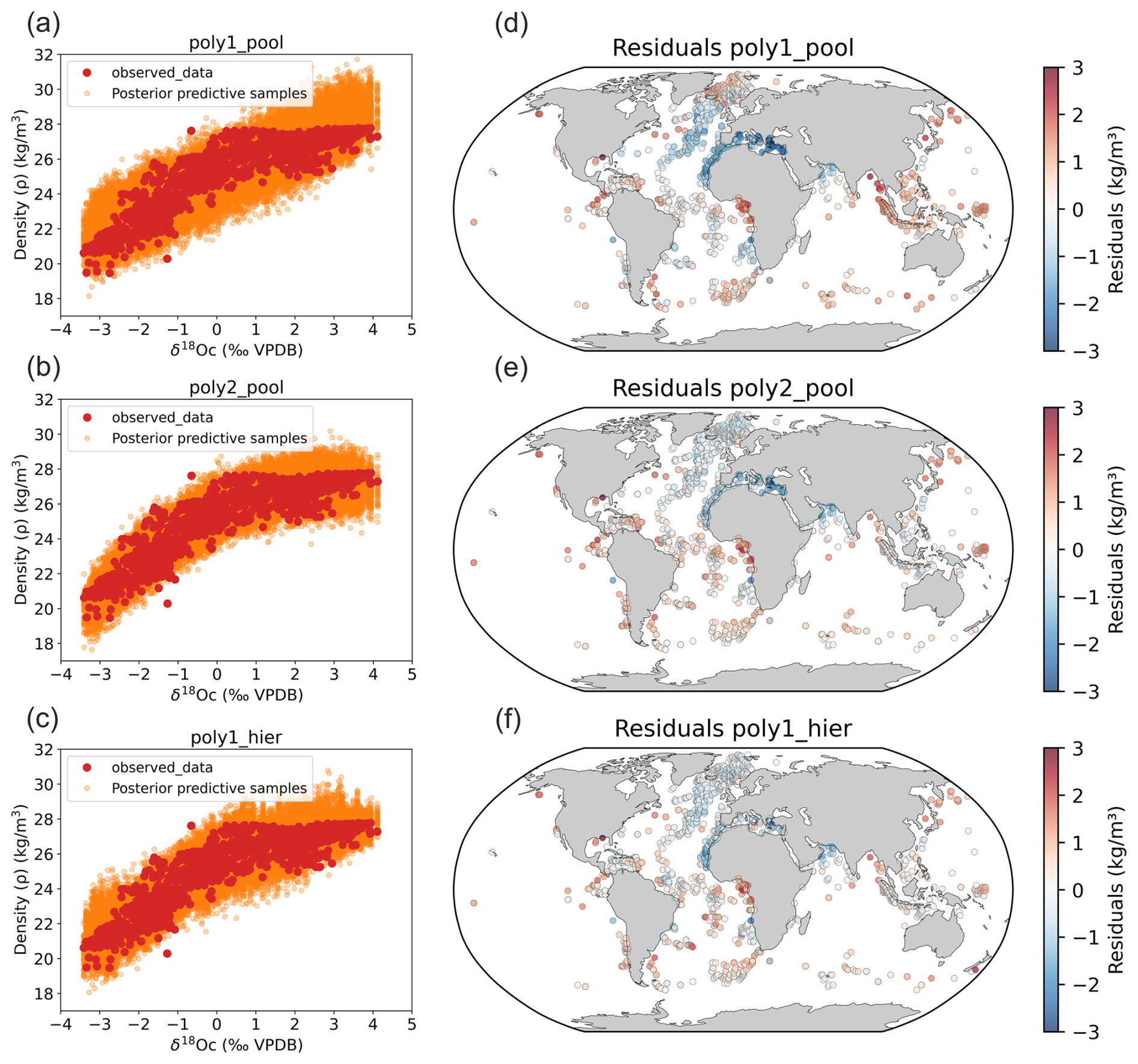
Figure 1 Bayesian calibration models for late Holocene core-top samples against observed density. (a–c) The three Bayesian regression models between foraminifera δ¹⁸O_c and annual surface density and (d–f) associated density residuals (predicted–observed).

Compared to the Billups and Schrag (2000) study which was restricted to the 21–26 density range in tropical and subtropical regions, our models provide estimates of the density changes over the whole density range from 19 to 28 (Fig. 1). In our new calibrations, we also explicitly estimate the uncertainty in calibration model parameters (Fig. 1) using a Bayesian approach to calculate robust confidence intervals.

We observe a saturation of density values close to 28 in the calibrations that correspond to high latitudes regions (Nordic Seas and Austral Ocean). When density is already high, temperature changes have a smaller effect. Cold water is already dense, so cooling it further does not increase density as much. Consequently, we observe a sensitivity decrease. The rate of change of density with respect to temperature flattens out, meaning that the system becomes less responsive to temperature changes. Small changes in temperature and salinity no longer cause significant shifts in density. This behavior reflects to the non-linearity of the seawater equation of state. Although the regression becomes less predictive in this range, the estimated density values remain correct and are not expected to change strongly as ocean surface density approaches its upper limits.

3.1.1 Model comparison and residuals

Looking at the density residual (predicted–observed) for the three models, the first model (linear pools) has the highest values of residual and the third model (hierarchical design) performs best (Fig. 1). The second model performs clearly better than the first one but less than the hierarchical design. This is supported by model evaluation using log pointwise predictive density (ELPD) (Vehtari et al., 2017) (Fig. 2). Predictive performance of the model improves when we account for species-specific differences and species-specific prediction uncertainty (sigma) in surface density predictions vary between foraminifera species (Fig. 2).

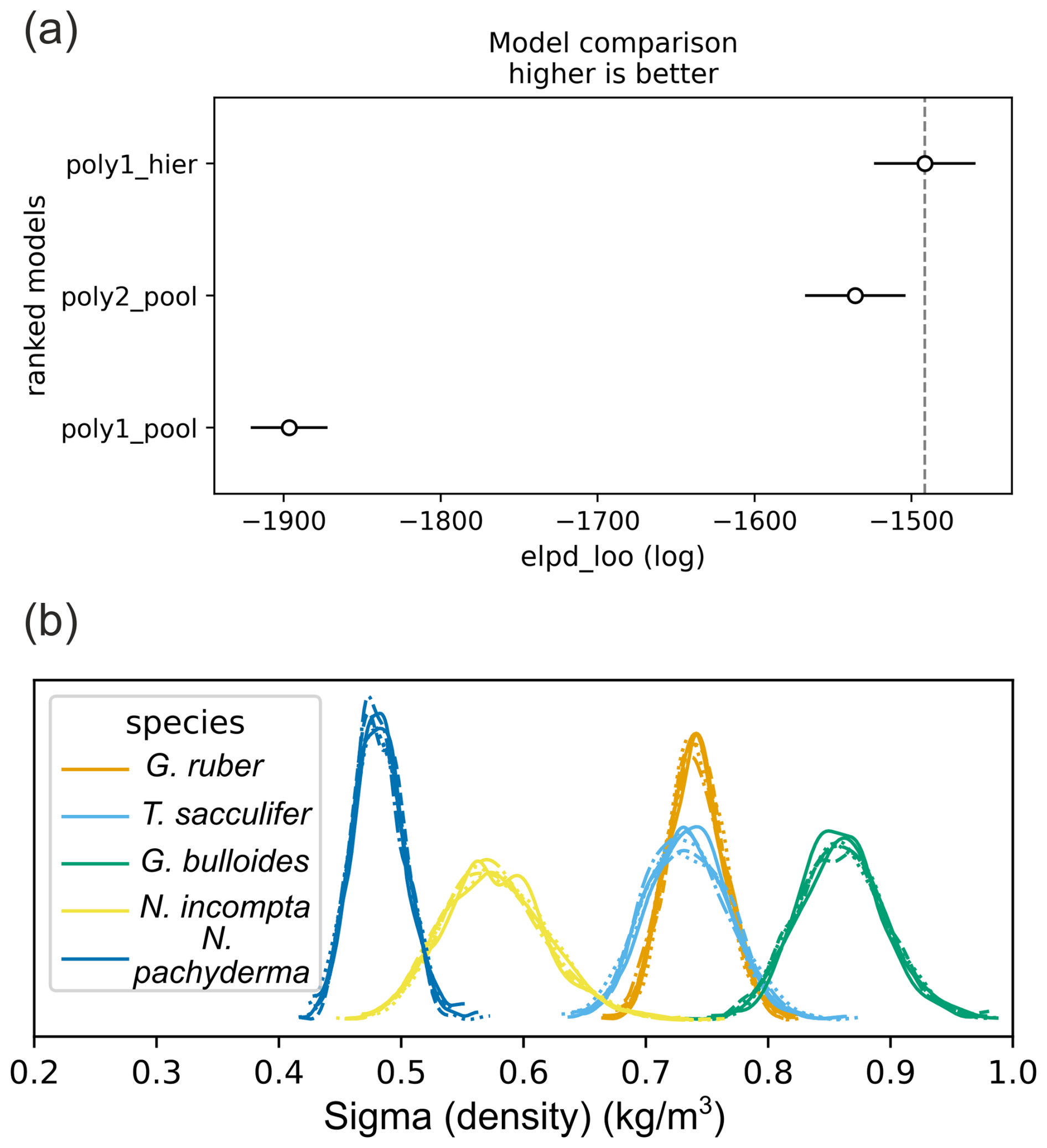
Figure 2 Model comparison and prediction uncertainty across species. (a) Expected log pointwise predictive density (ELPD) for the three models; higher values indicate better predictive performance. (b) Posterior distributions of the prediction-error parameter (sigma density) from the hierarchical model for each foraminifera species (six MCMC chains shown). Among these, N. pachyderma exhibits the lowest uncertainty, while G. bulloides shows the highest.

We still observe residuals with the hierarchical model (Fig. 1), so we checked their relation to SST and SSS (Fig. 3). The residuals of the pooled linear annual calibration model exhibit a relationship with SST and a linear relationship with SSS with a relatively high correlation (R²=0.55, p value < 0.05). In contrast, the residuals of the hierarchical annual calibration model show no correlation to SST (R²=0, p value < 0.05) and only a very weak correlation with SSS (R²=0.21, p value < 0.05). This suggests that factors other than SST and SSS influence the remaining residual structures, and some may be indirectly associated with SSS gradients. Indeed, ecological factors (e.g. seasonality and habitat depth) and secondary environmental parameters (e.g. nutrients and light penetration) may also contribute. This is supported by the fact that the residual of individual species (Fig. 3) show various significant relations (p value < 0.05) with SSS, with R² values of 0.17 for G. ruber, 0.12 for T. sacculifer, 0.54 for G. bulloides, 0.15 for N. incompta, and 0.32 for N. pachyderma. For example, negative residuals are observed in the Benguela, Canary, Peru and North Arabian regions (Fig. 1). All these coastal areas correspond to upwelling systems and previous work already suggested that foraminifera species could have a preference for nutrient-rich waters with high turbidity. This is particularly true for the seasonal specie G. bulloides (Peeters et al., 2002; Gibson et al., 2016). The δ¹⁸O_c may therefore be biased toward colder temperatures even when accounting for seasonality and species-specific sensitivity (Malevich et al., 2019). This could explain why all three models yield lower densities than the observed annual mean densities in the upwelling zones. The negative density residuals in these upwelling regions may reflect this habitat preference (Fig. 1).

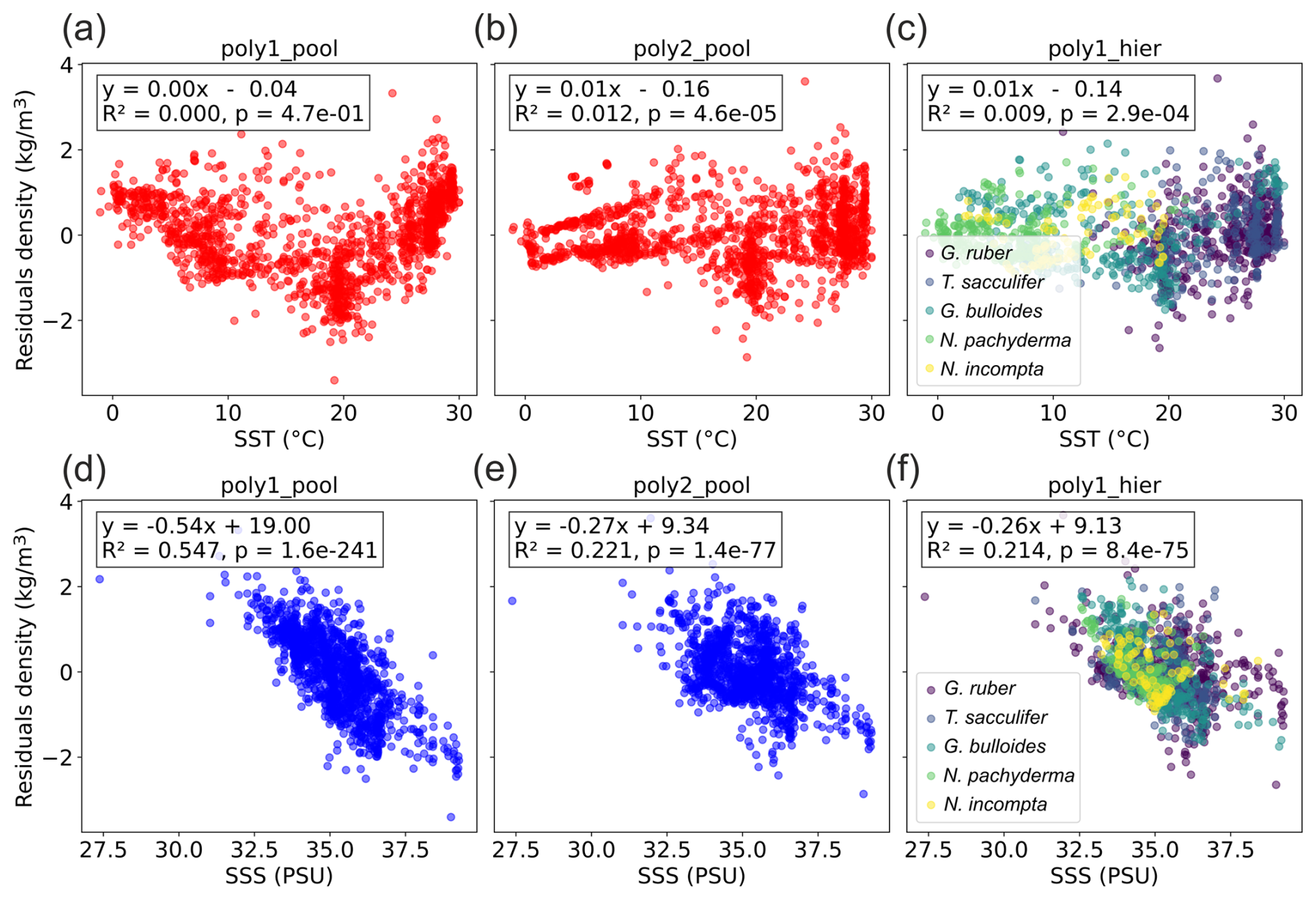
Figure 3 Relation between density residuals (predicted–observed) and (a–c) SST and (d–f) SSS (WOA18 products, Locarnini et al., 2018; Zweng et al., 2018) for the three Bayesian regression models. R² and p values are indicated.

Strong negative residuals are also observed in the eastern part of the Mediterranean Sea. Malevich et al. (2019) reported reduced performance of their hierarchical seasonal calibration model for δ¹⁸O_c and SST in this region and attributed it to the unusual behavior of G. ruber, potentially linked to depth-habitat migration. But estimation of seasonality for this region could also be problematic and play a role as highlighted in the study of Ayache et al. (2024). Alternatively, biases in Mediterranean net freshwater fluxes and thermohaline circulation could affect late Holocene δ¹⁸O_c values (Ayache et al., 2024). Future modelling developments, such as the use of high-resolution regional model in combination with the FAME module, could help to better understand the relation between δ¹⁸O_c, density, temperature and δ¹⁸O_sw during past climate changes in the Mediterranean Sea.

We also observe high positive residual values in the Equatorial and South Atlantic Ocean, in particular on the equatorial African margin and to a lesser degree in the Equatorial East Pacific Ocean. As discussed later (Sect. 3.1.2), these positive density residuals could be related to ecological factors such as seasonality.

It is possible to take into account seasonality based on an estimation of foraminiferal seasonal abundance (Malevich et al., 2019), or using the FAME module. This module predicts the mean δ¹⁸O_c of a foraminifera sample constituted of a number of individuals by weighting in space (depth in the water column) and time (months) the oceanic conditions by the growth rate of each individual.

We decided to not directly develop seasonal calibration models for several reasons. First, we want to predict annual surface density to be able to compare and evaluate numerical climate models against annual surface density. Second, including seasonal signals in foraminifera in our Bayesian models using sediment trap data (Malevich et al., 2019) or seasonality and habitat depth using FAME (that uses the temperature dependence of growth derived from culture experiments (Lombard et al., 2009)) would be a simplification that does not consider factors such as light and nutrient availability. Third, even if it could potentially improve the models for the present day calibration, although a hierarchical seasonal model does not necessary show an increase in validation performance compared to the hierarchical annual model (Malevich et al., 2019), this approach assumes that seasonality or habitat depth would not change during past periods. Results using FAME demonstrate that seasonality or habitat depth change during past periods (Roche et al., 2018). Therefore, changes in seasonality and habitat depth could introduce additional uncertainties when using a seasonal calibration model to predict past seasonal surface density. One possibility would be to use simulation results for past periods to force the FAME module and create past Bayesian calibration models between δ¹⁸O_c and surface density that would take into account ecological changes. However this would not be independent of climate models and would lead to circular reasoning if the purpose is to use reconstructed density for comparison and evaluation of past climate simulations.

We therefore adopt a different strategy. We use past isotope enable climate model simulations for the pre-industrial (PI) and LGM periods to force the FAME module in order to test within the “model world” if a PI Bayesian calibration (hierarchical design) between the δ¹⁸O_c and annual surface ocean density is stable with time and if the changes in foraminifera growth season and habitat depth lead to additional uncertainties when applying a PI relation to past annual predictions (LGM).

3.1.2 Testing the stability of the δ¹⁸O_c–density relation during past periods

Because the proposed approach to reconstruct ocean surface density uses the temperature and δ¹⁸O_sw influence on the δ¹⁸O_c signal, we investigated the potential evolution of the δ¹⁸O_c–density relationship with time before applying this approach to past density reconstructions. In particular, we investigated two questions: does the present day δ¹⁸O_sw–salinity relationship and its known past temporal evolution (Rohling, 2000, LeGrande and Schmidt, 2011, Caley and Roche, 2015) significantly affect the density–δ¹⁸O_c relation evolution? Do ecological changes (foraminifera growth season and habitat depth) significantly affect the density–δ¹⁸O_c relation evolution?

We use numerical climate simulations (LGM and PI) of two isotope enabled numerical climate models, iLOVECLIM and ECHAM5/MPI-OM, to address these questions. We calculate the δ¹⁸O_c signal based on the simulated δ¹⁸O_sw and ocean temperature for both PI and LGM using the quadratic approximation of Kim and O'Neil (1997) given in Bemis et al. (1998). We use the FAME module to predict the δ¹⁸O_c values and account for foraminifera specific living habitats in the water column and along the year as described in Roche et al. (2018). A comparison of the simulated and observed core-top data δ¹⁸O_c (Fig. 4) shows high correlation (R² of 0.93 and 0.89 for ECHAM5/MPI-OM and iLOVECLIM respectively). The slightly higher correlation with ECHAM5/MPI-OM and associated lower root mean square error (RMSE) (Fig. 4) could be related to differences in climate models but also to the fact that in the chosen configuration iLOVECLIM generated only annual δ¹⁸O_sw and ocean temperature hydrographic data contrary to ECHAM5/MPI-OM that produces monthly results. Therefore, the seasonality effect is only simulated by combining FAME and ECHAM5/MPI-OM whereas the habitat depth effect is simulated in both experiments.

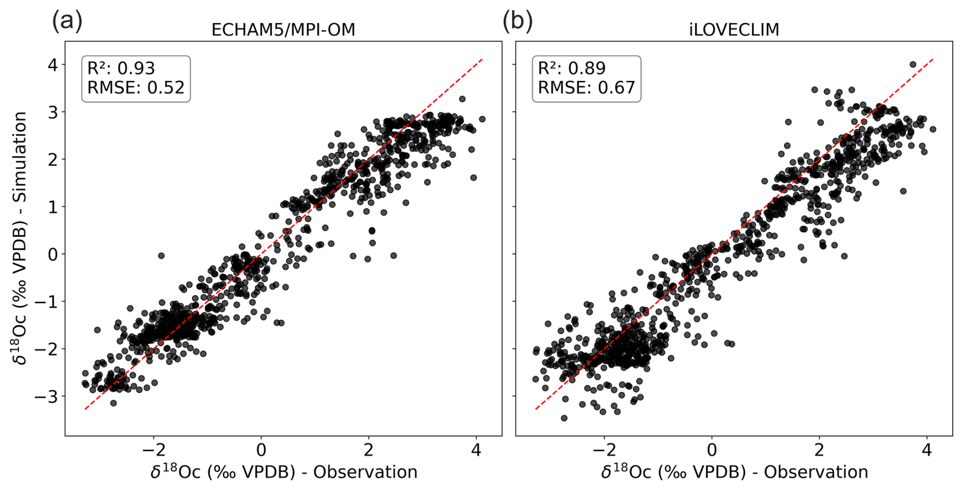
Figure 4 Comparison between simulated PI foraminifera δ¹⁸O_c – FAME module forced with (a) ECHAM5/MPI-OM and (b) iLOVECLIM climate model hydrographic data – and observed LH core-top δ¹⁸O_c data. The 1:1 line is indicated.

We tested this hypothesis by using yearly ECHAM5/MPI-OM values to compute the δ¹⁸O_c and compared the results with those obtained with seasonal values (shown in Fig. 4a) and better assess the effect of seasonality. Results indicate a slight decrease of the R² of 0.02 and a slight increase in RMSE of 0.06 when seasonality is not taken into account. These differences are significant according to paired t tests. Therefore, seasonality partly explains the small difference between the results using ECHAM5/MPI-OM and iLOVECLIM. Lower resolution of iLOVECLIM or other missing/biased processes in this model could also contribute to this small difference.

Although climate models are not perfect, the observed high correlations demonstrate that (1) these numerical climate models can be used to address our questions regarding the stability of the δ¹⁸O_c–density relation during the past and (2) our hypothesis that planktonic foraminifera δ¹⁸O_c is mainly related to the surface ocean density, growth season and habitat depth, with weak additional influence by biological processes (Sect. 1) is valid.

We developed two PI Bayesian calibrations (hierarchical design) between the δ¹⁸O_c and annual surface ocean density based on FAME forced by ECHAM5/MPI-OM and iLOVECLIM hydrographic data (Fig. 5a). These Bayesian calibration models are comparable to the poly1_hier Bayesian calibration model of Fig. 1. We then used the LGM simulations to force FAME and produce δ¹⁸O_c LGM values comparable to those that could be measured in a marine sediment core (but in the model world). We can use these δ¹⁸O_c LGM values and the PI Bayesian calibrations to predict the ocean surface density at the LGM. We can then compare the density reconstructed from the δ¹⁸O_c values to the density simulated directly at the LGM by ECHAM5/MPI-OM and iLOVECLIM. This furnish a test in the model world regarding the stability of the δ¹⁸O_c–density relation during the past.

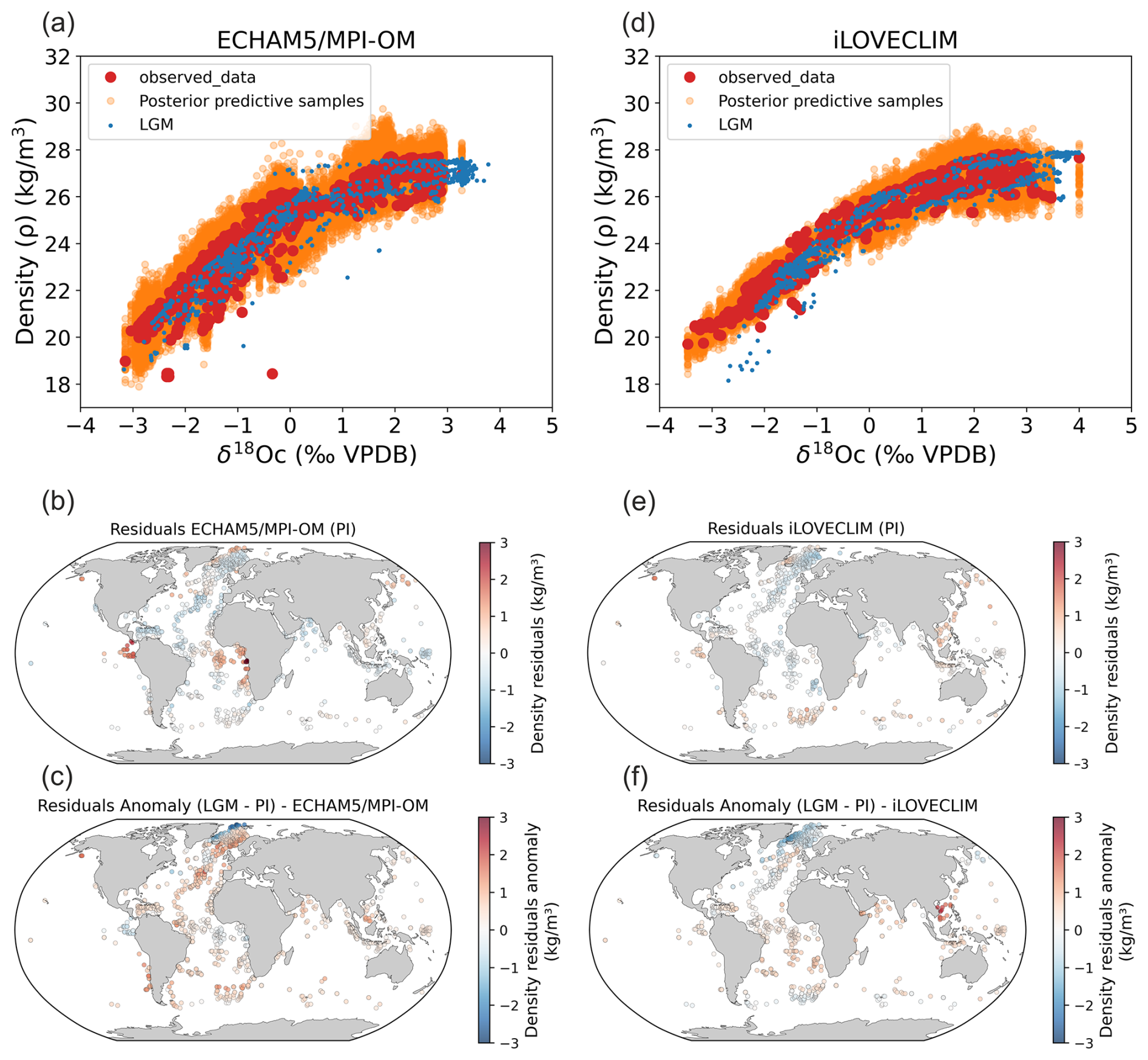
Figure 5 Stability of foraminifera δ¹⁸O_c-density relations between PI and the LGM calculated with FAME and forced by global ECHAM5/MPI-OM (a–c, Werner et al., 2016) and iLOVECLIM (d–f, Caley et al., 2014) hydrographic data. (a, d) PI Bayesian regression models between foraminifera δ¹⁸O_c and annual surface density. Data in the PI experiments have been selected at the same locations as observations (Fig. 1). Posterior predictive samples and the LGM δ¹⁸O_c–density relation (LGM) are visible. (b, e) Density residuals (predicted–observed) for the PI experiments. (c, f) Density residuals anomaly between LGM and PI. Results for the Mediterranean Sea have been excluded because of its difficulty to be simulated and inconsistency between the two model simulations because of their different grid resolutions. Annual mean temperature and δ¹⁸O_sw were used for the iLOVECLIM experiment whereas monthly temperature and δ¹⁸O_sw were used for the ECHAM5/MPI-OM experiment.

Interestingly, the observed (Fig. 1) and simulated (Fig. 5b and e) density residuals (predicted–observed) are overall in good agreement for both PI ECHAM5/MPI-OM and iLOVECLIM experiments in terms of qualitative changes (positive or negative residuals) (Figs. 5b, e and 1). Nonetheless, differences for some regions in terms of magnitude of the residual values exist between ECHAM5/MPI-OM and iLOVECLIM experiments. We observe high positive residuals in the Equatorial and South Atlantic Ocean in the ECHAM5/MPI-OM experiment, in particular on the equatorial African margin and in the Equatorial East Pacific Ocean. As discussed before (Sect. 3.1.1), these positive density residuals are also visible in the observations (Fig. 1f). We attribute these high positive residuals in ECHAM5/MPI-OM (Fig. 5b) that better fit the observations (Fig. 1f) to a seasonality effect because seasonality is only taken into account in ECHAM5/MPI-OM experiment. Negative residuals previously discussed in upwelling regions are visible in simulated residuals but with lower magnitude in comparison to observations (Figs. 1f and 5b, e). This could be related to the fact that upwellings are not well simulated in the two experiments or to the role of secondary environmental parameters such as nutrients and light penetration.

We apply the PI annual Bayesian calibration to the simulated LGM δ¹⁸O_c after a correction of 1.0 ‰ of LGM δ¹⁸O_sw values (value added at LGM for the ECHAM5/MPI-OM and iLOVECLIM experiments, Caley et al., 2014; Werner et al., 2016) to account to a change of the global oceanic δ¹⁸O_sw signal due to the increased LGM ice sheets. This yields a prediction of the LGM surface ocean density that we can compare to the directly simulated LGM surface density in both experiments. We calculate the density residual at the LGM (density reconstructed from the δ¹⁸O_c values – density simulated directly at the LGM). Finally, we calculate the density residuals anomaly between LGM and PI as: density residuals at LGM - density residuals at PI (Fig. 5c and f). This allows us to investigate the additional uncertainties linked to the evolution of the density–δ¹⁸O_c relation (Fig. 5c and f).

The surface density residuals anomalies (LGM–PI) are overall rather close to 0 except in the Nordic Seas region (north of 40° N in the Atlantic). For the following analyses we do not consider the North Indian Ocean for iLOVECLIM. Indeed, this region is affected by a well-known bias of this climate model due to a shift of the African precipitation regions from the west to the east of the continent, leading to much less saline waters than presently observed (and unrealistically depleted δ¹⁸O_sw) in the North Indian Ocean (Roche and Caley, 2013). Higher residuals anomaly in Nordic Seas region could be associated with difficulty in simulating the δ¹⁸O_sw–salinity relation evolution related to ice-sheets and sea ice changes and/or to foraminifera ecological changes between LGM and PI. We also observe in this region larger surface density residuals anomalies (LGM–PI) with ECHAM5/MPI-OM than with iLOVECLIM (Fig. 5c and f). This can be explained by different simulated sea ice coverage in ECHAM5/MPI-OM compared to iLOVECLIM. Indeed, the Nordic Seas is the region with the largest difference between the two model simulations of modeled annual SST below 0 °C (https://doi.org/10.5194/egusphere-2025-2459-AC2, Caley et al., 2025a). Temperature is used to calculate the δ¹⁸O_c signal, ocean density and to force the FAME module. Any temperature difference in the Nordic Seas thus affects density reconstructions and hence the density residuals (Fig. 5c and f).

To further investigate in a more quantitative way if the use of the PI bayesian calibration to predict LGM surface density introduces additional uncertainties, we compare probability distributions of surface density residuals anomaly (LGM–PI) using violin and box plots to the 95 % confidence interval (CI) of the PI bayesian calibration (Fig. 6). We consider each foraminifera species separately. Global results indicate for the G. ruber and T. sacculifer species that (1) the 5th to 95th percentile and interquartile range of the surface density residuals anomaly is well inside the 95 % CI of the PI bayesian calibration for both ECHAM5/MPI-OM and iLOVECLIM experiment and (2) high probability and median values are close to 0 (Fig. 6a and c). This is not the case for G. bulloides, N. incompta, and for N. pachyderma.

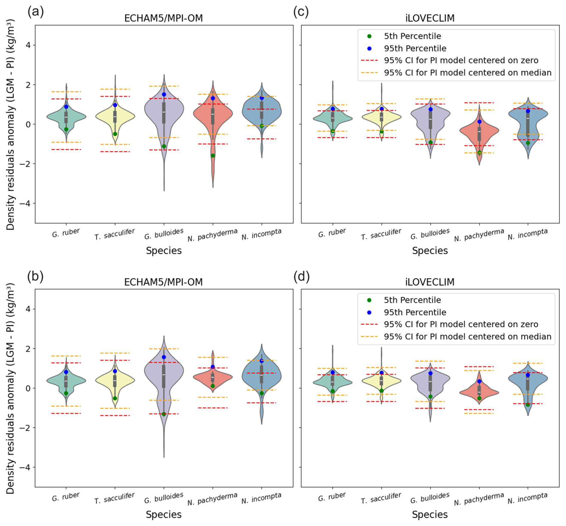
Figure 6 probability distributions of surface density residuals anomaly (LGM–PI) for ECHAM5/MPI-OM and iLOVECLIM, for global data (a, c), and without the Nordic Seas and northern North Atlantic (north of 40° N) (b, d). North Indian Ocean data for iLOVECLIM have been removed in both cases.

When the Nordic Seas region is removed, results indicate that for all the foraminifera species, the interquartile range of the surface density residuals anomaly is well inside the 95 % CI of the PI bayesian calibration for both experiments (ECHAM5/MPI-OM and iLOVECLIM). High probability and median values are closest to 0 (Fig. 6b and d). The 95 % CI of the PI bayesian calibration is closest to the 5th to 95th percentile range of the surface density residuals anomaly.

We conclude based on our tests that the use of a Bayesian calibration model (hierarchical design) to predict annual surface density during past periods (with the example here of the LGM climate) is valid globally within the explicitly estimated uncertainty in calibration model parameters, except for the Nordic Seas region.

3.2 Reconstruction of past ocean surface absolute density

To reconstruct past ocean surface absolute density based on foraminifera δ¹⁸O_c values that have been corrected from the δ¹⁸O_sw ice effect, an additional correction is necessary. Indeed, it is necessary to account for mean ocean density changes related to ocean volume changes that affect mean ocean salinity. Without this additional correction, the ocean density reconstructed corresponds to density changes linked to hydrographic changes in SST and SSS.

To determine the mean ocean density change related to the change in ocean volume at LGM we used model simulation results (ECHAM/MPI-OM and iLOVECLIM) and added or removed 1 psu salinity (Duplessy et al., 1991) in global salinity outputs. Note that adding 1 psu of salinity at LGM in climate model simulations has only small effects on ocean dynamics. Indeed, the effect is due to the small non-linearity in the sea-ice freezing, hence generating small differences in regions of sea ice and deep water formation. We have tested it in new simulations performed with the iLOVECLIM model and found the dynamical effect of a 1 psu salinity change in the regions we are analyzing to be very small (not shown).

Both model simulations agree and yield a mean ocean salinity effect on density of 0.776 (σ=0.02) for ECHAM/MPI-OM and 0.772 (σ=0.02) for iLOVECLIM. We also performed a calculation to estimate this effect based on observations (reference state based on present day observations and LGM state based on Tierney et al., 2020b for SST and Duplessy et al., 1991 for SSS) and found very consistent results (https://doi.org/10.5194/egusphere-2025-2459-AC1, Caley et al., 2025b).

Therefore, the additional correction that is necessary to reconstruct past ocean surface absolute density at the LGM is estimated to be equal to +0.77 kg m⁻³.

3.3 LGM annual surface density reconstruction

We applied the poly1_hier calibration model to the LGM and LH δ¹⁸O_c foraminifera database, excluding the Nordic Seas region, after subtraction of 1.0 ‰ from LGM δ¹⁸O_c values (Labeyrie et al., 1987; Schrag et al., 1996, 2002; Adkins et al., 2002; Duplessy et al., 2002) in order to reconstruct LGM and LH annual surface density. Absolute LGM annual surface density was calculated by adding 0.77 kg m⁻³ to density changes linked to hydrographic changes in SST and SSS. The benefit of our Bayesian model is the possibility to propagate uncertainty from calibration into predictions of past climate conditions (Fig. 7).

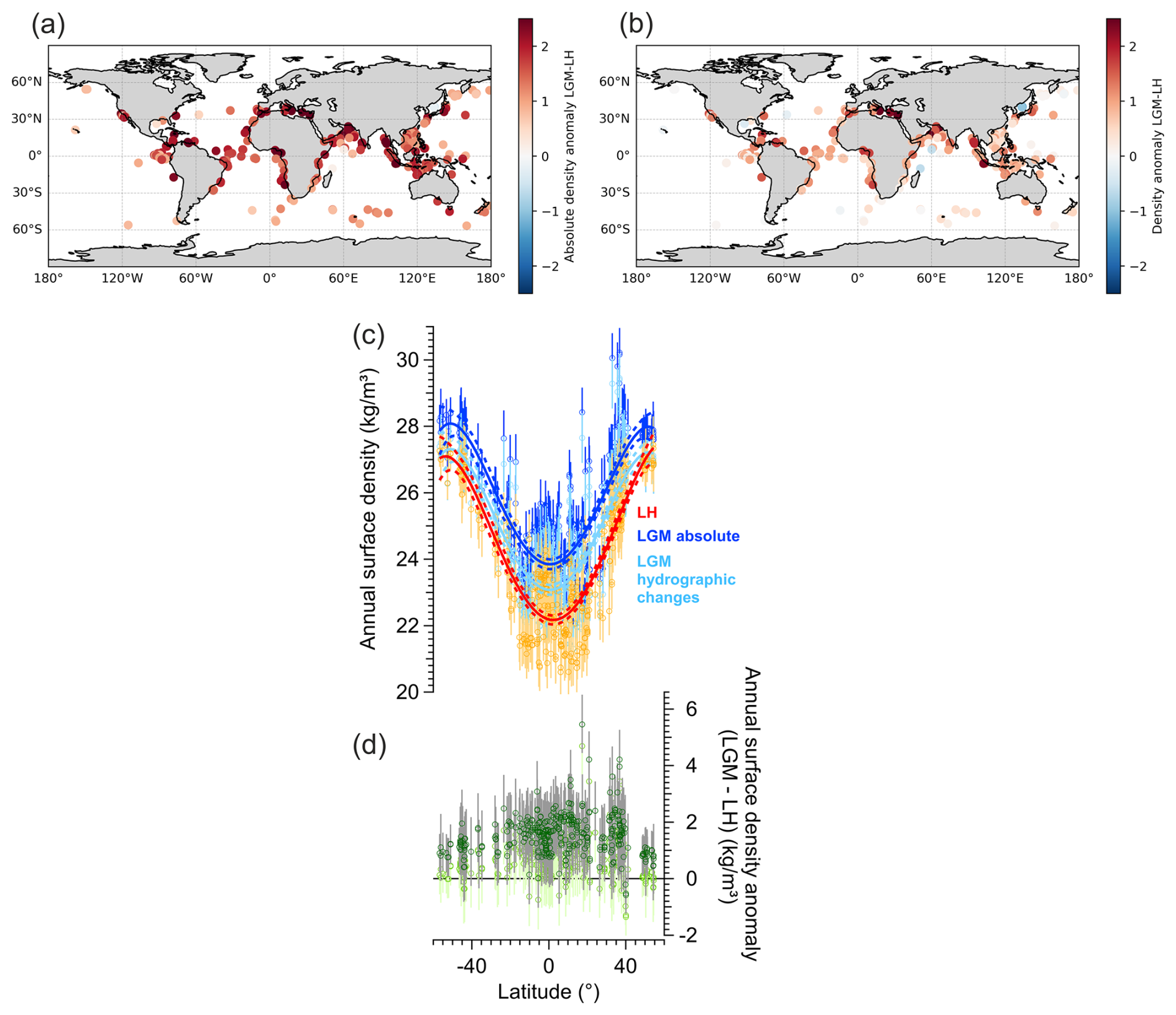
Figure 7 Reconstructions of LGM and LH annual surface ocean density from foraminifera δ¹⁸O_c. (a) Spatial distribution of the LGM–LH absolute density anomaly. (b) Spatial distribution of the LGM–LH density changes due to hydrographic changes in SST and SSS. (c) Meridional gradient of reconstructed surface annual LGM density (absolute density in dark blue, density due to hydrographic changes in light blue) and comparison with LH reconstructions (red and orange colors). Error bars for each data point represent the 68 % CI. A polynomial fit (5th degree) and associated 95 % confidence bands are shown as solid resp. dashed lines. (d) Meridional gradient of reconstructed density anomaly (LGM–LH) for absolute density in dark green and density due to hydrographic changes in light green and associated 68 % CI (grey lines).

Ocean surface density increases globally during the LGM in agreement with colder SST (MARGO Project Members, 2009; Tierney et al., 2020b) and increases global salinity (Duplessy et al., 1991; Adkins et al., 2002) (Fig. 7a). We also observe stronger LGM density value changes at low latitudes compared to mid latitudes (Fig. 7b–d). This is probably the result of the LGM cooling (MARGO Project Members, 2009; Tierney et al., 2020b) in combination with a reduction of the intensity of low latitudes hydrological cycle (Kageyama et al., 2021), whereas higher latitudes are already close to ocean density maximum. Further regional analyses of ocean surface density and comparison with numerical climate models are presented in Barathieu et al. (2026).

4 Conclusions

We developed three Bayesian regressions to model the relationship between the calcite oxygen isotopic composition of planktonic foraminifera, δ¹⁸O_c, and annual mean surface density, ρ. This allowed us to explicitly estimate the uncertainty in calibration model parameters. We find that predictive performance of the model improves when we account for inter-species specific differences. Before applying this model to past density reconstructions, we used results of isotope enabled climate model simulations for PI and LGM time periods to force the FAME module. We then investigated the additional uncertainties that could be introduced by potential evolution of the δ¹⁸O_c–density relationship with time. It could be caused by changes in the δ¹⁸O_sw–salinity relationship or by foraminifera ecology. We demonstrate that additional uncertainties are weak and that our approach is valid (except for the Nordic Seas region), within propagated uncertainty from calibration into predictions of past climate conditions.

By applying our Bayesian regression hierarchical model to LGM and LH δ¹⁸O_c foraminifera databases, we reconstructed LGM and LH annual surface density and found stronger LGM density value changes at low latitudes compared to mid latitudes. The logical next step will be to compare globally and in more detail (regional scale) our quantitative annual surface density reconstruction with densities obtained by numerical climate model simulations during the LGM. This will be used to evaluate these climate models in their ability to simulate this parameter during this extreme climatic period (Barathieu et al., 2026). The quantification of density together with the estimation of uncertainties could also be used for data assimilation approaches, allowing local paleoclimate proxy information to be used to infer global climate metrics (Tierney et al., 2020a).

We demonstrate that our approach is valid to quantitatively reconstruct annual surface density during one of the coldest climates of the Quaternary period. We also demonstrate this for the mid Holocene and last interglacial periods (Appendix B). Hence, our calibration has great potential to be applied to other past periods and to reconstruct past temporal evolution of ocean surface density downcore during the Quaternary. Under very extreme climates outside the Quaternary (Appendix B) and in ocean basins characterized by anti-estuary circulation, like the current Mediterranean Sea and Red Sea, our calibration could provide density estimates with larger uncertainty, a point that requires further investigations.

Finally, our calibration method to quantitatively reconstruct past ocean surface density is stable with time. A combination with existing calibration methods to reconstruct past SST could lead to a “time stable” method to quantitatively reconstruct past SSS over the Quaternary, contrary to the use of the δ¹⁸O_sw–SSS approach. Before realized SSS reconstructions, further investigations and calculation of uncertainties are necessary for this potential new method. This is clearly a way forward as SSS is a crucial parameter that can provide insights into hydrological cycle dynamics and its evolution.

Appendix A: Detailed prior specifications

Below we provide the exact prior definitions and hyperparameter settings for each of the three Bayesian models. In the following, ρ denotes annual mean surface density, and δ_c represents δ¹⁸O_c. Let E[ρ] and var(ρ) be the sample mean and variance of ρ, respectively, and let var(δ_c) be the sample variance of δ_c.

1. First-Degree Polynomial (Pooled)

   $$\begin{array}{}\text{(A1)}& {\displaystyle }& {\displaystyle }\mathit{\rho }\sim N\left(\mathit{\mu },{\mathit{\sigma }}^{\mathrm{2}}\right)\text{(A2)}& {\displaystyle }& {\displaystyle }\mathit{\mu }={\mathit{\beta }}_{\mathrm{0}}+{\mathit{\beta }}_{\mathrm{1}}{\mathit{\delta }}_{\mathrm{c}}\end{array}$$

   We chose weakly informative and data-adaptive priors, meaning they center around observed mean/variance but are broad enough to allow for uncertainty.

   $$\begin{array}{}\text{(A3)}& \begin{array}{rl}& {\mathit{\beta }}_{\mathrm{0}}\sim N\left(E\right[\mathit{\rho }],\mathrm{2.5}\sqrt{\mathrm{var}\left(\mathit{\rho }\right)}),\\ & {\mathit{\beta }}_{\mathrm{1}}\sim N(\mathrm{0},\mathrm{2.5}\sqrt{{\displaystyle \frac{\mathrm{var}\left(\mathit{\rho }\right)}{\mathrm{var}\left({\mathit{\delta }}_{\mathrm{c}}\right)}}},\mathit{\sigma }\sim \exp \left(\sqrt{\mathrm{var}(\mathit{\rho }{)}^{-\mathrm{1}}}\right).\end{array}\end{array}$$

2. Second-Degree Polynomial (Pooled)

   $$\begin{array}{}\text{(A4)}& {\displaystyle }& {\displaystyle }\mathit{\rho }\sim N\left(\mathit{\mu },{\mathit{\sigma }}^{\mathrm{2}}\right)\text{(A5)}& {\displaystyle }& {\displaystyle }\mathit{\mu }={\mathit{\beta }}_{\mathrm{0}}+{\mathit{\beta }}_{\mathrm{1}}{\mathit{\delta }}_{\mathrm{c}}+{\mathit{\beta }}_{\mathrm{2}}{\mathit{\delta }}_{\mathrm{c}}^{\mathrm{2}}\end{array}$$

   We set the priors to

   $$\begin{array}{}\text{(A6)}& \begin{array}{rl}& {\mathit{\beta }}_i\sim N\left(\mathrm{0},{\mathrm{6.08}}^{\mathrm{2}}\right)\mathrm{for}i\in \mathit{\{}\mathrm{0},\mathrm{1},\mathrm{2}\mathit{\}},\\ & \mathit{\sigma }\sim \exp \left(\sqrt{\mathrm{var}(\mathit{\rho }{)}^{-\mathrm{1}}}\right).\end{array}\end{array}$$

   Here, the normal priors were chosen to ensure that 90 % of the prior mass for each β_i lies within [−10, 10].

3. First-Degree Polynomial (Hierarchical)

   $$\begin{array}{}\text{(A7)}& {\displaystyle }& {\displaystyle }\mathit{\rho }\sim N\left({\mathit{\mu }}_{\mathrm{s}},{\mathit{\sigma }}_{\mathrm{s}}^{\mathrm{2}}\right)\text{(A8)}& {\displaystyle }& {\displaystyle }{\mathit{\mu }}_{\mathrm{s}}={\mathit{\beta }}_{\mathrm{s},\mathrm{0}}+{\mathit{\beta }}_{\mathrm{s},\mathrm{1}}{\mathit{\delta }}_{\mathrm{c}}\end{array}$$

   where each species, s has its own slope and intercept. These species-level parameters share hyperpriors:

   Species-Level Parameters

   $$\begin{array}{}\text{(A9)}& {\mathit{\beta }}_{\mathrm{s},i}\sim N\left({\mathit{\nu }}_i,{\mathit{\kappa }}_i^{\mathrm{2}}\right),i\in \mathit{\{}\mathrm{0},\mathrm{1}\mathit{\}},{\mathit{\sigma }}_{\mathrm{s}}\sim \exp \left({\mathit{\lambda }}_{\mathrm{s}}\right).\end{array}$$

   Hyperpriors

   $$\begin{array}{}\text{(A10)}& {\displaystyle }& {\displaystyle }{\mathit{\nu }}_{\mathrm{0}}\sim N\left(E\right[\mathit{\rho }],\mathrm{10}),{\mathit{\nu }}_{\mathrm{1}}\sim N(\mathrm{0},\mathrm{10})\text{(A11)}& {\displaystyle }& {\displaystyle }{\mathit{\kappa }}_{\mathrm{0}}\sim \exp \left(\mathrm{2.5}\sqrt{\mathrm{var}\left(\mathit{\rho }\right)}\right),\text{(A12)}& {\displaystyle }& {\displaystyle }{\mathit{\kappa }}_{\mathrm{1}}\sim \exp \left(\mathrm{2.5}\sqrt{{\displaystyle \frac{\mathrm{var}\left(\mathit{\rho }\right)}{\mathrm{var}\left({\mathit{\delta }}_{\mathrm{c}}\right)}}}\right),\text{(A13)}& {\displaystyle }& {\displaystyle }{\mathit{\lambda }}_{\mathrm{s}}^{-\mathrm{2}}\sim \mathrm{logNormal}(\mathrm{0},\mathrm{1}).\end{array}$$

Appendix B: Application of our calibration to other past periods

Our study is focused on the LGM but it is interesting to examine if our results remain valid for other climate periods. In this appendix, we present tests using isotope-enabled model runs representing different past climate conditions in order to demonstrate that additional uncertainties due to the evolution of the δ¹⁸O_c–density relationship with time are globally small and that the new calibration has great potential to reconstruct the past temporal evolution of ocean surface density over the Quaternary period.

In addition to the LGM time period investigated in our study, we tested the Mid Holocene (MH) period and the last interglacial period (LIG) (Figs. B1 and B2). Results clearly indicate a strong stability of foraminifera δ¹⁸O_c–density relations between MH, LIG and the PI, that is a very weak influence of the changes in the δ¹⁸O_sw–salinity relation or foraminifer ecology (i.e. habitat depth and growing season) on final density predictions (Figs. B1 and B2).

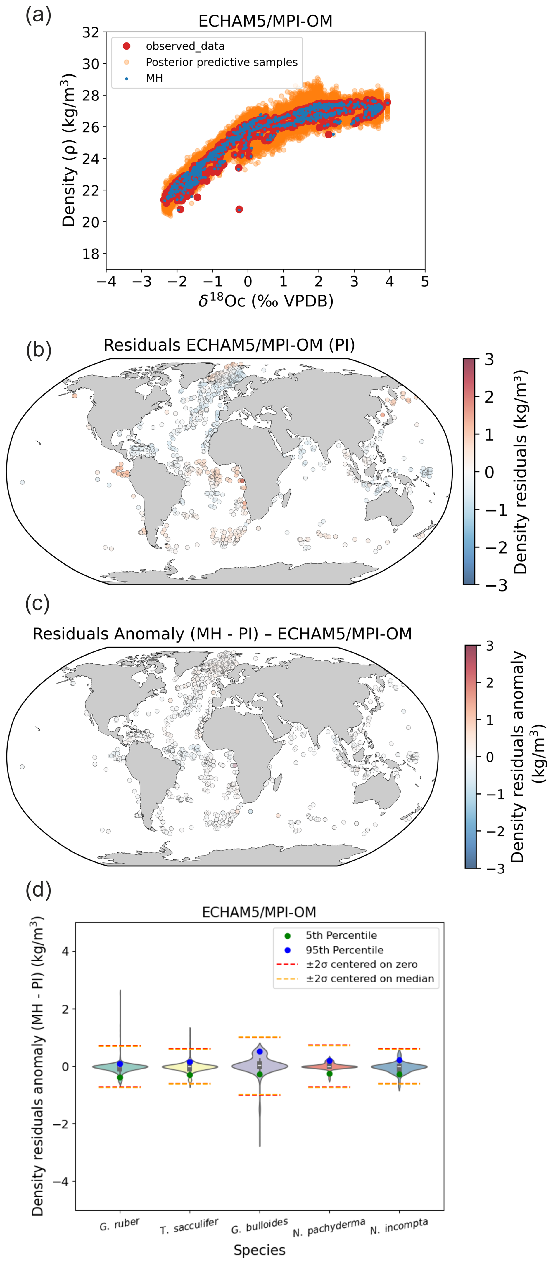
Figure B1 Stability of foraminifera δ¹⁸O_c–density relations between PI and the MH calculated with FAME and forced by global AWI-ESM-2.1-wiso (Shi et al., 2023) hydrographic data. (a) PI Bayesian regression models between foraminifera δ¹⁸O_c and annual surface density. Posterior predictive samples and the MH δ¹⁸O_c–density relation (MH) are visible. (b) Density residuals (predicted–observed) for the PI experiments. (c) Density residuals anomaly between MH and PI. (d) Probability distributions of surface density residuals anomaly (MH–PI) without Nordic Seas and northern North Atlantic (north of 40° N).

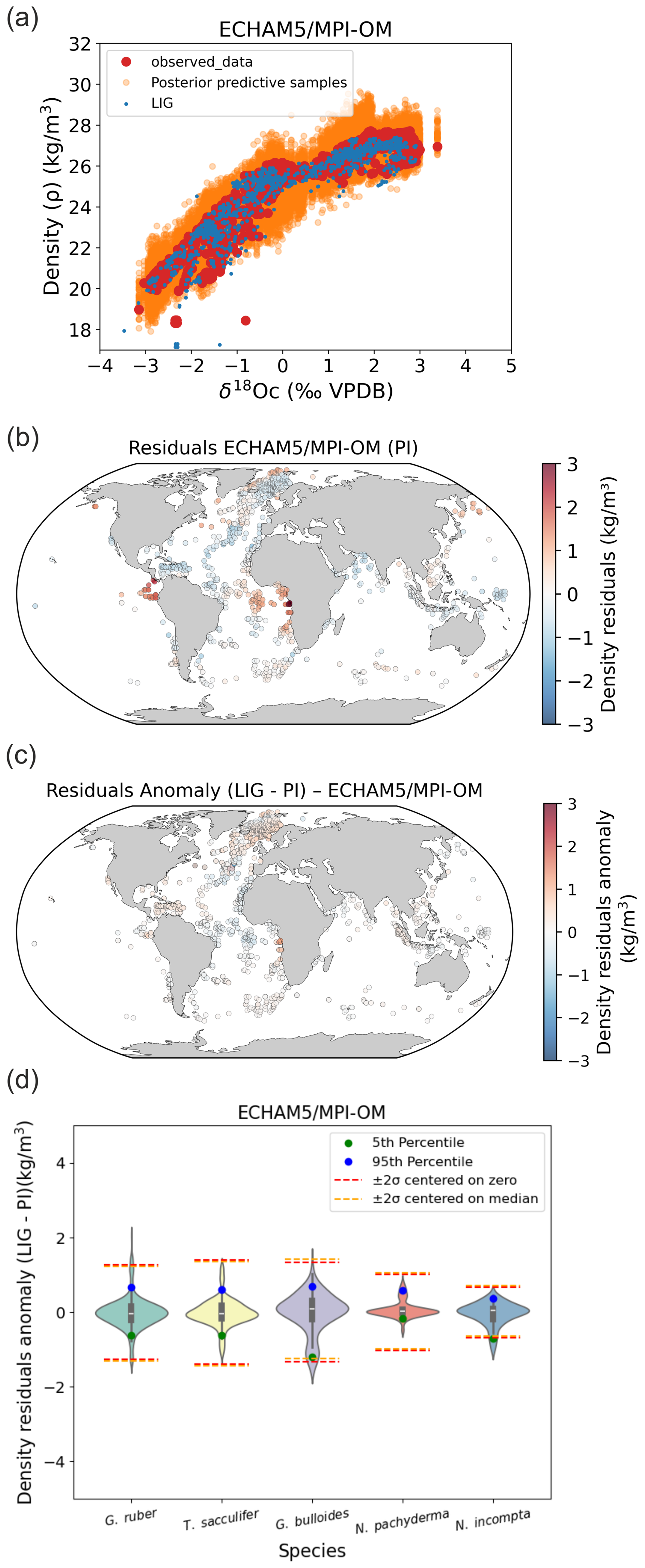
Figure B2 Stability of foraminifera δ¹⁸O_c–density relations between PI and the LIG calculated with FAME and forced by global ECHAM5/MPI-OM (Gierz et al., 2017) hydrographic data. (a) PI Bayesian regression models between foraminifera δ¹⁸O_c and annual surface density. Posterior predictive samples and LIG δ¹⁸O_c–density relations (LIG) are visible. (b) Density residuals (predicted–observed) for the PI experiments. (c) Density residuals anomaly between LIG and PI. (d) Probability distributions of surface density residuals anomaly (LIG– PI) without Nordic Seas and northern North Atlantic (north of 40° N).

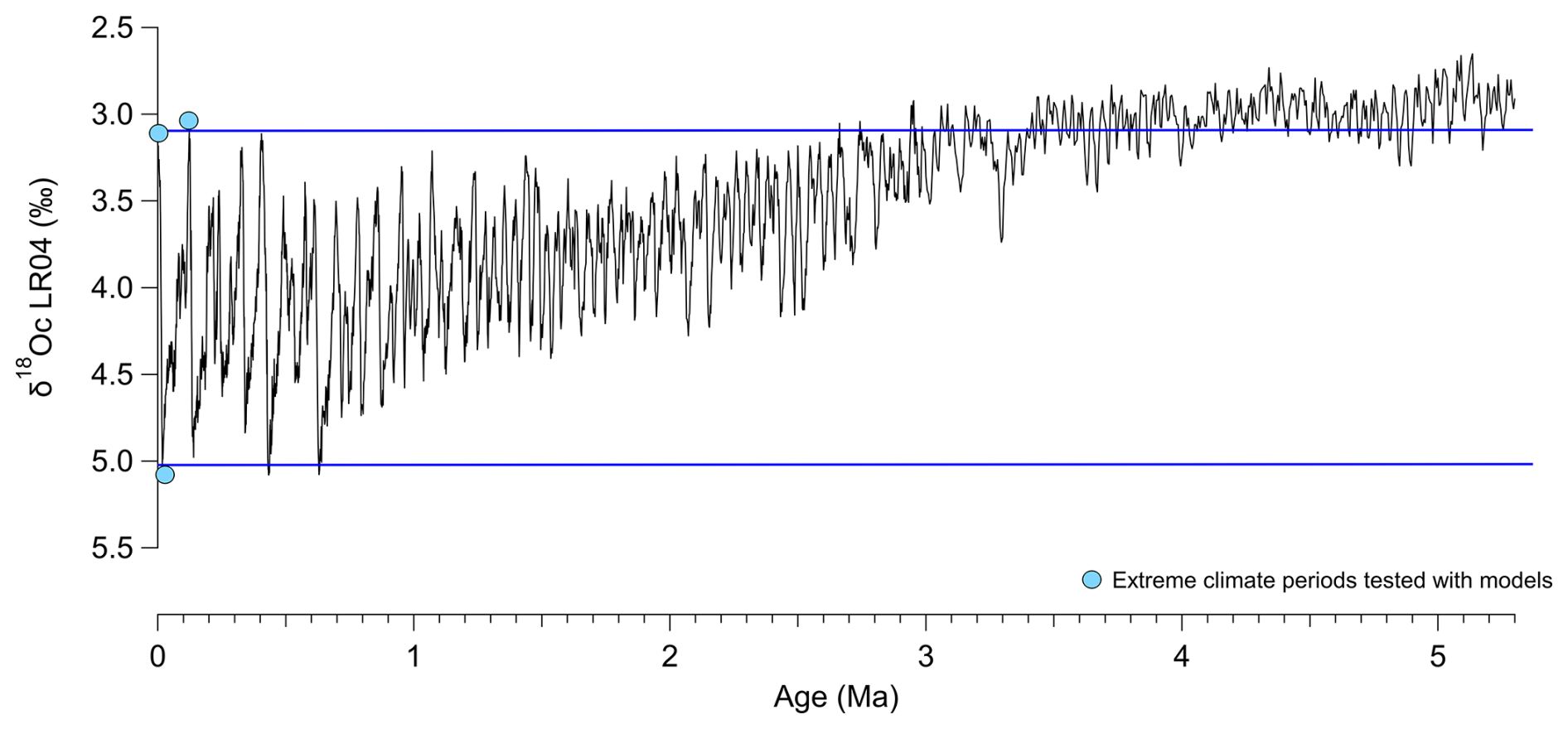
Figure B3 δ¹⁸O benthic foraminifera curve (LR04, Lisiecki and Raymo, 2005) as a proxy of ice volume and deep ocean temperature changes, used here to select extreme climatic periods (colder and more arid glacial periods versus warmer and more humid interglacial periods). Extreme climate periods tested with isotope-enabled model runs representing the mid-Holocene, LIG and LGM are represented by blue dots. Blue lines indicate the range of extreme climate conditions investigated with our climate simulations tests.

Applying our calibration to past climates (and taking into account foraminifer ecological changes) provides density predictions that remain within the uncertainties of the calibration, as demonstrated for the LGM, MH and LIG time periods. These time periods correspond to extreme climate configurations over the Quaternary period as shown on Fig. B3, so the new calibration can be reliably applied to reconstruct the past temporal evolution of ocean surface density over the entire Quaternary (last 2.6 Ma).

Nonetheless, under very extreme climates outside the Quaternary period (Fig. B3) and in ocean basins characterized by anti-estuary circulation, like the current Mediterranean Sea and Red Sea, our calibration could provide density estimates with larger uncertainty, a point that requires further investigations.