Can multi-glacier moraine analysis constrain paleoclimate reconstructions? Evidence from 3D glacier modeling in the Cordillera Real, Bolivia

Glacier moraines are widely used as proxies for past climate, as they are interpreted to reflect near-equilibrium glacier extents. However, a single glacier geometry can arise from multiple temperature-precipitation combinations and their quantification relies on glacier modeling that introduce additional uncertainties. Here, we investigate how this non-uniqueness can be constrained from a 3D full-Stokes ice-flow model (Elmer/Ice), applied to neighboring coeval glaciers in the Zongo-Charquini area of the Bolivian Cordillera Real. Using synthetic experiments, in which Temperature-Precipitation (T-P) anomaly curves are derived from several glacier extents generated under prescribed climate conditions, we show that differences in glacier geometry and hypsometry cannot be used to identify unique temperature and precipitation conditions. However, we also show that glacier thickness may provide a way to dissociate temperature and precipitation but with a limited sensitivity that would require highly accurate past volume estimates to be useful in practice, which is often not feasible. Using real moraine records, our results show that single-glacier reconstructions are strongly influenced by both, methodological choice (melt model), and site-specific uncertainties, resulting in a range of T-P anomaly curves describing the same climate. In this context, using a multi-glacier framework allows to better assess the temperature-precipitation condition and its associated uncertainties. Using this approach combined with independent tree-ring and hydrological lake-balance precipitation reconstruction in the region, we estimate temperature anomalies of −0.8 ± 0.3 °C for the Little Ice Age and −1.3 ± 0.4 °C for the Early Holocene (∼ 10 ka BP), relative to a present-day reference climate (1950–2023).

1 Introduction

Glaciers continuously grow and shrink in response to climate variations, reshaping the landscape beneath them and leaving behind characteristic features of glacial erosion and deposition (Benn and Evans, 2010). During ice advance, glaciers may bulldoze proglacial debris, deform and transport subglacial sediment, or carry supraglacial material supplied by rockfalls. These processes can lead to the accumulation of rock debris in ridge-like formations at glacier margins, forming ice-marginal moraines (Bennett and Glasser, 2009). Such moraines provide valuable information about former glacier boundaries, and their distribution in the present-day landscape is often assumed to reflect ice positions during climatically stable periods (Barr and Lovell, 2014). Consequently, ice-marginal moraines are widely used to reconstruct the extent of former glaciers and are commonly employed as proxies for paleoclimate, based on relationships between glacier geometry and climate (e.g., Benn and Ballantyne, 2005; Putnam et al., 2012; Serra et al., 2022; Kurop and Lukas, 2024; Tielidze et al., 2025).

Ice-marginal moraines can also be used to constrain past surface mass balance (SMB; the difference between mass accumulation and ablation at the glacier surface) in order to infer past climate conditions using SMB models. These models often rely on positive degree-day (PDD) approaches (e.g., Golledge et al., 2008; Putnam et al., 2013; Seguinot et al., 2016; Eis et al., 2021), on inverse modelling approaches using ice-flow models (Višnjević et al., 2018), or on more complex surface energy balance (SEB) models (e.g., Plummer and Phillips, 2003; Malone et al., 2015; Leonard et al., 2017; Quirk et al., 2018; Autin et al., 2023). Both approaches have advantages and limitations. PDD models are simple, widely used, and generally reproduce observations reasonably well; however, the same oversimplifications that make them easy to apply also limit their reliability. In contrast, SEB models offer a more complete representation of the physical processes governing melt by accounting for spatial and temporal variations in numerous meteorological parameters – such as albedo, insolation, cloudiness, wind speed, and humidity – that influence radiative and turbulent energy exchange at the glacier surface. Although SEB models are applicable to modern, well-instrumented periods (e.g., Autin et al., 2022), applying them to past climates is limited by the scarcity of both meteorological forcing data and observations needed to constrain model parameters.

A key challenge in using ice-marginal moraines as paleoclimate proxies is that a single glacier extent can result from different combinations of precipitation and temperature (see Mackintosh et al., 2017, for a review). Consequently, paleoclimate inferences based on glacier reconstructions must remain limited to qualitative comparisons of the timing and relative magnitude of glacial advance. This ambiguity is partly mitigated by the fact that glacier mass balance is typically more sensitive to temperature than to precipitation, since temperature affects both surface melt and the phase of precipitation. As a result, comparatively large changes in precipitation are needed to offset a given temperature anomaly – glaciers typically require a ∼ 40 % increase in precipitation to compensate for ∼ 1 °C of warming (Oerlemans, 2001). This asymmetry means that even substantial uncertainty in the spatial distribution of precipitation may translate into comparatively modest uncertainty in reconstructed temperature (Rowan et al., 2014); however, obtaining an independent precipitation estimate remains a major challenge.

When available, complementary precipitation or temperature proxies can help quantitatively constrain climate reconstructions (e.g., isotopic, geochemical, or biological proxies), but such records are often scarce, thereby preventing the development of systematic methods to quantify past climate from moraines. General Circulation Model (GCM) outputs can be used for similar purposes, either to constrain or to help separate the relative contributions of precipitation and temperature when independent proxy estimates are available. Nevertheless, despite significant efforts in recent years to improve the resolution and quality of climate models, paleoprecipitation estimates remain highly uncertain. This is partly because the small-scale atmospheric processes governing precipitation are too complex to be explicitly resolved at the scales relevant to mountain glaciers, and models instead rely on empirical parameterizations of variable performance. This uncertainty is further compounded by the limited availability of observational data for model initialization, assimilation, and validation, while GCM outputs still require downscaling and bias-correction procedures that introduce additional uncertainties (Ehret et al., 2012; White and Toumi, 2013).

A further approach that has proven effective for reducing the temperature-precipitation ambiguity is to combine glacier-extent and lake-balance records from the same period within a coupled glacier-lake system (e.g., Blard et al., 2009; Martin et al., 2018, 2020; Mey et al., 2020). Because glacier and lake mass balance respond differently to climatic conditions, such coupled systems yield a single combination of temperature and precipitation that simultaneously satisfies both the paleolake hydrologic balance and the reconstructed glacier extent. By integrating two independent climate-sensitive systems, this framework effectively constrains climate inversions to a near-unique solution. Here, we ask whether several coeval and neighboring glaciers – and thus, having experienced the same regional climate – can provide a comparable constraint on the climate inversion, as their contrasting geometry, aspect, hypsometry, and size may induce different T-P sensitivities.

We test this idea using 3D full-Stokes glacier modeling, which, to our knowledge, has not previously been applied to this type of moraine-based T-P inversion. Full-Stokes modeling provides a comprehensive representation of ice dynamics, thereby minimizing potential biases associated with simplified representations of glacier flow. This allows us to assess whether differences in the inferred climatic conditions arise from the contrasting characteristics of individual glaciers, rather than from limitations of the underlying dynamical model. We follow a progressive approach – from synthetic single-glacier experiments to real multi-glacier comparisons – to assess how glacier properties and model assumptions affect the T-P solution space, and whether the contrasting sensitivities of multiple glaciers can provide complementary constraints on the same climate forcing. We examine glaciers in the vicinity of Zongo Valley in the Bolivian Cordillera Real, where we investigate both synthetic (theoretical) moraines and real moraines that were previously dated to the Early Holocene (∼ 10 ka BP) and the Little Ice Age (LIA, ∼ 1600–1850 CE).

2 Materials

2.1 Study area: the Zongo-Charquini range, Bolivia

Figure 1 Satellite image of the Zongo-Charquini area (Imagery © 2026 Airbus, © 2026 Maxar Technologies; Map data © 2026 Google Earth). Colored areas indicate the extent of the four study glaciers during the Little Ice Age (red) and the Early Holocene (blue), based on previously published moraine mapping and dating studies in the region (Sect. 2.2). Present-day (2025) glacier outlines are also shown as black dashed lines. The SAMA automatic weather station (AWS; 5050 m a.s.l.) is shown as a yellow diamond within the Zongo glacier extent.

The Zongo-Charquini area is a high-altitude mountain zone in the Cordillera Real (Bolivia; 16° S, 68° W), located 25 km northeast of La Paz. It lies between the dry Altiplano plateau to the west and the wet Amazonian basin to the east, the latter being the main source of moisture for precipitation.

The study site lies within the outer tropics, a transitional zone where tropical climate dominates during the humid austral summer, while subtropical conditions prevail during the dry austral winter. Hence, mass accumulation occurs primarily during the wet summer season, whereas ablation occurs year-round and even during the austral winter when the dry air and predominant clear-sky conditions favor mass loss through sublimation (Kaser and Georges, 1999; Wagnon et al., 1999; Favier et al., 2004). Given the highly seasonal precipitation regime, glaciers act as buffers for hydrological regime at times when rainfall is low or absent. This is of high importance for urban centers such as La Paz and El Alto, where 30 %–40 % of the potable water is supplied by the glaciers of the Cordillera Real (Vergara et al., 2007; Soruco et al., 2015).

The Zongo-Charquini area has been a focus of long-term monitoring. Since 1991, the Institut de Recherche pour le Développement (IRD, France) together with the Universidad Mayor de San Andrés (UMSA, Bolivia) have conducted glaciological monitoring on the Zongo Glacier as part of the GLACIOCLIM program (https://glacioclim.osug.fr/Donnees-des-Andes, last access: 3 November 2026), producing the longest continuous mass-balance record for a glacier in the intertropical Andes (Soruco et al., 2009). A second monitoring program on Charquini South Glacier has been active since 2002 (Rabatel, 2005; Rabatel et al., 2006), providing a second mass-balance dataset used in this study.

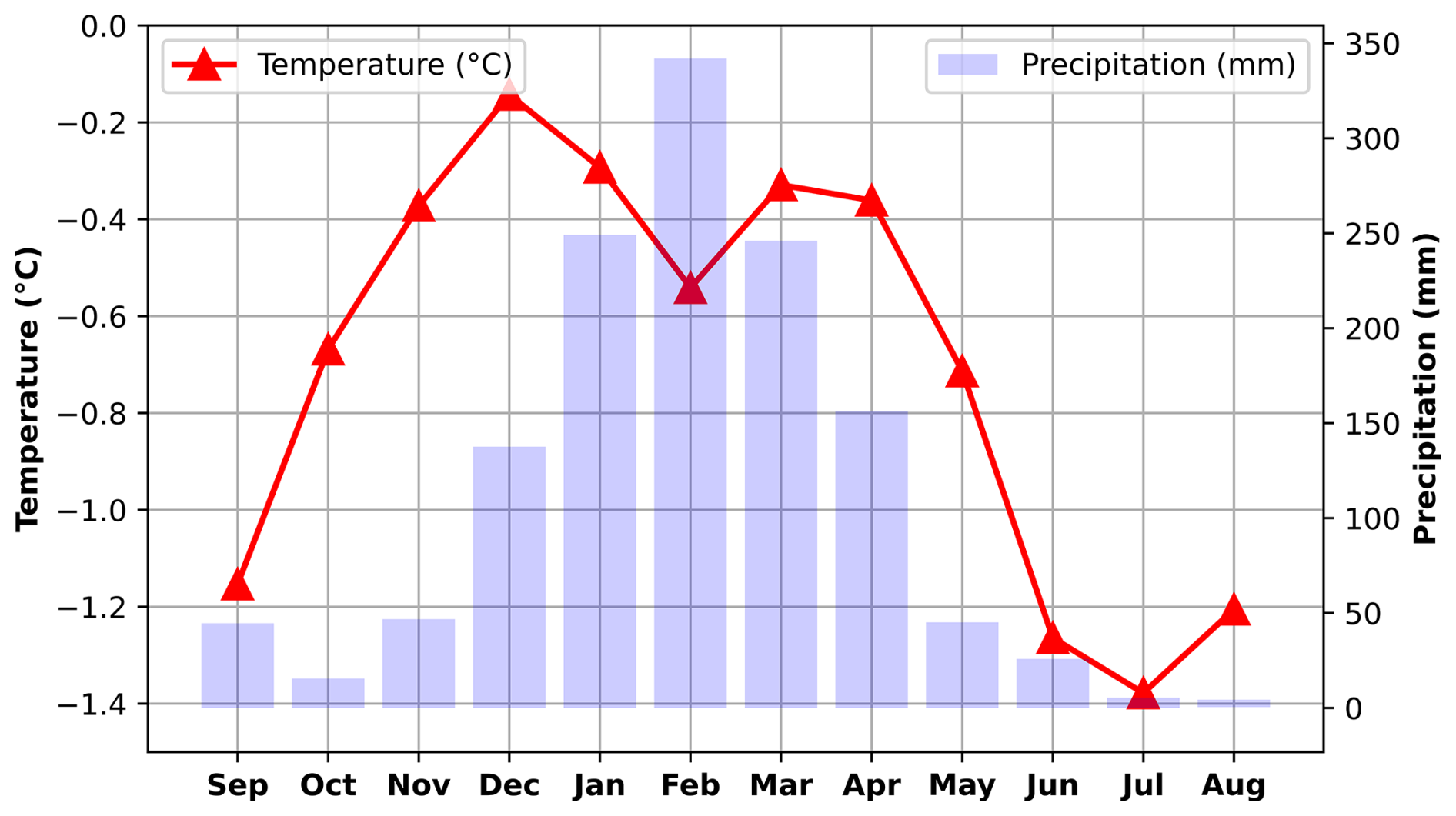
Figure 2 Typical climatic conditions in the upper reaches of the Zongo-Charquini area. The red curve shows the mean monthly temperature, and the light blue bars show the mean monthly precipitation at 5050 m a.s.l. Data are averaged over 9 non-continuous years between 1999 and 2016 and come from the SAMA automatic weather station (AWS; 5050 m a.s.l.) on Zongo Glacier (16° S, Cordillera Real), located near the present-day terminus of Zongo Glacier. Raw data are available at: https://glacioclim.osug.fr/Donnees-des-Andes (last access: 3 November 2026).

2.2 Paleoglacier marginal moraines

Most of the glaciers present today in the Cordillera Real are small ( < 0.5 km²). We interpret the observed ice-marginal moraines as recording periods when glaciers were larger than today and near mass balance equilibrium. The limited erosive effects of flowing meltwater, snowmelt, and frost penetration have preserved a well-defined set of moraines, primarily composed of granodiorite and quartzite. These lithologies favor the growth of Rhizocarpon lichens (Rabatel et al., 2005; Jomelli et al., 2007; Naveau et al., 2007), which can be used for moraine dating via lichenometry, and also provide suitable material for cosmogenic nuclide dating due to the high quartz content of the quartzites.

Rabatel et al. (2006, 2008); Jomelli et al. (2011); Martin et al. (2020) have dated moraines in the valley from the Early Holocene and Little Ice Age (LIA). The Early Holocene (∼ 10 ka BP) was characterized by increased summer insolation and warmer global conditions compared to the Late Glacial period, reflecting the transition to interglacial conditions. Glaciers generally experienced sustained retreat during this time, although Jomelli et al. (2022) report a readvance during or just prior to the Late Holocene ( < 4.2 ka). The absence of mid-Holocene moraines suggests that glaciers were smaller than during the late Holocene. Later in the Holocene, the Little Ice Age (∼ 1600–1850 CE) represents a major climatic fluctuation, marked by regional cooling that was strongest in the North Atlantic but also affected tropical mountain regions and other parts of the world.

In this study, we analyzed Early Holocene and LIA ice-marginal moraines from the Zongo, Telata, Charquini South, and Charquini North glaciers (Fig. 1). The LIA moraines in the area are characterized by several stages (referred to as M1 to M10), which are representative of the different glacier advances that occurred between 1600 and 1850 (Rabatel et al., 2005). Here, we focus on the maximum LIA extent (M1) dated to around 1680 CE, except for the Zongo glacier, where a large 350 m cliff drop likely complicates the climatic interpretation of the maximum extent. For this reason, our study also considers a slightly younger moraine for Zongo, referred to as M4, which is dated to around 1760 CE (Rabatel, 2005). This allows us to contrast glacier conditions above and below this topographic break, and to assess the potential influence of topographic controls on the LIA glacier extent. Table 1 summarizes the main glacier characteristics.

Rabatel et al. (2008)Rabatel et al. (2008)Jomelli et al. (2011)Jomelli et al. (2011)Martin et al. (2020)Rabatel et al. (2006)Jomelli et al. (2022)Rabatel et al. (2006)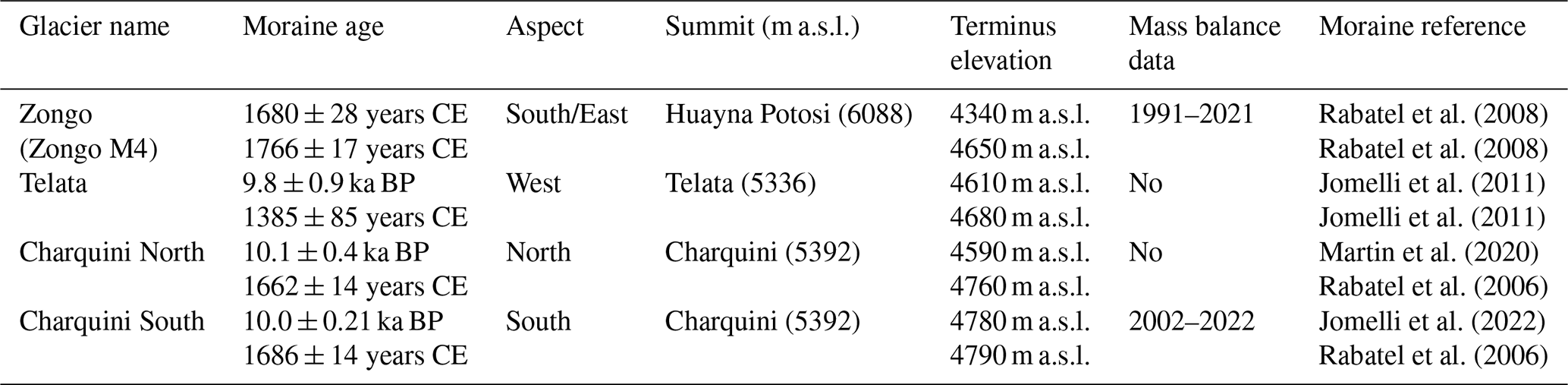

Table 1 Characteristics of the four study glaciers.

Previous studies have used the accumulation-area ratio (AAR) method or surface energy balance (SEB) modeling to estimate equilibrium-line altitudes (ELAs) for the Early Holocene and the LIA in the Zongo-Charquini area. Assuming specific precipitation conditions, these ELAs were then converted into temperature (cT) and precipitation (cP) anomalies that match the glacier extents recorded by the moraines. Table 2 summarizes the main climate reconstructions for the studied glaciers, including applied AAR values, estimated ELAs, and their respective climate anomalies.

Autin et al. (2023)Jomelli et al. (2011)Rabatel et al. (2006, 2008)Rabatel et al. (2006, 2008)Jomelli et al. (2011)Martin et al. (2020)Martin et al. (2020)

Table 2 Climate reconstructions from the Zongo-Charquini area. Temperature anomalies (cT, °C) and multiplicative precipitation factors (cP) are expressed relative to the baseline climate used in each original study. References indicate the sources of the corresponding (cT, cP) reconstructions.

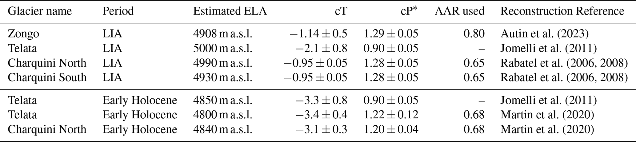
^∗cP estimated as follows: Autin et al. (2023), from on-glacier AWS record; Jomelli et al. (2011), from PMIP-II GCM ensemble; Rabatel et al. (2008), from ELA-based inversion; Martin et al. (2020), from lake–glacier inversion.

3 Methods

To investigate the evolution of the studied glaciers, we modeled glacier dynamics using Elmer/Ice (Gagliardini et al., 2013), a 3D full-Stokes numerical glacier flow model coupled with a distributed surface mass balance model. This approach is currently among the most comprehensive for simulating ice flow in mountain glacier environments, as it solves the full stress field governing ice flow without the simplifying assumptions of lower-order approximations. Accounting for the effects of climate and topography on glacier dynamics is essential to fully exploit the information recorded in ice-marginal moraines, and to accurately constrain the temperature and precipitation anomalies used in subsequent climate reconstructions.

3.1 Conceptual method

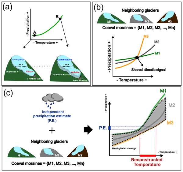
The main challenge in linking glacier extents to paleoclimate is that a single glacier extent can result from multiple combinations of temperature (T) and precipitation (P) conditions. In this study, we explore three complementary approaches to progressively reduce this range of temperature-precipitation (T-P) conditions.

We achieve this by identifying the range of (T-P) anomalies capable of reproducing a given observed paleoglacier extent. Assuming that ice-marginal moraines represent periods of climatic stability, we interpret these extents as reflecting glaciers in equilibrium with climate. By varying temperature (T) and precipitation (P) anomalies, we determine all combinations that reproduce the observed extent, defining a continuous set of T-P conditions, hereafter referred to as the T-P anomaly curve.

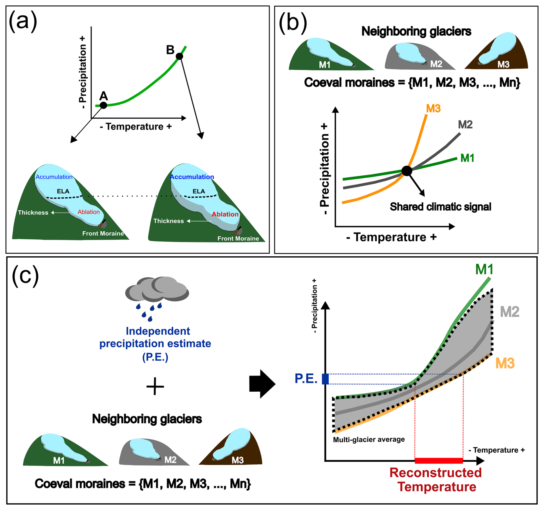
Figure 3 Conceptual framework of the methodologies: (a) Single-glacier analysis: exploring how glacier properties (e.g., ELA, volume) vary along the anomaly curve. (b) Multi-glacier method: identifying the common T-P solution from the intersection of anomaly curves from multiple neighboring and coeval glaciers. (c) Average multi-glacier method: deriving a mean T-P anomaly band across glaciers to extract the shared regional climatic signal.

Building on these curves, we then explored three approaches as follows:

• a.

  Single-glacier analysis: As a first step, we examine the characteristics of the T-P anomaly curve for an individual glacier. By analyzing how key glacier properties (e.g., ELA, volume) vary along the curve under different temperature and precipitation conditions, we assess their potential to provide additional constraints on climate. This step establishes a baseline understanding of how information from a single glacier can help restrict the range of plausible T-P combinations (Fig. 3a).

• b.

  Multi-glaciers method: Stronger constraints may be obtained by considering multiple coeval glaciers within the same area. Differences in topography and hypsometry can lead neighboring glaciers to respond differently under a common climate (Pratt-Sitaula et al., 2011). We explore this approach by jointly analyzing anomaly curves to determine the T-P conditions that satisfy all glaciers simultaneously, corresponding to the intersection of their anomaly curves (Fig. 3b).

• c.

  Average multi-glaciers method: Finally, we consider an alternative multi-glacier approach based on averaging T-P anomaly curves across several glaciers. This procedure reduces glacier-specific variability and melt model uncertainties, filtering the individual responses to emphasize the shared regional climatic signal (Fig. 3c).

Furthermore, we initially work with synthetic glacier extents moraines (see Sect. 3.4) to establish a baseline analysis, and then extend the framework to real paleoglacier moraine records. In both cases, we consider two melt models (Hock, 1999 and Oerlemans, 2001; see Sect. 3.2.2) to account for uncertainty related to the choice of mass balance formulation.

3.2 Glacier evolution model

3.2.1 Ice flow model

The ice flow is calculated by solving the Stokes equations adopting Glen's flow law with n= 3 for viscous isotropic temperate ice (Cuffey and Paterson, 2010) and is numerically solved using the Elmer/Ice finite element code (Gagliardini et al., 2013). The surface boundary condition is given by a stress-free condition, while the basal boundary condition is described by the Weertman friction law with m= 3 (Weertman, 1957) in which the friction coefficient is assumed to be spatially uniform and constant in time. The ice flow model is coupled to a surface mass balance model (see Sect. 3.2.2), so that the glacier’s upper surface evolves over time in response to both surface mass balance and ice flow (Gagliardini et al., 2013). It captures both the response of glaciers to temperature and precipitation and their interactions with bedrock topography.

For each of the four glaciers, we first defined a sufficiently wide area to fully encompass the glacier's two-dimensional horizontal footprint as indicated by the marginal moraines. Each area was meshed with triangular elements. Bedrock topography is mainly known from the present surface digital elevation models (DEMs) since the areas of interest are mainly deglaciated today (Charquini and Teleta). Bedrock topography of the Zongo Glacier is derived from radar measurements (Réveillet et al., 2015). Surface DEMs were obtained from the FABDEM v1.2 dataset (Neal and Hawker, 2023). The horizontal mesh resolution ranges from 150 m at higher elevations to 20 m near the glacier terminus (Fig. 4), allowing us to reduce computational cost while maintaining high resolution near the ice margins.

Figure 4 3D finite element mesh of Zongo Glacier. Ice flow velocity from a representative run is shown to highlight the glacier margin, front, and flow direction. The small upper-right panel shows the glacier's 2006 contour for reference. Imagery © 2026 Maxar Technologies.

Using the Benn and Hulton (2010) formulation, initial thickness fields were generated to be used as an initial condition for the glacier simulations. These initial conditions have no impact on the result as only steady state glaciers are considered in this study. The model is systematically run under constant climatic condition until reaching steady state surface topography.

3.2.2 Distributed surface mass balance model

To simulate glacier melt, we implemented the Oerlemans (2001) and Hock (1999) models, which rely on short-wave radiation and air temperature. While both models can be calibrated to reproduce present-day conditions, they differ in sensitivity away from calibration conditions, leading to potential differences in glacier response and climate reconstructions. Using both models allows us to quantify uncertainty associated with the choice of melt formulation.

The surface mass balance (SMB) is computed from daily precipitation and temperature and cumulated to obtain yearly values that are used to force the ice flow model. The local net daily SMB (m w.e. d⁻¹) is determined by A−M where A and M are respectively the local daily snow accumulation and surface melting (m w.e. d⁻¹).

The first melt model, referred to as the “Oerlemans model”, is a simplified version of the energy-balance model by Oerlemans (2001), in which short-wave radiation is estimated from potential incoming solar radiation based on surface topography only (Gilbert et al., 2023; Clauzel et al., 2023). It is expressed as:

$$\begin{array}{}\text{(1)}& M=\left\{\begin{array}{lr}\mathrm{0},& Q_{\mathrm{m}}\le \mathrm{0},\\ \frac{Q_{\mathrm{m}}\mathrm{\Delta }t}{{\mathit{\rho }}_{\mathrm{w}}{L}_{\mathrm{f}}},& Q_{\mathrm{m}}>\mathrm{0},\end{array}\right.\end{array}$$

where M is the daily melt (m w.e.), Δt the daily (= 24 × 3600 s) timestep (s), ρ_w the water density (kg m⁻³), L_f the latent heat of fusion (J kg⁻¹), and Q_m is the daily energy flux available for melt (W m⁻²), which is obtained as:

$$\begin{array}{}\text{(2)}& Q_{\mathrm{m}}=M_{\mathrm{F}}T+(\mathrm{1}-\mathit{\alpha })I+K_{\mathrm{0}}\end{array}$$

where T is the daily air temperature (°C), α the surface albedo, M_F (W m⁻² °C⁻¹) a temperature-melt factor with distinct values for ice and snow, K₀ (W m⁻²) a constant, and I (W m⁻²) is the potential incoming shortwave radiation estimated by considering latitude, slope, aspect and time of the year following Hock (1999). In this formulation, temperature and absorbed shortwave radiation contribute additively to melt energy, allowing melt to occur under subfreezing air temperatures if radiation is sufficiently strong, which is physically consistent.

The second melt model, referred to as the “Hock model”, is the temperature-radiation index model of Hock (1999), expressed as:

$$\begin{array}{}\text{(3)}& M=\left\{\begin{array}{lr}\mathrm{0},& T\le T_{\mathrm{melt}},\\ (DDF+k_{\mathrm{SW}}(\mathrm{1}-\mathit{\alpha }\left)I\right)(T-T_{\mathrm{melt}}),& T>T_{\mathrm{melt}},\end{array}\right.\end{array}$$

where M is the daily melt (m w.e.), DDF is the temperature degree-day factor under zero-radiation conditions (m w.e. °C⁻¹ d⁻¹), T_melt (°C) is the melting threshold temperature, k_SW (m w.e. °C⁻¹(W m${}^{-\mathrm{2}}{)}^{-\mathrm{1}}$) a radiation-melt factor, α the surface albedo, and I (W m⁻²) is the same incoming shortwave radiation as defined for the Oerlemans model. In this formulation, absorbed shortwave radiation and air temperature interact multiplicatively, enhancing the model’s sensitivity to temperature as a function of slope and aspect. This is a fundamental difference with the Oerlemans model where melt sensitivity to temperature is independent of short-wave radiation.

In both melt models, the local surface albedo α is estimated based on the surface state, which can be either snow, firn, or ice. Snow and firn thicknesses are updated at a daily time step to determine α (Gilbert et al., 2020, 2023). When snow is present, α is set to α_snow and then decays exponentially with time toward α_firn (Hock and Holmgren, 2005). Once the snow and firn layers disappear, α=α_ice is applied. The temperature and precipitation data provided at 5050 m a.s.l. are distributed over the glacier surface according to altitudinal lapse rates such as:

$$\begin{array}{}\text{(4)}& \begin{array}{rl}& T(z,t)=T_{\mathrm{ref}}\left(t\right)+{\mathit{\gamma }}_T(z-z_{\mathrm{ref}})\\ & P(x,y,z,t)=P_{\mathrm{ref}}\left(t\right)(\mathrm{1}+{\mathit{\gamma }}_P(z-z_{\mathrm{ref}}\left)\right)\end{array}\end{array}$$

where z is the elevation of the surface (m), T_ref(t) and P_ref(t) are air temperature (°C) and precipitation (m w.e.) at the reference elevation z_ref= 5050 m a.s.l., and γ_T (K m⁻¹) and γ_P (m⁻¹) are constant lapse-rate parameters for temperature and precipitation, respectively.

3.2.3 Surface mass balance model calibration and validation

To drive the glacier model and calibrate the SMB, we used temperature and precipitation inputs from ERA5 reanalysis (1950–2023), downscaled with the Python toolbox TopoPyScale (Filhol et al., 2023). TopoPyScale uses methods of climate downscaling at the hillslope scale introduced by Fiddes and Gruber (2014). Temperature and precipitation are interpolated horizontally and vertically from the ERA5 gridcells to the local elevation. To ensure consistency with observations, these series were bias-corrected via quantile mapping (Cannon et al., 2015) using in-situ data from the SAMA AWS at 5050 m a.s.l., available through the GLACIOCLIM network database (https://glacioclim.osug.fr/Donnees-des-Andes, last access: 3 November 2026). Following previous studies (e.g., Autin et al., 2022; Réveillet et al., 2015), we assume a vertical air temperature lapse rate of γ_T= 0.55 K 100 m along the study site. Based on observations, no vertical precipitation lapse rate was applied (γ_P= 0). A shortwave radiation correction factor of 0.72 was used to account for cloud cover effects on incoming radiation (Autin et al., 2022). The resulting downscaled and bias-corrected climate forcing is hereafter referred to as the present reference climate. The local snow accumulation A was determined from daily precipitation using a snow/rain temperature threshold of 1 °C, which lies within the commonly observed range of rain-snow transition temperatures (Jennings et al., 2018).

Both the Oerlemans and Hock melt models were calibrated separately from each other, each using observed annual SMB data from 1991–2021 for Zongo and 2002–2022 for Charquini South. For the Hock model, the melting threshold temperature T_melt (°C) was fixed at −1 °C. For both glaciers, the ice geometry was previously constrained using satellite-derived marginal contours from 2006 (Zongo) and 2016 (Charquini South), to ensure accurate glacier-wide SMB estimates during the calibration stage. For each melt model, a grid search over albedo parameters (snow, firn, ice) and sensitivity factors for temperature and radiation was performed to identify a single best-fit parameter set, common to both glaciers. For Charquini South, the simulated SMB-elevation profile shows a good agreement with observations (Table 3). In contrast, Zongo systematically exhibits excessive accumulation at high elevations and excessive ablation at low elevations. To reconcile this bias while preserving the common albedo and sensitivity parameters, an 8 % reduction in precipitation was applied for Zongo as part of the calibration trade-off, allowing a better match to both the observed SMB profile and glacier extent (Fig. 5). We note that the Oerlemans model performs better than the Hock model at simulating both glacier SMBs, as we had to use a different value of DDF for Charquini and Zongo in the Hock model (see Table 3). For validation, we used the period when the Zongo Glacier was in a relatively steady state (1956–1975; Soruco et al., 2009) to drive the model to equilibrium with our present reference climate. The resulting modeled glacier extents were then compared with the 1975 Zongo contour and the 1983 Charquini South contour derived from aerial photogrammetry (Rabatel et al., 2006; Soruco et al., 2009), demonstrating a good relationship between modeled glacier extent and climate in our model, at least for the current climate (Fig. 5). With no observation data available for the Charquini North and Telata glaciers, we applied the parameter set calibrated on the Charquini South glacier, assuming that their comparable hypsometries would result in close melt behaviors.

To account for uncertainty in model calibration, we characterized a plausible range of parameter sets around the best-fit calibration. To this end, albedo parameters were kept fixed at their best-fit values, and parameters such as the precipitation lapse rate were kept at their observationally constrained values. We instead varied the melt factors (M_F), DDF, and k_SW, as these are the parameters controlling the SMB model's sensitivity to temperature and, consequently, the climate reconstruction. For the Oerlemans model, minimum and maximum bounds were defined by varying the snow and ice melt factors (M_F,snow, M_F,ice) between 3–5 and 10–20 W m⁻² °C⁻¹, respectively, with K₀ adjusted accordingly. For the Hock model, T_melt was varied between 0 and −3 °C; since T_melt= 0 °C did not yield an acceptable fit to the observed SMB profile for either glacier, the upper bound was set at $T_{\mathrm{melt}}=-$1 °C for both, with DDF and k_SW adjusted accordingly (Table 3; Fig. A1 in the Appendix). For Charquini South, this upper-bound parameter set coincides with the best-fit calibration, as the only combination of DDF and k_SW yielding an acceptable fit at $T_{\mathrm{melt}}=-$1 °C was the best-fit combination itself. These bounds are shown as shaded uncertainty bands in the T-P anomaly curves derived from real moraines (Fig. 9).

Table 3 Calibration parameters and minimum/maximum calibration bounds for Zongo and Charquini South glaciers for the Oerlemans and Hock melt models.

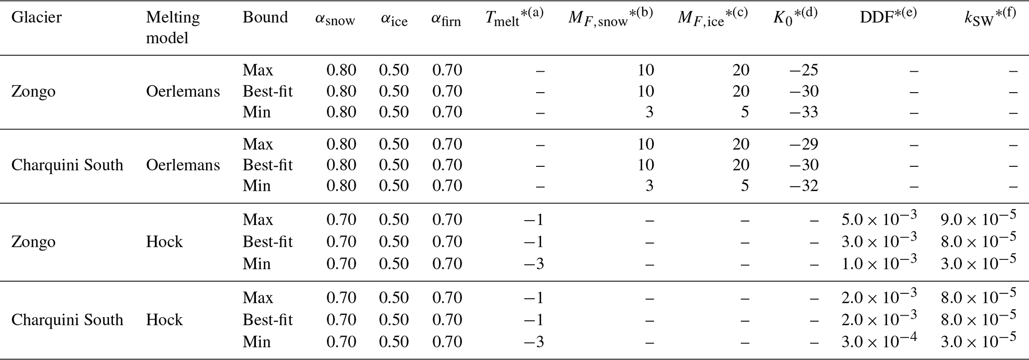
^∗Units:^(a) °C; ^(b,c) W m⁻² °C⁻¹; ^(d) W m⁻²; ^(e) m w.e. °C⁻¹ d⁻¹; ^(f) m w.e. °C⁻¹ (W m${}^{-\mathrm{2}}{)}^{-\mathrm{1}}$.

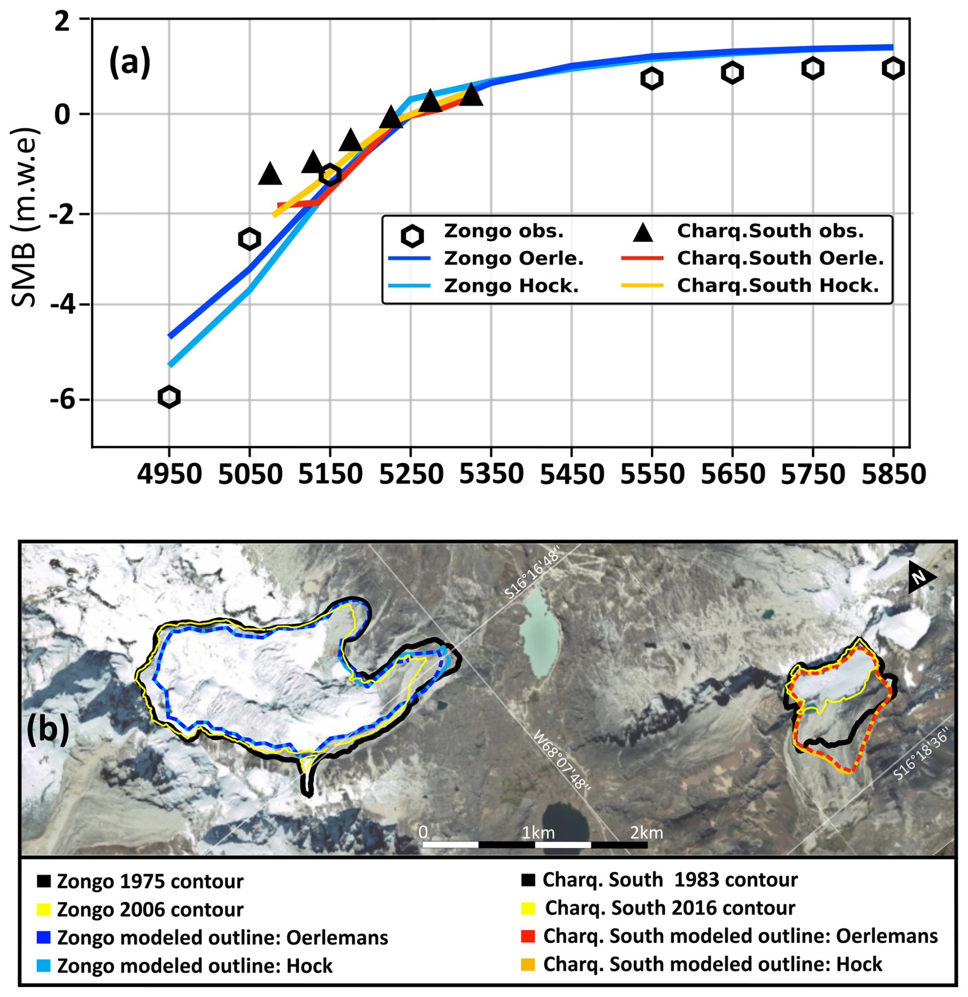
Figure 5 Results of the calibration and validation of the Oerlemans and Hock melt models using the best-fit parameter set. Panel (a) compares modeled and observed mean SMB as a function of elevation (averaged over the calibration period) for Zongo (1991–2021) and Charquini South (2002–2022). Panel (b) shows a panoramic view of both glaciers, comparing observed and modeled glacier outlines for calibration and validation. Basemap data © 2015 Google (Google Maps Satellite via QuickMapServices, QGIS).

3.3 Temperature-Precipitation anomaly curve formulation

To build the T-P anomaly curve for a given paleoglacier, temperature and precipitation from the present reference climate are perturbed by applying constant anomalies:

$$\begin{array}{}\text{(5)}& (T,P)=(T_{\text{ERA5}}+\mathrm{cT},P_{\text{ERA5}}\cdot \mathrm{cP}),\end{array}$$

where cT and cP denote constant temperature and precipitation anomalies applied to the daily time series.

For a given anomaly pair (cT,cP), the glacier SMB is computed annually over the full length of the perturbed climate time series. To represent a glacier in equilibrium with an imposed steady climate, the annual SMB values are averaged and applied as a constant forcing in the ice-flow model. This allows the glacier geometry to progressively adjust to the imposed climatic conditions until equilibrium is reached.

The glacier is considered to have reached equilibrium when its total volume changes by less than a prescribed tolerance λ> 0 over a time window Δt> 0, that is,

$$\begin{array}{}\text{(6)}& {\displaystyle \frac{\left|{\text{Volume}}^{(T,P)}(t+\mathrm{\Delta }t)-{\text{Volume}}^{(T,P)}\left(t\right)\right|}{{\text{Volume}}^{(T,P)}\left(t\right)}}\le \mathit{\lambda },\end{array}$$

where Volume^(T,P)(t) is the total glacier volume at time t under the climate conditions (T,P).

Once an equilibrium is reached, the modeled glacier front position X_mod(T,P) is compared with the observed front position defined by the marginal moraine $X_{\text{obs}}=(x_{\text{obs}},y_{\text{obs}}$). Their mismatch is quantified using the Euclidean distance:

$$\begin{array}{}\text{(7)}& d(T,P)=\left|\left|X_{\text{mod}}\right(T,P)-X_{\text{obs}}\right||.\end{array}$$

If this distance is less than a prescribed tolerance ϵ, the corresponding climate conditions are considered valid, representing plausible climate conditions at the time of moraine formation. Repeating this procedure over multiple temperature-precipitation anomaly pairs identifies a set of valid conditions that trace a curve in temperature–precipitation anomaly space. In this study, the distance tolerance is set to ϵ= 20 m, the equilibrium criterion to λ= 0.001 of glacier volume change, and the time window to Δt= 10 years.

3.4 Synthetic moraine generation

To explore the behavior of the T-P anomaly curves under controlled conditions, we constructed a set of synthetic moraines from the glacier model. All modeled glaciers evolved to equilibrium under a prescribed climate forcing (cT_syn, cP_syn)= (−1, 1), and the resulting glacier front positions were recorded as the coordinates of the corresponding synthetic moraines. These positions were then used to compute and analyze the T-P anomaly curves in this idealized scenario.

These synthetic moraines rely on a few simplifying assumptions that facilitate interpretation and provide a known set of glacier front positions, free from some of the uncertainties inherent to real moraine data. First, all synthetic moraines are coeval by construction, eliminating uncertainties related to moraine dating. Second, the resulting moraine positions are directly controlled by the imposed climate forcing, thereby removing uncertainty associated with the accuracy of the melt model.

The resulting glacier extents obtained under the prescribed climate forcing are shown in Fig. 6. Due to their differing sensitivities to temperature and incoming radiation, the Oerlemans and Hock melt formulations produce different glacier extents under identical climate conditions, with the Hock model generally yielding slightly lower glacier termini.

Figure 6 Synthetic glacier extents for the four modeled glaciers under an artificial climate anomaly (cT_syn, cP_syn) = (−1, 1). Extents were generated independently using the Oerlemans (blue) and Hock (red) mass balance models: (a) Zongo, (b) Telata, (c) Charquini North, and (d) Charquini South glacier. Basemap data © 2015 Google (Google Maps Satellite via QuickMapServices, QGIS).

4 Results

4.1 Synthetic moraines

4.1.1 Single-glacier analysis

We first analyze each synthetic glacier extent independently. While all T-P pairs along the anomaly curve reproduce the same glacier front position and equilibrium-line altitude (ELA), they yield different surface mass balance gradients and, consequently, distinct glacier thicknesses. In particular, glaciers tend to thicken under progressively warmer and wetter conditions, reflecting the increased ice flux required to maintain the same terminus position under a higher ablation regime. The magnitude of this thickness variation depends on both the melt formulation and glacier-specific characteristics. Figure 7 illustrates this relationship for the Charquini South Glacier using both the Hock and Oerlemans melt models under two temperature anomaly scenarios, together with the corresponding longitudinal and cross-sectional ice thickness profiles.

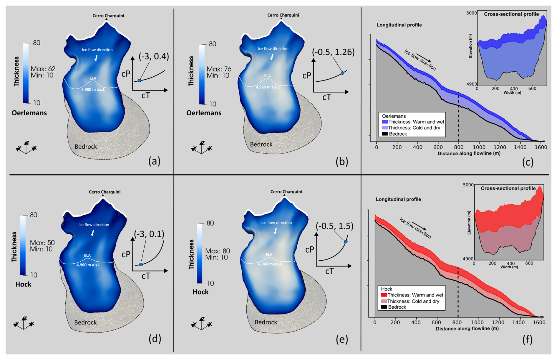
Figure 7 Charquini South Glacier thickness derived from synthetic glacier extents using the Oerlemans (blue) and Hock (red) melt models. Two climate scenarios are shown: a cold-dry case (left column, a and d; cT = −3 °C) and a warm-wet case (right column, b and e; cT = −0.5 °C). Panels (c) and (d) show longitudinal (flowline) profiles for the two melt models, while the insets show cross-sectional profiles at the locations indicated by dashed vertical lines.

4.1.2 Multi-glacier method on synthetic moraines

Figure 8 shows the T-P anomaly curves obtained for the ensemble of synthetic moraines. The Hock formulation yields systematically steeper and more convex curves than the Oerlemans model, reflecting a stronger sensitivity to temperature relative to precipitation. As imposed by the experimental design, all curves intersect at the synthetic climate (cT_syn, cP_syn)= (−1, 1).

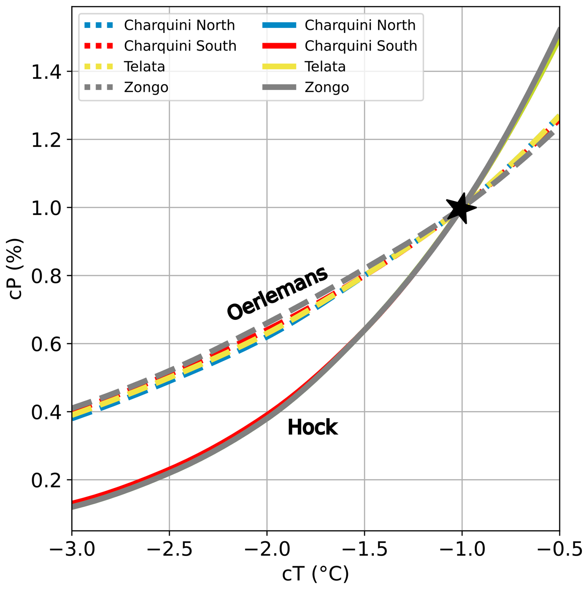
Figure 8 Synthetic T-P anomaly curves for Oerlemans (dashed lines) and Hock (solid lines) models. The black star denotes the imposed climate correction used for the synthetic moraine creation, relative to our present reference climate.

Despite differences in glacier hypsometry and aspect, the anomaly curves produced by a given melt model show near-complete overlap. The slightly larger spread of the Oerlemans curves remains within the method's inherent variability. As a result, glaciers with similar T-P sensitivities produce nearly indistinguishable curves, and their intersections do not uniquely constrain climate. In real-world settings, local variability and glacier-specific dynamics affecting moraine formation, deposition, and preservation would likely increase curve separation, as different glaciers do not record climate in exactly the same way.

4.2 Early Holocene and Little Ice Age moraines

4.2.1 Multi-glacier method on real moraines

Figure 9 presents the T-P anomaly curves derived from Early Holocene and LIA moraines, with shaded bands indicating the uncertainty range obtained from the minimum and maximum calibration bounds of each melt model (Sect.3.2.3). As in the synthetic experiments, the Hock melt model produces steeper and more curved anomaly relationships than the Oerlemans formulation, indicating that the choice of melt model strongly influences the inferred temperature-precipitation sensitivity. In contrast to the synthetic case, the real anomaly curves do not overlap but are shifted in T-P space, while remaining broadly parallel across glaciers for each melt model. For most glaciers, the curves show a consistent clustering, indicating similar T-P conditions despite small glacier-specific differences: Telata and Charquini North exhibit similar Early Holocene reconstructions, while Charquini North, Charquini South, and the inner Zongo moraine (M4) cluster closely during the LIA. In contrast, the mapped LIA maximum extent at Zongo yields a distinct T-P signal in both melt models, clearly separated from the other glaciers.

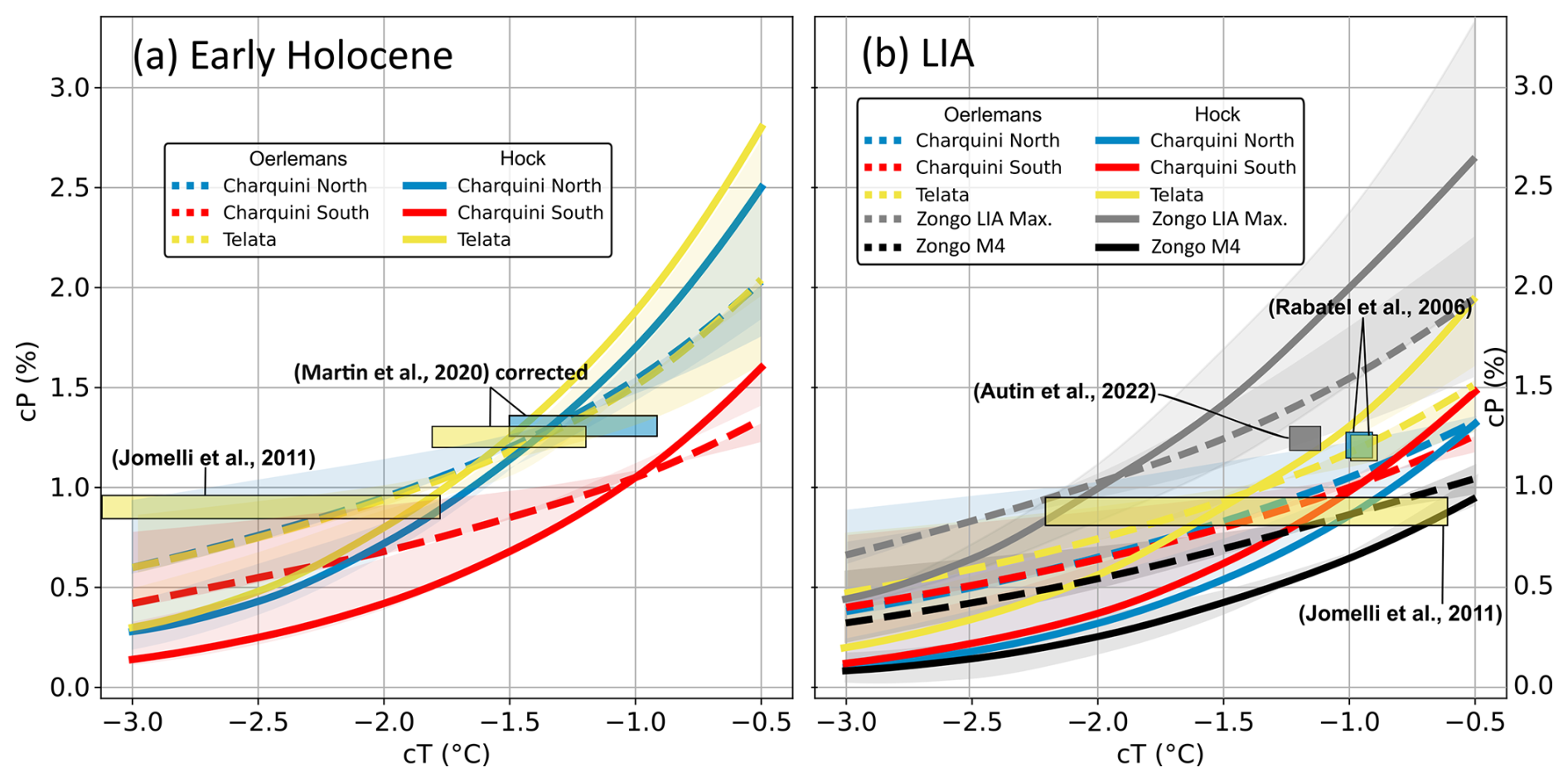
Figure 9 T-P anomaly curves for Oerlemans (dashed lines) and Hock (solid lines) models on real moraines. Moraines dated from: (a) Early Holocene, (b) LIA. Shaded bands represent the uncertainty range derived from the minimum and maximum calibration bounds of each melt model. Pale-colored rectangles depict climate reconstructions from previous studies; colors correspond to the moraine used. Temperature anomalies have been adjusted to our present reference climate for ease of comparison.

Figure 9 also includes previously published climate reconstructions for comparison. Values may differ from those reported in Table 2 because temperatures were converted to our present-day reference climate to facilitate comparison. In Martin et al. (2020), the climate reconstruction is based on precipitation estimates from Altiplano weather stations, which underestimate precipitation and lead to a cold bias in temperature anomalies. We therefore recalculated their cT-cP values using precipitation consistent with the present-day ELA at Zongo (Condom et al., 2007), which reduces this bias and yields similar cP values but ∼ 2 °C warmer cT estimates (Fig. 9a). Reconstructions from Rabatel et al. (2008); Autin et al. (2023) are also shown for the LIA.

4.2.2 Average multi-glacier method on real moraines

We applied the multi-glacier averaging approach by computing the mean T-P anomaly curve across glaciers, as shown in Fig. 10. Both the Hock and Oerlemans melt models are used to account for uncertainty associated with the choice of the mass balance formulation. Zongo is excluded from the average due to uncertainties in its mapped LIA maximum extent, which appears to be influenced by local topographic controls. To constrain the precipitation axis and derive temperature anomalies, we use independent estimates of relative precipitation changes from paleoclimate reconstructions. For the LIA, we adopt a  20 %–30 % increase relative to present conditions, based on tree-ring-based precipitation reconstructions from the Altiplano (Morales et al., 2012). For the Early Holocene, we rely on hydrological reconstructions that inverted possible climatic precipitation-temperature solutions from paleolake levels in the Altiplano (Martin et al., 2020) indicating generally wetter conditions of similar magnitude .

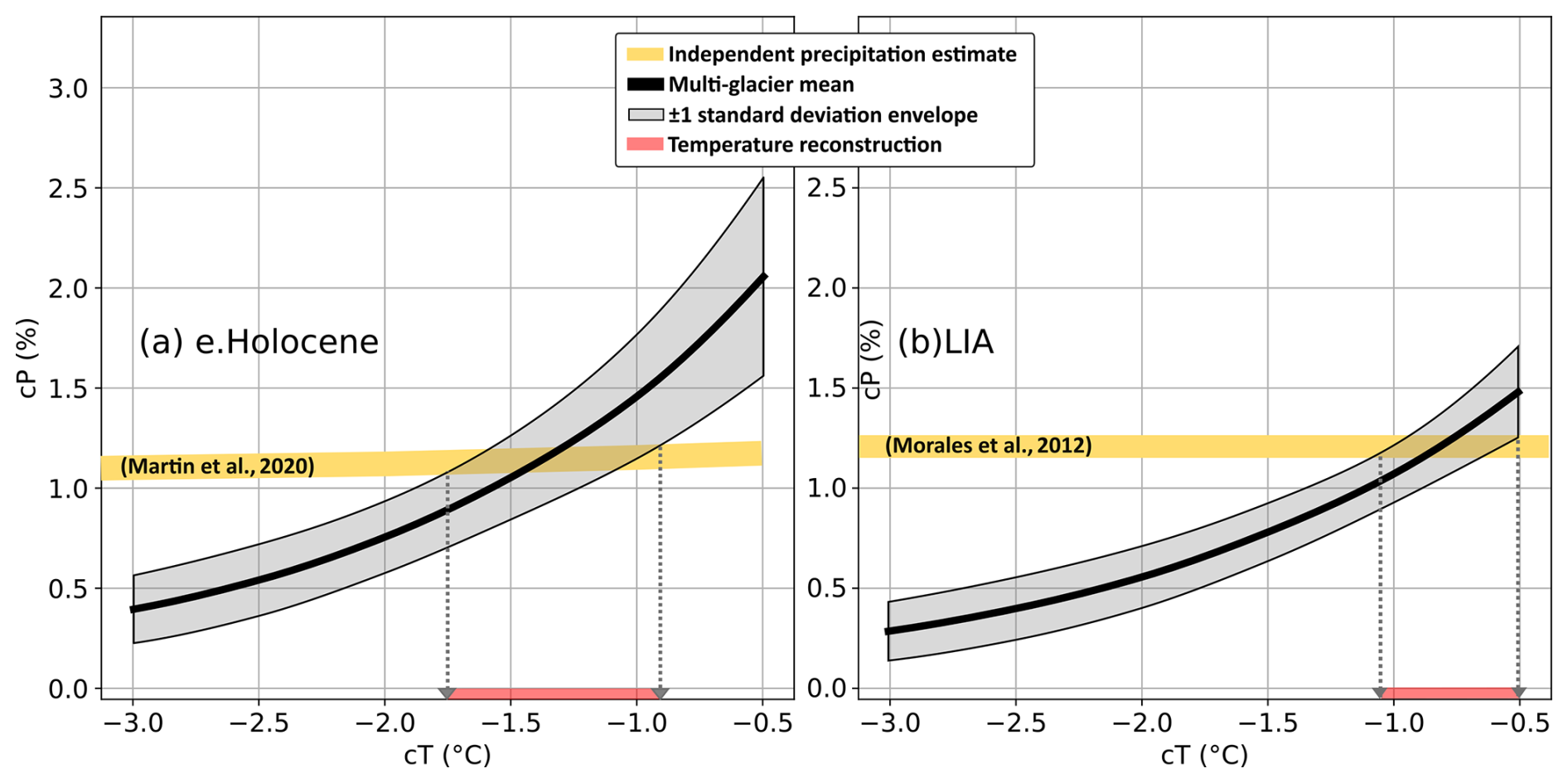
Figure 10 Multi-glacier mean T-P anomaly curves (black) for the Oerlemans and Hock models, with grey shading indicating ±1 standard deviation across glaciers. Independent relative precipitation estimates from Martin et al. (2020) (a) and Morales et al. (2012) (b) are shown in yellow; reconstructed temperature ranges are shown in red.

Based on these precipitation constraints, the multi-glacier reconstruction yields a temperature anomaly of −1.3 ± 0.4 °C relative to the present reference climate for the Early Holocene, and −0.8 ± 0.3 °C for the LIA. Additional reconstructed parameters, including equilibrium-line altitude (ELA) and accumulation-area ratio (AAR), are summarized in Table 4 for each glacier, time period, and melt model, whereas Fig. 11 shows the comparison between reconstructed ELA and AAR values from previous studies and the modeled values obtained in this study.

Table 4 Estimated ELA and AAR for each glacier under the Oerlemans and Hock melt models.

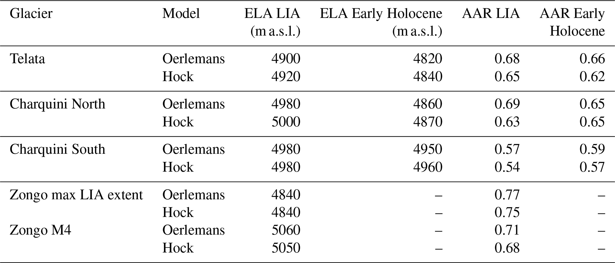
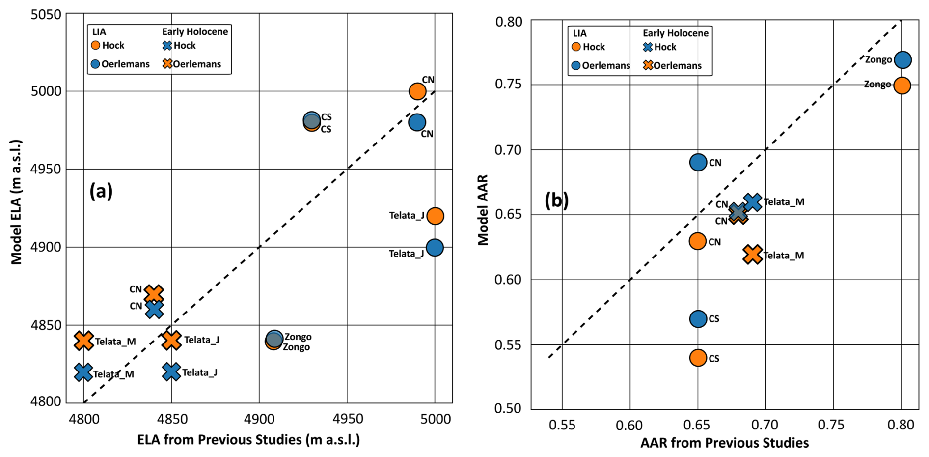
Figure 11 Comparison between glacier reconstructions from previous studies and the modeled values obtained in this study for (a) equilibrium-line altitude (ELA) and (b) accumulation-area ratio (AAR). Crosses denote the Early Holocene, whereas circles represent the Little Ice Age (LIA). Blue and orange symbols correspond to simulations performed with the Oerlemans and Hock melt models, respectively. The dashed black line indicates the 1:1 relationship between reconstructed and modeled values. Telata_J and Telata_M refer to the glacier reconstructions of Jomelli et al. (2011) and Martin et al. (2020), respectively.

5 Discussion

5.1 Can temperature and precipitation changes be dissociated from the analysis of glacier extent alone?

Our synthetic experiments show that ice thickness varies along the T-P anomaly curve, while glacier extent and ELA remain invariant (Fig. 7). These systematic variations could provide a potential additional constraint on the climate inversion problem by comparing modeled thickness along the T-P anomaly curve with independent estimates of past ice thickness. However, several caveats must be considered. First, the magnitude of these variations depends strongly on the choice of melt model, as illustrated by the longitudinal and cross-sectional profiles (Fig. 7), where the Hock model yields an increase of nearly 100 % in ice volume when transitioning from cold and dry to warm and wet conditions, whereas the Oerlemans formulation produces a more moderate increase of  32 %. Such a limited variation would imply that highly detailed geomorphic constraints, such as sharp-crested lateral moraines or trimlines, would be required to meaningfully reduce uncertainties in reconstructions that combine glacier extent and ice thickness, which are often not available in practice.

On the other hand, the choice of melt model also shows a clear impact on the T-P anomaly curves from the synthetic glacier extents, with the Hock model reflecting a stronger sensitivity to temperature relative to precipitation than Oerlemans. While the curves intersect at the imposed climatic reference state, they progressively diverge away from this point, highlighting how inferred climate conditions are highly sensitive to the choice of melt model and to departures from the calibration conditions, which by construction correspond to the imposed climate in the synthetic experiment. This also reinforces the limitation discussed above: an accurate estimate of past ice thickness would still not resolve the ambiguity, as Hock and Oerlemans would map that same thickness onto different T-P solutions.

However, curves from multiple synthetic glacier extents largely overlap within each melt model, without clear intersection points as expected in our conceptual scheme (Fig. 3b). This indicates that, within the range of geometries, differences in hypsometry and aspect alone are insufficient to generate distinct sensitivity to temperature change, meaning that temperature and precipitation solutions cannot be separated within the synthetic system. In addition, variability in accumulation related to a rain-snow threshold is not represented in our setup, as most precipitation falls as snow across the glacier elevation range, which may further reduce inter-glacier contrasts. Under these simplified, steady-state conditions, glacier extent is primarily governed by surface mass balance (SMB), largely independent of the ice flow model, which mainly acts through feedbacks between surface elevation and SMB. As a result, glaciers do not incorporate additional local or transient effects that may influence how they record climatic conditions, leading all glaciers to converge toward a common T-P solution. In real systems, however, this overlap does not necessarily hold, as transient glacier dynamics – not captured by our steady-state comparison – can decouple a glacier's response from the shared climate signal. Pratt-Sitaula et al. (2011), for instance, show that two neighbouring glaciers responded in opposite ways to the same imposed climate change, as a rise in ELA expanded the accumulation area of the higher-altitude glacier while leaving the lower one mostly below the new ELA. A synchronous response should therefore not be expected a priori when climatic conditions inferred from one glacier are applied to another, as moraines from different glaciers do not necessarily record identical climatic signals.

5.2 Variability of the reconstructed T-P curve for the studied area

In the case of real moraines, the glacier T-P anomaly curves do not overlap as for the synthetic case, but remain roughly parallel across glaciers (Fig. 9). This reflects glacier-specific sensitivities that are not fully captured by the melt model, as well as additional sources of variability such as moraine formation processes and dating uncertainties. For the Early Holocene, the Charquini South moraine indicates relatively warm conditions, comparable to mid-Holocene warmth, whereas Telata and Charquini North suggest cooler conditions, potentially closer to the Younger Dryas (∼ 12 900–11 700 BP). During the LIA, Telata records cooler conditions, while Charquini North and Charquini South cluster under similar, slightly warmer conditions, consistent with their nearly contemporaneous ages.

In the case of Zongo, and despite the age difference, the T-P curve from moraine M4 reflects conditions that align well with those of the other glaciers during the LIA. Moreover, the marked difference between moraine M4 and the mapped Zongo LIA maximum extent would imply a rapid ∼ 1.5 °C temperature shift between the Early and Late LIA, calling into question its climatic interpretation. Results from the surface energy balance analysis of Autin et al. (2023) show that uniform cooling alone cannot reproduce the Zongo maximum LIA extent without enhancing albedo effects through changes in the seasonal distribution of precipitation. In terms of equilibrium line altitude, they obtained values of 5000 and 4908 m a.s.l. for the simple cooling and precipitation-distributed scenarios, respectively. The former is consistent with our reconstructed ELA for M4 (5060 m a.s.l.), whereas the latter matches our estimate for the mapped LIA extent (4840 m a.s.l.), suggesting that simple climatic cooling is sufficient to explain M4, but not the mapped Zongo maximum LIA extent. Regional geomorphological patterns show that glaciers in the Cordillera Real preserve a consistent sequence of ∼ 10 closely spaced moraines (Rabatel et al., 2008), whereas Zongo exhibits a pronounced elevation gap between the mapped LIA maximum and the subsequent moraine sequence. This gap coincides with a steep ∼ 400 m drop at the glacier front, with moraine M4 representing the last geomorphologically stable position prior to this topographic break. We hypothesize that this drop defines a threshold beyond which topography strongly modulates ice dynamics, allowing the glacier to extend to lower elevations. During the LIA maximum, a serac fall likely split the Zongo Glacier in two at this location. Assuming continuous ice flow thus introduces a bias in climate reconstruction that likely explains the anomalous climatic signal associated with the mapped extent of the Zongo LIA maximum.

5.3 Multi-glacier averaging for robust climate reconstruction

So far, our results highlight the strong influence of melt model choice on the reconstructed climatic signal, and show that glacier responses are not solely governed by hypsometry and aspect – which, as discussed in Sect. 5.1, are insufficient alone to constrain the T-P solution – but also modulated by further glacier-specific factors that introduce additional uncertainty into single-glacier climate reconstructions. Consequently, climate reconstruction based on a unique glacier should be approached with caution. For this reason, we rely on a multi-glacier averaging approach as the basis for our climate reconstruction, as combining multiple glaciers and melt models reduces the influence of site-specific effects and provides a more robust estimate of regional climatic conditions. Still, this approach remains sensitive to extreme values and can be biased by glaciers that deviate strongly from the regional signal, underscoring the importance of a careful climatic and geomorphological interpretation of the moraine record used. In our case, this interpretation led us to identify Zongo's mapped LIA extent as incompatible with our modelling approach, given the strong topographic modulation of ice dynamics at the glacier front and the possibility that the downstream moraines were partly fed by avalanching ice, a process not represented in our model. We therefore excluded it from the multi-glacier average. Had this incompatibility gone unnoticed, our LIA reconstruction would have been biased toward a colder estimate by 0.42 °C (Fig. A2 in the Appendix).

Our climate reconstruction indicates an Early Holocene cooling of −1.3 ± 0.4 °C, in good agreement with the revised estimates from Martin et al. (2020) (cT$=-$1.5 to −1.3 °C), yet warmer than the reconstruction based on the Telata glacier from Jomelli et al. (2011), likely due to methodological factors in that approach, including assumptions of reduced precipitation, potential overestimation of melt reflected in higher ELA, and the reliance on a single glacier. For the LIA, our reconstruction yields a cooling of −0.8 ± 0.3 °C relative to the present reference climate, in close agreement with the −0.95 °C estimate of Rabatel et al. (2006, 2008). The  0.5 °C Early Holocene-LIA difference in our reconstruction is also consistent with the pattern shown by tropical-scale model-data comparisons (Liu et al., 2014). At a broader temporal and spatial scale, this result can be compared to the global synthesis of Neukom et al. (2019), which documents coherent multidecadal temperature variability across reconstructions and model simulations. That study reports a LIA cooling of about 0.4 °C relative to 1961–1990, closely matching our estimate of approximately −0.5 °C over the same reference period. Overall, this consistency across spatial scales further supports the robustness of the regional climatic signal derived from our multi-glacier averaging approach.

5.4 Implications of the full-Stokes ice flow model

The reconstructed ELAs and AARs from our model show variable agreement with previous glacier reconstructions (Table 4; Fig. 11). In particular, Early Holocene ELA estimates tend to be more consistent across studies, whereas LIA estimates exhibit a larger spread across glaciers and reconstructions. For AAR, previous studies often adopt relatively uniform values across glaciers, whereas AAR derived from our simulations shows a wider range of glacier-specific values that more directly reflect differences in glacier hypsometry. This is particularly evident for Chaquini South, where our lower reconstructed AAR likely results from a more accurate representation of the glacier geometry, characterized by a broader and less steep accumulation area. At the same time, the reconstructed climate anomalies remain broadly consistent with independent regional estimates, supporting the robustness of our reconstruction.

Nevertheless, and despite using the most comprehensive ice-flow approximation available, we did not obtain better climate constraints than previous studies based on simpler glacier models – a comparison that, to our knowledge, had not previously been made directly for this type of reconstruction – suggesting that ice-flow complexity is not the limiting factor in this type of T-P reconstruction. Although it remains unclear how a simpler ice-flow model coupled to the same SMB formulation would perform, we would not expect an improvement in the climate constraint. This limited sensitivity of the results to the ice-flow formulation is likely because topography strongly guides and confines ice flow in mountain glacier settings, so, under steady-state conditions, glacier geometry is primarily controlled by the mass-balance distribution rather than by the specific ice-flow approximation (Oerlemans, 2001; Le Meur et al., 2004). Differences between ice-flow models become more relevant in transient simulations, where ice thickness and internal deformation actively shape the evolution of glacier geometry, and where a full-Stokes approach would therefore be expected to offer a more accurate representation of the glacier response.

5.5 Broader applicability and limitations

From a theoretical point of view, the multi-glacier full-Stokes framework presented here is transferable to other glaciated regions, subject to a few practical and conceptual considerations. First, its application requires a set of coeval, neighboring glaciers with well-preserved moraine records. The appropriate spatial and temporal configuration likely depends on the characteristics of the study area and the climatic signal being reconstructed. Therefore, testing different glacier separations and degrees of temporal overlap would help assess how these factors affect the reliability of the approach. Nevertheless, the approach may remain useful even when the available glaciers are fewer or more widely spaced, particularly in regions where other paleoclimate constraints are limited. Second, the approach relies on the availability of present-day observational data for at least one glacier in the study area, without which melt model parameters cannot be independently constrained.

Besides, the T-P constraint provided by our approach likely depends on the climatic and glaciological setting of the study area. The glaciers studied here differ in hypsometry and aspect, yet present a similarly snow-dominated precipitation regime and are similarly confined by steep valley topography. The extent to which these other features influence T-P sensitivity, and whether stronger contrasts between glaciers could provide more complementary constraints on the reconstruction, remains unclear. It would therefore be valuable to test our approach in settings where glaciers differ more strongly from each other in these respects.

A further limitation inherent to our approach, and to most glacier-based paleoclimate reconstructions, is the assumption that a mapped moraine reflects a glacier in equilibrium with a sustained climate state. However, glacier length can fluctuate substantially in response to interannual climate variability alone, even under an otherwise stationary long-term climate (Oerlemans, 2000; Roe and O’Neal, 2009; Roe, 2011; Doughty et al., 2017). Such fluctuations could, in principle, produce a moraine at a given position without reflecting a genuine, sustained shift in temperature or precipitation. In this context, the multi-glacier approach limits the effect of glacier-specific stochastic excursions on the reconstructed climate, while the agreement between the resulting T-P curves can help identify potential deviations from the common climatic signal: closely grouped curves support a common climatic interpretation, whereas a strongly deviating curve may point to glacier-specific processes or a stochastic excursion. However, this approach does not fully resolve this source of uncertainty, which remains an open challenge for the field.

6 Conclusions

We investigated how glacier-based climate reconstructions can be constrained using temperature-precipitation (T-P) anomaly curves derived from a 3D full-Stokes ice-flow model, applied to neighboring, coeval glaciers within the upper reaches of the Zongo-Charquini area in the Bolivian Cordillera Real. The analysis progresses from single-glacier synthetic experiments to real multi-glacier cases under two melt model formulations.

Our results confirm that single-glacier reconstructions remain fundamentally non-unique, as multiple combinations of temperature and precipitation can reproduce the same equilibrium state, a limitation inherent to steady-state approaches that do not account for hysteresis effects. While ice thickness could in principle provide an additional constraint on the T-P solution space, its limited variation along the T-P curve means that it would only be useful with highly detailed geomorphological constraints. Yet, even with such constraints available, the resulting T-P solution would remain melt-model dependent, as different melt models can map the same ice thickness onto different climate solutions, meaning that ice thickness alone cannot resolve the non-uniqueness of single-glacier reconstructions.

A key result is that the choice of melt model exerts a strong control on the shape of T-P anomaly curves, leading to substantial differences in inferred climate conditions, particularly away from calibration states. This highlights the sensitivity of glacier-based reconstructions to model formulation. In this context, full-Stokes modelling does not show a significant advantage over simpler approaches for glacier-extent-based reconstructions. Beyond model-related effects, real moraine systems are also influenced by glacier-specific and non-climatic factors. The Zongo case illustrates an example of how topographic constraints can bias climatic interpretations when glaciers are considered in isolation.

Taken together, these results indicate that individual glacier reconstructions are highly sensitive to model assumptions and local variability that cannot be fully constrained in practice. In this context, multi-glacier approaches provide a robust framework for estimating regional climate (e.g., Golledge et al., 2012). This robustness is supported by the consistency between our reconstructed regional climate anomalies (−0.8 ± 0.3 °C for the LIA and −1.3 ± 0.4 °C for the Early Holocene) and previous independent estimates based on different methodologies in the region. Further progress in glacier-based paleoclimate reconstructions will depend on improving our understanding of moraine formation processes and their representativeness of average climate conditions. This remains a key limitation in interpreting these landforms as quantitative paleoclimate archives and in fully exploiting their potential.

Appendix A: Supplementary figures

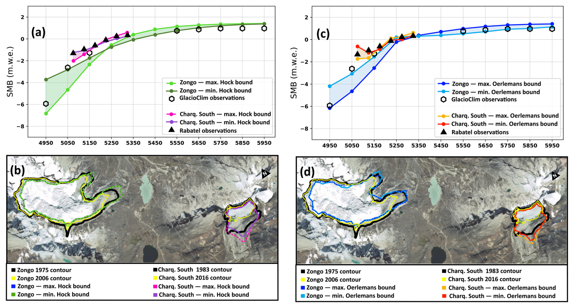
Figure A1 Minimum and maximum calibration bounds for the Hock (a, b) and Oerlemans (c, d) melt formulations, showing modeled vs. observed SMB profiles (a, c) and glacier outlines (b, d). Basemap data © 2015 Google (Google Maps Satellite via QuickMapServices, QGIS).

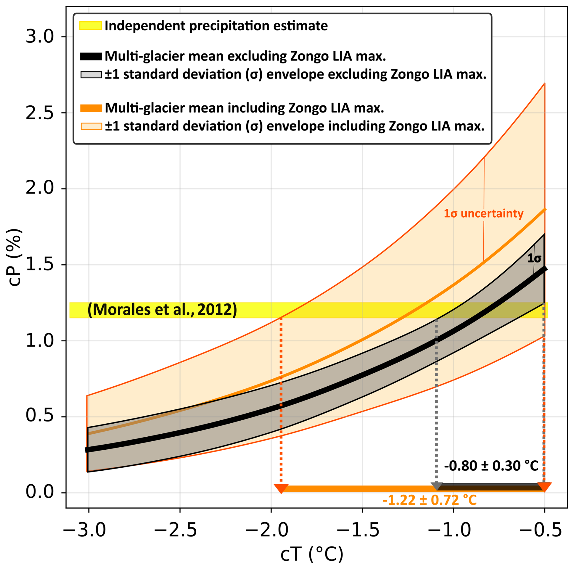
Figure A2 Sensitivity of the multi-glacier average to the inclusion of the Zongo LIA maximum extent in the climate reconstruction.