Using ocean surface paleo-density to evaluate PMIP3 and PMIP4 Last Glacial Maximum climate simulations

Quantitative reconstruction of ocean surface density during the Last Glacial Maximum (LGM) offers valuable insights into the ability of climate models to simulate past climate conditions, when global temperatures were about 4.5 to 6°C colder than today. We assess the performance of the LGM climate simulations, as part of the 3rd and 4th phase of the Paleoclimate Modeling Intercomparisons Project, using a recent ocean surface density reconstruction based on the δ¹⁸O of foraminiferal calcite (δ¹⁸O_c). We consider the differences between the LGM and the preindustrial climates and each period separately, at both global and regional scales. Because surface density reflects the combined effects of temperature and salinity, we also examined sea surface temperature (SST) to better identify the processes underlying model–data differences.

On a global scale, surface density reconstructions generally exhibit greater spatial variability than simulated surface density anomalies (LGM − PI), although part of this difference is reduced when reconstruction uncertainties are taken into account. Model simulations tend to underestimate the magnitude of reconstructed density anomalies and substantial differences between cumulative distribution persist. Part of the mismatch may arise from the uneven spatial distribution of reconstructions, which are mostly located near coastal areas.

Density anomaly (LGM − PI) differences between data and models are largely controlled by sea surface salinity (SSS), with SST contributing to a lesser extent. This influence of SSS is directly linked to the reduction in tropical precipitation during the LGM: model simulations that best match the large-scale density anomalies also simulate the strongest reductions in reconstructed low-latitude precipitation during the LGM, highlighting the key role of hydrological cycle changes in shaping surface density.

All simulations capture key features of the reconstructed surface densities when the LGM and PI periods are analysed separately at the global scale, with Taylor diagrams and complementary performance metrics indicating moderate to good overall agreement despite differences among simulations.

Regional analyses show that most simulations reproduce reconstructed Indian Ocean surface density reasonably well, although model simulations performance is systematically lower in the North Indian Ocean than in the South Indian Ocean. Focusing on the Indo-Pacific Warm Pool, proxy reconstructions indicate a weakened West-East tropical Indian surface density gradient during the LGM, but only 7 out of 14 model simulations (50 %) reproduce this feature.

These results highlight the need to improve and better constrain regional hydrological cycle changes in models, as improving their representation is crucial to reduce uncertainties in both paleoclimate simulations and future climate projections.

1 Introduction

Past surface seawater density is a key property for studying ocean dynamics, as it reflects the combined influence of surface temperature and salinity and is directly linked to circulation changes through geostrophic balance. In this study, we focus specifically on seawater surface density, providing a novel perspective in model–data comparisons for the Last Glacial Maximum (LGM), a variable that has not been explored in previous assessments.

To simulate future climate change, scientists rely on coupled general circulation models (GCMs). However, these models differ in their representation of Sea Surface Temperature (SST), Sea Surface Salinity (SSS), as well as in the processes that control density. Differences in changes of SST and SSS in the future is therefore leading to large uncertainties in the simulation of future ocean dynamics (Flato et al., 2014 – IPCC AR5; Eyring et al., 2021 – IPCC AR6).

Since climate models are developed based on present-day conditions and used to project future climates that may be very different from the present one, it is important to also evaluate them with reconstructed very different climate conditions from the past, to gain confidence in their projections. One way to test the response of these models to various external forcings is to use paleoclimate simulations, which provide an independent evaluation of model performance (Harrison et al., 2014; Kageyama et al., 2024) against available reconstructions. This allows us to benchmark models using evidence from past climates, which is essential for strengthening confidence in their future projections. The Paleoclimate Model Intercomparison Project (PMIP; Joussaume and Taylor, 1995; Kageyama et al., 2018) tests the ability of models to simulate paleoclimate reconstructions. Currently in its fourth phase (PMIP4), with a fifth in preparation, PMIP plays a critical role in evaluating how well models reproduce past climates.

One of the PMIP reference periods is the Last Glacial Maximum, which occurred between 19 000 and 23 000 years ago, when the ice sheets reached their maximum global volume (Mix et al., 2001). During this period, the climate was markedly different from pre-industrial conditions, with significantly colder temperatures (from −4.5 ± 0.9 °C according to Annan et al., 2022 to −6.1 ± 0.4 °C according to Tierney et al., 2020) and altered hydrological cycles, making it an interesting benchmark period for evaluating climate models (MARGO project, 2009; Braconnot et al., 2012).

Evaluating numerical climate models using a data-model comparison allows us to assess their robustness in simulating key variables such as sea surface temperature (SST) and precipitation (Brierley et al., 2020). Recent intercomparison studies focusing on SST reconstructions at the LGM (Tierney et al., 2020; Kageyama et al., 2021) show that models generally capture large-scale cooling patterns but still often exhibit regional biases and differences between PMIP3 and PMIP4 simulations.

To enable quantitative evaluation of ocean surface density, a new method has been developed to reconstruct annual seawater surface densities in the past (Caley et al., 2026), providing a novel tool for model assessment. However, until now, quantitative evaluations of surface density remain unexplored, which limits our understanding of how well models capture the combined effects of temperature and salinity on ocean circulation.

In this study, we make use of this new surface density reconstruction to evaluate PMIP3 and PMIP4 simulations in terms of annual ocean surface density, both on a global scale (excluding the Nordic Seas region, Caley et al., 2026) and regionally. We consider simulations of the Last Glacial Maximum (LGM) and the pre-industrial period (piControl). We focus on evaluating model performance in simulating surface density, and where there are large discrepancies between models and past reconstructions, we further investigate SST and, in combination with density, qualitative changes in SSS. This approach provides a complementary perspective to previous studies, offering new insights into the coupled role of temperature and salinity in shaping ocean surface density and allowing for a more integrated evaluation of model performance.

Our analysis is structured as follows: we first assess model simulations against past reconstructions at the global scale in Sect. 3. We then examine regional differences in Sect. 4, identifying areas where model simulations perform better or worse, with a particular focus on the Indian Ocean as a case study of regional variability.

2 Material and methods

2.1 Climate reconstructions

2.1.1 Surface ocean density

To evaluate model simulations on ocean surface density, we use the quantitative past density reconstruction dataset proposed by Caley et al. (2026). They developed a new Bayesian calibration model to calculate the annual surface ocean density using the δ¹⁸O_c (for δ¹⁸O carbonate) measurements of several foraminiferal species. Briefly, this probabilistic approach explicitly accounts for inter-species differences and calibration uncertainties, allowing quantitative density reconstructions. New and published δ¹⁸O_c datasets were compiled to create an extended database of 474 density reconstructions distributed across all oceanic regions. For each marine sediment core, reconstructions are available for both the LGM and the Late Holocene (LH) (Caley et al., 2026). The Bayesian hierarchical regression model calibrated to annual surface density yields prediction uncertainties (σ) that vary across species, ranging from 0.48 kg m⁻³ (N. pachyderma sinistral) to 0.86 kg m⁻³ (G. bulloides). More specifically, the mean calibration uncertainties are 0.74 kg m⁻³ for G. ruber, 0.73 kg m⁻³ for T. sacculifer, 0.86 kg m⁻³ for G. bulloides, 0.58 kg m⁻³ for N. pachyderma dextral, and 0.48 kg m⁻³ for N. pachyderma sinistral. When the Bayesian regression model is applied to LGM and LH δ¹⁸O_c foraminifera databases to reconstruct annual surface density during these periods, we observe stronger increase in LGM surface density value changes at low latitudes compared to mid latitudes. Analyses from the northern region > 40° N of the Atlantic Ocean were rejected due to potential errors when applying the calibration to the LGM time period (Caley et al., 2026). We thus also exclude this region for the model-data comparison. Surface density is expressed in kg m⁻³. Throughout this work, values are expressed as anomalies relative to 1000 kg m⁻³.

Concerning the instrumental observations, we used the version 4.2.2 (analyses.g10, downloaded in 2024) of the EN dataset from the Met Office Hadley Centre (Good et al., 2013), commonly referred to as EN4. This dataset provides quality-controlled ocean temperature and salinity profiles globally, as well as monthly gridded fields derived from objective analyses, covering the period from 1900 to 2022. EN4 is a compilation of temperature and, when available, salinity measurements from various ocean data sources. Surface seawater density, which is a non-linear function of temperature and salinity, was calculated from EN4 temperature and salinity fields using the GSW (Gibbs Seawater) formulation implemented in the gsw Python package (Roquet et al., 2015).

2.1.2 Sea surface temperature

Since sea surface density and SST are linked, we also performed a data/model comparison in terms of surface temperature. This provides an additional way to investigate the drivers of surface density changes. To do this, we used two previously published SST databases (MARGO Project, 2009; Tierney et al., 2020). These two databases were not combined, as the Tierney dataset includes some MARGO data but with more recent calibrations. Notably, Tierney et al. (2020) also recalibrated all age models using the Marine13 radiocarbon calibration curve and the BACON age modelling software, ensuring a better chronological consistency across records. The temporal periods differ slightly: Tierney's data refer to the LGM and the Late Holocene (LH), while the MARGO data include LGM and “pre-industrial” measurements from the WOA1998 dataset (NODC, Silver Springs, 1998). Following Tierney et al. (2020), we make here the approximation that the Late Holocene is considered representative of the pre-industrial climate state.

The MARGO database (MARGO Project, 2009) contains 821 SST reconstructions based on a diverse range of proxies, including $\mathrm{Mg}/\mathrm{Ca}$ ratios, $U_{k\mathrm{37}}^{\prime }$ indices, radiolarians, diatoms, foraminiferal transfer functions, and the tetraether index TEX₈₆. In contrast, Tierney's dataset (Tierney et al., 2020) comprises 244 SST records derived exclusively from $\mathrm{Mg}/\mathrm{Ca}$, TEX₈₆, and $U_{k\mathrm{37}}^{\prime }$ proxies. We do not use the assimilated SST product developed by Tierney et al. (2020), but only the raw SST proxy database published in association with their study. This selection reflects a deliberate choice by Tierney et al. (2020) to exclude assemblage-based proxies such as foraminiferal transfer functions, due to concerns over “no-analogue” assemblages and the lack of Bayesian calibration models, which are central to their probabilistic framework. SST values inferred from δ¹⁸O_c were also excluded from our analysis, as they were already incorporated into our density reconstructions. Finally, both SST and density datasets were re-gridded onto a common 1° × 1° spatial grid, matching the reference grid to which the model simulations were also re-gridded, allowing for a direct comparison.

2.2 Climate model simulations

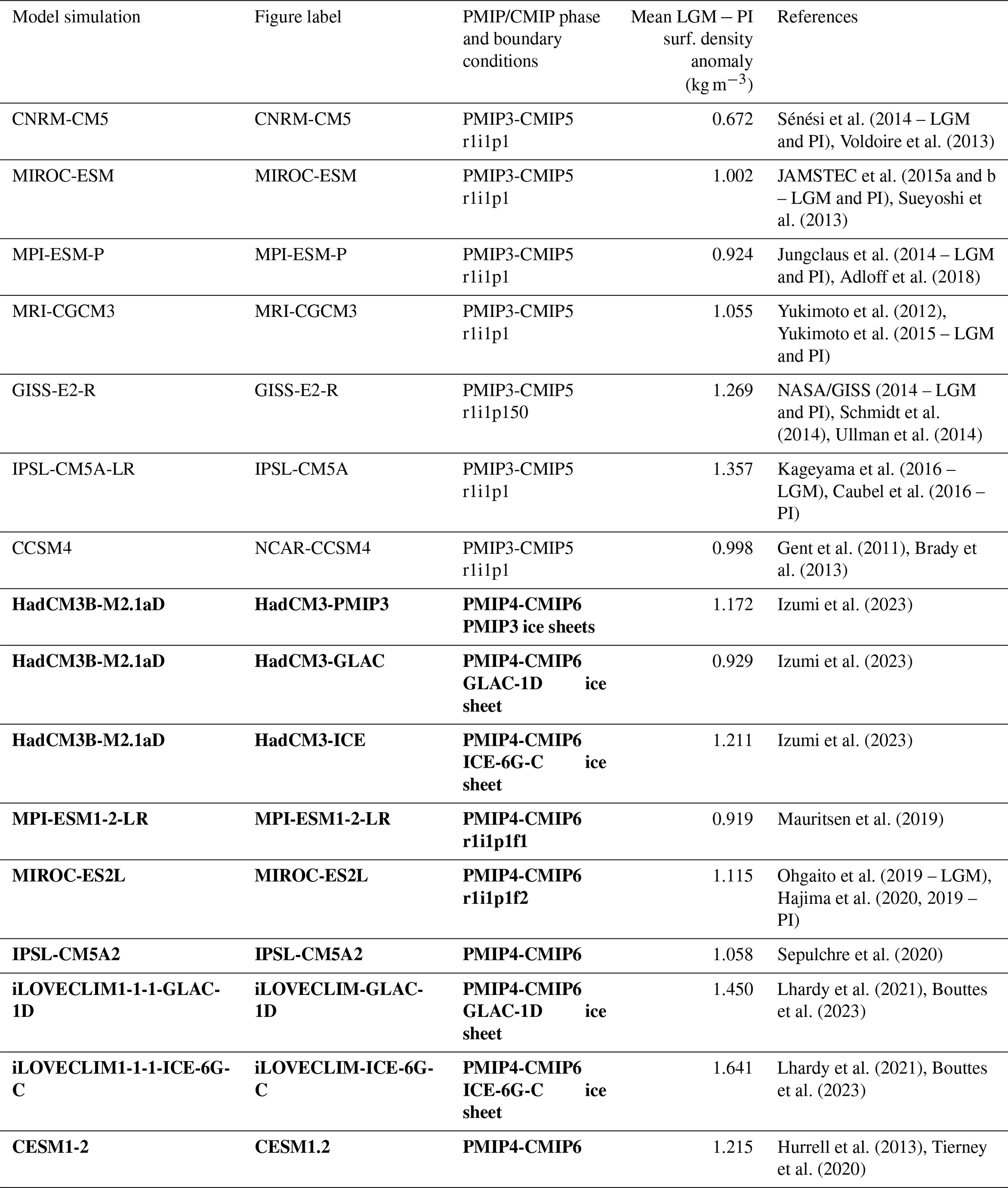
For this study, we used LGM and pre-industrial (hereafter piControl) climate model simulations from a total of sixteen simulations, including seven from PMIP3 (Braconnot et al., 2012) and nine from PMIP4 (Kageyama et al., 2018) (see Table 1). Two more simulations were excluded due to inconsistencies in salinity data (e.g., unit or formatting issues), making them unsuitable for analysis. Some model simulations share the same piControl but differ by their imposed ice-sheet reconstructions for LGM (e.g., HadCM3-ICE6GC vs. HadCM3-GLAC1D and iLOVECLIM1-1-1-GLAC1D vs. iLOVECLIM-1-1-1-ICE-6G-C). We tested whether simulations from the same model (within a PMIP phase or across PMIP3/PMIP4 versions) were too similar to each other. Our analysis showed that all simulations differed in at least one basin and for at least one of the variables (SSS, SST, density). Based on this, we retained all simulations.

The pre-industrial control simulation uses the constant boundary conditions established for 1850 CE (Eyring et al., 2016). It aims to produce a stable quasi-equilibrium climate under 1850 conditions, characterised by the annual cycle (mean and seasonality) and internal variability arising from interactions between Earth system components. This simulation serves as a baseline from which changes in all other experiments are calculated.

The LGM experimental protocol (Kageyama et al., 2017) considered as boundary conditions the large continental ice sheets, the associated land-sea mask changes, adjustments to ocean salinity (as ice sheets store large volumes of freshwater), and reductions in greenhouse gases. This makes it a challenging experiment for climate models, which explains why only a limited number of modelling groups have performed it. In two simulations (MIROC-ESM and IPSL-CM5A2), the salinity field was not initialized with the +1 psu offset prescribed in the protocol to account for freshwater stored in ice sheets. To ensure comparability across models, we added +1 psu to the LGM salinity of these two simulations before calculating absolute density. Here, “absolute” surface density refers to the full LGM density state, including the mean ocean density increase associated with reduced ocean volume and the corresponding global salinity offset prescribed by the LGM protocol. It therefore differs from the hydrographic density anomaly driven only by local changes in SST and SSS. To ensure comparability across simulations, we first place all model outputs on the same absolute-density baseline by applying the prescribed +1 psu correction where needed. Simulations performed with the iLOVECLIM model found the dynamical effect of that +1 psu to be very small, supporting this direct correction (Caley et al., 2026). For the calculation of surface density changes due to the hydrographic changes in SST and SSS, i.e. corrected for mean ocean density changes related to ocean volume, we removed this +1 psu from the LGM simulations and applied a −0.77 kg m⁻³ density correction to the reconstructions, following Caley et al. (2026).

We analysed annual mean SSS and SST from these simulations. All outputs were regridded to a common 1° × 1° grid, and monthly data were averaged to obtain climatological annual means. These means were computed over the full duration of each simulation, which ranges from 100 to 1100 years for the piControl experiments and up to 500 years for the LGM experiments.

The variables used here are salinity (so) and temperature (thetao). To study surface density, we used salinity and temperature from the first ocean layer. Seawater density was calculated using the gsw (Gibbs Seawater) Python package, which is based on the TEOS-10 thermodynamic framework and provides thermodynamically consistent equations for seawater properties. The gsw package requires Absolute Salinity (SA) and Conservative Temperature (CT) as inputs. CT is a more accurate and thermodynamically sound analog of Potential Temperature (θ), and SA is derived from Practical Salinity (SP), which is unitless and not directly usable in thermodynamic calculations. Since the model simulations originally provided SP and θ, we first converted them to SA and CT using the functions SA_from_SP and CT_from_pt, respectively. Finally, in-situ seawater density was computed with gsw.rho (SA, CT, p), using a computationally efficient expression for specific volume as a function of SA, CT, and pressure (Roquet et al., 2015).

Table 1 Model simulations available for this study, with LGM and piControl simulations. Model simulations from PMIP3 and PMIP4 (in bold) and mean LGM-PI surface density anomaly for each simulation (kg m⁻³). References correspond to the model description papers and/or ESGF simulation references when available.

2.3 Statistical analysis

Model–data comparisons were performed on a 1° × 1° grid, restricted to locations where proxy reconstructions provide valid values. Model anomalies were extracted exactly at the proxy sites to ensure strict spatial consistency. In this study, the term “anomaly” refers to the difference between two climatic states (LGM minus PI), following common usage in paleoclimate studies, and does not imply a deviation from a mean state.

Distributional agreement between models and reconstructions was evaluated using three complementary criteria. First, interquartile range (IQR) overlap was assessed to check distributional consistency while limiting sensitivity to extreme outliers. Second, the Kolmogorov–Smirnov (KS) statistic, which quantifies the maximal difference between cumulative distributions. At the global scale, the KS threshold is 0.13, consistent with the sample size of our dataset. A KS statistic below the threshold indicates that the model and reconstruction distributions are statistically consistent, whereas values exceeding the threshold indicate a significant difference between distributions. Third, a two-sample KS test p-value < 0.05 indicates a statistically significant difference between distributions: a value above 0.05 indicates that the null hypothesis of identical distributions cannot be rejected, while p< 0.05 indicates a significant difference. For visualization, kernel density estimates (KDEs) provided smoothed, continuous representations of the distributions, highlighting central tendencies and the most frequent values.

For the global density anomaly distribution analysis (Sect. 3.2), reconstruction uncertainty was additionally propagated using a Monte Carlo approach (10 000 iterations). For each reconstruction site, density anomalies were randomly sampled within their asymmetric 95 % confidence intervals derived from the Bayesian calibration model (Caley et al., 2026). The reconstructed median, interquartile range (IQR), and KS statistics were then recalculated for each realization. This procedure allowed us to evaluate how reconstruction uncertainty affects the distributional comparison between models and data.

For linear relationships, regression analyses were performed separately for PI and LGM periods. The coefficient of determination (R²) quantifies the proportion of variance in reconstructions explained by the models, while the slope measures the amplitude of the model response relative to observations. To account for uncertainties in the reconstructions, a Monte Carlo procedure (10 000 iterations) added Gaussian noise to the observations, derived from the 95 % confidence intervals. Distributions of R² and slope were then analyzed, and reported values correspond to mean ± standard deviation.

To further compare data and model simulations we introduce other metrics to reduce overreliance on regression and correlation. Root mean square error (RMSE) quantifies the average magnitude of errors between model and observations (lower values indicate better agreement), while bias measures the mean signed difference and thus highlights systematic over- or under-estimation (values close to zero are optimal). The Nash–Sutcliffe efficiency (NSE) evaluates the ability of model simulations to reproduce the observed variability. Values close to 1 indicate high skill, whereas negative values indicate poor model performance. The Kling–Gupta efficiency (KGE) combines correlation, variability, and bias into a single metric, providing an integrated measure of model performance, with values close to 1 indicating better agreement.

This framework provides a coherent and rigorous assessment of model-data agreement by combining distribution-based comparisons with analyses of linear relationships. It integrates multiple complementary metrics to evaluate performance, and accounts for reconstruction uncertainties through Monte Carlo approaches. Together, these methods offer a comprehensive evaluation of how well model simulations reproduce observed fields, both globally and across individual ocean basins.

2.4 Testing spatial representativeness with a pseudo-proxy approach

The spatial distribution of reconstructions is uneven, with a clear concentration of data near coastal areas (Figs. 1, S1 in the Supplement).

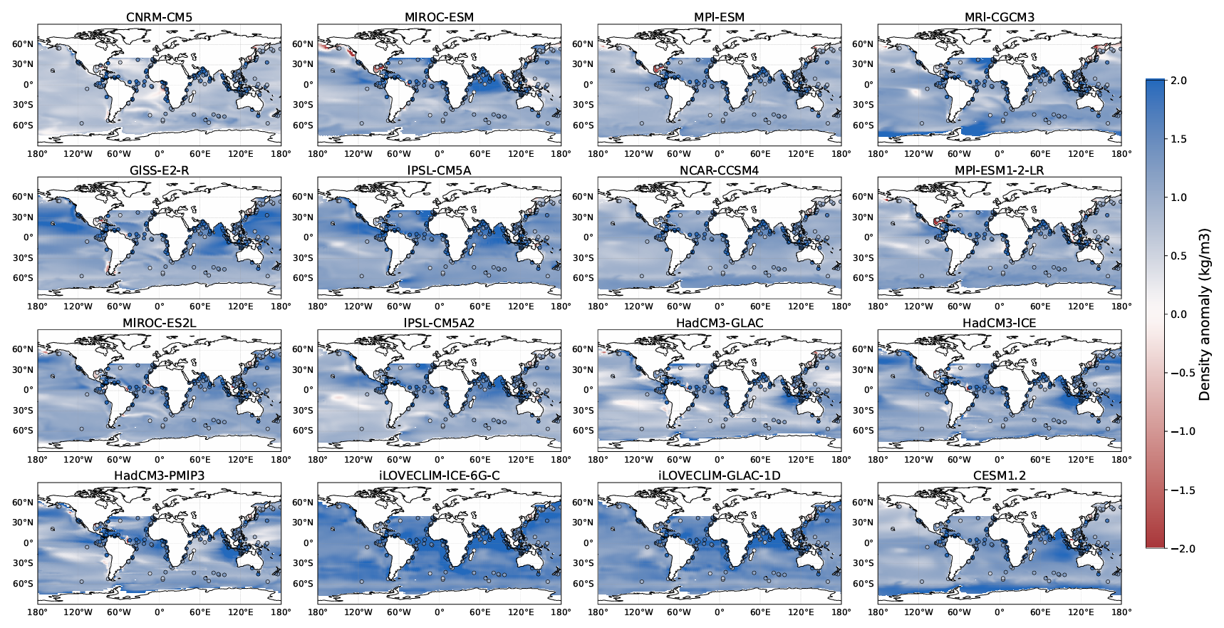
Figure 1 Absolute surface density (kg m⁻³) anomaly map (LGM − PIControl). The dots represent the surface density anomaly database reconstructions (Caley et al., 2026) and the background map is the anomaly mean for each model simulations in the study.

To assess whether the proxy data locations are representative of broader basin-scale conditions, a “pseudo-proxy” approach (Ayache et al., 2018) was performed, in order to compare the mean local values with basin-wide means derived from the models (Figs. 2, S2). Here, the pseudo-proxy approach does not refer to proxy system modelling or to the conversion of SST and SSS into a geochemical proxy signal. Instead, it is used as a spatial representativeness test: model values are sampled at the exact locations of the proxy reconstructions and compared with the basin-wide model mean. This allows us to assess whether the uneven proxy network provides an unbiased estimate of the large-scale basin signal. This analysis evaluates the spatial representativeness of proxy locations at the basin scale. However, it does not address differences between coastal and open-ocean environments, since climate models do not explicitly represent coastal processes and therefore cannot accurately simulate nearshore dynamics. Details on the basin definition and spatial masks used for this analysis are provided in Appendix A.

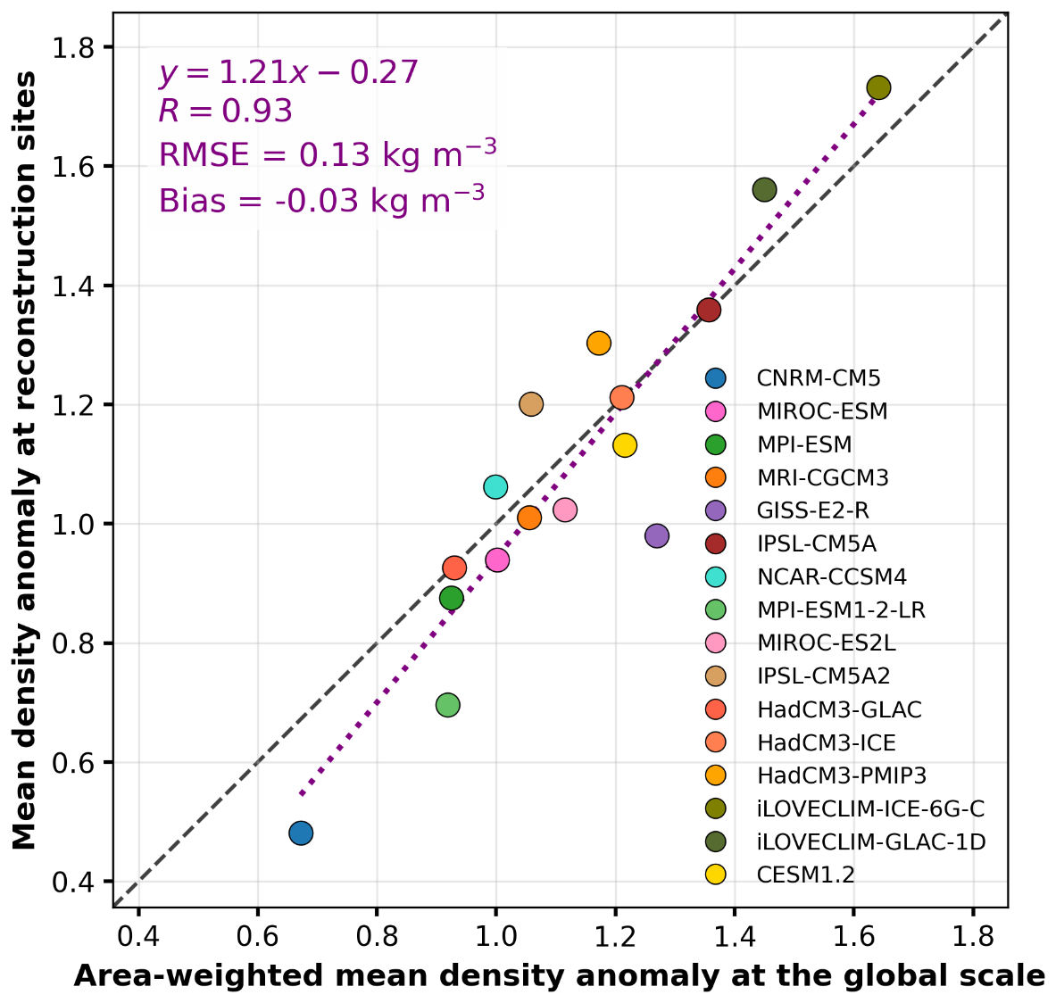
Figure 2 Pseudo-proxy test for global ocean surface density. Comparison between the mean density anomalies (kg m⁻³) averaged across all model grid points (x-axis) and the mean density anomalies (kg m⁻³) averaged over proxy reconstruction sites (y-axis). The purple regression line and R represent the fit across all model simulations (PMIP3 + PMIP4), with the corresponding root mean square error (RMSE) and bias also indicated. Results for individual basins are provided in Fig. S2.

For this purpose, we compare the average of density simulated by PMIP3 and PMIP4 model simulations over a given basin with the average density only at locations where proxy data are available (Figs. 2 and S2). A near-linear relationship is found at the global scale (Fig. 2) with the coefficient of correlation (R) at 0.93 and across most basins (Fig. S2), when compiling PMIP3 and PMIP4. These regressions indicate how well the mean over proxy sites reproduces the true basin-wide mean in the model simulations. The slopes being close to one and the high R values (p-value < 0.05), together with the low RMSE and bias values, indicate that the mean anomalies at the proxy sites capture the basin-wide means simulated by the models reasonably well. This suggests that, within the models, the uneven proxy distribution does not strongly bias the large-scale signal.

3 Evaluate model simulations at the global scale

Before investigating regional features, we first assess the large-scale behaviour of model simulations. A global-scale evaluation allows us to assess the overall ability of PMIP3 and PMIP4 simulations to reproduce the reconstructed large-scale signal of surface density changes between the LGM and the pre-industrial period. Evaluating models at this integrated scale also helps reduce the influence of local reconstruction uncertainties and highlights the dominant climatic drivers of density variations, such as global temperature and hydrological cycle changes.

3.1 Sea surface density anomaly (LGM − PI)

We first analyse absolute surface density anomalies between the LGM and the Pre-Industrial period (LGM − PI), in order to reduce the impact of potential systematic model-specific biases that may persist across time periods. All models simulate positive anomalies, i.e. they agree on the sign of the change. However, both the spatial patterns and the amplitude of the simulated anomalies vary considerably from one model simulation to another (Fig. 1). When averaged over space, simulated mean density anomalies typically range from 0.7 to 1.6, with an average value close to 1.1. In contrast, the proxy-based reconstructions exhibit a slightly higher mean, approximately 1.6.

When zonally averaged, the density anomaly (LGM − PI) in the observations (Fig. 3, grey dots) is stronger in the low latitudes than in the mid-latitudes, as already discussed in Caley et al. (2026). The observed increase in density during the LGM, both in the simulations and in the reconstructions, is consistent with the SST cooling (MARGO project, 2009; Tierney et al., 2020) and with a weaker hydrological cycle at low latitudes, in which precipitation decreased more than evaporation. This reduction in precipitation leads to saltier and denser surface waters (Kageyama et al., 2021), as already discussed in Caley et al. (2026).

Some model simulations fail to reproduce the full latitudinal structure, such as CNRM-CM5 and MPI-ESM-P, while others do not capture the shape but match the density anomaly well at low latitudes, for instance iLOVECLIM-ICE-6G-C and iLOVECLIM-GLAC-1D. Some model simulations, such as IPSL-CM5A and HadCM3-PMIP3, are in good agreement with the data across all latitudes, especially between 0 and 40° N, considering the uncertainties on the reconstructions (Fig. 3). The same type of zonally averaged analysis was performed for SSS (Appendix B) and for SSTs, the corresponding results are shown in Figs. B3 and B4 in Appendix B.

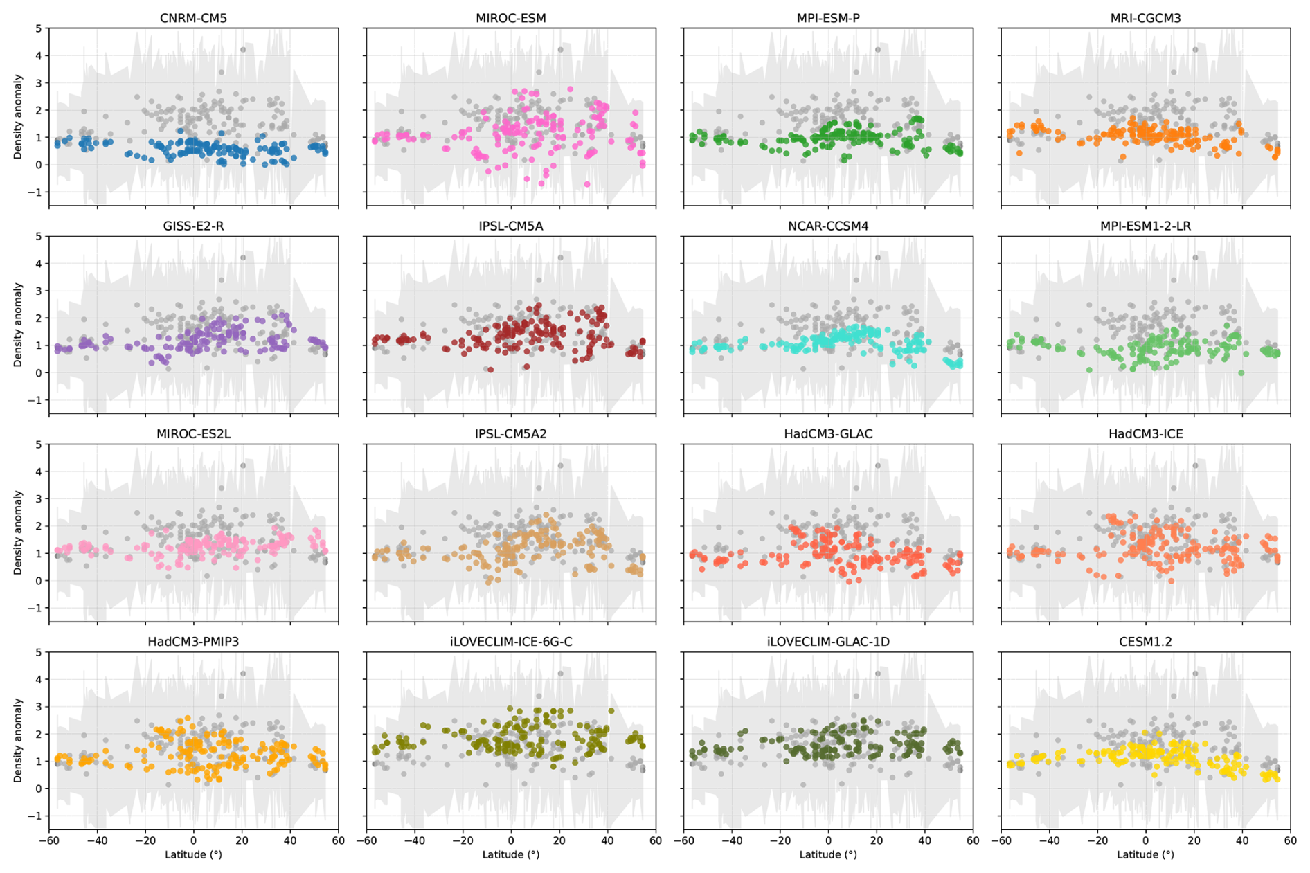
Figure 3 Density anomaly (kg m⁻³) as a function of latitude for each model simulation (colored dots) compared with the observational data (grey dots) and the 95 % confidence interval (grey shading). Model outliers, identified using the interquartile range (IQR) method (values outside 1.5 × IQR), were excluded to reduce the influence of extreme values. This filtering highlights the main structure and latitudinal patterns of the modelled density anomalies while retaining all available latitude points.

We next investigated the physical drivers of the density differences between reconstructions and simulations by decomposing the total density anomaly into temperature and salinity components. Model outputs and proxy datasets were collocated at common sampling points without additional interpolation, ensuring a strict one-to-one correspondence between density and SST observations. This procedure yielded 80 common points for the MARGO database (MARGO Project, 2009) and 92 points for the SST dataset from Tierney et al. (2020). No outlier filtering was applied.

Before computing the salinity contribution, the global density related to sea-level–induced salinity increase (−1 g kg⁻¹ in models, −0.77 kg m⁻³ in reconstructions; Caley et al., 2026) was removed to isolate density changes linked to hydrographic changes in SST and SSS. Because this correction is applied consistently to both reconstructions and model outputs, and since the analysis is based on model–data differences, it has no effect on the results presented here.

To quantify the relative influence of temperature and salinity on the model–data density anomaly differences, we decomposed the total density anomaly difference (model simulations minus reconstructions) into thermal and haline components using a Shapley decomposition. This approach accounts for the non-linearity of the seawater equation of state by averaging the contributions obtained from the two possible attribution sequences (temperature-first and salinity-first). The method provides an order-independent partitioning of the total density anomaly while ensuring that the sum of the thermal and haline contributions exactly reproduces the total density difference.

Figure 4 shows the relative contributions (%) of SST and salinity to the density anomaly difference for each model simulation. The relative importance of both components varies among simulations and between SST reconstruction datasets. For the MARGO-based estimates, SST and salinity contributions are often of comparable magnitude, whereas the Tierney-based estimates generally show a larger contribution from salinity. Nevertheless, SST effects alone cannot explain the differences in data-model density, demonstrating that hydrological changes substantially contribute to the differences in model-data density anomalies. It is also important to note that Fig. 4 presents basin-averaged contributions and therefore smooths part of the latitudinal variability observed in the density anomalies. The zonally averaged distributions shown in Fig. B2 (Appendix B) reveal that this spatial density (Fig. 3) variability is primarily controlled by salinity anomalies, whereas SST anomalies exhibit much weaker latitudinal variations across model simulations.

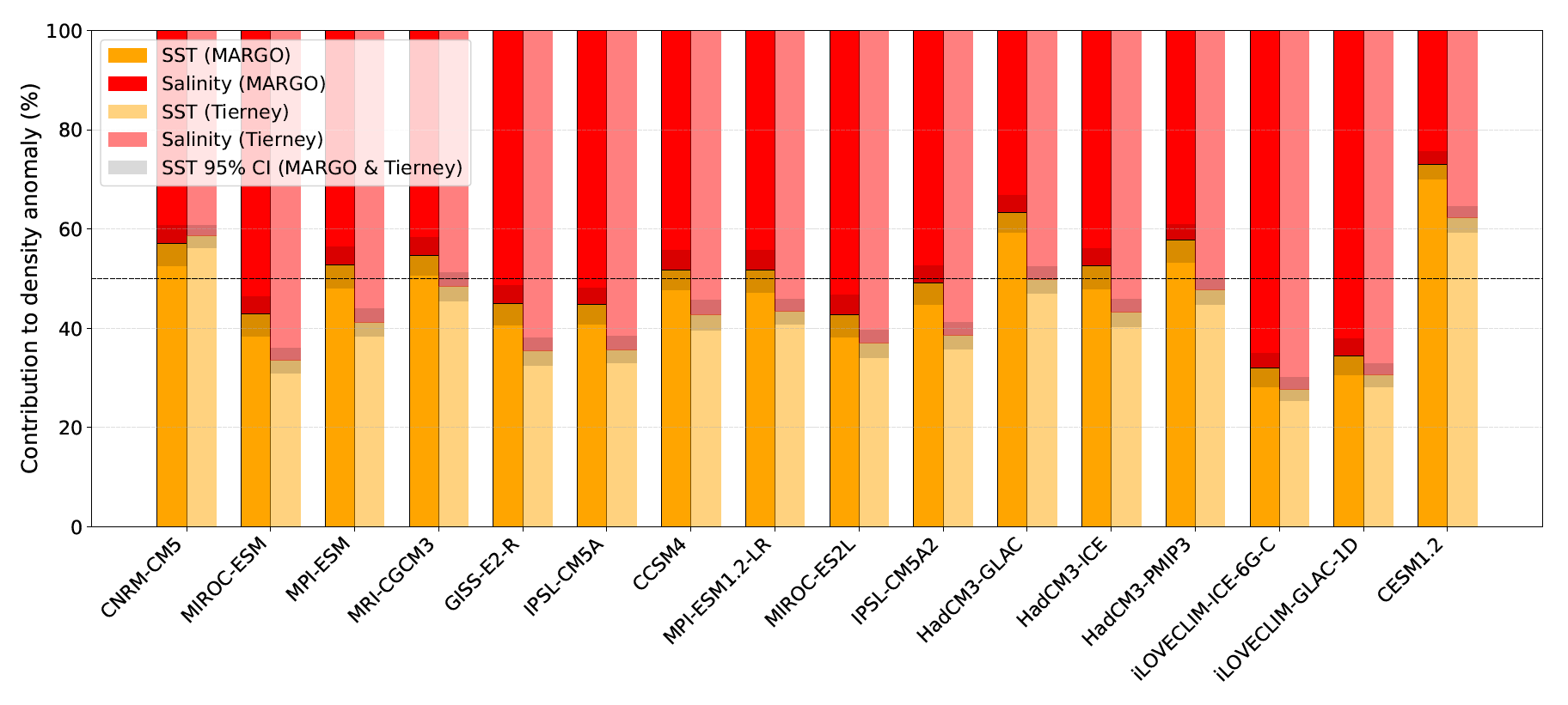
Figure 4 Relative contributions (%) of SST (orange) and salinity (red) to the model–data density anomaly differences (LGM − PI). Contributions were estimated using a Shapley decomposition, which provides an order-independent partitioning of density changes into thermal and haline components while accounting for the non-linearity of the seawater equation of state. Dark colours correspond to SST reconstructions from the MARGO Project (2009), whereas lighter colours correspond to Tierney et al. (2020). Shaded envelopes indicate the 95 % confidence intervals obtained by bootstrap propagation of SST reconstruction uncertainties.

Given that the hydrological cycle influences surface salinity and that salinity anomalies strongly influence the difference in data/model density anomalies, we explored the link between density anomalies and large-scale precipitation changes. Using the PMIP3 and PMIP4 ensembles, Kageyama et al. (2021) showed that nearly all models simulate substantial decreases in precipitation in high-rainfall regions during the LGM, particularly across the tropics and monsoon zones, although the magnitude varies between model simulations. Model simulations that best reproduce the density anomalies inferred from proxy data also tend to exhibit the largest reductions in tropical precipitation. In contrast, models with smaller precipitation decreases fail to reproduce the observed density structure. Figure 5 illustrates the relationship between density anomalies and mean annual precipitation anomalies for both the tropics (30° S–30° N, circle) and the global ocean (square). A clear linear relationship emerges between density anomalies and precipitation anomalies, with R²= 0.67 in the tropics and R²= 0.64 globally, highlighting the robustness of this connection (p-value < 0.05). This analysis emphasizes that accurately representing low-latitude hydrological feedbacks is critical for capturing the full magnitude of glacial ocean density changes.

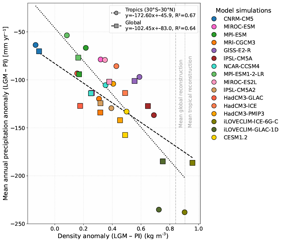
Figure 5 Mean annual precipitation anomalies (LGM − PI, mm yr⁻¹, over land and ocean) as a function of seawater density anomalies corrected for mean ocean density changes (kg m⁻³) relative to sea level-induced salinity increase at LGM. Scatter points show the relationship for the tropics (30° S–30° N, circle) and the global ocean (square). Dashed lines indicate linear regressions for each region, with the corresponding slope, intercept, and R². Precipitation anomalies are from Kageyama et al. (2021). Grey dashed lines indicate the mean tropical and global reconstructions. No linear relationship is found between SST anomalies and mean annual precipitation anomalies (not shown), indicating that the link between density anomalies and precipitation is primarily driven by salinity changes.

In summary, our results indicate that SST effects alone cannot explain the density anomaly differences between reconstructions and simulations. Instead, salinity differences account for most of the model–data anomaly density discrepancy (Fig. 4) and are directly linked to reductions in tropical precipitation. Models that simulate stronger tropical precipitation decreases reproduce the observed LGM surface density anomalies more accurately, emphasizing the importance of representing low-latitude hydrological feedbacks to capture the full magnitude of glacial ocean density changes.

3.2 Comparison of global distribution of surface density anomalies

Before analysing regional contrasts, we first evaluate model performances considering the global distribution of absolute surface density anomalies (LGM − PI) by aggregating data from all selected ocean basins (Figs. 6, 7 and C1 in Appendix C).

Model-data agreement was evaluated using three complementary statistical criteria (see Sect. 2.2): a Monte Carlo-derived p-value > 0.05 from a two-sample Kolmogorov-Smirnov (KS) test, a Monte Carlo-derived KS statistic below 0.13 and overlapping interquartile ranges (IQRs) between data and model distributions, indicating consistent variability. Together, these criteria evaluate whether models reproduce not only the central value but also the overall shape of the reconstructed distribution.

Figure 6 visually illustrates these three criteria through the coloured flags, which show whether the Monte Carlo-derived KS statistic, p-value, and IQR criteria are satisfied for each model simulation. Figure 7 complements this by showing only the IQR and median values of the model and reconstruction distributions, including a Monte Carlo propagated reconstruction uncertainty, allowing a direct comparison of central tendency and spread.

Reconstruction-based anomalies have a median value of 1.19, whereas the values obtained from model simulations vary widely, ranging from 0.6 to 1.6 (Figs. 6 and C1). Interquartile ranges (IQRs) support this divergence. Using the reconstruction values without considering reconstructions uncertainties, the reconstructions exhibit a broader spread (IQR ∼0.75), while models show smaller variability (IQR between 0.27 and 0.98). However, when reconstruction uncertainties are propagated through the Monte Carlo procedure, the reconstructed IQR increases substantially, reflecting the uncertainty associated with the density calibration. As a result, all model simulations fall within the Monte Carlo-derived reconstruction IQR envelope (Figs. 6 and 7), indicating that differences in distributional spread alone are no longer sufficient to discriminate between simulations. Once reconstruction uncertainty is propagated, the IQR criterion is satisfied by all simulations, leaving the Monte Carlo-derived KS statistic and associated p-value as the main metrics discriminating among model simulations.

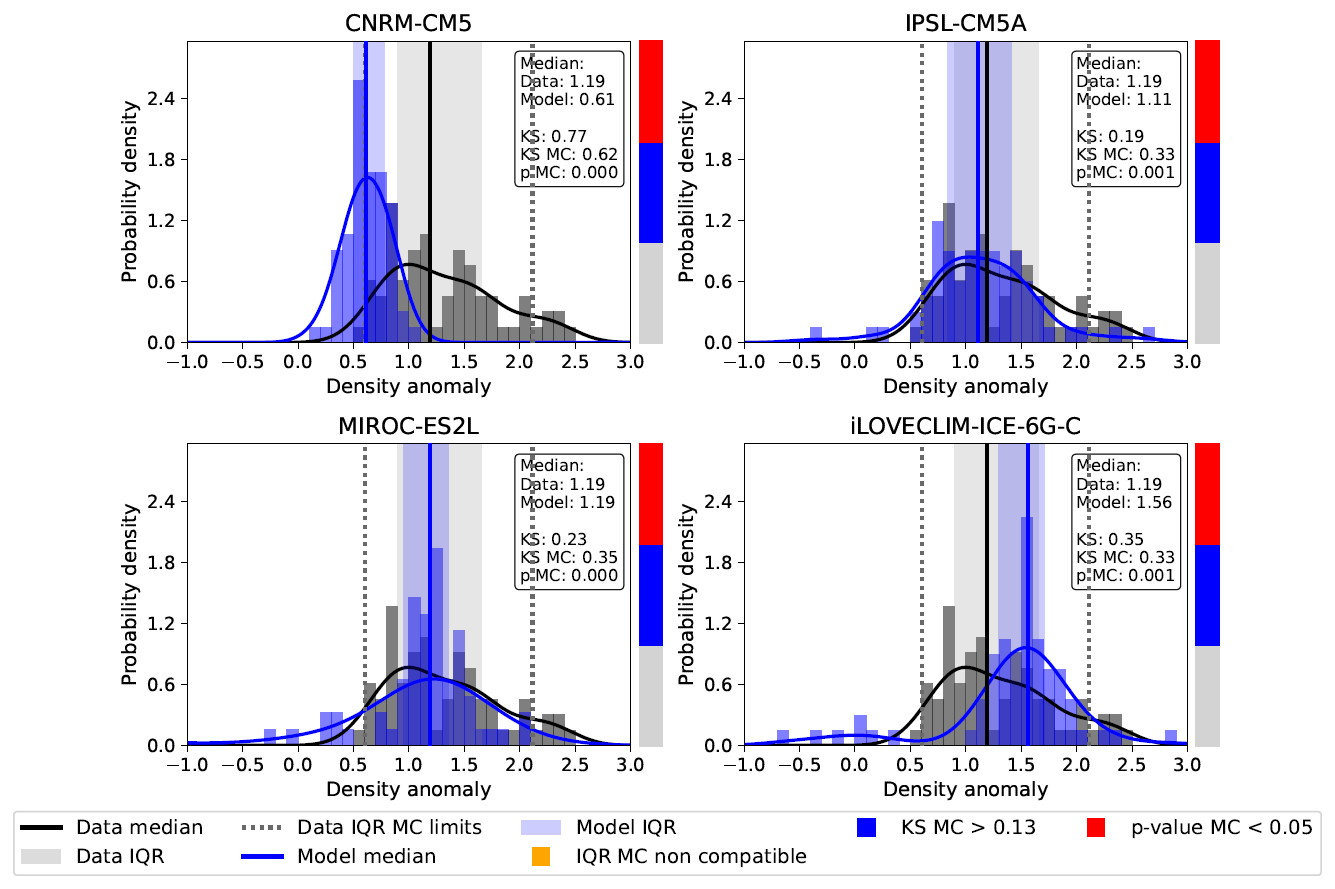
Figure 6 Distribution histograms of surface density anomalies (LGM − PI, kg m⁻³) for an example of four model simulations. Density reconstructions are shown in black, model simulations in blue. Kernel Density Estimates (KDEs) illustrate the central tendency and overall shape of the distributions. Vertical lines indicate the median of each distribution, and shaded envelopes represent the interquartile ranges (IQRs), providing a measure of data spread that is independent of extreme values. Grey dotted lines indicate the limits of the Monte Carlo propagated reconstruction IQR obtained after accounting for the 95 % confidence intervals associated with the density reconstructions. The histograms display the frequency of values, complementing the KDEs and IQRs to give an integrated view of distribution characteristics. Reconstructions uncertainties are explicitly propagated through the Monte Carlo procedure. Colored indicators on the right side of each panel summarize the outcomes of the three comparison metrics. A red flag indicates a Monte Carlo-derived two-sample KS test with p< 0.05, a blue flag indicates a Monte Carlo-derived KS statistic exceeding the global critical threshold (KS > 0.13), and an orange flag indicates non-overlapping Monte Carlo propagated IQRs between reconstructed and simulated distributions.

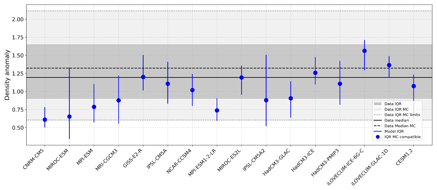
Figure 7 Comparison of observed and simulated density anomaly statistics at the global scale. The dark grey band indicates the reconstructed IQR without considering uncertainties, while the light grey band and grey dotted lines indicate the Monte Carlo propagated reconstruction IQR after accounting for reconstruction uncertainty. The solid black line marks the reconstructed median and the dashed black line the Monte Carlo median. For each model simulation, the blue vertical bars represent the modelled IQR, while the circular markers represent the model median. Blue markers indicate model simulations with IQR values consistent with the Monte Carlo propagated reconstruction IQR.

As shown in Figs. 6 and 7, none of the simulations satisfy all three criteria simultaneously. Although all simulations satisfy the IQR criterion, all Monte Carlo-derived KS statistics remain above the prescribed threshold (0.13) and all Monte Carlo-derived p-values remain below 0.05. This indicates that, although the observed range of variability can be reconciled once reconstruction uncertainty is considered, important discrepancies persist in the overall shape of the modelled and reconstructed distributions. Consequently, agreement between reconstructed and simulated global distributions remains limited.

Because density anomalies depend on both temperature and salinity, we also compared the distribution of SST anomalies between models and reconstructions using the MARGO (MARGO project, 2009) and Tierney et al. (2020) datasets (Figs. S3 and S4). Using the MARGO (MARGO project, 2009) reconstructions, 14 out of 16 simulations (81 %) satisfy the Monte Carlo propagated IQR criterion, indicating that model and proxy interquartile ranges remain largely consistent after accounting for reconstruction uncertainty. However, all Monte Carlo-derived KS statistics remain above the prescribed threshold and all Monte Carlo-derived p-values remain below 0.05, indicating that although the overall spread of modelled and reconstructed SST anomalies is comparable, their overall distribution remain statistically different.

Similarly, for the Tierney et al. (2020) dataset, 14 out of 16 simulations (87.5 %) satisfy the Monte Carlo propagated IQR criterion and 1 out of 16 simulations satisfy the MC p-value limit. For the MARGO comparison, all Monte Carlo-derived KS statistics exceed the prescribed threshold and all Monte Carlo-derived p-values remain below 0.05, indicating that none of the simulations reproduce the overall distribution of reconstructed SST anomalies despite generally consistent interquartile ranges.

Finally, part of the mismatch may arise from the uneven spatial distribution of reconstructions, which are mostly located near coastal areas (Fig. 1). These coastal regions are particularly complex to simulate due to influences such as continental runoff and oceanic upwelling, which are often poorly captured by global climate models. Consequently, kernel density estimates derived from reconstructions appear flatter, suggesting greater variability not captured by the models. Additionally, reconstructions in some key upwelling zones remain problematic, as highlighted by Caley et al. (2026), further complicating the comparison and evaluation of model outputs against data.

3.3 Global evaluation of surface density: models vs. reconstructions (PI and LGM)

One limitation of working with anomalies is that any observed difference between data and model simulations in absolute surface density cannot be directly linked to either the LGM or the PI baseline. To address this, we analysed the two periods separately, the LGM and the PI, as shown in Figs. 8 and 9.

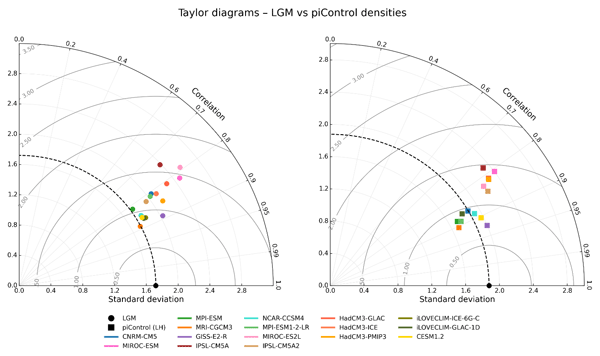
Model simulations performance was evaluated using Taylor diagrams (Fig. 8), which summarize the spatial correlation, normalized standard deviation and centered root-mean-square error (CRMSE) between simulated and reconstructed surface densities, together with complementary statistical metrics (RMSE, bias, NSE and KGE; Fig. 9). This multi-metric approach provides a more comprehensive assessment of model skill by simultaneously evaluating the spatial pattern, variability, systematic bias and overall agreement with the reconstructions.

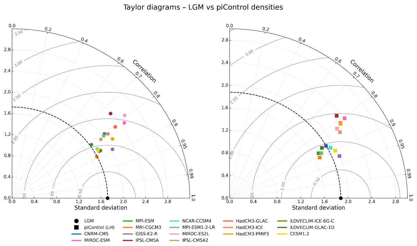
Figure 8 Taylor diagrams comparing model simulations performance for LGM (left) and piControl (LH, right) ocean surface density reconstructions. All grid cells are equally weighted in these diagrams. Each point represents a climate model simulation. Circles correspond to the Last Glacial Maximum (LGM), while squares correspond to the pre-industrial control simulation (piControl, LH). The radial distance indicates the model simulation standard deviation, while the angular coordinate represents the pattern correlation between model outputs and reconstructions. The black dots define the reference observational standard deviation which represents the spatial variability of the observational reconstructions, computed as the standard deviation of all observations within each period. Contours show centered root-mean-square error (CRMSE) relative to observations.

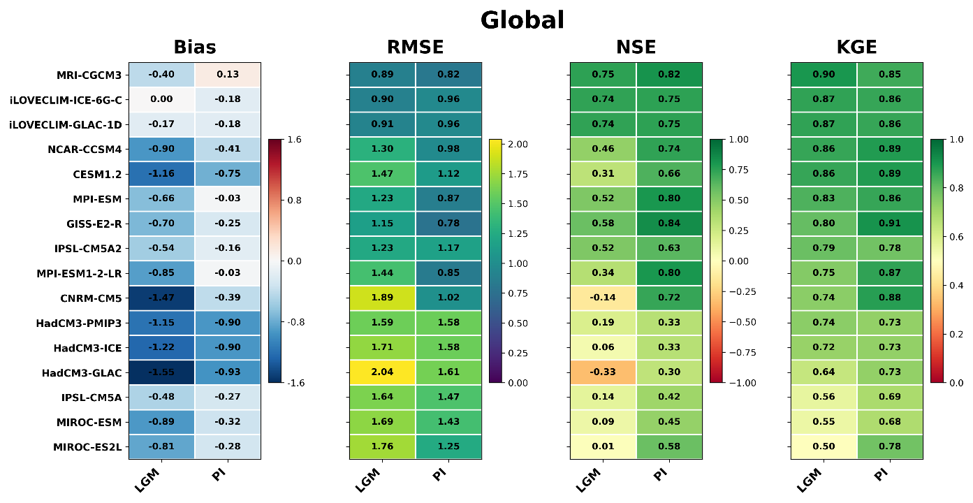
Figure 9 Global model simulations performance for sea surface density during the LGM and PI periods. Heatmaps show four complementary metrics calculated from model–data comparisons at reconstruction grid cells common to all simulations: bias, root mean square error (RMSE), Nash–Sutcliffe efficiency (NSE), and Kling–Gupta efficiency (KGE). For bias and RMSE, values close to 0 indicate better agreement, whereas for NSE and KGE, values close to 1 indicate higher skill. Negative NSE values indicate poor model performance. Models are ranked according to their LGM KGE values. For each metric, LGM and PI are shown side by side using the same colour scale, allowing direct comparison of model performance between climatic periods.

Overall, the Taylor diagrams (Fig. 8) and the complementary performance metrics (Fig. 9) provide a consistent assessment of model simulations skill. During the LGM, the two iLOVECLIM simulations remain among the best-performing model simulations, combining the lowest RMSE values (0.90–0.91 kg m⁻³), high NSE values (0.74), and KGE values of 0.87, while also exhibiting excellent agreement in the Taylor diagram. MRI-CGCM3 performs similarly well, with the highest KGE (0.90), a low RMSE (0.89 kg m⁻³), and a relatively small bias (−0.40 kg m⁻³). IPSL-CM5A2 and MPI-ESM also rank among the strongest simulations, indicating that several model simulations reproduce both the spatial variability and the magnitude of reconstructed surface densities with good overall skill. Rather than identifying a single best-performing simulation, the different metrics consistently highlight a small group of high-performing model simulations.

In contrast, HadCM3-GLAC, HadCM3-ICE, HadCM3-PMIP3 and MIROC-ESM consistently rank among the least skilful simulations. These model simulations combine relatively large RMSE values, pronounced negative biases, lower correlations in the Taylor diagrams, and reduced NSE and KGE values, indicating persistent difficulties in reproducing the mean state, the amplitude of spatial variability, and the spatial pattern of reconstructed surface densities. These differences are also evident in the regression plots (Fig. D1 in Appendix D), where the best-performing model simulations display data points clustered close to the 1 : 1 line, whereas poorer-performing simulations exhibit larger scatter and systematic departures from this relationship.

A similar overall hierarchy is observed for the PI simulations. The two iLOVECLIM experiments again remain among the best-performing model simulations, exhibiting low RMSE values (0.96 kg m⁻³), high NSE values (0.75), and KGE values of 0.86. However, MRI-CGCM3, GISS-E2-R, MPI-ESM and NCAR-CCSM4 achieve comparable performance depending on the metric considered. In particular, GISS-E2-R reaches the highest KGE (0.91), while MRI-CGCM3 shows the highest NSE (0.82), illustrating once again that no single simulation systematically outperforms all others across every evaluation metric.

The HadCM3 simulations and MIROC-ESM remain among the poorer performing during the PI, exhibiting the largest RMSE values together with comparatively low NSE and KGE values, although their performance is generally improved relative to the LGM.

Compared with the LGM, most simulations exhibit improved scores during the PI, particularly in terms of NSE and KGE, suggesting that reproducing the pre-industrial mean state, the amplitude of spatial variability, and the spatial pattern of surface density is generally less challenging than under glacial boundary conditions. Nevertheless, the relative hierarchy among the best- and worst-performing simulations remains broadly consistent between the two periods.

The bias metric further highlights systematic differences among simulations. Most model simulations exhibit negative biases during both periods, indicating a general tendency to underestimate reconstructed surface densities. This behaviour is particularly pronounced for the HadCM3 simulations during both periods and for CNRM-CM5 during the LGM. MRI-CGCM3 is the only simulation displaying a slight positive bias during the PI (+0.15 kg m⁻³). These systematic offsets indicate that several simulations reproduce the large-scale spatial structure of surface density reasonably well while still underestimating its absolute values.

None of the simulations can be considered wholly inadequate, as all exhibit KGE values of at least ≃ 0.5, reflecting a moderate to good overall representation of the reconstructed surface densities. The global evaluation nevertheless masks important regional contrasts. We therefore examine in the following section whether the agreement identified here is maintained across the different ocean basins.

4 Evaluate model simulations at regional scale: focus on the Indian Ocean

Despite global-scale agreement between reconstructions and simulations, the mismatches observed in the statistical metrics reveals that key patterns are not captured. This motivates a basin-by-basin analysis to better understand the regional origins of these discrepancies.

We created 8 ocean basins masks (see Appendix A). To evaluate model performance within coherent oceanographic regions while accounting for the latitudinal structure identified in the global analysis, oceans were subdivided into northern and southern sectors (Appendix A). In the following, we focus the main discussion on the Indian Ocean. This choice is motivated by the central role of the Indian Ocean in tropical–extratropical interactions and its importance for major hydroclimate processes such as the monsoon and Walker circulation dynamics. Previous studies have already conducted data–model comparisons in this region, revealing its complexity.

Analyses of the other ocean basins are provided in the Supplement (Figs. S5, S6 and S7) using three statistical metrics (R, RMSE and Bias). Detailed analyses of these ocean basins will be for future studies but, briefly, performance of the data model comparison is variable depending of the ocean basin and simulations considered. The South Atlantic and North Pacific (north of 40° N) ocean basins indicate the highest bias and RMSE and lowest correlation for weighted averages simulations.

Regional model simulations performance for the Indian Ocean basin is evaluated using complementary skill metrics (Bias, RMSE, NSE and KGE), providing a more direct assessment of model–data agreement.

4.1 Evaluation of model simulations performance in the North and South Indian Ocean

The Indian Ocean is divided into two dynamically distinct regions separated at the Equator (0°). The southern basin extends to 40° S, approximately corresponding to the present-day subtropical convergence and the southern limit of the Agulhas current system. This subdivision isolates the monsoon-dominated North Indian Ocean from the subtropical South Indian Ocean, allowing us to evaluate model performance in two contrasting dynamical regimes. As for the global data-model comparison, model simulation skill is assessed using four complementary metrics computed from reconstructed and simulated surface density fields: Root Mean Square Error (RMSE), Bias, Nash–Sutcliffe Efficiency (NSE) and Kling–Gupta Efficiency (KGE). During the LGM (Fig. 10), weighted KGE values indicate that almost all simulations provide a satisfactory representation of reconstructed Indian Ocean surface density. Although some differences exist among model simulations, they remain relatively limited, suggesting broadly comparable overall performance across most simulations. In contrast, the two iLOVECLIM simulations clearly stand apart, exhibiting markedly lower KGE values and substantially poorer agreement with the reconstructions. This contrasts with their strong performance in the global LGM and PI evaluations (Fig. 9), where the two iLOVECLIM simulations ranked among the best-performing model simulations. This discrepancy highlights the regional dependence of model–data agreement and suggests that good global performance can mask substantial regional differences.

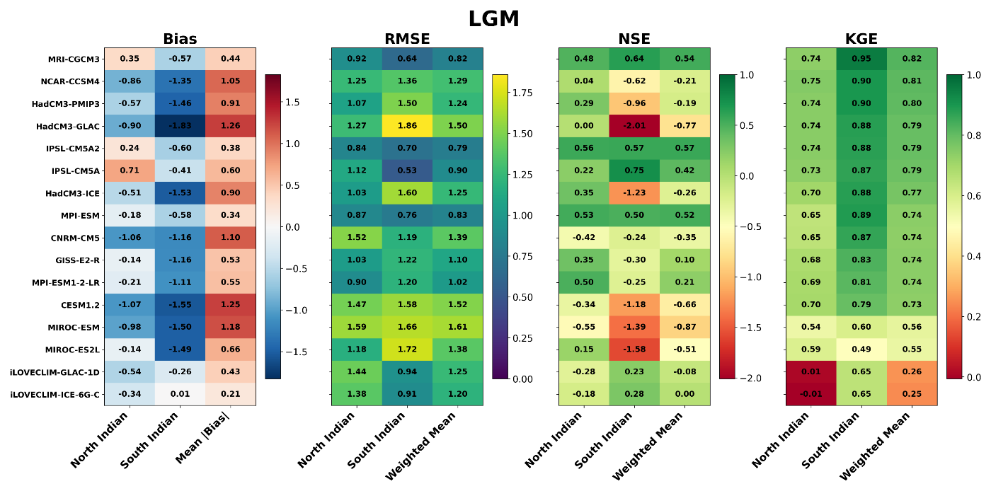
Figure 10 Simulations performance for seawater density in the North Indian and South Indian oceans during the Last Glacial Maximum (LGM). Heatmaps show four complementary performance metrics calculated from model–data comparisons at proxy reconstruction sites. Model simulations are ranked according to their weighted mean Kling–Gupta Efficiency (KGE), averaged across both basins. The metrics shown are: mean absolute bias (|Bias|), root mean square error (RMSE), Nash–Sutcliffe efficiency (NSE), and Kling–Gupta efficiency (KGE). For each simulation, the weighted mean values were computed using the number of valid grid points available within each basin. Lower values of |Bias| and RMSE indicate better agreement with the reconstructions, with values close to 0 being optimal, whereas higher values of NSE and KGE indicate better model performance, with an optimum value of 1. Negative NSE values indicate poor model performance.

This overall picture remains consistent when considering the two basins separately. KGE values are generally higher in the South Indian Ocean than in the North Indian Ocean, indicating that reconstructed density patterns are more readily reproduced in the southern Indian Ocean. Once again, the two iLOVECLIM simulations are ranked lower compare than the other simulations, particularly in the North Indian Ocean, where their KGE values approach zero. The particularly poor performance of iLOVECLIM in the North Indian Ocean likely contributes to the contrast between its global and regional skill. Because the global evaluation combines information across the entire ocean domain, strong performance in other regions may compensate for poorer agreement in the Indian Ocean.

The remaining metrics provide complementary information on different aspects of model simulations performance and broadly support the KGE assessment. Simulations associated with relatively high KGE values generally also exhibit low RMSE values, indicating limited overall model–data differences, while absolute biases remain moderate although somewhat more variable among simulations. NSE highlights larger differences in the overall agreement between simulations and the reconstructed density field, owing to its sensitivity to both variability representation and large errors. In particular, several HadCM3 simulations exhibit relatively low or even negative NSE values in the South Indian Ocean despite maintaining relatively high KGE values. This suggests that, while the simulations achieve good overall agreement with the reconstructed density field, they are affected by error structures that are more strongly penalized by the NSE than by the KGE. Conversely, the iLOVECLIM simulations display only moderate RMSE values but consistently low NSE and KGE values, highlighting that reproducing the overall magnitude of model–data differences alone is insufficient to ensure satisfactory overall model performance.

During the PI (Fig. 11), the results remain very similar to those obtained for the LGM. Most simulations again exhibit relatively high weighted KGE values, indicating satisfactory agreement with the reconstructed density field. Differences among simulations remain modest, whereas the two iLOVECLIM simulations once more stand apart, exhibiting negative KGE values that indicate a systematic inability to reproduce the reconstructed density field.

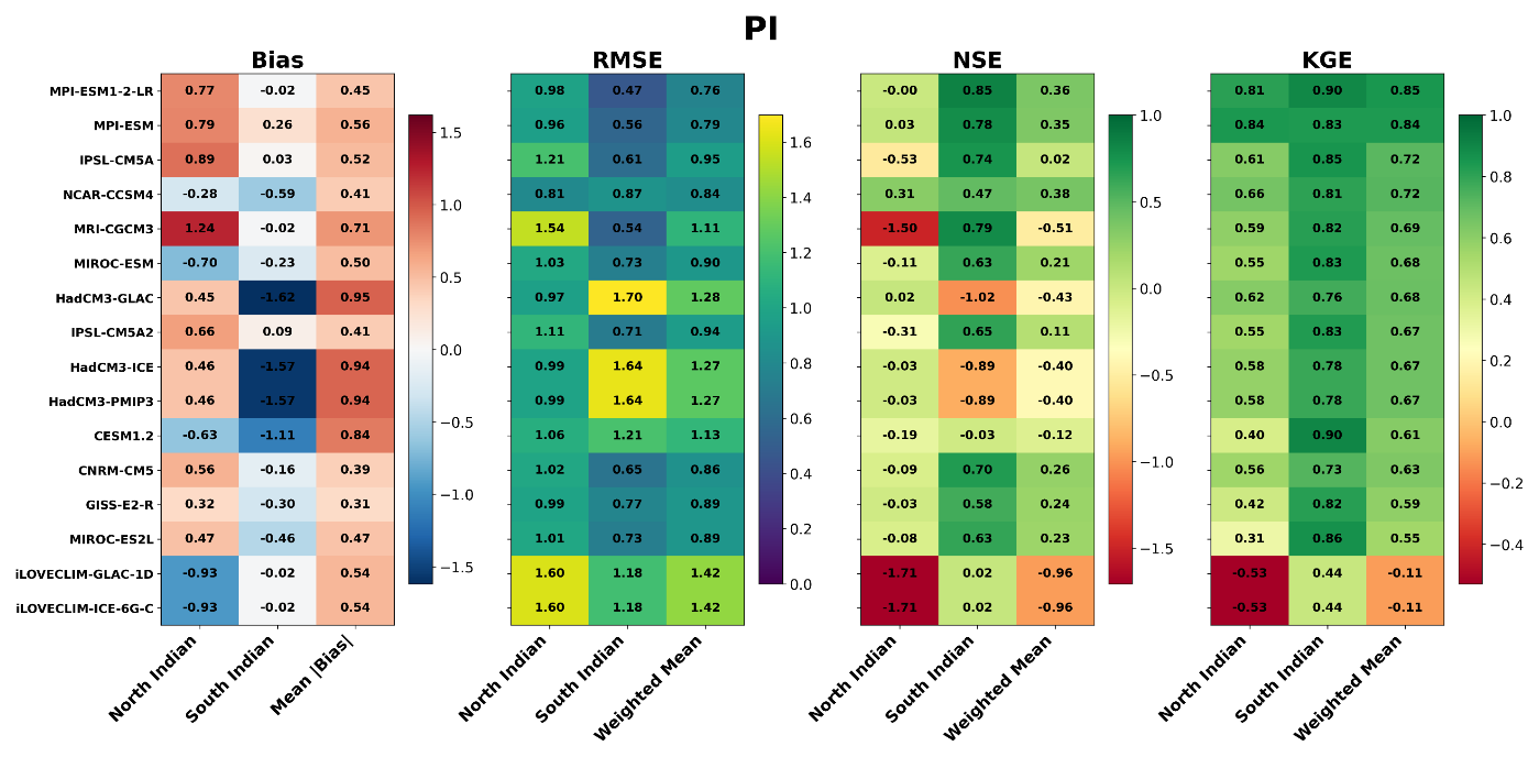
Figure 11 Simulations performance for seawater density in the North Indian and South Indian oceans during the pre-industrial period (PI). Heatmaps show four complementary performance metrics calculated from model–data comparisons at proxy reconstruction sites. Model simualtions are ranked according to their weighted mean Kling–Gupta Efficiency (KGE), averaged across both basins. The metrics shown are: mean absolute bias (|Bias|), root mean square error (RMSE), Nash–Sutcliffe efficiency (NSE), and Kling–Gupta efficiency (KGE). For each simulation, the weighted mean values were computed using the number of valid grid points available within each basin. Lower values of |Bias| and RMSE indicate better agreement with the reconstructions, with values close to 0 being optimal, whereas higher values of NSE and KGE indicate better model performance, with an optimum value of 1. Negative NSE values indicate poor model performance.

The north–south contrast observed during the LGM persists during the PI. Most simulations achieve higher KGE values in the South Indian Ocean than in the North Indian Ocean, confirming that reconstructed density fields are more readily reproduced in the south. As during the LGM, the two iLOVECLIM simulations are ranked lower compare than the other simulations, with negative KGE values in the North Indian Ocean.

RMSE, Bias and NSE support the same overall interpretation while highlighting complementary aspects of model simulations performance. Overall, the four complementary metrics consistently show that most simulations reproduce reconstructed Indian Ocean surface density reasonably well during the PI, whereas the two iLOVECLIM simulations exhibit consistently poor performance across all metrics.

4.2 The Indian Ocean West-East gradient

Beyond the North–South comparison presented in Sect. 4.1, one of the dominant modes of variability in the tropical Indian Ocean is characterized by a zonal rather than meridional structure and is most strongly expressed at interannual timescales. The Indian Ocean region, including part of the Indo-Pacific Warm Pool (IPWP), plays a critical role in the global climate system due to strong coupling between ocean and atmosphere, particularly through the Indo-Pacific Walker circulation. This circulation influences the zonal distribution of SST and thermocline depth, providing the background conditions for phenomena such as the Indian Ocean Dipole (IOD) (Saji et al., 1999; Abram et al., 2020). The Indian Ocean is also closely linked to the monsoon hydrological cycle, with precipitation patterns affecting surface salinity and, consequently, density, making it particularly sensitive to both temperature and salinity variations. However, climate models often misrepresent the mean state of the IOD, potentially leading to biases in simulating climate variability (Weller and Cai, 2013; Cai and Cowan, 2013). Notably, Abram et al. (2020) report that many models produce an overly strong thermocline-SST feedback due to a misrepresentation of the mean state, particularly an exaggerated zonal thermocline slope, which artificially increases the strength and frequency of simulated IOD events. Although research on the IOD has expanded over the past two decades, uncertainties remain regarding the controls and long-term evolution of the Indian Ocean's mean state, especially under different climate boundary conditions. The limited timeframe of the instrumental record and persistent model biases make paleoclimate reconstructions essential for investigating past mean states and for testing model performance beyond the range of modern variability (Abram et al., 2020). To date, paleoclimate data of SST suggest that past periods, such as during the LGM, mid-Holocene or 17th century, tend to have a mean state that is more typical of a positive IOD-like, which is systematically associated with elevated IOD variability. This indicates a tight coupling between the mean state and interannual dynamics (Abram et al., 2020).

Following the basin-scale evaluation presented in Sect. 4.1, we now investigate whether the observed model–data discrepancies originate from an incorrect simulation of the tropical West–East density gradient. To do so, model performance is evaluated using a West–East density gradient specifically designed to capture the mean-state structure associated with IOD-like conditions. SST and precipitation driving SSS changes create a West-East surface salinity gradient (Fig. 12) and therefore a density gradient. Recent observations show that, at interannual timescales, SSS variability is strongly linked to the IOD and ENSO, and can interact with SST anomalies through a SST–precipitation–SSS feedback. This suggests that SSS may at times amplify rather than offset SST-related changes (Zhang et al., 2016).

In this section, the “iLOVECLIM-ICE-6G-C” and “iLOVECLIM-GLAC-1D” simulations have been excluded due to a salinity bias in the northern Indian Ocean region caused by excess precipitation that reduces salinity in the iLOVECLIM model in comparison to reconstructions as shown by Roche and Caley (2013) and as confirmed by skill metrics for the Indian Ocean on Figs. 10 and 11.

Two boxes were defined: “Indian West”, which contains 6 density reconstructions and “Indian East”, which contains 5. These boxes were chosen based on the definition of the IOD by Saji et al. (1999), and slightly adjusted to ensure sufficient points within each box. Unlike the regional North–South boxes used elsewhere in this study, these boxes intentionally straddle the Equator because they are designed to capture the tropical zonal structure of the Indian Ocean Dipole rather than hemispheric contrasts. The “Indian West” box is defined as 50–70° E, 12° S–12° N, corresponding to the tropical western Indian Ocean. The “Indian East” box is defined as 90–110°E, 10° S–2° N, corresponding to the tropical south-eastern Indian Ocean. For model–data comparisons, model values are extracted at the exact grid cells where reconstructions are available. The SST points used by Tierney et al. (2020) in the “Indian East” box are geographically close to the density reconstructions, which favours a tighter spatial match between SST and density data. In contrast, reconstructions from the MARGO (MARGO project, 2009) database in the “Indian West” box are located farther offshore, showing less spatial overlap with the available density reconstructions.

Before analyzing the LGM–piControl difference, we verified that model simulations reproduce the West–East gradient observed during the pre-industrial period. To do this we compared the West–East gradient of SST, salinity, and surface density from each piControl simulation with EN4 observational data (1900–1999) extracted at the same grid cells as LGM reconstructions (Fig. E1 in Appendix E). We find that all model simulations agree with the observations in terms of the gradient's sign: a negative West–East gradient for temperature, and positive gradients for salinity and density.

Temperature shows greater inter-model spread, while for salinity and density, the model median almost matches the gradient value from EN4 observations (Fig. E1). The proxy-based reconstructions West–East density gradient closely matches the EN4 observations, confirming consistency between modern observations and Late Holocene reconstructions. Regarding SST, we find a difference of around 1 °C between the EN4 SST and the Tierney et al. (2020) SST reconstructions in the same locations (Fig. E1).

We examine the surface density difference between the LGM and PI periods across the two boxes (Fig. 12a). The proxy-based reconstruction shows a negative West-East density anomaly, with a value close to −1 kg m⁻³ (Fig. 12a). About half of the model simulations reproduce the correct sign, with CNRM-CM5, MRI-CGCM3, GISS-E2-R, HadCM3-GLAC1D, HadCM3-ICE-6G_C, HadCM3-PMIP3 and CESM1.2 falling within the 68 % uncertainty range of the reconstruction. HadCM3-ICE-6G_C and CESM1.2 best capture both magnitude and sign.

These model–data mismatches are consistent with known CMIP-class biases: many models fail to reproduce the LGM west–east density anomaly due to errors in Walker circulation, monsoon dynamics, and regional precipitation (Feng et al., 2023; McKenna et al., 2024). Such atmospheric circulation biases propagate into the ocean (thermocline slope, zonal SST gradients) and thereby affect both temperature and salinity-driven contributions to surface density. In this light, the spread of model outcomes at the LGM can be partly attributed to differing model responses to LGM boundary conditions and to systematic CMIP biases in tropical atmospheric circulation.

To investigate whether temperature and/or salinity biases could be responsible for the model–data mismatch, we first examine the west–east gradient anomaly in temperature. On the temperature side (Fig. 12b and c), the two datasets show differing patterns: the MARGO (MARGO project, 2009) database reports a small West–East gradient (−0.28), whereas the Tierney et al. (2020) dataset shows a positive anomaly (1.33). The SST reconstructions in MARGO (MARGO project, 2009) in this zone are mainly based on foraminiferal assemblages, whereas the reconstructions in the Tierney et al. (2020) database are mainly based on $\mathrm{Mg}/\mathrm{Ca}$ proxies. As the Tierney reconstructions are geographically closer to the density records, we use them (Fig. 12b) for interpreting the SST anomaly. The positive West–East gradient in Tierney et al. (2020) does not imply the western Indian Ocean was warmer than the east during the LGM; rather, it indicates a relative reduction in the zonal SST gradient compared to preindustrial conditions. This is consistent with the observed west–east density anomaly, where relatively weaker cooling in the west would contribute to lower density than in the east. SST anomalies exhibit smaller inter-model spread than density anomalies. The simulations that most closely reproduce the observed SST anomaly pattern between LGM and piControl are HadCM3-GLAC-1D, HadCM3-ICE-6G_C, HadCM3-PMIP3, and CESM1.2.

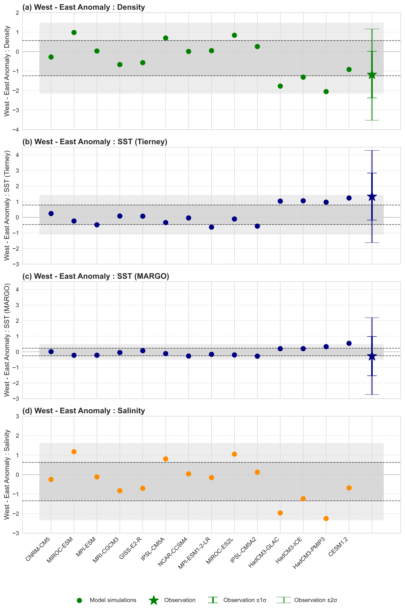
Figure 12 Model–data comparison of West–East anomalies (LGM − piControl) in the Indian Ocean. Grey shaded areas indicate model uncertainty (±1σ, light shading ±2σ), based on simulation ensembles. Stars denote reconstruction-based anomalies and are shown for comparison only. All model values are extracted at the same grid cells as the observational sites to ensure a spatially consistent comparison. Regional uncertainties are obtained by combining uncertainties from all sediment cores from each box (West and East). For each core, the uncertainty is represented by a Gaussian standard deviation derived from its reported confidence interval. We construct inverse-variance reliability weights using two components: the within-core variance (from the CI-based σ) and the between-core spatial variance (the variance of core-specific means). The regional mean is the weighted average of the core means, and its uncertainty follows the law of total variance, ensuring that both local reconstruction uncertainty and spatial variability are preserved. To obtain smooth uncertainty bands, we then generate Monte-Carlo draws from this mixture. Uncertainty on the West–East anomaly is then obtained by standard error propagation, assuming independent regional means (square root of the sum of squared standard deviations). (a) Surface density anomaly (kg m⁻³). Density reconstructions are derived from δ¹⁸O_c measurements of planktonic foraminifera and converted into density estimates using the Bayesian calibration method of Caley et al. (2026). Observational uncertainty is shown by the 68 % (dark green) and 95 % (light green) confidence intervals. (b) Sea surface temperature (SST) anomaly (°C) based on Tierney et al. (2020). Observational uncertainties are shown as 68 % (dark blue) and 95 % (blue). (c) same as (b), but using the MARGO database (MARGO Project, 2009). (d) Sea surface salinity (SSS) anomaly (g kg⁻¹).

DiNezio et al. (2018) investigated the LGM − piControl SST anomaly in this part of the Indian Ocean using the CESM1 model, revealing a West–East SST gradient in this region. Their study showed that two main mechanisms drive the observed glacial-interglacial climate changes: first, the exposure of the Sahul shelf enhances ocean-atmosphere feedbacks that alter rainfall and temperature gradients across the Indian Ocean; second, Northern Hemisphere cooling weakens monsoonal systems by reducing moisture supply, especially over the Arabian Sea. This sensitivity is also dependent on how the newly exposed continental shelf is represented in the model. Factors such as the prescribed surface roughness, vegetation type, or albedo in the now-exposed Indonesian region can significantly impact the simulated atmospheric circulation (DiNezio and Tierney, 2013; Dinezio et al., 2018). In particular, the ability of the convection scheme to respond differently to land versus ocean surfaces plays a critical role in shaping regional precipitation patterns (Chemel et al., 2014). These model design choices likely contribute to the spread of results across PMIP3 and PMIP4 model simulations and their varying skill in reproducing observed SST and surface density gradients.

Salinity biases were also assessed using LGM − PI anomalies and West–East gradients (Fig. 12d). Without direct LGM salinity reconstructions, this relies on model outputs. Inter-model spread in salinity is comparable to density and larger than SST, emphasizing the role of freshwater fluxes and hydrological processes in shaping density changes. Model simulations with the most negative salinity anomalies (MRI-CGCM3, GISS-E2-R, HadCM3-GLAC-1D, HadCM3-ICE-6G_C, HadCM3-PMIP3 and CESM1.2) best reproduce the observed west–east density gradient. Model simulations failing to produce sufficiently negative salinity anomalies often have biases in monsoon precipitation location and intensity, directly affecting surface salinity. Dinezio and Tierney (2013) showed that accurate West–East salinity gradients require correct precipitation patterns. This underscores the importance of correctly simulating the Indian Ocean hydrological cycle (including major rivers) and atmospheric circulation to reproduce salinity-driven density gradients and associated climate impacts.

In particular, DiNezio and Tierney (2013) showed that HadCM3 is the only model exhibiting statistically significant agreement with proxy-based rainfall reconstructions in the Indo-Pacific region. In our analysis, some HadCM3 simulations also perform well, particularly in reproducing the west–east density gradient (Fig. 12).

All HadCM3 simulations follow the PMIP4 protocol for implementing LGM boundary conditions. This protocol ensures that the differences between ice-sheet reconstructions are consistently applied – not only in terms of ice-sheet mask and elevation, but also land–sea distribution, bathymetry, and far-field topography. Among them, the HadCM3-ICE-6G_C simulation provides the best agreement with the observed west–east surface density gradient. This improved performance is consistent with previous results (Izumi et al., 2023), who showed that the ICE-6G_C ice-sheet configuration induces distinct atmospheric circulation responses compared to other reconstructions. These include shifts in jet structure and stationary waves, as well as differences in surface albedo forcing and sea-ice expansion. Such large-scale circulation adjustments feedback onto the Indo-Pacific climate, which likely explains the slightly more realistic simulation of the west–east density gradient in HadCM3-ICE-6G_C.

To summarize, our results confirm a strong cooling in the eastern Indian Ocean contrasted with milder cooling in the western basin, leading to a reduction of the zonal SST gradient compared to preindustrial conditions (DiNezio et al., 2018).

We also demonstrate that this zonal SST changes are associated with zonal salinity and density changes. Of the 14 model simulations, only 7 (50 %) successfully reproduce the observed West–East tropical gradient both in SST and density during the LGM, when accounting for the 68 % uncertainty range of the reconstructions. This highlights current climate model limitations, indicating that key processes are insufficiently represented or that boundary condition choices, especially ice-sheet reconstructions, could influence model–data agreement and underscores the value of palaeoclimate for improving our understanding of Indian Ocean mean state under varying boundary conditions.

This is of importance because mean state changes, as shown by Abram et al. (2020), likely enhanced interannual variability across the basin. Although previous study on IOD variability in PMIP simulations does not show a systematic relationship with changes in the mean zonal gradient across different climatic states in term of median value (Brierley et al., 2023), investigated if the simulations that perform the best to reproduce the gradient also show specific interannual variability would be interesting for future works.

5 Conclusions

The quantitative density reconstruction method based on δ¹⁸O_c, developed by Caley et al. (2026), provides a valuable dataset for evaluating climate model simulations from PMIP3 and PMIP4 in terms of LGM density changes. Instead of comparing ensemble means, our analysis evaluates each model simulation individually.

Overall and at the global scale, model simulations tend to slightly underestimate the magnitude of density anomalies compared to proxy-based reconstructions, which exhibit a mean anomaly of ∼1.6 kg m⁻³, while model simulations average around 1.1 kg m⁻³ with a range from 0.6 to 1.6 kg m⁻³. Accounting for reconstruction uncertainty improves the agreement between simulations and reconstructions, particularly by reducing discrepancies in variability. However, substantial differences between simulated and reconstructed global surface density anomaly (LGM − PI) distributions remain.

Taylor diagrams and complementary performance metrics, indicate that all simulations capture key features of the reconstructed surface densities to some extent, resulting in moderate to good overall agreement for the LGM and the PI time periods. Several simulations, including MRI-CGCM3 and IPSL-CM5A2 and the two iLOVECLIM experiments, consistently perform well across multiple global metrics. Nevertheless, this apparent global agreement masks substantial regional discrepancies revealed by the regional analyse of the Indian Ocean.

Most simulations reproduce reconstructed surface density field in the Indian Ocean reasonably well, regardless of the climatic period considered, but simulations performance is nevertheless systematically lower in the North Indian Ocean than in the South Indian Ocean. In addition, while the basin-scale density changes are reasonably reproduced, except for iLOVECLIM simulations, only 7 out of 14 remaining simulations (50 %) capture the weakened West–East density gradient. This misrepresentation of the mean state of the IOD-like could affect our understanding of past IOD variability.

Discrepancies between simulated and reconstructed surface ocean density are linked to biases in SST and salinity changes, and to insufficient representation of low-latitude precipitation reductions, which are critical for reproducing density anomalies in tropical regions.

These results emphasize that evaluating individual simulations rather than ensemble means is essential, as ensemble averaging can mask inter-model differences and region-specific biases. They also demonstrate the importance of complementary diagnostics across multiple spatial scales, from global distributions to basin-scale performance metrics and finally to tropical west–east gradients. Together, these provide a more complete assessment of model skill than any single metric alone. They also highlight the need to expand LGM density reconstructions, particularly in poorly sampled open-ocean regions, to provide stronger observational constraints on model simulations. In the future, integrating these datasets within statistical observational-constraint frameworks and data assimilation approaches could help identify model simulations that most accurately reproduce past climate states and could ultimately improve confidence in future climate projections.

Appendix A: Study basins

We first considered the major oceanic basins: The Atlantic, Indian, and Pacific Oceans, the circumpolar Southern Ocean. To better capture regional processes and analyze these regions more precisely, some of these large basins were subdivided into northern and southern parts, resulting in a total of eight ocean basins. Specifically, the North Atlantic, following the density reconstruction method of Caley et al. (2026), extends from 0 to 40° N, while the South Atlantic is restricted from 0° N to 40° S. Similarly, the North Indian Basin extends from 0° S northward, and the South Indian and Pacific Basins are restricted from 0° N to 40° S. The North Pacific is separated from the North of 40° N basin at 40° N of latitude.

The Mediterranean Sea was excluded from the analysis, as this region is particularly difficult for climate models to simulate and the limited number of proxy data points resulted in statistically insignificant regressions.

The study basins were defined using the NOAA WOA23 mask file (1° × 1° grid: https://www.ncei.noaa.gov/data/oceans/woa/WOA23/MASKS/basinmask_01.msk, last access: 1 February 2025), with modifications applied to create these eight final regions (Fig. A1).

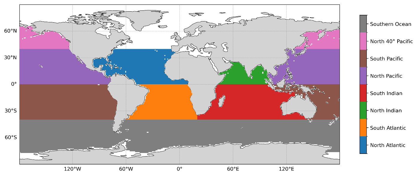
Figure A1 Map of selected basins in this study. The study basins were created from the NOAA WOA23 mask file (which has a 1° × 1° grid) (website https://www.ncei.noaa.gov/data/oceans/woa/WOA23/MASKS/basinmask_01.msk, last access: 1 February 2025) then some basins were modified, in particular to divide them into North and South. 8 basins were defined and studied: North Indian (latitudinal limit at 0° S), South Indian (latitudinal limit at 40° S), North Atlantic (between 0 and 40° N), South Atlantic (latitudinal limit at 40° S), North Pacific, South Pacific, North Pacific with latitudes > 40° N, and Southern Ocean. North Atlantic is cropped at 40° N following the Caley et al. (2026) density-reconstruction method.

Appendix B: Latitudinal profiles of surface density, SSS and SST anomalies (LGM − PI)

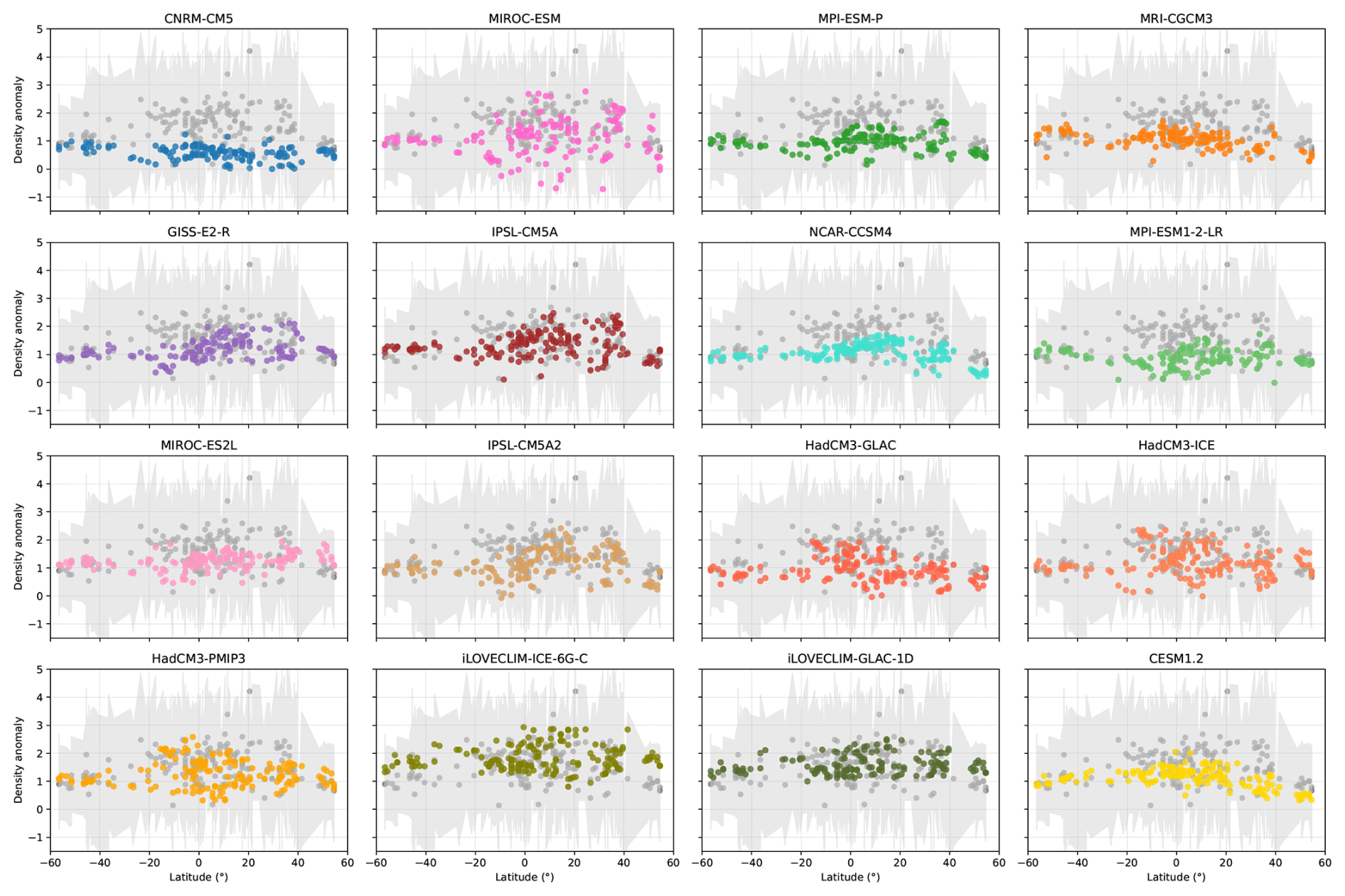
Figure B1 Density anomaly (kg m⁻³) as a function of latitude for each model simulation (colored dots), compared with observational data (grey dots) and the 95 % confidence interval (grey shading). Model outliers, identified using the interquartile range (IQR) method (values outside 1.5 × IQR), were excluded to minimize the influence of extreme values and highlight robust spatial patters. This filtering enhances the main latitudinal structure and modelled density anomalies while preserving all available latitude sampling points.

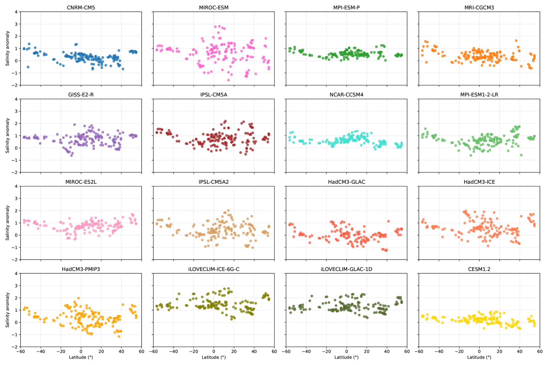
Figure B2 Zonal distribution of salinity anomalies (LGM − PI) simulated by each model (colored dots). Model outliers, identified using the interquartile range (IQR) method (values outside 1.5 × IQR), were excluded to minimize the influence of extreme values and highlight consistent spatial patterns. This filtering emphasizes the latitudinal structure of simulated salinity anomalies across models while preserving all available sampling points.

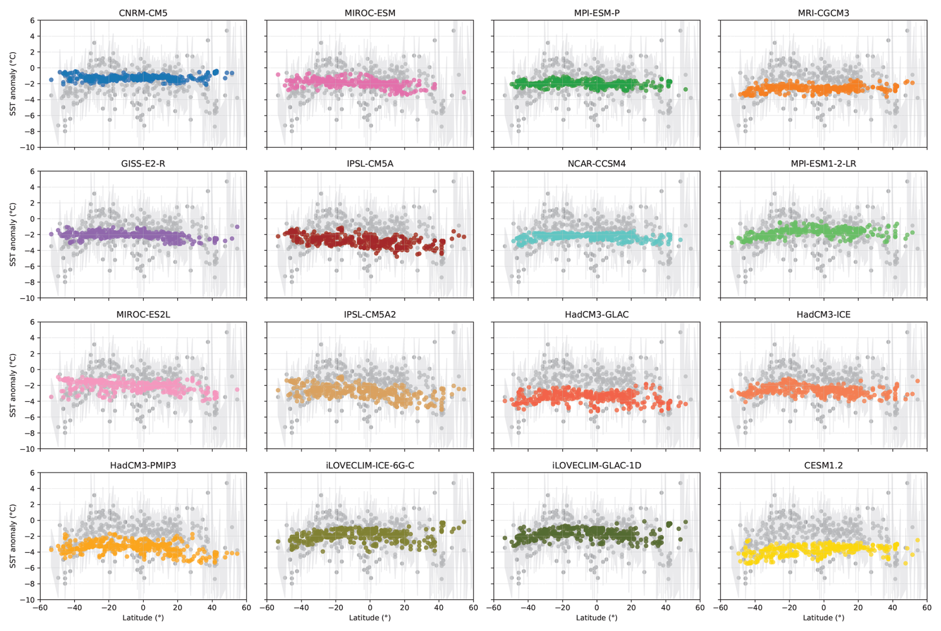
Figure B3 Zonal distribution of SST anomalies (LGM − PI) from the MARGO (MARGO project, 2009) reconstruction (grey dots) and ±1σ uncertainties (grey shading), compared with model simulations (colored dots). Model outliers, identified using the interquartile range (IQR) method (values outside 1.5 × IQR), were excluded to minimize the impact of extreme values and highlight robust latitudinal patterns. This filtering enhances the readability of the large-scale SST anomaly structure while preserving all available latitude points.

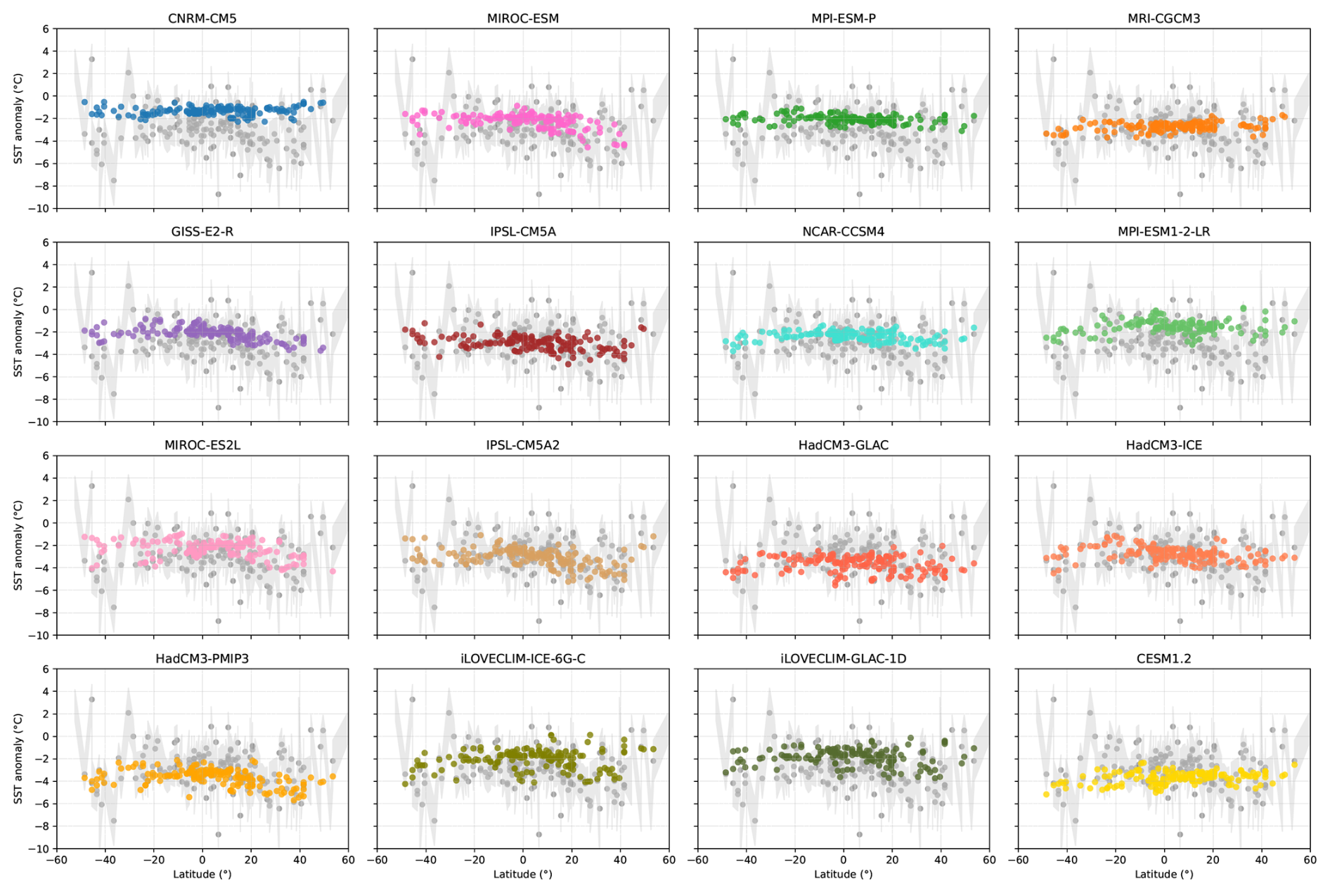
Figure B4 Zonal distribution of SST anomalies (LGM − PI) from Tierney et al. (2020) reconstruction (grey dots) and ±1σ uncertainties (grey shading), compared with model simulations (colored dots). Model outliers, identified using the interquartile range (IQR) method (values outside 1.5 × IQR), were excluded to minimize the impact of extreme values and highlight consistent spatial patterns. This filtering clarifies the latitudinal structure of simulated SST anomalies while preserving all available observation–model comparison points.

Appendix C: Comparison of global distribution of surface density anomalies

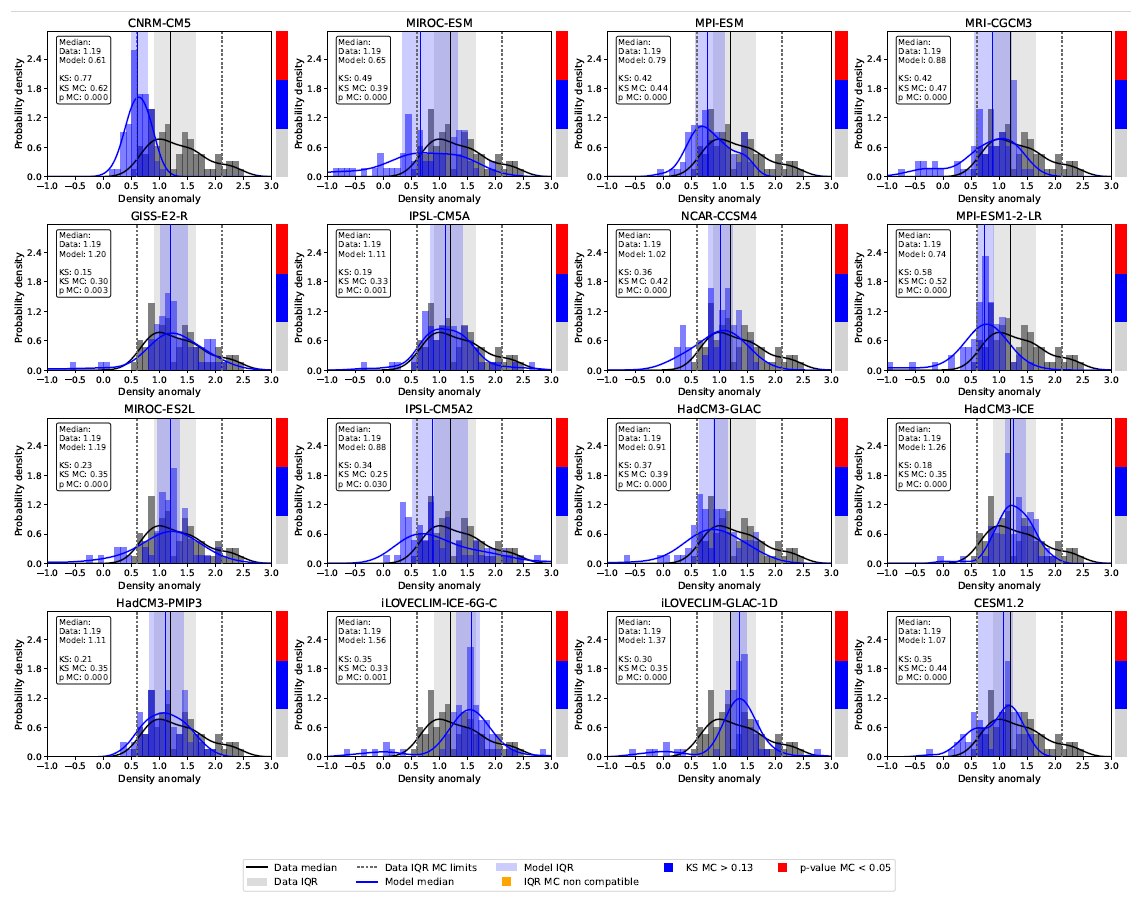
Figure C1 Distribution histograms of surface density anomalies (LGM − PI, kg m⁻³) at the global scale. Density reconstructions are shown in black, model simulations in blue. Kernel Density Estimates (KDEs) illustrate the central tendency and overall shape of the distributions. Vertical lines indicate the median of each distribution, and shaded envelopes represent the interquartile ranges (IQRs), providing a measure of data spread that is independent of extreme values. Grey dotted lines indicate the limits of the Monte Carlo propagated reconstruction IQR obtained after accounting for the 95 % confidence intervals associated with the density reconstructions. The histograms display the frequency of values, complementing the KDEs and IQRs to give an integrated view of distribution characteristics. Reconstructions uncertainties are explicitly propagated through the Monte Carlo procedure. Colored indicators on the right side of each panel summarize the outcomes of the three comparison metrics. A red flag indicates a Monte Carlo-derived two-sample KS test with p< 0.05, a blue flag indicates a Monte Carlo-derived KS statistic exceeding the global critical threshold (KS > 0.13), and an orange flag indicates non-overlapping Monte Carlo propagated IQRs between reconstructed and simulated distributions.

Appendix D: Global Evaluation of Surface Density: Models vs. Reconstructions (PI and LGM)

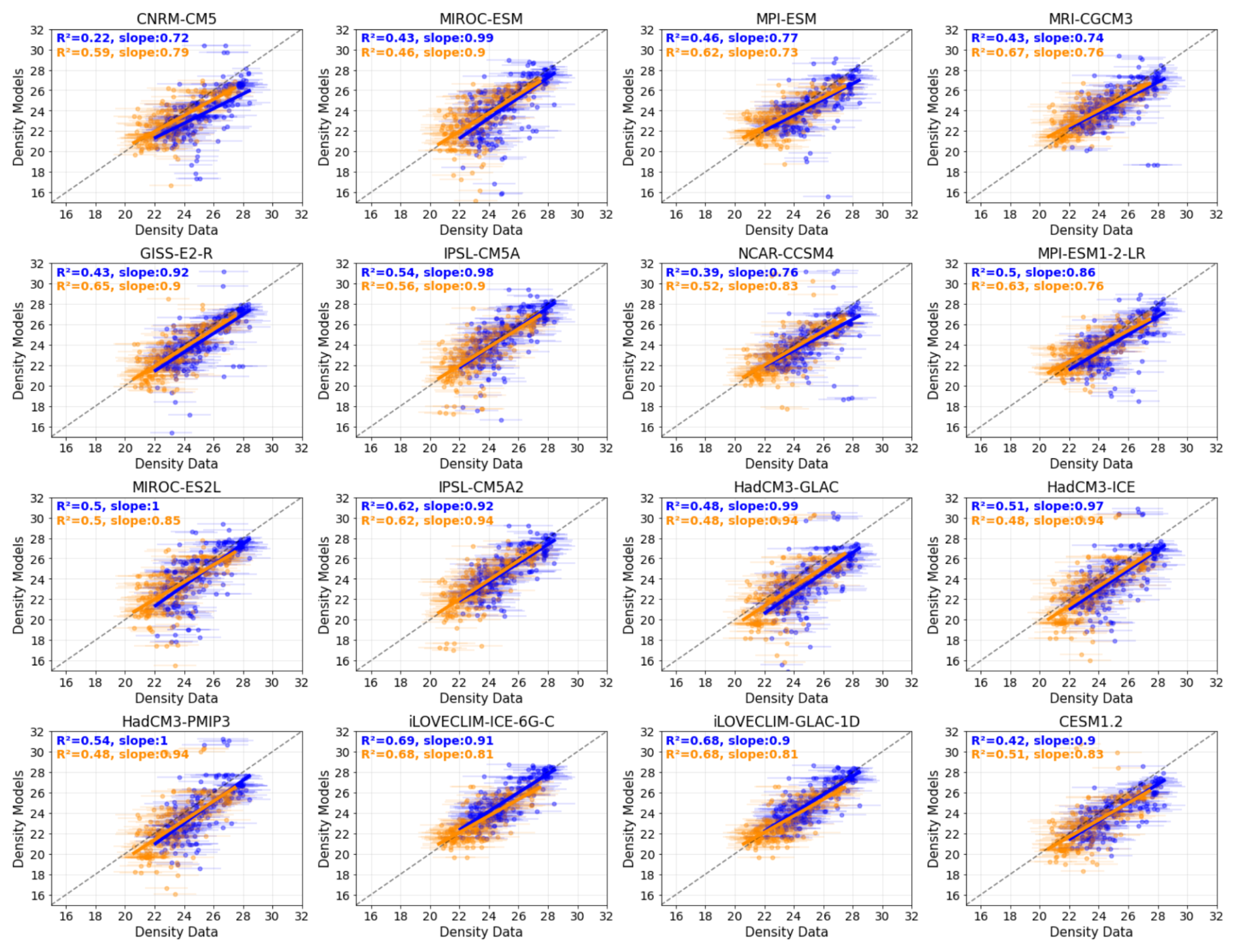
Figure D1 Linear regressions between absolute surface density (kg m⁻³) from proxy-based reconstructions (x-axis) and model simulations (y-axis), aggregated at the global scale (across all selected basins). Results are shown for the LGM period (blue) and the piControl period (orange). Error bars on the x-axis represent the 95 % confidence intervals of the reconstructed values. The slope and R² values correspond to standard linear regressions, accounting for uncertainties on the x-axis (the Monte Carlo method was applied here). All regressions shown are statistically significant (p< 0.05).

Appendix E: Focus on the Indian Ocean

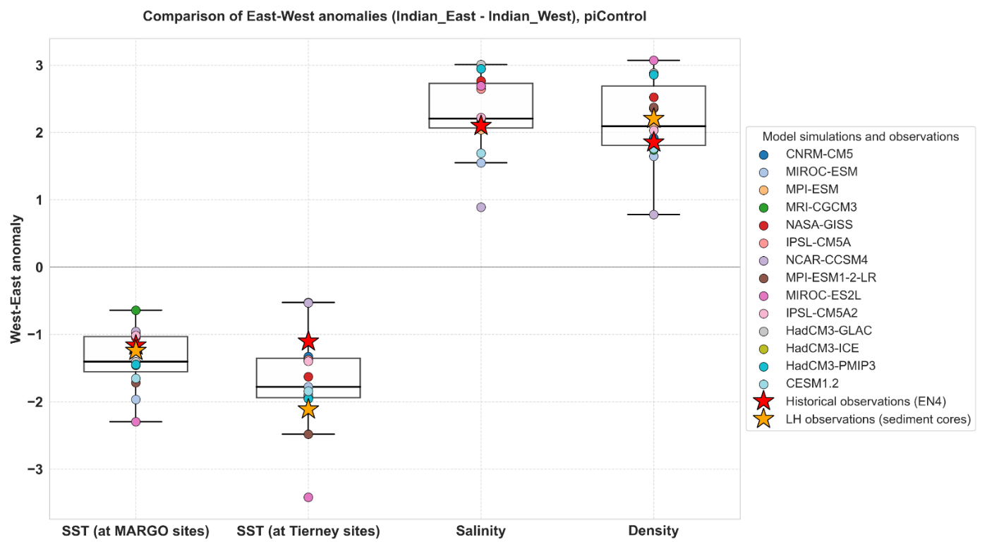
Figure E1 Boxplots showing West–East anomalies (Indian_East – Indian_West) in Sea Surface Temperature (°C), (from the MARGO and Tierney datasets, separately), Sea Surface Salinity (g kg⁻¹), and sea surface density (kg m⁻³) during the pre-industrial period. The boxplots represent the distribution of anomalies from climate model simulations only. Each colored dot corresponds to the anomaly from an individual model simulation. Red stars indicate observed values from the EN4 dataset (Good et al., 2013), averaged over the period 1900–1999 to provide a historical reference. Orange stars indicate reconstructions from databases (PI from WOA18 for MARGO (MARGO project, 2009), LH for Tierney et al. (2020) and LH (Late Holocene) for density; Caley et al., 2026). The “Indian West” box is defined as 50–70° E, 12° S–12° N, corresponding to the tropical western Indian Ocean. The “Indian East” box is defined as 90–110° E, 10° S–2° N, corresponding to the tropical south-eastern Indian Ocean.