Limited atmospheric iron availability increase during the Younger Dryas in the Northern Hemisphere

Iron (Fe) availability modulates phytoplankton blooms in High-Nutrient Low-Chlorophyll (HNLC) regions, i.e., ocean areas characterized by an abundance of major nutrients but low marine productivity. Fe can be delivered to the oceans through atmospheric dust deposition, making ice cores unique archives for reconstructing past changes in aeolian Fe deposition. However, while it is known that during dustier periods atmospheric Fe depositions increased, uncertainties remain regarding the fraction of Fe actually available to phytoplankton. Here, we present evidence from the EGRIP ice core (Greenland) during the Pleistocene-Holocene transition (10.3–13.0 ka), which provides insights into atmospheric aerosol deposition over the Fe-limited North Pacific Ocean. Results show that, in contrast to the 17-fold enhancement in total Fe determined by Inductively Coupled Plasma Mass Spectrometry, the iron fraction more likely available for phytoplankton (i.e., labile iron) increased only modestly (+29 %) during the Younger Dryas compared to the Early Holocene, likely due to prevailing alkaline aerosol conditions reducing its solubility. This finding supports the hypothesis that factors other than atmospheric Fe deposition (e.g., stronger water stratification, sea-ice extent, volcanic eruptions, iron remobilization from sediments), played a more relevant role in regulating marine net primary productivity in the HNLC North Pacific Ocean over the last glacial transition.

1 Introduction

Iron (Fe) plays a crucial role in oceanic biogeochemistry, serving as a co-factor in enzymes involved in photosynthesis and atmospheric nitrogen fixation (Mills et al., 2004). Its bioavailability and abundance in the ocean can limit net primary productivity (NPP), even when other major nutrients such as nitrate and phosphate are abundantly present. Regions where this occurs are known as High-Nutrient Low-Chlorophyll (HNLC) areas, which account for up to 20 % of the world's ocean surface and include the Southern Ocean, the Equatorial Pacific, and the North Pacific Ocean (Duggen et al., 2010). In these regions, aeolian Fe deposition can act as a fertilizer, triggering and modulating NPP and thus influencing CO₂ exchanges between the atmosphere and the ocean (Martin and Fitzwater, 1988).

The link between iron fertilization and the biological carbon pump was first explored by oceanographer John Martin. His hypothesis, known as the iron hypothesis, suggests that higher aeolian iron fluxes deposited on HNLC ocean surfaces during colder and dustier periods would have stimulated NPP, enhancing the drawdown of atmospheric CO₂ into the oceans and explaining the 80–100 ppm lower CO₂ concentrations observed during glacial periods compared to warmer, less dusty, interglacial periods (Martin et al., 1990). Modelling and observational evidence confirmed that Martin's intuition was correct (Boyd et al., 2007), although the impact of Fe fertilization has since been substantially downscaled (Stoll, 2020; Saini et al., 2023). Other processes, such as stronger oceanic stratification and deep-water ventilation during glacial times, played a more important role (Francois et al., 1997; Lambert et al., 2021; Weber et al., 2022; Schmitt et al., 2012; Bauska et al., 2016). Nevertheless, millennial-scale Earth System Model simulations estimated that up to 20 ppm of the glacial CO₂ decline can be still attributed to a more globally efficient biological carbon pump enhanced by atmospheric iron deposition during the last glacial maximum (Lambert et al., 2015).

Besides aeolian mineral dust, volcanic ash represents an additional source of iron to surface waters (Langmann et al., 2010). Although acting on shorter time scales (i.e., months to maximum a few years), it was first hypothesized (Spirakis, 1991), and subsequently demonstrated, that iron contained in volcanic ash can stimulate phytoplankton blooms in HNLC ocean areas (Langmann et al., 2010; Frogner et al., 2001). Observed decreases in atmospheric CO₂ following major eruptions such Agung (1963) have been interpreted as evidence of the fertilizing effect of ash-derived Fe on ocean productivity (Watson, 1997). Other sources of bioavailable iron include biomass burning, and, on more recent time scales, anthropogenic emissions (Matsui et al., 2018).

The response of HNLC regions to Fe fertilization during glacial periods varied regionally. In the Southern Ocean, enhanced atmospheric Fe fluxes induced an increase in NPP in the Subantarctic Zone, as inferred from sea-sediment records (Martínez-García et al., 2014; Jaccard et al., 2013), while the net effect over the whole Southern Ocean was much smaller (Fischer et al., 2025). In the North Pacific Ocean, NPP showed no significant response to enhanced atmospheric Fe fluxes over the last 800 ka (Kienast et al., 2004; Burgay et al., 2021a). While limited nutrient upwelling, sea-ice extent and iron remobilization from sediments have been acknowledged as key drivers regulating NPP in this region (Kienast et al., 2004; Praetorius et al., 2015), a crucial question remains unanswered: to what extent was atmospheric aerosol iron actually available to phytoplankton?

Given that iron is a key component of mineral dust, its quantification in ice cores represents a valuable approach for assessing changes in atmospheric iron concentrations and solubility during past climatic transitions. To quantify iron in ice cores, different methodologies exist, each of them targeting a specific operationally defined Fe fraction. Total dissolvable iron (TDFe) is defined as iron determined in discrete samples by Inductively Coupled Plasma Mass Spectrometry (ICP-MS) after at least four weeks of acid (2 % HNO₃) digestion at pH =1 (Burgay et al., 2021a; Edwards and Sedwick, 2001). However, TDFe overestimates the bioavailable Fe fraction as long acidic digestions allow for more complete dissolution of acid-labile Fe (Vallelonga et al., 2013; Edwards et al., 2006). ICP-MS has been also used to continuously quantify Fe after shorter (few seconds) acidification times (Fe_ICP). Fe_ICP captures most of the atmospheric Fe pool, but, as TDFe also does, excludes the fraction structurally bound with refractory silicates, which would require strong acid digestion for complete dissolution (Gaspari et al., 2006). Fe_ICP may overestimate the dissolved fraction when a non-negligible amount of undissolved mineral particles is present, such as during dusty periods (Erhardt et al., 2019). The form more readily accessible to phytoplankton (dissolved Fe, DFe) can be quantified using discrete sampling approaches. These methods typically involve filtering melted ice samples through 0.2 or 0.45 µm filters, followed, sometimes, by acidification with HNO₃ (Du et al., 2019) or HCl (Winton et al., 2016). Representative seawater soluble Fe analyses have also been performed by sublimating ice under vacuum, then leaching the residual dust particles with seawater (Conway et al., 2015). Continuous measurements of iron involve online acidification of the meltwater stream from a Continuous Flow Analysis (CFA) system, followed by absorption detection (Burgay et al., 2019; Hiscock et al., 2013). The mild acidification step at pH ≈ 1.6 with HCl releases iron bound from both colloidal forms and iron-binding ligands (Lohan et al., 2006), as well as it breaks down Fe-hydroxides and Fe-complexes into dissolved free Fe (Hiscock et al., 2013). This iron corresponds to an easily leachable and labile fraction, which, in Holocene samples, accounts for 20 %–30 % of Fe_ICP (Erhardt et al., 2019). Due to methodological differences, however, this fraction cannot be directly compared with the standard operational definition of DFe discussed above and used in many oceanographic studies by the GEOTRACES community (http://www.geotraces.org, last access: 2 September 2026). To make this distinction, we refer to this fraction as labile iron (LFe). We interpret LFe as a proxy for the potentially bioavailable iron fraction (Hiscock et al., 2013), i.e., the iron fraction that is most prone to become available for complexation by phytoplankton siderophores once deposited in seawater (Yoshida et al., 2002). From this perspective, LFe should be interpreted as an upper bound on the pool of potentially bioavailable iron, rather than a direct measure of iron available for phytoplankton uptake.

Here, we present the first continuous Fe_ICP and LFe measurements during the Pleistocene-Holocene transition (10.3–13.0 ka) from the EGRIP ice core (Greenland), to investigate changes in iron concentrations during the Younger Dryas (YD), a high-dust climate cold event, and the subsequent Preboreal transition into the warm, low-dust Holocene.

2 Material and methods

2.1 EGRIP ice core

The East Greenland Ice-core Project (EGRIP) retrieved a 2665-meter-long ice core to investigate how ice streams may contribute to future sea-level change. The EGRIP drill camp was located within the North-East Greenland Ice Stream (NEGIS), approximately 360 km NNE from the Greenland Summit (red star in Fig. 1, 2708 m a.s.l., 75.63° N, 36.00° W) (Erhardt et al., 2023). The NEGIS drains ice from the interior of the ice sheet towards marine-terminating outlet glaciers in North-East Greenland, at modern surface velocities of 55 m a⁻¹ (Hvidberg et al., 2020). The EGRIP ice was therefore likely deposited ≈ 180 km upstream towards the ice divide at the time of deposition (10.3–13.0 ka), as compared to present day (Gerber et al., 2021), although recent evidence showed that the shear margins of NEGIS may have only developed 2000 years ago (Jansen et al., 2024). The core was dated using published chronology (GICC05 transfer from NGRIP on volcanic matching), with a maximum counting error (MCE) between 89 (10.3 ka) and 141 (13.0 ka) years (Mojtabavi et al., 2019).

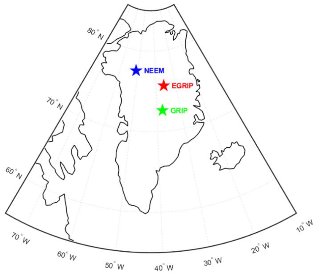
Figure 1 Map of Greenland and location of three different Greenland ice-core locations discussed in the main text: EGRIP (red star), NEEM (blue star) and GRIP (green star).

LFe and Fe_ICP data from EGRIP are compared with other Greenland ice-core iron records, including NEEM (77.45° N, 51,06° W, blue star in Fig. 1; Burgay et al., 2021a) and GRIP (72.35° N, 37.38° W; green star in Fig. 1; Hiscock et al., 2013). NEEM and GRIP are both located on the Greenland plateau at 2540 and 3230 m a.s.l., respectively, with modern accumulation rates of 22 and 23 cm ice equivalent per year (Andersen et al., 2006; Schüpbach et al., 2018).

To provide a comprehensive and inter-hemispherical comparison, the Fe records from Greenland were compared with an ice core from Antarctica (Epica Dome C, EDC96, 75°06^′ S; 123°21^′ E) (Traversi et al., 2004). EDC96 is located in the Antarctic Plateau at 3233 m a.s.l., with a modern accumulation rate of 2.9 cm ice equivalent per year (Udisti et al., 2004).

2.2 The Bern Continuous Flow Analysis system (Bern-CFA)

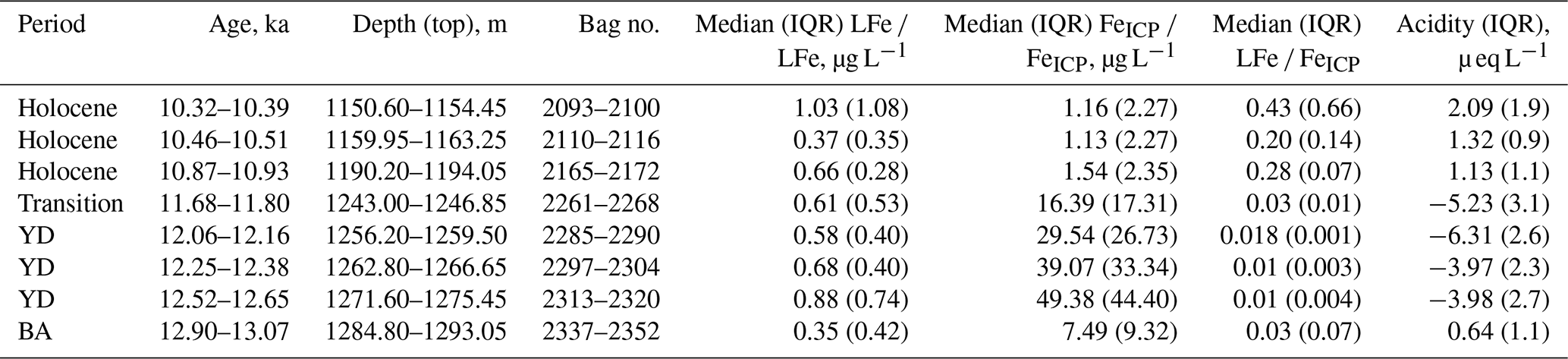
The Bern Continuous Flow Analysis (Bern-CFA) is used to analyze elements and major ions in polar ice cores at a high temporal resolution (≈ 1 cm-depth resolution). Ice samples were cut with a section of 36 × 36 × 550 mm, known as a “bag”. The ice is melted at a speed of 2.8 cm min⁻¹ along the core axis on a gold melt head inside a −20 °C cold room. To remove contamination of the ice due to handling or drilling fluid, only the meltwater from the innermost 26 × 26 mm of the ice is used for analysis. The resulting meltwater is directed toward two sections for analyses: a wet-chemistry and a single particle ICP-TOF-MS (spICP-MS) section. The wet-chemistry line detects soluble Ca²⁺, NH${}_{\mathrm{4}}^{+}$, NO${}_{\mathrm{3}}^{-}$, concentration and size distribution of insoluble particles, conductivity, black carbon, acidity, and LFe (Kaufmann et al., 2008; Burgay et al., 2019; Erhardt et al., 2023; Kjær et al., 2016). The spICP-MS line provides continuous trace element profiles and allows single particle characterization in selected intervals (Erhardt et al., 2019). Here, we present a continuous quantification of Fe_ICP, acidity, dust and conductivity between 10.3 and 13.0 ka. Eight selected periods during the Holocene (n=23 bags), Younger Dryas (YD, n=30) and Bølling-Allerød (BA, n=16) have been analyzed also for LFe (Table 1).

Table 1 Selected period (n=8) over the Holocene, Younger Dryas (YD) and Bølling-Allerød (BA) of median LFe, Fe_ICP, LFe $/$ Fe_ICP ratio and acidity based on continuous sampling. Median and interquartile range (IQR) are reported. Median LFe $/$ Fe_ICP ratio is calculated as a bag mean. Volcanic eruptions are included.

2.2.1 LFe and Fe_ICP continuous quantification

LFe concentrations are quantified using the continuous absorption method described in Burgay et al. (2019) at a resolution of 1 cm. The ice-core meltwater flow for LFe analysis was 0.9 mL min⁻¹. Raw LFe transmittance values (λ=514 nm) were acquired every second using the OceanView software (Ocean Optics) and later converted into absorption values. Absorbance values were converted into concentration units (µg L⁻¹) using the Beer-Lambert law, with an optical path length set to 1 cm (Fig. S1 in the Supplement). Calibration curves were performed before and after each analytical run, to account for any sensitivity changes. Calibration standards were prepared by diluting a certified Fe stock solution at 1000 mg L⁻¹ (Fe(NO₃)₃, Certipur^®, Merck) to 0.5–10 µg L⁻¹, based on expected concentrations throughout the record (Table S1). To monitor and correct for blank drifts, ultrapure water samples were analyzed at the beginning and end of each sample run. The LFe limit of detection (LoD), calculated as three times the standard deviation of 10 Ultrapure Water (UPW) blanks, was determined to be 0.08 µg L⁻¹. Accuracy, evaluated using a 0.5 ng g⁻¹ standard solution, was 96 %. Reproducibility, evaluated by performing five replicate measurements of a 0.5 ng g⁻¹ standard solution, was 8 % RSD. In correspondence with two specific volcanic eruptions (12.91 and 13.03 ka BP), the spectrophotometric detector saturated, preventing a reliable quantification of LFe for these volcanic horizons.

Fe_ICP was quantified using spICP-MS equipped with a collision cell (Q-Cell) that removes isobaric interferences (e.g., ⁴⁰Ar¹⁶O⁺), enabling the determination of the most abundant Fe isotope (⁵⁶Fe), and a time-of-flight mass spectrometer. Meltwater flow rate for Fe_ICP was 1.0 mL min⁻¹. The LoD, calculated as three times the standard error of intercept from the calibration curve, was quantified to be 0.12 µg L⁻¹. Resolution is 1 cm. Regular calibrations were performed after each run by diluting certified Fe standard solution at 1000 mg L⁻¹ (Ventures IV-STOCK-1643 Multielemental standard) to 0.2–1000 µg L⁻¹, based on the expected concentrations throughout the record. Further details in Erhardt et al., (2019).

2.2.2 Acidity, conductivity and particulate dust measurements

Acidity was determined using a continuous absorption method (Kjær et al., 2016) based on two dyes (bromophenol blue and chlorophenol red), which change color, and thus absorption values, depending on pH. Bromophenol blue changes from yellow at pH 3.0 to purple at pH 4.6, while chlorophenol red shifts from yellow at pH 4.8 to violet at pH 6.7. Standard solutions were prepared by diluting 1.0 M HCl and 1.0 NaOH stock solutions. For the Holocene period, standards were prepared at −2.5, 2.5 and 4 µ eq L⁻¹. For the YD and BA, standards were prepared at −4.9, −2.5 and 2.5 µ eq L⁻¹. Calibration curves were performed before and after each analytical run, to account for any sensitivity change. Acidity values should be interpreted qualitatively, as the calibration standards are influenced by CO₂ dissolution from laboratory air, whereas the CFA meltwater stream is likely not. For the purpose of this work, negative values represent standards/samples that are more alkaline than pH =5.4 (UPW).

In addition to acidity, electrolytic meltwater conductivity was measured using a conductivity cell (3082 with micro flow cell 829, Amber Science), while a laser attenuation particle counter and sizer (Abakus with LDS 23/25 bs sensor, Klotz) was used for determining insoluble particle concentrations (Kaufmann et al., 2008; Erhardt et al., 2023; Simonsen et al., 2018). The conductivity is sensitive to changes in ice acidity, i.e., variations in H⁺ concentration, with higher values corresponding to higher acidity. Coldest periods, which have an enhanced concentration of alkaline dust, present a significantly reduced conductivity compared to interglacial periods (Taylor et al., 1993). Insoluble particle concentrations are measured using an Abakus laser sensor, which determines the optical extinction cross section of particles in the 1–15 µm size range (Simonsen et al., 2018).

2.2.3 Raw data treatment and data alignment with the CFA data

Once calibrated, LFe data was aligned with conductivity data provided by the Bern-CFA (SM – Sect. 1) as previous studies have shown a correlation between these parameters in Holocene samples (Burgay et al., 2019). Cross-correlation techniques were applied as they are commonly used to compare time series and identify the degree of linear similarity between datasets at varying time lags. To measure the time delays between two time series of irregularly sampled data and align them, the Interpolated Cross-Correlation Function (ICCF) was employed (Gaskell and Sparke, 1986). For each sample run, the ICCF was calculated at a sequence of time lags, and the lag corresponding to the maximum correlation value was selected as the optimal alignment point. This process was repeated across the different sample runs to align LFe with conductivity (SM – Sect. 2). Computation of ICCF were performed with the R package sour freely available at the GitHub repository (Edelson et al., 2017; R Core Team, 2025). Cross-correlations between LFe and conductivity ranged between 0.51 and 0.92.

3 Results and Discussion

During the Pleistocene-Holocene transition, the ice chemistry has changed significantly. As a consequence of the sharp temperature decrease in the Northern Hemisphere during the YD, the hydrological cycle was reduced and the atmosphere became dustier, as extensively demonstrated by the higher dust, Ca²⁺(i.e., a commonly used ice-core proxy for mineral dust (Ruth et al., 2008)), and TDFe concentration compared to the Holocene (Burgay et al., 2021a; Schüpbach et al., 2018). During the YD, dust deposited in continental Greenland was sourced from the Asian (Gobi and Taklamakan) and the Saharan deserts (Újvári et al., 2022), with the latter contributing with an average of 49 % (12 %–73 %) (Han et al., 2018). Thus, a significant fraction of dust deposited in Greenland at that time was transported across the North Pacific Ocean before reaching Greenland, indicating that EGRIP, and other Greenland ice cores, are documenting changes of dust (and iron) deposition over the HNLC North Pacific Ocean, enabling the link between Fe ice-core records with NPP sea-sediment records (Serno et al., 2015). The representativeness of the LFe ice-core record presented here with the amount of labile iron deposited in the North Pacific Ocean is supported by the comparison of dust fluxes from sediment core SO202-7-6 (Subarctic North Pacific Ocean), with the high-resolution dust flux record from the NGRIP ice core (Serno et al., 2015). The comparison shows a good coherence in temporal dust deposition changes in Greenland and the Subarctic North Pacific and therefore that atmospheric deposition of iron-bearing particles deposited in Greenland are representative of what has been deposited over the Subarctic North Pacific Ocean. What differs between marine sediments and ice cores is the amplitude of the observed changes, with NGRIP showing a much larger variability in dust fluxes. This enhanced amplitude has been attributed to more efficient dust transport to Greenland and extended atmospheric residence time, driven by climate-related shifts in atmospheric circulation and wet deposition en route. While concentration and flux values from Greenland ice cores are not directly representative of the absolute amount of iron deposited in the Subarctic North Pacific Ocean, they still provide a robust record of relative changes in atmospheric dust (and iron) input in this HNLC region.

3.1 Fe_ICP record

A 17-fold increase in the median Fe_ICP concentration from the Early Holocene (1.76 µg L⁻¹, IQR =3.00 µg L⁻¹) to the YD (30.16 µg L⁻¹, IQR =30.94 µg L⁻¹) period was observed at EGRIP (Fig. 2). Unfortunately, no other Fe_ICP records exist for Greenland ice cores, making direct comparisons with other locations difficult. Nevertheless, we can compare the Fe_ICP record with the NEEM TDFe record (Burgay et al., 2021a), which was based on discrete sample that were subjected to prolonged (1 month) acidification at pH =1, before ICP-MS analysis. Notwithstanding the different methodological approaches, temporal resolution of the records, and the distinct accumulation rates between the two sites (22 vs. 11 cm ice equivalent per year at NEEM and EGRIP, respectively) (Schüpbach et al., 2018; Mojtabavi et al., 2019), median concentrations are the same within a factor of 2 for both the Holocene (2.60 µg L⁻¹, IQR =2.03 µg L⁻¹, at NEEM), and the YD (17.65 µg L⁻¹, IQR =9.9 µg L⁻¹, at NEEM), suggesting overall spatially homogeneous deposition patterns and trends across the Greenland plateau on millennial time scales.

Figure 2 (a) EGRIP δ¹⁸O profile (Vaughn et al., 2022). (b) Continuous Fe_ICP profile. (c) Continuous dust profile. (d) Acidity changes. Negative µ eq L⁻¹ values correspond to alkaline conditions. Thick solid lines are 10-year moving averages. Data gaps for dust and acidity are caused by incorrect data acquisition during the corresponding runs.

Despite the relatively high Fe_ICP concentrations observed over Greenland during the YD, and the concurrent rise in dust fluxes inferred from sediment records in the North Pacific Ocean, NPP was at low levels. Marine sediments from the North Pacific Ocean show higher NPP during the warmer and less dusty BA and Early Holocene periods (Fig. S2) (Praetorius et al., 2015; Méheust et al., 2018; Davies et al., 2011). While these observations downscale the relevance of atmospheric Fe deposition, a continuous quantification of LFe is required to assess its potential availability to phytoplankton.

3.2 LFe record and implications for marine productivity

To understand whether higher Fe_ICP concentrations were mirrored by a similar increase in LFe during the YD compared to the Holocene, and to investigate further the effects of atmospheric iron fertilization in the HNLC North Pacific Ocean, we analyzed LFe from eight different periods (Table 1). Our continuous LFe records differ from DFe measurements commonly used in oceanographic studies (Achterberg et al., 2001) and other ice-core investigations (Winton et al., 2022; Du et al., 2019), which involve filtration with 0.2 or 0.45 µm filters followed by analysis using ICP-MS. These methods are incompatible with continuous measurements due to the filtering step, which would introduce in the CFA system back-pressure issues. However, studies have shown that particulate iron (>0.45 µm) can also contribute to phytoplankton growth (Kanna et al., 2020; Visser et al., 2003), suggesting that LFe as defined in this work, i.e., the leachable fraction after acidification at pH ≈ 1.6, can be still considered as representative of the iron fraction more easily available to marine phytoplankton (Hiscock et al., 2013), although direct assessments on its true bioavailability have not yet been performed. LFe and Fe_ICP show a good alignment and seasonality with dust (Fig. S3). In Greenland, dust follows seasonal patterns due to the position of the polar front, which enables a more efficient transport of dust from lower latitudes in spring (Steffensen, 1988). Differences in the peak shape or some slight misalignments are explained by the different methods used, with LFe showing a stronger memory effect than Fe_ICP due to longer mixing coils (>2 m). In the main text, we report only one of the eight periods analyzed for LFe as an illustrative example (Fig. 3). The other periods are presented in SM – Sect. 3, together with the corresponding Fe_ICP, conductivity, acidity and LFe $/$ Fe_ICP ratio records.

Figure 3 (a) Fe_ICP (black line) and LFe (blue line) during the Pleistocene-Holocene transition (11.68–11.82 ka BP). (b) Conductivity (ECM, black line) and acidity (red line). (c) LFe $/$ Fe_ICP bag mean.

LFe median concentrations calculated over the eight investigated sections (Table 1) were at their lowest during the BA (0.35 µg L⁻¹, IQR =0.42 µg L⁻¹), while increasing by a factor of 2 during the YD (0.68 µg L⁻¹, IQR =0.53 µg L⁻¹). Values during the Early Holocene were comparable to those observed during the YD (0.62 µg L⁻¹, IQR =0.58 µg L⁻¹), contributing 20 %–40 % to Fe_ICP, consistently to what was previously observed from other polar ice cores during the Holocene (Erhardt et al., 2019; Traversi et al., 2004). To compare the concentration distributions and to better investigate differences in the aeolian LFe contributions between the Early Holocene and the YD, 10 volcanic eruptions were excluded as they are known to increase LFe (Burgay et al., 2019). The volcanic events were identified based on their documented occurrence (Lin et al., 2022) and observed acidity, LFe and conductivity increases (Table S2). Then, a two-sided Wilcoxon rank sum test was applied to compare only the aeolian LFe Early Holocene and YD distributions. The test showed that the distributions during the Early Holocene and the YD (n=7010 and, n=14 294 datapoints respectively) were significantly different (p-value $<{\mathrm{10}}^{-\mathrm{10}}$), with more frequent occurrences of higher LFe concentrations in the YD (median =0.66 µg L⁻¹) than in the Early Holocene (median =0.51 µg L⁻¹) (Fig.  4a, b). Although the increase in LFe median concentration between the Holocene and the YD is significant (+29 %, when excluding volcanic eruptions), it is not comparable with the one observed for Fe_ICP (17-fold), suggesting that the stronger dust contribution during the YD was not mirrored by a similar LFe enhancement. Consequently, the LFe contribution to Fe_ICP decreased from an average (median) of 40 % (30 %) during the Holocene to an average (median) of 2 % (2 %) during the YD. LFe contribution slightly increased during the BA to 7 % (3 %).

Figure 4 (a) Boxplot for LFe during the Early Holocene (Holo), Younger Dyras (YD) and Bølling-Allerød (BA), when excluding volcanic eruptions. (b) Probability density distribution for LFe during Holo (blue bars), YD (red bars) and BA (green bars). Dashed vertical lines refer to LFe median concentrations (blue, LFe – Holo, 0.51 µg L⁻¹; red, LFe – YD, 0.66 µg L⁻¹; green, LFe –BA, 0.30). (c) Boxplot for acidity during Holo, YD and BA, when excluding volcanic eruptions. (d) Probability density distribution for acidity during Holo (blue bars), YD (red bars) and BA (green). Dashed vertical lines refer to acidity median values (blue, acidity – Holo, 1.06 µ eq L⁻¹; red, acidity – YD, −4.93 µ eq L⁻¹; green, acidity – BA, −0.24 µ eq L⁻¹).

These findings are compared with two other available LFe studies that applied the same methodology used in this study: one from Greenland (GRIP) (Hiscock et al., 2013), and one from Antarctica (EDC96) (Traversi et al., 2004) (Table 2). At GRIP, authors investigated LFe from a 113.4 cm-long section from the Holocene referring to the periods 4.51 (52.8 cm), 6.55 (24.9 cm), and 7.61 ka (35.7 cm), and from a 109.8 cm-long core from the Glacial (28.8 ka). They report median LFe concentrations ranging from 0.14 µg L⁻¹, during the Holocene, to 0.42 µg L⁻¹ during the Glacial. The exact values differ from the ones obtained in this study because of the limited number of ice sections analyzed and different periods investigated at GRIP. While the orders of magnitude were comparable, a stronger increase in LFe is observed in GRIP between the Holocene and the Glacial (up to 3-times) than in EGRIP between the Holocene and the YD (+29 %). Overall, both the GRIP and EGRIP LFe records show only a limited increase during the coldest periods with respect to the Holocene, especially when compared with the 17-fold rise in Fe_ICP concentrations at EGRIP between the Holocene and the YD (this study) and the 15-fold increase in TDFe at NEEM between the Holocene and the last Glacial average (Burgay et al., 2021a). Although atmospheric Fe deposition increased during the YD, the amount of Fe more easily accessible to phytoplankton was much smaller.

LFe concentration values from Greenland records contrast with the only LFe record from Antarctica. During the Antarctic Cold Reversal (ACR, 11.6–14.2 ka), LFe contributed as much as 64 % of the Fe content as determined by ICP-MS (Traversi et al., 2004). In general, during cold periods (i.e., ACR and Glacial), LFe concentrations were up to 12 times (1.0 µg L⁻¹) higher than Holocene values (0.08 µg L⁻¹). Similar findings were reported from the EPICA Dome C ice core, where a tenfold increase in soluble Fe deposition fluxes during the last glacial period compared to modern values was observed (Conway et al., 2015).

There can be different players influencing Fe solubility in atmospheric aerosol that can explain this geographical pattern. For example, changes in mineralogy associated with changes in dust sources, differences in particle size and differences in aerosol acidity. Regarding mineralogy and dust sources, Greenland is influenced by Asian and Saharan dust sources. During the YD, a higher fraction of Saharan source reached Greenland (average =49 %) compared to the BA (average =18 %) potentially partially changing the mineralogy and therefore iron solubility (Han et al., 2018). However, to prove this hypothesis, specific mineralogy analysis should be performed on EGRIP samples. Atmospheric aerosol size influences iron solubility, with smaller particles having a higher soluble iron fraction (Baker and Jickells, 2006). Based on evidence from other ice cores, particles size distribution decreases between the YD and the Early Holocene in Greenland (Ruth et al., 2003), and it increases in Antarctica (Delmonte et al., 2002). Therefore, particle size might have had a contribution to explaining why the fraction of soluble iron is higher during the Holocene in Greenland and during the Glacial in Antarctica. Another process that may have contributed significantly is the difference in atmospheric aerosol acidity between Greenland and Antarctica

Table 2 Comparison between TDFe, Fe_ICP and LFe. Concentration (first line) and median values (second line) are reported. TDFe, Fe_ICP and LFe (EGRIP) are reported as 10-year averages for comparison purposes and to smooth volcanic eruption contributions. YD = Younger Dryas (12.7–12.9 ka) and BA = Bølling-Allerød (12.9–13.0 ka), ACR = Antarctic Cold Reversal (11.6–14.2 ka). NA = not available.

^a Burgay et al. (2021a). ^b This study. ^c This study. ^d Hiscock et al. (2013). ^e Traversi et al. (2004).

We acknowledge that the acidity released in the ice cores after melting may not be quantitatively the same as the one experienced by mineral dust aerosol in the atmosphere. However, when excluding volcanic eruptions, acidity measurements from the EGRIP ice core show median acidic values during the Early Holocene (1.06 µ eq L⁻¹). During the YD, acidity decreases (Fig. 4c, d) indicating more alkaline conditions (−4.93 µ eq L⁻¹) until the BA, when, however, ice pH was still slightly alkaline (−0.24 µ eq L⁻¹, Fig. 4c, d). This result is consistent with previous observations showing conditions that are always-acidic in the Holocene and always-alkaline in the cold periods over Greenland due to the overwhelming contribution of carbonate dust (Delmas, 1994; Wolff et al., 1997). Considering that Fe solubility is affected by pH, even small changes in aerosol acidity can reduce Fe solubility during the YD, and therefore its availability to phytoplankton. According to theoretically calculated solubility of Fe(III), i.e., the thermodynamically stable iron form, an increase of 1 pH unit contributes to a decrease in dissolved Fe(III) up to almost 2 orders of magnitude (Conway et al., 2015), which corresponds roughly to the difference observed between Fe_ICP and LFe. During the BA, median LFe concentrations show values significantly lower than those observed during the Holocene (p-value $<{\mathrm{10}}^{-\mathrm{10}}$) (Fig. 4a, b), which can also be explained by persistent alkaline conditions. In the Southern Hemisphere, the ion budget of the ice maintained more acidic conditions even during glacial periods, likely due to high biogenic SO₂ emissions, which prevented complete neutralization of the aerosol pH (Delmas, 1994; Hammer and Langway Jr., 1994). Therefore, differences in aerosol acidity between cold and warm periods in Antarctica and Greenland help understanding why LFe shows different enhancements in the two hemispheres. In Antarctica, where acidic conditions persisted both during the Holocene and Glacial periods, a higher fraction of iron remained in a dissolved, and potentially more bioavailable form, thus supporting higher rates of phytoplankton growth and carbon sequestration mainly in the Subantarctic zone of the Southern Ocean (Martínez-García et al., 2014; Jaccard et al., 2013). On the other hand, in Greenland, stronger changes in aerosol acidity from acidic (Holocene) to alkaline (YD and BA), reduced iron solubility.

From our hemispheric comparison of LFe concentrations, we suggest a less relevant role of aeolian iron fertilization in the HNLC-North Pacific Ocean as compared to the Southern Ocean, with other players such as water stratification, iron remobilization from sediments, and sea-ice extent having a stronger contribution in modulating NPP (Kienast et al., 2004; Praetorius et al., 2015). Sea-ice has been proposed as one of the key factors controlling productivity, as it can act as a physical barrier between the atmosphere and the ocean, reducing both light availability and the direct deposition of bioavailable iron to surface waters. Marine sediment records from the eastern and western Subarctic North Pacific, as well as the Bering Sea, indicate extended spring sea-ice cover during the Last Glacial Maximum, coinciding with maximum iron fluxes (Burgay et al., 2021a). The subsequent decline in perennial sea-ice coverage following the Last Glacial Maximum is associated with an increase in marine productivity, which reached a maximum during the BA when prevalently ice-free conditions were recorded, and decreased during the YD, when variable sea-ice conditions were present (Fig. S2) (Méheust et al., 2018).

Enhanced water stratification provides an additional mechanism to explain the decoupling between iron supply and productivity. Reconstructions based on foraminifera-bound δ¹⁵N, i.e., a proxy for nitrate consumption, show that nitrate utilization was more complete during the Younger Dryas, despite low productivity, than during warmer periods (Ren et al., 2015). This apparent contradiction can be explained by stronger stratification during cold and dusty periods, which reduced vertical mixing and upwelling. As a result, nutrient-rich deep waters remained isolated from the surface, while nutrient-depleted, well-ventilated waters dominated the upper ocean (Kohfeld and Chase, 2017). This led to reduced nutrient supply to the euphotic zone and, consequently, to lower marine productivity despite elevated iron inputs.

3.3 Potential post-depositional effects

We acknowledge the existence of at least two post-depositional processes that may influence iron solubility in ice cores, potentially leading to an over- or underestimation of the true LFe deposited in the North Pacific Ocean. The first is related to microbial activity. Microorganisms are known to inhabit glaciers and to be metabolically active even at low temperatures. They can use inorganic species as energy sources, including iron (Boetius et al., 2015). Under localized low-oxygen conditions some bacteria can reduce Fe(III) to Fe(II) (Jung et al., 2019; Boetius et al., 2015). As Fe(II) is more soluble than Fe(III), this process may enhance iron solubility. However, the extent to which such processes affect iron speciation in polar ice remains poorly constrained and cannot be quantitatively assessed in this study. The second process involves changes in dust mineralogy during burial, which can affect iron solubility. Previous studies have shown that mineral transformations can occur after significant ice grain growth, for example through acidic-oxidative weathering leading to the formation of secondary minerals such as jarosite, which are less soluble (Baccolo et al., 2021a; Baccolo et al., 2021b). Such processes, which favor the formation of Fe(III)-bearing minerals, could reduce the fraction of labile/leachable iron and thus lead to an underestimation of the true LFe. Nevertheless, given the relatively shallow depth interval (less than 1300 m), the small ice grains (Stoll et al., 2021), and the limited depth span of ice core investigated (≈ 150 m), it is likely that these processes, if present, exert a limited and broadly uniform effect across the record, and therefore do not significantly affect the relative variations discussed in this study.

3.4 Volcanic eruptions as additional sources of LFe

While the increase in LFe contained in atmospheric dust was limited during the YD compared to the Early Holocene, volcanic eruptions significantly increase iron solubility in volcanic plumes over short timescales potentially promoting transient NPP pulses in HNLC regions (Mattin et al., 2026).

Iron in volcanic ash produced through magma fragmentation is essentially found in non-soluble forms. It can be mobilized through the interaction between acidic gases and particles following two main mechanisms: (1) dissolution of readily soluble iron on the surface of ash particles in the volcanic plume; (2) dissolution of silicate and non-silicate mineral components of the ash containing iron (Langmann et al., 2010). The result is the presence of high concentrations of soluble iron salts in volcanic ash such as FeCl_x, FeF_x (where $x=\mathrm{2},\mathrm{3}$) and FeSO₄ ⋅ 7H₂O (Langmann et al., 2010). In addition, specific magmatic conditions and high-temperature gas-ash interactions associated with CO₂-rich and SO₂-rich magmatic gases may increase the occurrence of soluble iron in the volcanic ash (Hoshyaripour et al., 2014). Atmospheric processing can enhance Fe solubility as acidic plume gases such as sulfuric and hydrofluoric acid can react with ash surfaces, dissolve Fe-bearing phases and promote the formation of soluble surface iron salts. Therefore, the amount of soluble volcanic Fe depends not only on its total abundance, but also on plume gas composition, atmospheric processing history and the mineralogical host phase of Fe, with surface salts and silicate-hosted Fe being generally more readily leachable than refractory oxide phases (Mattin et al., 2026).

Figure 5 Selected volcanic eruptions observed in the EGRIP ice core. Comparison between conductivity (black), LFe (blue) and acidity (red) for four selected volcanic eruptions. The cut peak for LFe in the right panel is due to the oversaturation of the detector. [ ] refers to µg L⁻¹ for LFe, µS cm⁻¹ for conductivity, and µ eq L⁻¹ for acidity. Other volcanic eruptions are shown in Table S2.

Volcanic-derived iron can be differentiated from dust-derived iron based on their contrasting dissolution behavior. During volcanic eruptions, increased acidity promotes more efficient iron dissolution, either within volcanic plumes or after deposition (or both). In contrast, dust-derived iron is typically less soluble under lower acidity conditions. However, the occurrence of volcanic horizons with sufficient acidity for this to happen is limited to individual events, while mineral dust is constantly deposited onto the Greenland ice sheet with a seasonal maximum in late winter/spring (Bory et al., 2002). Together with high concentration of dissolved iron, volcanic ash also contains high concentrations of other macro- and micro-nutrients, such as PO${}_{\mathrm{4}}^{\mathrm{3}-}$, Si, Zn, Mn, Ni, Co and Cu (Duggen et al., 2007; Kjær et al., 2013), meaning that volcanic eruptions can sustain short-term phytoplankton blooms and productivity when their timing coincides with periods favorable for biological growth (Rogan et al., 2016).

In ice cores, increases in electrical conductivity and acidity indicate the occurrence of layers corresponding to volcanic events (Hammer, 1980). Using these two markers, the average Greenland SO${}_{\mathrm{4}}^{\mathrm{2}-}$ deposition rate (Lin et al., 2022), and previous evidence of enhanced LFe concentrations and LFe $/$ Fe_ICP ratio values in ice layers associated with volcanic eruptions (Burgay et al., 2019; Burgay et al., 2021b), we uniquely identified ten volcanic events across the eight EGRIP sections analyzed (Table S2, Fig. 5), and we observed that the main driver of enhanced atmospheric iron solubility during the Pleistocene-Holocene transition was not increased dust deposition, but rather short-term events such as volcanic eruptions. During these events, LFe increased up to 17 µg L⁻¹, compared to median background values of 0.51 and 0.66 µg L⁻¹ observed during the Holocene and the YD, respectively. Enhanced labile iron concentrations may have triggered local phytoplankton blooms in the HNLC North Pacific Ocean, in line with modern satellite observations (Olgun et al., 2011; Langmann et al., 2010). This can be particularly true for at least three interhemispheric eruptions occurring at 10 481, 12 917 and 13 028 BP (Lin et al., 2022). Due to the short time during which these bloom events develop, it is not possible to track them in sediment cores and their effect on biological productivity would be limited to a few years after the eruption.

4 Conclusions

Between the Holocene and the YD, Fe_ICP significantly increased 17 times. However, LFe concentrations in Greenland showed only a limited enhancement during the YD compared to the Early Holocene (+29 %), when excluding volcanic eruptions. These findings differ from observations in Antarctica, where LFe increased by up to 12-fold between the Holocene and the Antarctic Cold Reversal. We attribute this discrepancy to differences in atmospheric aerosol acidity between the Northern and the Southern Hemispheres, with more alkaline conditions prevailing in the former during colder, dustier periods, which reduced iron solubility in aerosols. With this work we provide an additional explanation for why aeolian iron fertilization was not the main driver in regulating NPP in the North Pacific Ocean during the YD. Nonetheless, short-term increases in LFe during volcanic eruptions may have acted as intermittent sources of bioavailable iron, potentially stimulating short-lived phytoplankton blooms. Similarly, observed increase in aerosol pH during the industrial period due to anthropogenic activities may have locally enhanced Fe availability to phytoplankton over the last decades.