the Creative Commons Attribution 4.0 License.
the Creative Commons Attribution 4.0 License.
 | 05 Jun 2026
Unravelling the tree cover dynamics over the last 20 000 years on the Northern Hemisphere
Anne Dallmeyer
Nils Weitzel
Laura Schild
Ulrike Herzschuh
Thomas Kleinen
Martin Claussen
Over the last 20 000 years, Northern Hemisphere vegetation underwent major shifts in response to orbital changes, rising CO2, and ice sheet retreat. Using the large-scale pollen-based tree cover reconstruction by Schild et al. (2025), we evaluate the performance of the MPI-ESM Earth System Model in simulating tree cover dynamics from the Last Glacial Maximum to the present. Although the model reproduces the broad increase in tree cover during deglaciation and decrease throughout the Holocene, it fails to simulate the mid-Holocene maximum observed in the reconstructions. The model does capture the shift from energy-limited conditions during deglaciation to water-limited conditions in the early to mid-Holocene, and then back to energy-limited conditions in the late Holocene, but regional discrepancies remain substantial. MPI-ESM simulates too much forest in sparsely forested areas and too little forest in densely forested areas, particularly in mid- and high-latitude regions. Statistical analyses indicate that summer temperature dominates simulated high-latitude forests, while precipitation is critical in most other regions, contrasting with reconstructions that highlight cold-season temperature in temperate and boreal forests. Areas of model-data agreement show largely linear responses to climate drivers, whereas regions of disagreement exhibit non-linear dynamics to the temperature of the warmest month and over-sensitivity of the plant-physiological CO2 response. Employing an emulator with a bias-corrected climate reduces the mismatch in the forest steppe transition zones, but does not lead to an overall improvement of the model-data agreement. In particular, the mismatch in the boreal region remains unresolved, suggesting structural limitations in the model. Improving dynamic vegetation models for simulating climatic transitions in both, past and future contexts, requires integrating realistic soil and permafrost processes, dynamic biome thresholds and disturbance regimes. Trait-based approaches could lead to better representation of the vegetation response to climate changes.
- Article
(14916 KB) - Full-text XML
- BibTeX
- EndNote


The climate of the last 20 000 years is characterized by a large transition from the Last Glacial Maximum (LGM, ∼ 21 thousand years ago or ka) through the Holocene onset (∼ 11.7 ka) to the present, accompanied with major shifts in atmospheric boundary conditions. Continuous changes in the Earth's orbital configuration led to a spatial and seasonal redistribution of incoming solar radiation (Berger, 1978), resulting in a minimum in Northern Hemisphere summer insolation around 24 ka and a maximum near 11 ka. These insolation changes were amplified by Earth system feedbacks, including a rise in atmospheric CO2 concentrations from ∼ 185 to ∼ 280 ppm (Köhler et al., 2017), the complete retreat of the North American and European ice sheets (Batchelor et al., 2019), and large-scale modulations of land, ice, and ocean surfaces (Ivanovic et al., 2016). In response, global temperatures have risen by ∼ 4–7 K since the LGM (Annan et al., 2022; Osman et al., 2021; Shi et al., 2023; Tierney et al., 2020), with most of the warming occurring during the deglaciation. This long-term trend includes spatially heterogeneous responses, with amplified warming at high latitudes due to polar feedbacks and a more gradual increase in the tropics (Shakun et al., 2012; Tierney et al., 2020). Precipitation increased significantly since the LGM (Bartlein et al., 2011; Shi et al., 2023), but regional responses were highly variable, with widespread Northern Hemisphere summer monsoon intensification and shifts in storm tracks (Braconnot et al., 2012; Clark et al., 2012; McGee, 2020). The last 20 000 years represent a key opportunity to study the Earth system's response to large-scale warming, as the natural radiative forcing changes were of similar magnitude to those projected under high emission future anthropogenic scenarios. Therefore, this period serves as a valuable testbed for evaluating the performance of Earth System Models and improving future climate and environmental projections, although the amplitude and patterns of forcing differ between past and future.
Among the most significant consequences of the large-scale climate changes since the LGM was the reorganization of global vegetation cover. However, the dynamics of this transformation – particularly the response of vegetation to radiative forcing and the identification of the dominant climatic drivers – remain only partly understood (Adam et al., 2021; Allen et al., 2020; Dallmeyer et al., 2022; Mottl et al., 2021; Nolan et al., 2018). Pollen-based reconstructions demonstrate a large-scale rearrangement of biomes from the LGM to the present (Li et al., 2025a). During the Last Glacial Maximum, forests were largely restricted to refugial areas, while open vegetation such as tundra and steppe dominated much of the Northern Hemisphere (Binney et al., 2017; Prentice et al., 2000). Tropical forests were often reduced and fragmented (Anhuf et al., 2006; Dupont et al., 2000; Sato et al., 2021; Wurster et al., 2010).
Following the glacial retreat, rising temperatures and retreating ice sheets enabled a gradual northward migration of plant species. This transition was neither uniform nor synchronous across regions; instead, vegetation dynamics were shaped by regional climate, topography, and species-specific dispersal capacities. Boreal forests began to establish in mid-latitude regions, followed by temperate deciduous forests during the early Holocene (Bigelow et al., 2003; MacDonald et al., 2000; Williams et al., 2004). In the tropics, forest recovery was spatially variable, shaped by regional hydroclimate (Wang et al., 2017).
The Holocene epoch, starting around 11 700 years ago, was marked by relatively stable and warmer climatic conditions, leading to the expansion and stabilization of forest ecosystems. According to pollen-based reconstructions, forest extent peaked during the mid-Holocene across large parts of the Northern Hemisphere (Cheng et al., 2021; Dawson et al., 2025; Githumbi et al., 2022; Li et al., 2023a; Sweeney et al., 2025).
During the late Holocene, human activities increasingly influenced vegetation dynamics, leading to widespread deforestation and land-use change – particularly after ∼ 4 ka (Ellis et al., 2013; Kaplan et al., 2011; Stephens et al., 2019). As a result, recent vegetation patterns reflect both natural ecosystem processes and cumulative anthropogenic impacts (Gaillard et al., 2010; Marquer et al., 2017).
So far, quantitative reconstructions of past vegetation were largely restricted to regional scales and often focused on the Holocene epoch (Cao et al., 2019a; Dawson et al., 2025; Githumbi et al., 2022; Li et al., 2023a; Trondman et al., 2015).
However, their comparability across regions has been limited by differences in methodology and spatial coverage. Recently, Schild et al. (2025) have provided the first REVEALS-based vegetation reconstruction for the entire Northern Hemisphere, synthesizing pollen records from ∼ 2800 sites across Eurasia, and North America for the last 14 000 years. This comprehensive dataset opens up new possibilities for model–data comparisons at continental to hemispheric scales, providing a valuable benchmark for evaluating the performance of Earth system models (ESMs) in simulating Holocene vegetation patterns.
In this study, we extend these reconstructions to the last 19 500 years and compare the dataset with a transient climate and vegetation simulation performed with the Max-Planck-Institute Earth-System-Model MPI-ESM1.2. We evaluate the agreement between simulated and reconstructed tree cover patterns and identify the main drivers of simulated vegetation dynamics. By analysing regional climate–vegetation relationships, we assess differences in areas of concordance and divergence between models and data to better understand model-data mismatches. Based on these findings, we outline improvements to dynamic vegetation models to better simulate biogeographical changes, especially under extreme climate conditions or in regions with sparse data.
2.1 MPI-ESM simulation
The model and simulation is explained in detail in Kleinen et al. (2023a) and Dallmeyer et al. (2022). The transient experiment was performed using the Max-Planck-Institute Earth System Model MPI-ESM, version 1.2 (Mauritsen et al., 2019) at T31GR30 spatial resolution, including the JSBACH land surface model and its dynamic vegetation module (Reick et al., 2013, 2021). Vegetation is represented as natural plant functional type (PFT) cover fraction per grid cell. JSBACH distinguishes several tree, shrub, and grass PFTs whose distributions are limited by bioclimatic temperature thresholds that reflect the physiological constraints and bioclimatic tolerance (e.g. chilling or heat requirements and cold resistance) of the plants. Changes in PFT cover are regulated by NPP-based competition, reflecting differences in e.g. moisture availability and physiological requirements. JSBACH also determines the fraction of bare ground, in contrast to the reconstructions in which the vegetation always sums up to 100 %.
The JSBACH version used lacks permafrost, dynamic soil development, and seed-dispersal modules (Dallmeyer et al., 2022). Soils therefore remain fixed, and all PFTs are assumed to have unlimited seed availability. Consequently, JSBACH, like most vegetation modules in Earth System Models, represent potential vegetation in quasi-equilibrium with the climate.
In this model, a transient simulation from 22 to 0 ka has been conducted (Kleinen et al., 2023a), prescribing orbital forcing from Berger (1978), greenhouse gas forcings from Köhler et al. (2017), and ice sheet extent from GLAC-1D (Tarasov et al., 2012). To better match climate reconstructions, meltwater from the Laurentide ice sheet was stored between 15.2 and 12.8 ka to mimic proglacial lakes (e.g., Lake Agassiz). A subsequent 1200-year release into the Mackenzie basin triggered an AMOC collapse and North Atlantic cooling consistent with the occurrence of the Younger Dryas, followed by rapid recovery after 11.8 ka. The simulated temperature trend from the Bølling-Allerød to the Early Holocene aligns well with reconstructions (Dallmeyer et al., 2022).
In line with the reconstructions, we bin the simulation output in 500-year intervals. This means, the time step 19 500 BP contains the simulated vegetation for the years 20 000 to 19 500 BP. For comparing MPI-ESM with reconstructions, we only use grid cells and time periods for which reconstructions are available.
Such temporal aggregation inevitably smooths out short-term variability and may dampen rapid vegetation changes, particularly during periods of abrupt postglacial transitions. As a consequence, the magnitude of submillennial variability, correlations during abrupt centennial-scale climate changes, and the detectability of sub-millennial non-linear responses may be somewhat reduced. Therefore, the comparison focusses on differences in multi-millennial trends and sensitivities, instead of submillennial vegetation changes.
2.2 REVEALS-based reconstructions
We use the REVEALS-based quantitative tree cover reconstruction by Schild et al. (2025) that contains 2752 records, distributed over the Northern Hemisphere. This dataset is based on the LegacyPollen 2.0 synthesis (Li et al., 2025b), that was compiled from individual publications and the Neotoma Paleoecology Database, which includes data from the European Pollen Database and the North American Pollen Database (Fyfe et al., 2009; Giesecke et al., 2014; Williams et al., 2018) and underwent standardized age modelling and taxonomic harmonization. Vegetation cover was reconstructed using the REVEALS model (Sugita, 2007), which corrects pollen counts for taxon-specific productivity and dispersal characteristics. The implementation followed the REVEALSinR routine (Theuerkauf et al., 2016), which incorporates repeated simulations with randomized input parameters to estimate uncertainty. The resulting dataset provides time-series of vegetation cover per taxon, including associated standard deviations and percentile-based confidence intervals. In general, REVEALS-based forest cover is characterized by a slight overestimation. This arises partly from persistent taxon-specific biases and partly from the presence of unvegetated areas. REVEALS-based vegetation cover reflects the composition of vegetated areas but does not capture the overall extent of vegetation. As a result, forest cover can be overestimated when large unvegetated areas occur within the pollen source area. Further details are described in Schild et al. (2025).
In this study, we extend the dataset by Schild et al. (2025) to the last 19 500 years and map them to the T31 grid used in the MPI-ESM simulation. Our analysis is based on all available reconstructions (see Appendix A). The distribution of the reconstructions in space and time is seen in Fig. 1.
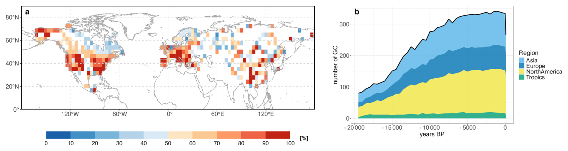
Figure 1(a) Temporal coverage of the REVEALS reconstructions [% of 41 time-steps between 19.5 and 0 ka] and (b) number of available grid cells per continent for each time-step.
2.3 Evaluation of the modern tree cover with remote sensing data
The present-day pattern of simulated and reconstructed tree cover fractions is compared to remote sensing data (MODIS, year 2000–2019; DiMiceli et al., 2022) (Fig. 2). Tree cover in Europe and China is relatively well-represented by REVEALS, whereas REVEALS strongly overestimates tree cover in Alaska, Northeastern North America, and Eastern Siberia, often exceeding 20 %. These discrepancies between MODIS and REVEALS tree cover may provide a first-order indication of the magnitude by which REVEALS could overestimate tree cover due to the reconstruction of vegetation composition only. However, this potential bias is unlikely to be temporally constant, as it depends on changing environmental conditions, vegetation dynamics, and the extent of non-vegetated surfaces.
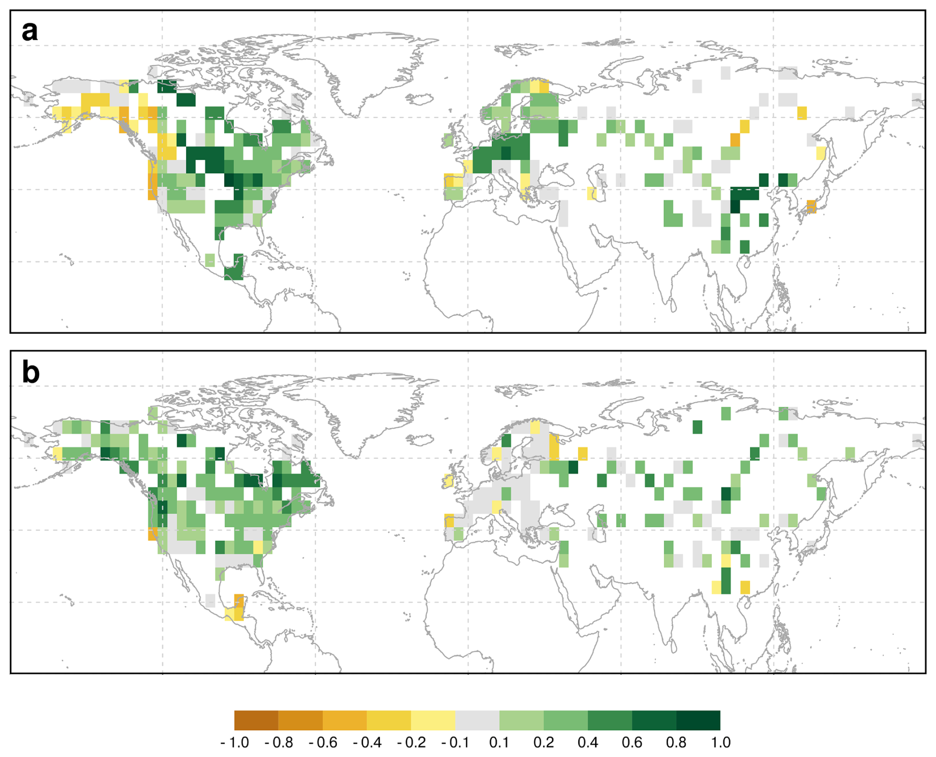
Figure 2Comparison of the (a) simulated and (b) reconstructed tree cover fraction of the modern time-slice with MODIS tree cover (DiMiceli et al., 2022). For MPI-ESM only grid cells for which reconstructions exist are shown.
The MPI-ESM model shows too little tree cover in Alaska and Western North America. However, it significantly overestimates tree cover along the East Asian Summer Monsoon (EASM) margin and in Central and Eastern North America, as well as in Europe. It is important to note that land-use is not included in this version of MPI-ESM, and many of these regions are heavily influenced by historical and contemporary land-use practices, which contributes to overestimated tree cover. Furthermore, validation studies indicate that the MODIS tree cover exhibits substantial uncertainties in boreal and transition regions, particularly at low tree cover fractions (< 20 %) (Montesano et al., 2009), further challenging the comparison with the simulation and reconstructions.
2.4 Comparison metrics
We use three statistical measures for evaluating the similarity of the REVEALS data and the MPI-ESM simulation, the Pearson correlation coefficient, the mean absolute error and the variance difference. The Pearson correlation coefficient (r) is used to assess the similarity in the temporal evolution of the tree cover in each grid cell. It is invariant to differences in the mean and variance. As such, it is well-suited for assessing if the REVEALS data and the MPI-ESM tree cover simulation follow a similar trajectory over time. We consider all grid-cells where the correlation between reconstructions and model data was significant at p < 0.1 in order to maintain spatial representativeness, particularly in regions with sparse data availability and low tree cover where correlations tend to be less statistically significant due to lower signal-to-noise ratios.
In contrast, the mean absolute error (MAE) quantifies the average absolute deviation between the two datasets. As a scale-dependent metric, it is highly sensitive to differences in the temporal mean and amplitude of changes. Consequently, MAE provides a direct measure of absolute agreement and reflects how closely the tree cover values simulated by MPI-ESM aligns in magnitude with the REVEALS-based estimates.
Third, the temporal variance captures the degree of fluctuation or variability within a signal. It complements the other measures by highlighting whether MPI-ESM captures not only the correct magnitude and trend but also the extent of variability inherent in the REVEALS data. We here consider the difference between the variance in the simulated and reconstructed tree cover.
Table 1Different metric groups used in this study. For mean absolute error and correlation, the groups are based on the median (x, here x = 0.45), for the variance difference, the groups are based on a treshold (y) defined ad hoc as 10 % of the overall range (maximum minus minimum) of the variance difference.
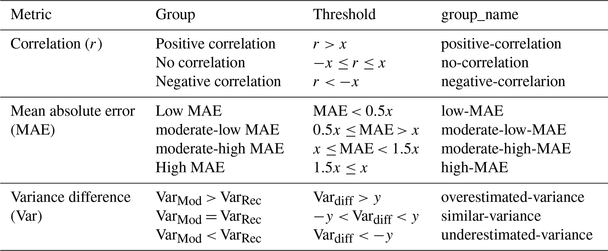
For clarity of presentation, we assign the grid cells for each metric into different groups. For MAE and the correlation coefficient, we categorize the group by thresholds that are multiplier of the median (x) of all values. The variance difference values are categorized into three groups based on a threshold (y) defined as 10 % of the overall range (maximum minus minimum) of the variable. Grid cells with variance difference below this threshold indicate an underestimation of the variance in MPI-ESM compared to REVEALS, those exceeding the positive threshold are indicating an overestimation of the variance compared to REVEALS, and values within the interval ± threshold are defined to be of similar variance. The group definitions are provided in Table 1. Please note that grid cells with non-significant r-values are assigned to the group “no-correlation”.
2.5 Emulation with MPI-ESM simulated climate
To disentangle the effects of precipitation, soil moisture, temperature, and CO2 on the simulated tree cover, we additionally train a statistical emulator to the simulation output of MPI-ESM, following the procedure of Adam et al. (2021). The emulator is based on generalized additive models (GAMs; Wood, 2017), which are non-parametric, non-linear statistical models, in which tree cover is the response variable and mean temperature of the coldest month (Tc), mean temperature of the warmest month (Tw), annual mean precipitation (P), annual soil moisture (Sw), and atmospheric CO2-concentration are used as predictors.
The selection of these variables is motivated by their known importance for vegetation productivity and the implementation of bioclimatic thresholds for Tw and Tc in JSBACH. We train one GAM, which we call emulator in the following, using the data from all grid points, time steps, and climate predictors. Thereby, we estimate the modeled climate-CO2-vegetation relationship across the full climate, CO2, and vegetation gradients, independent of any specific location. This approach is justified by JSBACH modeling the vegetation independently for each grid box, without considering horizontal vegetation interactions such as seed dispersal. We use the function gam in the R package mgcv to fit the emulator (Wood, 2017). Following (Adam et al., 2021), we use a binomial response function due to tree cover being restricted to the interval 0 % to 100 %, and a full tensor product smooth with a cubic regression spline basis for modeling the vegetation-CO2-climate relationship (Wood, 2006). Thereby, we estimate not just the non-linear effects of the individual predictors but also interactions between them. The number of smooth terms was determined with the default optimization routine in mgcv (Wood, 2017). To keep the fitting procedure computationally feasible, we use only every second time step for training.
We simulate sets of surrogate tree cover time series using transient climate forcing by all five variables, and by each individual variable alone, to disentangle the main climatic driver. For the latter, we employ the full emulator but set all predictors to time mean value in the respective grid box. The emulator explain the major vegetation changes over the deglaciation as indicated by predominantly high grid box correlations between the simulated and emulated tree cover (Fig. 3). Lower correlations are mainly concentrated in subtropical South America, the Sahara, arid regions in Asia and the Mediterranean region, and thus include mostly regions with marginal (Sahara) or low changes in tree cover. Marginal tree cover change may lead to spurious correlations, while low correlations in regions with low tree cover changes points to unresolved climate-vegetation dynamics in these regions.
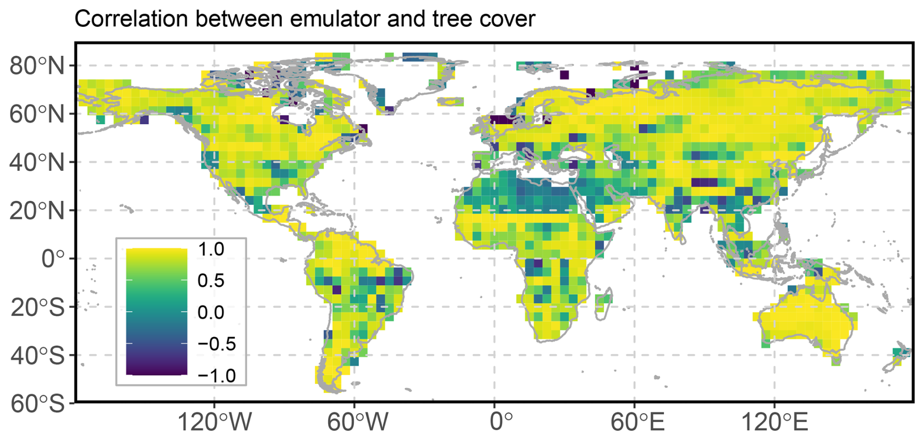
Figure 3Pearson correlation of the emulated tree cover performed with all forcings and the simulated tree cover.
In a second set of emulations, we employ the emulator trained on the MPI-ESM climate and force it with a bias-corrected climate, assuming that grid cell-specific model biases (e.g., related to orography) remain constant over time (Maraun and Widmann, 2018). To construct the bias-corrected climate forcing, we apply the delta method following Beyer et al. (2020), using additive corrections for temperature and multiplicative corrections for precipitation, both downscaled to a 0.5°-grid to align with the CRU-TS 4.08 baseline (University of East Anglia Climatic Research Unit et al., 2024; Harris et al., 2020). Soil moisture was only interpolated to the 0.5°-grid due to the lack of an equivalent observational dataset in CRU-TS 4.08. More details on the preparation of the climate forcing data, time-series and maps for some time-slices are given in the Appendix B.
2.6 Assessing the climate drivers
Complementing the emulation approach, which mimic the response of trees in the MPI-ESM model to climate changes, we assess the non-linearity of climate–vegetation relationships by distinguishing linear from non-linear behaviour. Linear relationships are quantified using Pearson correlation coefficients between simulated or reconstructed vegetation and the individual climate variables. Non-linear relationships are explored using generalized additive models (GAMs; Wood, 2017), with simulated tree cover as the response and the full set of climate variables as predictors. In contrast to the emulations, GAMs are fitted separately for each grid cell here, using 500-year binned datasets smoothed with a Loess filter. Each predictor is represented by a smooth, flexible function capable of capturing curves and other complex patterns. The effective degrees of freedom (edf) associated with each smooth term indicate the degree of non-linearity, with edf ≈ 1 reflecting near-linear relationships and higher values indicating stronger non-linear effects. F-values quantify the importance of each term in explaining variation in the response. For our analysis, we consider only grid cells with edf > 1.2 and p < 0.05, so that we can use the corresponding F-values as indicators of the non-linear climate–vegetation relationships. The most influential variable is identified as the predictor with the highest F-value.
We structure our analysis around a sequence of interconnected questions that progressively link model evaluation with process understanding. We begin by comparing simulated and reconstructed tree cover dynamics from the Last Glacial Maximum to the present (Sect. 3.1), establishing the overall level of agreement between MPI-ESM and REVEALS. Building on this, we quantify and characterize the spatio-temporal differences between both datasets (Sect. 3.2), thereby identifying where and when discrepancies occur.
In a next step, we investigate the underlying mechanisms by analysing the main drivers of tree cover change (Sect. 3.3). This process-based perspective is further refined by explicitly contrasting regions with high and low model–data agreement to assess which factors constrain tree cover dynamics in the model (Sect. 3.4). Finally, we address the question whether a bias-corrected climate can reduce the identified model–data differences (Sect. 3.5), thereby assessing the influence of systematic climate biases on simulated tree cover dynamics.
3.1 Tree cover dynamics in REVEALS and MPI-ESM from the LGM to Present
For the Last Glacial Maximum (LGM), only ∼ 50 vegetation records are available (Fig. 4). REVEALS indicates a predominantly open landscape, consistent with previous reconstructions (Cao et al., 2019a; Davis et al., 2024; Kern et al., 2025; Li et al., 2025a; Prentice et al., 2000). Dense forests occurred mainly in eastern North America (up to 75 % tree cover) and eastern Asia (up to 100 % in Japan), with moderate cover in western North America (up to 60 %). Isolated cells with moderate or high tree cover appear in western central Europe (up to 35 %), the Mediterranean (up to 20 %), Alaska (up to 50 %), and eastern Siberia (up to 20 %). MPI-ESM broadly agrees but shows higher tree cover in Europe and temperate North America, and lower cover in most other regions, including Siberia and the rim of the Tibetan Plateau. The isolated high-cover cells in REVEALS are not reproduced by MPI-ESM, likely reflecting glacial refugia not captured at the model's spatial scale (Leroy et al., 2020).
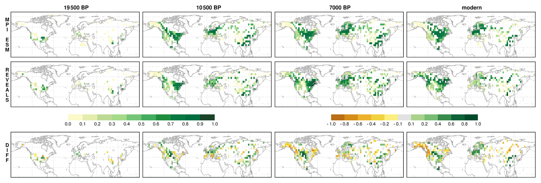
Figure 4Tree cover fraction in MPI-ESM (upper row), REVEALS (second row) and tree cover difference between MPI-ESM and REVEALS (last row) for selected time-slices. A video showing all time slices can be found here (Dallmeyer, 2026).
By 10.5 ka, regions of reconstructed high tree cover expanded markedly. Dense forests developed across eastern North America (70 %–80 %) and western Canada (Pacific coast), and most Siberian records show 60 %–80 % tree cover. Southern China changed little from the LGM, while the northern part of China has experienced a moderate increase in tree cover (30 %–50 %) and up to 70 % in the north eastern part along the Pacific coast. In Europe, REVEALS indicates only modest increases to 30 %–60 %. MPI-ESM captures the general trends but deviates regionally, underestimating forest cover along the North American Pacific coast, in eastern North America's temperate zone, the Mediterranean, and parts of Siberia, while overestimating it in central North America, western and central Europe, northern Siberia, and the East Asian monsoon region.
Towards 7 ka, reconstructions indicate a further increase in tree cover fractions in the Northern Hemisphere north of approximately 50° N, particularly across boreal latitudes and Europe, similar to previous studies (Sweeney et al., 2025). In contrast, MPI-ESM simulates a small but widespread decline, since the maximum Northern Hemispheric tree cover is already reached during early Holocene (Dallmeyer et al., 2022). Exceptions to this trend include periglacial areas in North America and Scandinavia, where tree coverage remains relatively stable or increases slightly. In boreal regions of North America and parts of Siberia, MPI-ESM simulates much less tree cover (∼ 30 % to 80 %) than suggested by the reconstructions. The pattern of disagreement is similar as in 10.5 ka, but much more pronounced in 7 ka. Only in some parts of Europe and eastern North America, tree cover is consistent with the reconstructions, showing dense forests.
At 0 ka, the absence of land-use effects in MPI-ESM likely leads to overestimated tree cover, especially in Europe. Overall, the spatial mismatch between REVEALS and MPI-ESM remains similar to 7 ka: the model simulates too little forest in boreal Asia and North America, but too much in East Asia and central North America.
Overall, MPI-ESM captures the continental-scale patterns and temporal evolution of tree cover reasonably well, but its performance decreases substantially at regional scales.
3.2 Spatio-temporal differences in the tree cover dynamics between MPI-ESM and REVEALS
To identify regional differences between the REVEALS-based reconstructions and the MPI-ESM simulation, we calculate three different metrics (Fig. 5): (a) the Pearson correlation coefficient measuring the synchronicity of the time-series, (b) the MAE measuring the absolute difference in the tree cover estimates and (c) the tree cover variance difference as estimate of differences in the amplitude of tree cover changes. For easier accessibility, we group these measures into statistical categories, aligned on the median value over all grid cells (MAE and r) or the range of the variance difference values (see methods, Table 1).
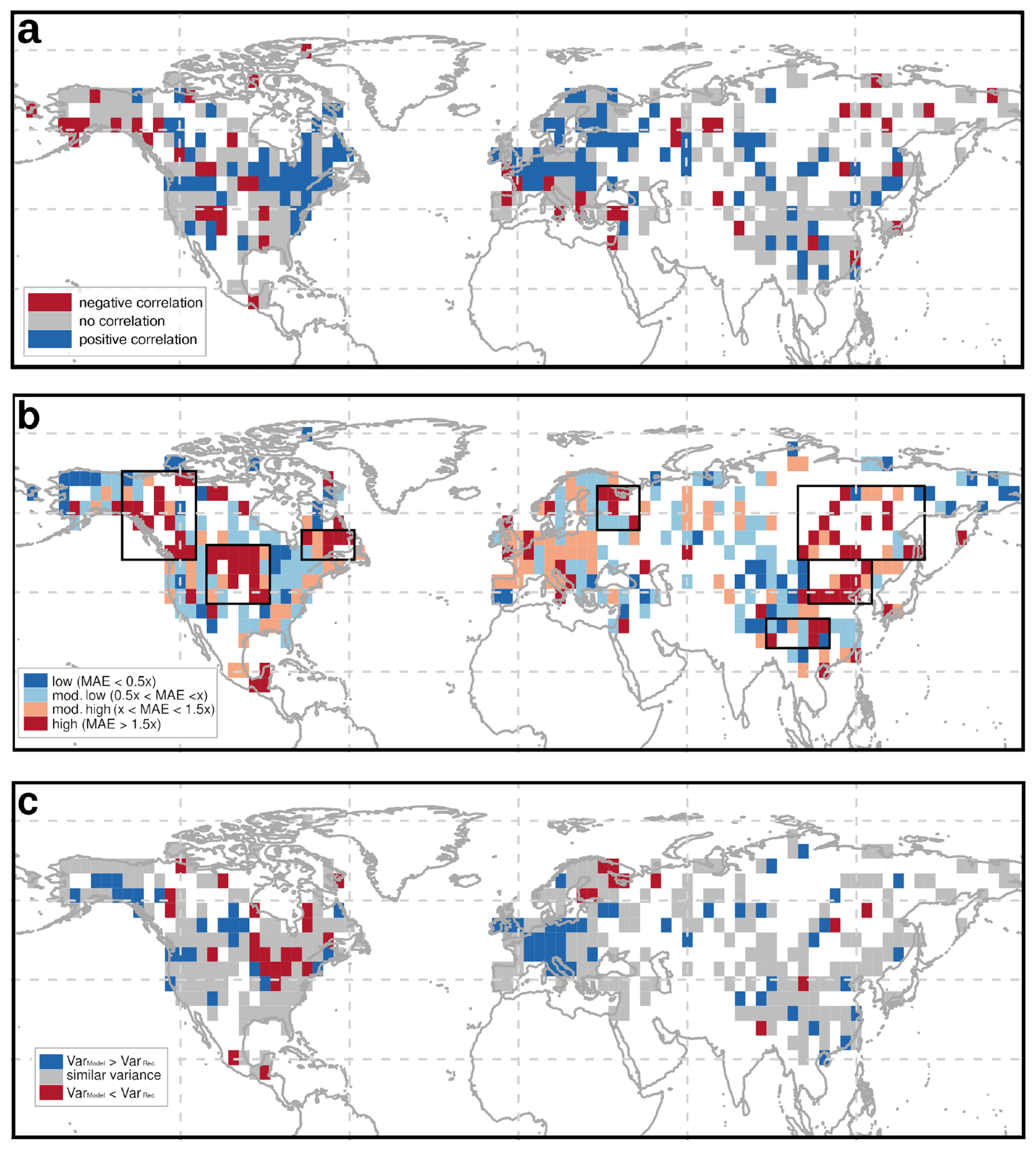
Figure 5Results of different metrics for determining the differences between the simulated and reconstructed tree cover time-series per grid-cells. These are (a) Pearson correlation coefficient, (b) mean absolute error (MAE), and (c) differences in the tree cover variance (Model − Reconstructions). For easier comparability, the results have been grouped in statistical categories by the median value (see Table 1). In panel (b) the regions with highest MAE are marked with rectangles Higher correlation and lower MAE indicate better agreement between simulation and reconstruction, while larger variance differences highlight regions where the model fails to capture temporal variability (blue = model overestimates variance, red = model underestimates variance).
Overall, most of Europe demonstrates a highly positive correlation between REVEALS and MPI-ESM, indicating that the model generally captures the European climate and vegetation dynamics. The Mediterranean region stands out as an exception, experiencing a low or even highly negative correlation. The MAE is moderate for most of Europe, but the model has a higher variance than the reconstructions. These differences could be enhanced by the ignorance of land-use change in Europe which leads to systematic differences in the late Holocene tree cover. However, previous studies report no substantial large-scale human impact on vegetation composition before 2 ka (Roberts et al., 2018; Trondman et al., 2015), thus land use cannot be the only driver of model-data differences. Estimates of potential tree cover for the present time slice indicate more than 80 % tree cover in most parts of Europe except for Spain (Roebroek et al., 2025). This is in line with MPI-ESM.
In North America, mid-latitude regions (40–60°) display a strongly positive correlation, particularly in the eastern part, where also the MAE is low despite a mostly lower variance in the model. However, Central North America exhibits notable weak or even negative correlations and exceptionally high MAE. As the variance difference is low in most grid cells, the high MAE points to a systematic bias and/or diverging trends of the tree coverage in this region. Most grid cells in Western Canada show high MAEs with differing correlations. Coastal regions, also in Alaska, experience negative or weak correlations, while in inland Western Canada correlations are positive in some grid cells only.
In Asia, the correlation indicates no clear pattern, reflecting no robust alignment between REVEALS and MPI-ESM. Siberia displays rather weak or negative correlations, while positive correlations can be observed in non-forested regions, in Western China and along the Pacific coast. Positive correlations are also observed in certain grid cells in Western Siberia. The MAE is high in most grid cells in East Asia, particularly in Central and Eastern Siberia and along the northern rim of the East Asian monsoon region. The variance difference is low in most grid cells, which eliminates amplitude differences as reasons for high MAEs.
These regional discrepancies between the model and the reconstructions point to several key challenges in comparing the REVEALS-based reconstructions with vegetation models. Possible reasons include methodological caveats such as shortcomings in the process of reconstructions, including the REVEALS model (Githumbi et al., 2022; Kaplan et al., 2017; Li et al., 2023b; Schild et al., 2025), biases in the simulated climate, missing or idealized model components (Dallmeyer et al., 2022, 2023; Li et al., 2025a; Zhang et al., 2025) and differences in the vegetation-climate relationship. These factors may lead to local ecological processes, migration lags, and disturbance regimes affecting the reconstructions, while being inadequately represented in the model. This may be particularly problematic in ecotones, where small climatic changes or disturbances can cause large shifts in vegetation composition because multiple vegetation types coexist near their ecological limits.
One important source of divergence lies in the fundamental assumptions underlying each approach: REVEALS estimates plant cover fractions that always sum to 100 % vegetation cover, as it is based on pollen assemblages that represent only vegetated areas without accounting for the proportion of bare ground. Consequently, REVEALS reflects the relative composition of vegetation types within the vegetated area, rather than the absolute area (fi) covered by each vegetation type (i). In contrast, MPI-ESM explicitly calculates both, a bare soil fraction and the composition of plant functional types (ci) on the vegetated area (V), with . While in principle this allows a comparison to REVEALS cover fractions, we have not applied it in this study, because this approach is only valid for regions and time periods where overall tree and vegetation cover is high, such as during the Holocene in Europe (Dallmeyer et al., 2023). In rather open landscapes, this comparison suffers from the artefact of high relative PFT fractions (ci), because for numerical reasons, PFT cover fractions always have to be non-zero in the model. We therefore use the absolute area covered by the PFTs (fi). This fundamental difference (vegetated area vs. vegetation ratios) influences the MAE.
We therefore analyse the differences in tree cover estimates (MPI − REVEALS) grouped by REVEALS tree cover fraction classes. The results demonstrate a clear, non-linear trend across the vegetation gradient (Fig. 6): In areas/time-slices for which REVEALS indicates low tree cover (0 %–20 %), MPI tends to overestimate vegetation cover, with a mean positive bias of approximately 14 %, turning into a negative bias for high REVEALS tree cover classes (−32 % for the 80 %–100 % class). Part of this pattern, however, is methodological, because the difference metric (MPI − REVEALS) is analysed as a function of REVEALS tree cover. This mathematical dependence tends to produce increasingly negative values at high REVEALS fractions even in the absence of ecological effects. The figure should therefore primarily be interpreted as illustrating the magnitude of model–data deviations along the vegetation gradient rather than a purely ecological non-linear response.
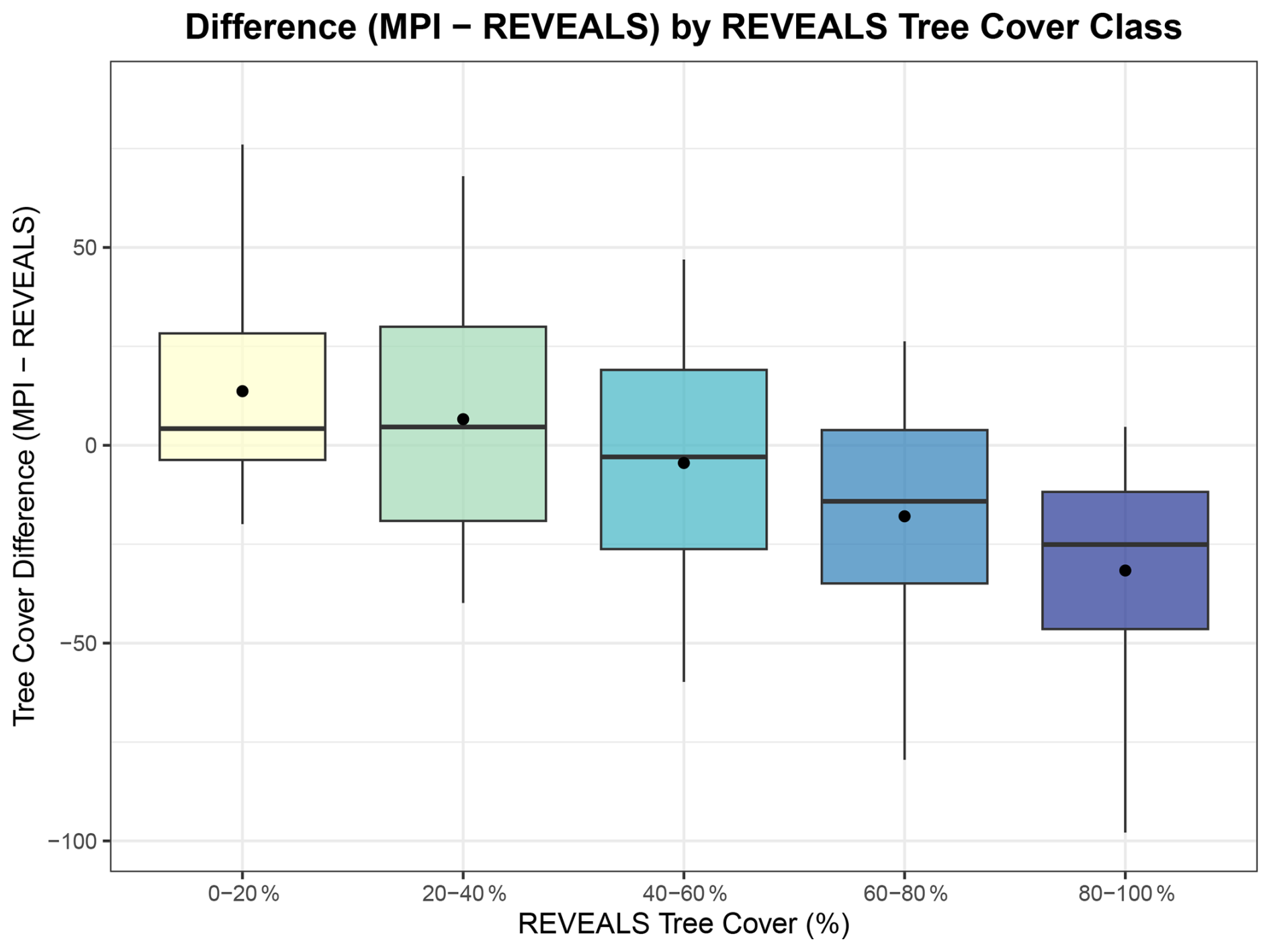
Figure 6Difference between simulated tree cover (MPI-ESM) and reconstructed tree cover (REVEALS) across REVEALS tree cover classes. The boxplots show the distribution of tree cover differences (MP − REVEALS) at any time in relation to the reconstructed REVEALS tree cover class (0 %–20 %, 20 %–40 %, …, 80 %–100 %). The horizontal line in each box indicates the median difference, while the black dot represents the mean. Positive values indicate that the simulation overestimates tree cover compared to REVEALS, while negative values indicate underestimation.
This pattern is nevertheless consistent with the increase in MAE from the LGM (open landscapes) to the Holocene (forested period) (Fig. A3 in the Appendix A) and underlines that the comparison of tree cover fraction of grid cells in the model against tree cover fractions of total vegetation in the reconstructions increase the MAE, particularly in highly forested landscapes.
The positive bias in sparsely wooded regions may result from the model's omission of environmental constraints such as wetlands, permafrost, or water-logged soils, while the negative bias in regions of dense forest may arise from limited number of PFTs, the global, relatively simple definitions of PFTs and their interaction, as well as tuning parameters calibrated for modern rather than past conditions (Dallmeyer et al., 2023; Horvath et al., 2021; Zhao et al., 2025). In addition, the coarse grid resolution of the MPI-ESM leads to a smoothing of regional vegetation patterns. Local maxima, such as tree refugia or areas of particularly dense forest due to local climate conditions, are not adequately captured, resulting in a more homogenized vegetation distribution that overlooks the fine-scale structural heterogeneity evident in the reconstructions.
The differences in absolute tree cover levels expressed by the MAE show a pattern that shares features with the modern deviations to the MODIS observations (Fig. 2, method part). This could point to systematic errors in the REVEALS data and simulation results. REVEALS rather seems to overestimate tree cover in boreal latitudes (Schild et al., 2025) and thus may be too sensitive in cold climates such as glacial periods with open landscapes. Some taxa can occur as trees or shrubs, and their differentiation is not possible based on pollen, especially as the pollen taxonomy was harmonized at the genus level (Herzschuh et al., 2022). More generally, each taxon is assigned to a single plant functional type (PFT), which inherently departs from ecological reality, as many taxa comprise species belonging to different PFTs. Although the reconstruction method by Schild et al. (2025) applies a static threshold that assigns shrub status to common tree taxa (e.g. Betula, Alnus, Corylus) north of 60° N, this adjustment is unlikely to eliminate all biases in tree and shrub PFT representation at northern latitudes. Consequently, the distinction between shrubs and trees in REVEALS may remain imprecise, potentially leading to overestimated tree cover in boreal regions.
On the other hand, the MPI-ESM simulation might suffer from the fixed bioclimatic limits and a tendency towards too cold conditions in the boreal latitudes. For Central North America and the East Asian monsoon margin, the spatial pattern of the MAE diverges from the pattern of disagreement with the MODIS data. In terms of MAE, these regions, which are both forest–steppe transition zones, thus represent the most challenging areas in the comparison.
Many methodological limitations in both the model and the REVEALS reconstructions cannot be quantified directly, and their individual contributions to the model–data tree cover discrepancies therefore remain unresolved. However, we can assess the extent to which systematic climatic biases or differences in the climate–vegetation relationships contribute to the observed mismatches in tree cover patterns. To this end, we analyze the regional climatic drivers of the simulated vegetation dynamics and evaluate which factors distinguish grid cells with close model–data agreement from those exhibiting substantial deviations. Additionally, we employ the trained emulator with bias-corrected climate inputs to further isolate the influence of climatic biases.
3.3 What are the main driver of the tree cover change?
To evaluate the climate–vegetation relationships, we apply a statistical emulator (see Methods) that captures both linear and non-linear responses of vegetation to climatic forcing. To maximize the training data we use the complete global model domain, although reconstructions are limited to the Northern Hemisphere. Pearson correlation coefficients and generalized additive models (GAMs) are additionally used to disentangle the linearity and non-linearity of the climate–vegetation relationship (see Methods). The tested predictors include temperature of the warmest and coldest month (Tw, Tc), annual precipitation (P), annual mean soil moisture (Sw), and atmospheric CO2 (Fig. B1) and we determine the locally most influential predictor as the emulated tree cover curve with the highest correlation to the simulated/reconstructed tree cover. We emphasize that the emulator diagnoses sensitivities intrinsic to the model itself, and thus characterizes model behavior rather than real-world sensitivities.
The emulator results show coherent regional patterns. In high-latitude and high elevation regions (Siberia, Alaska, northern Canada, Tibetan Plateau), the emulation forced with Tw (orange) shows the strongest correlation with simulated tree cover (Fig. 7), consistent with the well-established control of growing-season warmth on vegetation in cold environments (Adam et al., 2021; Dallmeyer et al., 2021; Li et al., 2022a; Seddon et al., 2016; Tucker et al., 2001). In the tropics and subtropics (Africa, South America, Southeast Asia), tree cover is predominantly governed by precipitation (P, light blue), reflecting the central role of water availability (Adam et al., 2021; Gosling et al., 2022; Zhao et al., 2018).
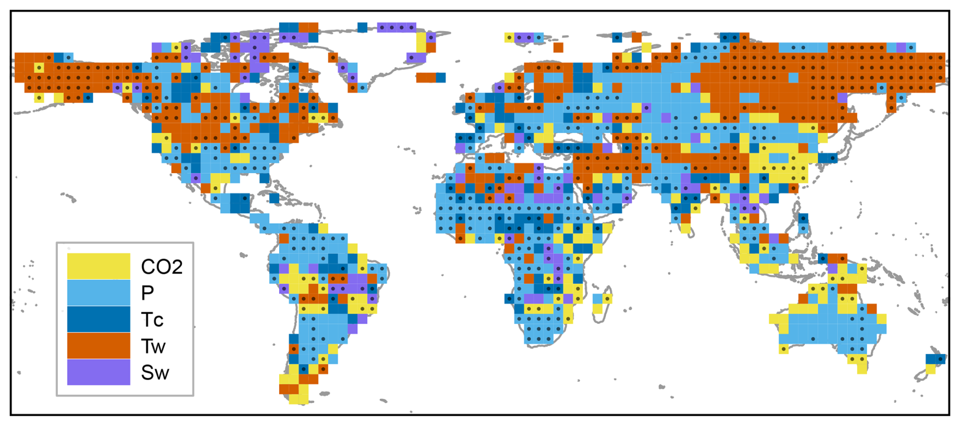
Figure 7Spatial distribution of the most influential climatic variables determining vegetation dynamics across different regions of the world. Each grid cell is color-coded according to the dominant driver of vegetation change in the emulations, which is here based on the emulation with single variable forcing that show the highest Pearson correlation to the simulated tree cover. The variables considered are atmospheric CO2 concentration (yellow), annual precipitation (P, light blue), temperature of the coldest month (Tc, dark blue), temperature of the warmest month (Tw, orange) and annual mean soil moisture (Sw, purple). Grid cells marked with black dots indicate regions where the difference in correlation coefficients between the leading predictor and the second most influential predictor exceeds 0.1 (the median difference), highlighting areas with a comparatively strong dominance of a single driver.
Temperate regions display mixed controls. In Central North America, Tw dominates, whereas in Europe both P and Tc are influential. In large parts of northwestern Asia, precipitation emerges as the primary driver. CO2 (yellow) dominance is spatially scattered, with occurrences in South America, East Africa, Australia, and southern Asia, particularly in the East Asian monsoon region. This strong impact of CO2 has also been found in time-slice-based biome change analysis for the deglaciation period (Tian et al., 2018). However, this relationship should be interpreted as a model-derived sensitivity rather than direct evidence of physiological CO2 fertilisation. The apparent CO2 control may partly reflect a proxy for hemispheric deglacial trends that are not fully captured by the other climate predictors. Soil moisture shows weak influence overall, except in arid regions (e.g. North East Africa) and in tropical monsoon margins.
The spatial patterns inferred from the emulations, correlations, and GAMs are largely consistent and remain robust when the analysis is repeated with a data subset matched to the spatial and temporal structure of the reconstructions. In addition to the dependency of tree cover on Tw in the boreal latitudes, GAMs indicate a non-linear influence of Tc in temperate regions (Central North America and Europe) and around the Tibetan Plateau (Fig. 8c), consistent with physiological evidence that winter cold constitutes a major limitation for tree survival and recruitment. Extremely low temperatures can cause cellular freezing, xylem embolism, and bud mortality, while repeated freeze–thaw cycles and deep soil frost disproportionately damage roots and seedlings (Charrier et al., 2017; Sakai and Larcher, 1987). Juvenile trees, with shallow roots and limited carbohydrate reserves, are more vulnerable than grasses or shrubs, favoring cold-tolerant vegetation. Many temperate species require a chilling period to break dormancy, but excessively low temperatures can exceed frost tolerance and prevent establishment, creating a narrow climatic window for regeneration. In JSBACH, these constraints are represented by PFT-specific minimum-temperature thresholds for the coldest month, below which tree establishment is suppressed, contributing to the non-linear response of trees to Tc.
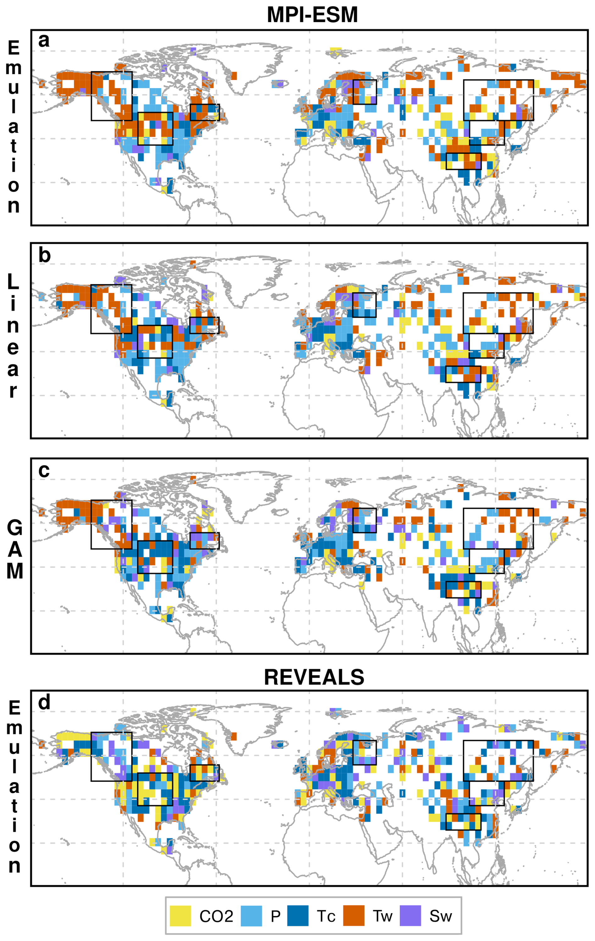
Figure 8Spatial distribution of the most influential climatic variables determining vegetation dynamics according to different methods (Emulation, linear Pearson correlation and GAM) for all considered grid cells in MPI-ESM and REVEALS. The key variables include atmospheric CO2 concentration (yellow), annual precipitation (P, light blue), temperature of the coldest month (Tc, dark blue), and temperature of the warmest month (Tw, orange) and annual mean soil moisture (Sw, purple). Please note that “most influential” means here the variable with the highest R (Pearson correlation) or F value (GAM) or the highest correlation between the emulated and simulated/reconstructed tree cover.
In contrast to the spatially coherent patterns in MPI-ESM, the relationships between reconstructed REVEALS tree cover and emulated tree cover show a much more fragmented structure of climate drivers (Fig. 8d). Moreover, the dominant climatic drivers inferred from REVEALS and the simulated climate differ markedly from those in the model. Most notably, the strong influence of Tw in boreal regions is absent in the reconstructions. Instead, REVEALS tree cover correlates more strongly with P and Tc, even at high latitudes. This finding contradicts the commonly assumed dominance of growing-season temperature in controlling boreal vegetation dynamics and indicate that MPI-ESM does not sufficiently capture the past real-world climate change or that the strong restriction of the extratropical trees by warm season temperature limitations are oversimplified and regionally inappropriate.
A substantial number of grid cells shows the highest correlation of REVEALS tree cover with CO2. Although time-slice experiments have demonstrated a strong impact of the ecophysiological CO2 effect on vegetation differences between the LGM and the present (Claussen et al., 2013; Woillez et al., 2011), the strong correlation between REVEALS-derived tree cover and the CO2 signal in this study rather suggests that the local REVEALS reconstructions follow the overall deglacial warming trend – reflected in the CO2 record – more closely than they follow the simulated local climate or climate-vegetation relationship. This statistical agreement may therefore primarily reflect the shared large-scale deglacial trend in both variables, rather than a direct plant-physiological CO2 response in the real-world.
Because the emulator diagnoses model-internal sensitivities within the MPI-ESM framework, discrepancies between simulated and reconstructed patterns do not necessarily indicate model failure; they may also arise from characteristics of the reconstructions, including their temporal resolution, chronological uncertainties, and spatial aggregation, which can enhance alignment with long-term trends while smoothing local variability.
The dominant climatic drivers in MPI-ESM according to the emulation vary through time. While energy limitations (i.e. Tw or CO2 as most influential variables) are a key driver during the deglaciation, moisture availability (i.e. precipitation and soil moisture dominant driver) becomes increasingly important toward the Holocene (Fig. 9). The moisture availability influence peaks at 7.5 ka, indicating a widespread shift from energy- to water-limited environments in the early Holocene before shifting back to higher energy-limited influences in the late Holocene. The reconstructions reflect the transitions between energy- and water-limited regimes (in terms of their correlation with the emulations), with a maximum area of water-limited regimes reached at 8.5 ka. The influence of Tc stays relatively constant through time in the simulations, whereas it increases by ∼ 10 % in the Holocene in the reconstructions.
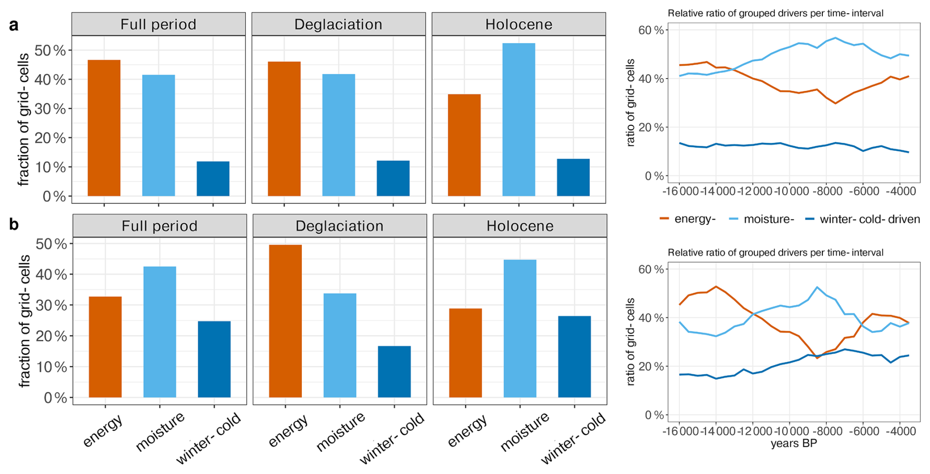
Figure 9Summary of the climate drivers (averaged over all grid cells) for different periods and their evolution over time (moving average over 15 time-steps = 7500 years) for (a) MPI-ESM and (b) the REVEALS-based reconstructions (vs. simulated climate). For easier interpretation we merged the climate drivers into the groups representing energy-limited (Tw and CO2), moisture-limited (Sw and P) and winter-cold-limited (Tc) regimes.
3.4 What constrains tree cover dynamic in the model – High- vs. low-agreement grid cells?
Based on the correlation, mean absolute error (MAE), and variance differences between simulated and reconstructed tree cover, we classify all grid cells into statistical categories (cf. Fig. 5 and Table 1) and analyse differences in tree cover responses to climate change among these groups. Additionally, we assess whether the observed group differences arise from insufficient data (e.g., incomplete or short time series) or are related to geographic position (latitude or longitude), and whether they affect the representability of the tree cover dynamic by the emulation. To this end, we pre-select variables that show significant differences between the groups based on pairwise comparisons using the Wilcoxon rank-sum test (Appendix C, Table C1 in the Appendix C). Then, we use this preselection of predictors for running a PCA-analysis to determine the most influential variables for group-separation.
It should be noted that high MAE values and low correlations do not necessarily indicate deficiencies in the climate-vegetation relationship in the model. They may also reflect the fact that the reconstructions capture local ecological processes, migration lags, or microclimatic conditions that are not represented in the coarse-resolution simulation. Since these factors cannot be filtered out, all grid cells are included in the analysis to examine the dependence on climatic conditions.
Grid cells exhibiting a synchronous dynamic in simulated and reconstructed tree cover (positive correlation-group) differ markedly in their tree cover response to climate change from those with negative correlations (Fig. C1 in the Appendix C). High agreement occurs where both simulated and reconstructed tree cover follow the simulated climate linearly as indicated by strong Pearson correlations with CO2, precipitation (P), soil moisture (Sw), and temperature of the coldest month (Tc). In these cells, Tc shows high correlations with precipitation (r ≈ 0.85), which itself closely follows CO2 changes (r ≈ 0.7). The temperature of the warmest month, in contrast, is only moderately correlated with CO2 and precipitation (r ≈ 0.45 and r ≈ 0.3). Good agreement can also arise in cells with more non-linear responses to precipitation, which the GAM analysis identifies as the main driver in significantly more cells of the positive-correlation-group than in the negative-corelation-group. In contrast, disagreement (negative correlation) is linked stronger to non-linear responses to Tw, which emerges significantly more often as the main driver in grid cells of the negative-correlation–group according to the GAM analysis. In grid cells of the negative-correlation-group, Tw is furthermore rather negatively correlated with CO2. Neither the variance difference nor the MAE are deviating significantly between grid cells in the negative- and the positive-correlation-group. The agreement is furthermore independent of the time-series length, including the timing of the first data point and the number of missing values.
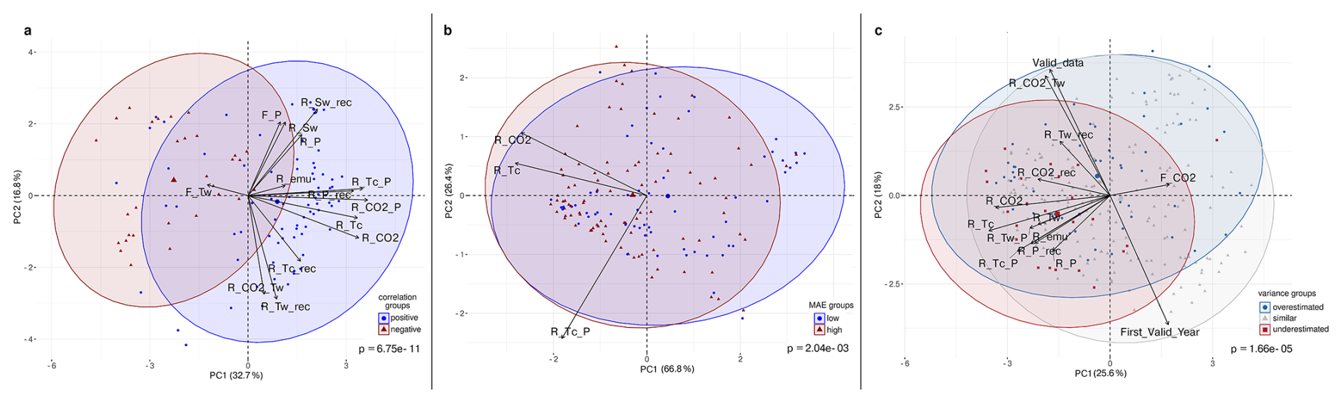
Figure 10Principal Component Analysis (PCA) biplot of climate–tree cover relationships for key-climate variables in grid cells with (a) positive (blue) and negative (red) correlations, (b) low (blue) and high (red) MAE and (c) overestimated (blue), underestimated (red) and similar (grey) variance between simulated and reconstructed tree cover. Arrows indicate the direction and strength of climate-related variables contributing to the ordination. Hereby, “F_” corresponds to the F-coefficients in the GAM-analysis (i.e. non-linear relationship) and “R_ ” to the Pearson correlation coefficients (i.e. linear relationship) in the “model”, the reconstructions (“_rec”) or in the emulation (“_emu”). The considered variables are precipitation (P), soil moisture (Sw), temperature of the coldest (Tc) and warmest (Tw) month and CO2. For instance, R_Tw_rec corresponds to the Pearson correlation coefficient for reconstructed tree cover and simulated Tw, while R_CO2 corresponds to the Pearson correlation coefficient for the simulated tree cover and CO2. Significance is tested via Wilcoxon test (a, b) or Kruskal-Wallis test (c).
The PCA on the preselected key variables (F-statistics and Pearson correlations) confirms the significant (Wilcoxon test, p = 6.75 × 10⁻¹¹) separation between the correlation-groups, with PC1 and PC2 jointly explaining 49.5 % of the variance (Fig. 10a). High agreement aligns with strong positive loadings of the Pearson correlation coefficients between tree cover and CO2 and Tc, as well as the strong positive precipitation-CO2- and precipitation-Tc-correlations, which most strongly differentiate the positive-correlation-group. In contrast, the non-linear response to Tw is clearly oriented towards the centroid of the negative-correlation-group (negative loadings on PC1), substantially contributing to its separation from the positive-correlation-group. Other variables (including the linear and non-linear relationship to precipitation (R_P, F_P), and correlation to soil moisture (R_Sw) load mainly on PC2 and play only a minor role in distinguishing the groups.
MAE groups do not match with any correlation-group classification. However, grid cells with low MAE differ in climate response from high-MAE cells typically located at mid-latitudes (∼ 50° N) (Fig. C2 in the Appendix C). In the mean, grid cells with early starting reconstructions have a significantly lower MAE than grid cells with later starting reconstructions. High-MAE cells exhibit significantly higher linear correlations of the simulated tree cover with Tc and CO2. No significant differences in dominant climate drivers are found between the MAE groups, indicating that the prevalence of a particular variable as the main driver does not systematically vary with model error. The PCA of MAE groups (PC1 66.8 %, PC2 26.4 %) confirms the statistically significant (Wilcoxon test, p = 2.04 × 10⁻³) separation, mainly by the linear correlation to Tc, and CO2.
For the tree cover variance difference, we compare all three groups. Grid cells with overestimated variance in the model are characterized by earlier, more complete time series, stronger linear correlation with CO2, and Tc, and also higher correlations between precipitation and CO2 and Tc compared to grid cells with similar variance (Fig. C3 in the Appendix C). Moreover, overestimated variance co-occurs with much higher linear correlation between Tw and CO2 (r ≈ 0.6), but can be less well represented by the full-forcing-emulator.
Grid cells with underestimated variance in the model mainly cluster in Eastern North America and show higher linear correlations with Tw, Tc, P, and CO2 and lower non-linear relationship to Sw, Tw and CO2 compared to grid cells with similar variance. Consistently, correlation between P and CO2, Tw and Tc are significantly higher compared to grid cells with similar variance. Interestingly, grid cells within both groups (overestimated and underestimated variance) exhibit higher correlations between simulated and reconstructed tree cover than grid cells with similar variance, despite larger MAEs. This indicates that the temporal structure can be preserved even when variability and amplitude is misrepresented. The lower correlations and low MAE in the group with similar variance points to poor temporal coherence despite a reasonable magnitude fit.
The PCA of the preselected variables confirms the significant separation between the variance groups (Kruskal-Wallis, p = 1.66 × 10⁻⁵) in their multivariate environmental characteristics, with PC1 and PC2 explaining 43.6 % of the variance. Along PC1, the most influential contributors to group separation are the contrasting non-linear vs. linear responses of the tree cover to CO2. The non-linear relationship to CO2 (F_CO2) loads positively and aligns with the overestimated-variance–group, while the linear correlation to CO2 exhibits negative loadings associated with the underestimated-variance–group. Additional separation along the horizontal axis arises from variation in linear correlations with Tc, Tw, and P, which load negatively towards the underestimated-variance-group. Separation along PC2 is driven primarily by differences in the Tw–CO2 relationship and by the length of the time-series.
Overall, these analyses show that the agreement between simulated and reconstructed tree cover is strongly influenced by the choice of evaluation metric and the specific ways in which vegetation responds to climate drivers. The temporal evolution is best captured when tree cover responds linearly to the hemispheric warming and moistening trends, reflecting the coherent signal shared by precipitation, cold-season temperature, and the global CO2 trajectory. In these grid cells, reconstructed tree cover appears to follow the large-scale trend closely, probably indicating regions where vegetation dynamics are primarily controlled by broad-scale climatic forcing and are therefore well captured by the model.
In contrast, grid cells in which a non-linear response to summer temperature fosters poor temporal correlations could coincide with regions in which the reconstructions indicate strong regional or local vegetation trajectories that are not governed primarily by hemispheric climate forcing. This pattern suggests that the mismatches to REVEALS do not necessarily arise from shortcomings in the model's representation of large-scale vegetation–climate interaction, but rather highlights areas where regional ecological or climatic processes play a comparatively larger role, influencing the reconstructions.
MAE reflects differences in simulated tree cover sensitivity to cold-season temperature and CO2, with greater disagreement when tree cover is more linearly aligned with Tc and CO2. Deviations in variance do not increase model–data asynchronicity but tend to coincide with higher MAE, indicating that the timing of changes can be accurately reproduced even when amplitude is misrepresented. Strong linear correlations with CO2 lead to overestimated variance, whereas non-linear relationships tend to produce underestimated variance. Overall, the response of the climate–vegetation system to CO2 forcing emerges as one key controlling factor. Linear alignment of climate with the CO2 signal co-occurs with synchronous tree-cover changes in reconstructions and MPI-ESM, but simultaneously increases MAE and exaggerates amplitudes in the model, pointing to a too strong sensitivity of forests to CO2 variations in MPI-ESM. This high sensitivity to CO2 in MPI-ESM has also been observed in other studies (Arora et al., 2020; Kleinen et al., 2023a; Rogers et al., 2017).
3.5 Can we reduce the biases by prescribing a bias-corrected climate?
The trained emulator is forced with a bias-corrected climate to test the impact of potential, systematic climate offsets on the tree cover change. The bias-corrected climate and examples of the resulting tree cover emulation in comparison with the original simulation is provided in Figs. B1–B3 in the Appendix B. To evaluate where the bias-corrected emulation enhances model-data agreement (i.e. it shows higher r or lower MAE values or variance differences), we statistically compare the distribution of grid cells with relative improvement (> 25 % percentile) or worsenings (< −25 % percentile) for the correlation-, MAE-, and variance-groups, using the same classification as in Fig. 5 and Table 1. Note that a relative improvement in model-data agreement does not necessarily imply a good absolute agreement, as r or MAE values may still indicate substantial discrepancies.
The bias correction enhances the model–data agreement at the regional scale, but not in the mean across all grid cells. Correlation coefficients and variance differences improve in only about one third of the grid cells, and the MAE improves in roughly 40 %, while around 25 % of the grid cells in all groups remain unaffected, respectively. The remaining cells show deteriorated performance. MAE improvements (blue areas, Fig. 11) concentrate in Western/Central North America Scandinavia, Southern Europe and Eastern Asia and mostly coincide with an increase in the tree cover correlation, except for Asia. Variance differences increase across much of North America, Europe, and China, but decrease north of 40° N in Asia and south of 40° N in North America, pointing to a high degree of regional sensitivity in the model's ability to reproduce reconstructed variability patterns. The bias correction is most effective in grid cells with initially poor performance, such as those exhibiting negative correlations, high MAE, or large variance mismatches. For correlation and variance, the improvements show no systematic association with the dominant climate driver, suggesting that errors in these metrics are broadly distributed and more difficult to correct with this kind of bias correction. In contrast, MAE improvements occur disproportionately more in grid cells where temperature (Tw) is the primary driver, while deteriorations are more frequent in precipitation-dominated (P) cells.
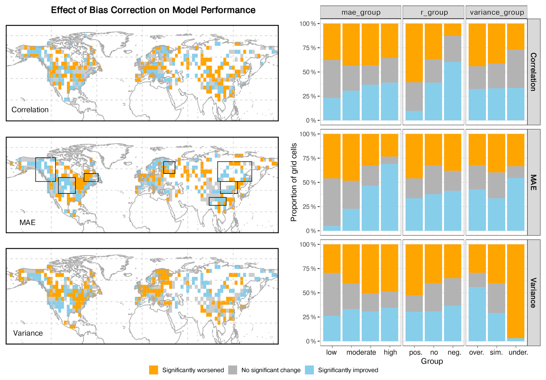
Figure 11Impact of the bias correction on the three performance metrics (correlation, MAE, and variance). The left panels display spatial distributions of significant changes in these metrics after bias correction. Blue indicates relative improvement compared to MPI-ESM (> 25 % percentile), orange relative worsening (< −25 % percentile), and grey no change. The right panels summarize these effects by showing the proportion of grid cells with each type of change across the different model-performance categories (mae-, correlation- and variance-groups). Note that a relative improvement (blue) does not necessarily imply good absolute agreement; it only indicates better agreement in the emulation compared to the original MPI-ESM simulation.
The results indicate that MPI-ESM performs reasonably well at the hemispheric scale, so that regional bias corrections often come at the expense of other areas, producing localized improvements but limited overall gain. The corrections primarily reduce large systematic errors, leading to improvements in MAE and correlation, but they do not consistently preserve the amplitude of variability, and variance is degraded across large areas. Consequently, the bias-correction methods tend to redistribute errors rather than uniformly improving the model performance across the domain. Furthermore, tree-cover dynamics driven by temperature are more amenable to correction, whereas precipitation-driven dynamics remain more sensitive and are more likely to deteriorate under bias correction, reflecting the differing spatial and temporal characteristics of these climate drivers.
To better understand the regional behaviour, we compare the time series of tree cover fractions (Fig. 12) from reconstructions (red), the MPI-ESM simulation (black), and statistical emulations (blue) with bias correction for the six regions with the largest MAE. Overall, the (bias-corrected) emulated tree cover aligns better with the reconstructions than the simulation in most high-MAE regions. Particularly, in the temperate forest–steppe transition zones in Central North America and Northern China (EASM margin), the emulation produces substantially lower tree cover and aligns more with the reconstructions than the simulation, indicating that the large simulation–reconstruction discrepancies in these regions mainly stem from systematic climate biases.
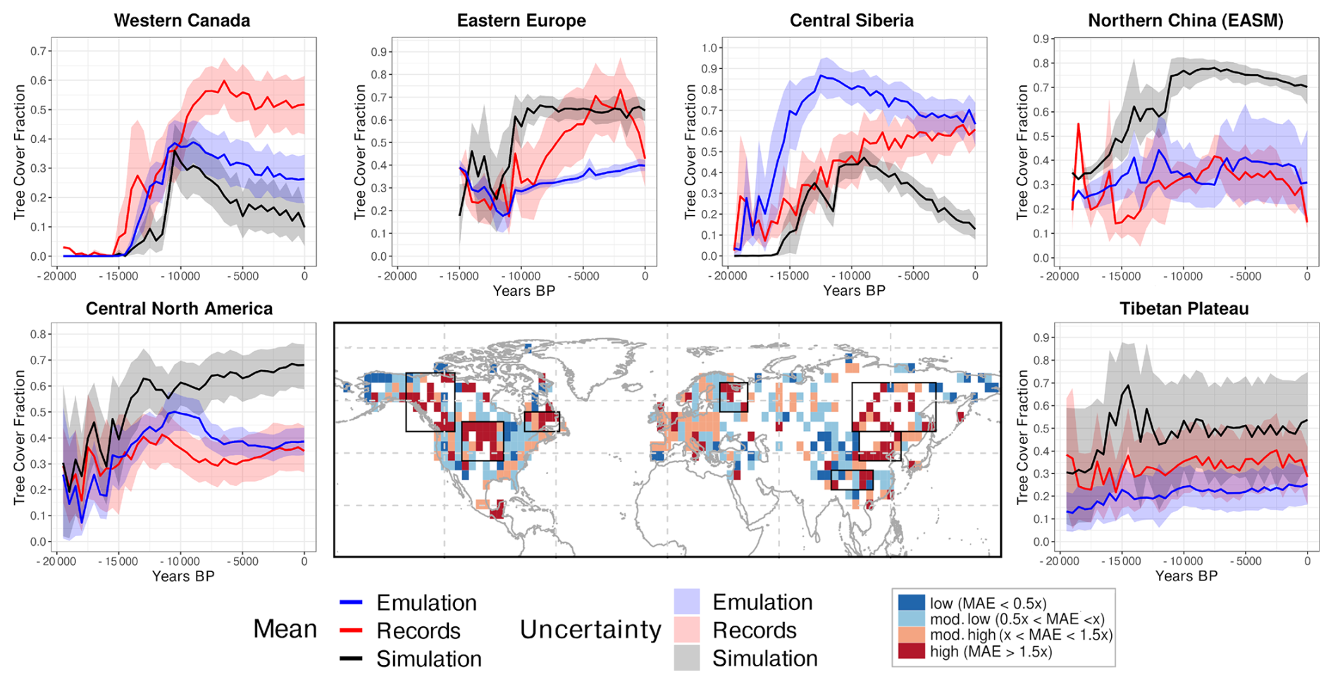
Figure 12Comparison of reconstructed (red), simulated (black), and emulated (blue) tree cover fraction over the past 19 500 years in six selected regions, i.e. the regions indicating the highest MAEs between the simulated and reconstructed tree cover. Shaded areas represent uncertainty, assessed via bootstrapping. The central panel shows the spatial distribution of the MAE between simulated and reconstructed tree cover (see Fig. 5), classified into four categories: very low, low, moderate, and high. Regions outlined with black boxes correspond to the locations of the time series plots. Please note that for Northeastern North America, no time-series are shown since the time-series are relatively short there.
In Western Canada, bias-corrected warmer summers advance postglacial tree-cover growth and reduce offsets with reconstructions by 30 %, but neither simulation nor emulation capture the mid-Holocene maximum. The model appears to miss the prolonged early- to mid-Holocene warming, pointing to deficiencies in the simulated climate trajectory
In Central Siberia, the bias correction increases emulated tree cover too strongly during deglaciation and leads to a too early peak, indicating an overestimated sensitivity to warm-month temperature and explaining the worsening of the correlation despite an improved MAE in this region. The simulation with much lower temperatures agrees with reconstructions until 9.5 ka, after which their trends diverge, while the emulation and reconstructions only converge in the late Holocene. Neither simulation nor emulation reproduce the reconstructed Holocene increase, pointing to a wrong driver or structural vegetation deficiencies in the model. This mismatch may partly be caused by the missing permafrost processes in this version of MPI-ESM. Permafrost is a major regulator of tree cover across northern high-latitude regions, including Siberia, western Canada, and Alaska. It controls soil thermal and hydrological conditions that limit tree establishment and growth (Cao et al., 2019b; Helbig et al., 2016; Jin et al., 2022, 2021; Kruse et al., 2022; Stuenzi et al., 2021), influences fire regimes (Kim et al., 2024) and shapes forest–tundra mosaics (Viereck, 1973) that may decrease the absolute forest cover in the REVEALS reconstructions. Thus, permafrost can maintain unsuitable ground conditions and can cause significant temporal lags in postglacial forest expansion (Herzschuh et al., 2016; Li et al., 2022b; Tian et al., 2018).
In Eastern Europe, bias correction slightly improves pre-Holocene agreement, but the emulation substantially underestimates Holocene tree cover and fails to capture the reconstructed mid-Holocene rise and 4 ka maximum. This indicates that the model-data mismatch in this region is not related to systematic climate biases. Tree cover in the emulation closely follows the precipitation that is much lower in the bias-correction than in the simulation. This strong relationship may be incorrect, but also none of the other considered climate variables indicate a mid- to late-Holocene peak that could explain the reconstructed late tree cover maximum.
On the Tibetan Plateau, warmer conditions in the emulation would raise tree cover, but reduced precipitation limits its growth. Nonetheless, emulated trends better match reconstructions, highlighting the combined influence of multiple climate variables on tree-cover dynamics and that JSBACH in principle captures the vegetation-climate relationships in this region well.
Overall, bias correction is most effective in regions with strong model–data mismatches, where systematic climate biases are the main cause of discrepancies, such as in Western Canada, Central North America or Northern China. In these regions, the MAE can be substantially reduced, but whether the correlation to the reconstructed tree cover is improved, depends on the relationship between the climate variables and there joint effect on the tree cover. The interactions among climate variables (or with CO2) are often non-linear, so that changes in one variable can alter the importance or sensitivity of the tree cover response to another. Significant mismatches persist in regions where non-climatic factors, such as missing processes in the model, cause the mismatch (Eastern Europe, Central Siberia). The effectiveness of bias correction is further limited in regions with inappropriate climate-temperature relationships, either due to incorrect dependencies or an overestimated tree-cover sensitivity to temperature changes. In addition, the applied bias correction can not reduce errors in the temporal temperature evolution. Therefore, the mismatch in the timing of the Holocene tree cover maximum persists across large parts of the Northern Hemisphere in the emulation with bias-corrected climate, particularly in boreal latitudes. This can partly be expected because the applied bias correction removes only stationary offsets.
At the same time, the results indicate that the absence of a mid-Holocene vegetation maximum is unlikely to be explained solely by biases in the simulated climate. Instead, they point toward structural limitations in the representation of boreal vegetation dynamics and associated land–surface feedbacks in the model, which the emulator does not correct for.
This interpretation is consistent with findings from transient Holocene simulations. Several studies highlight the importance of vegetation feedbacks for Holocene climate evolution, in particular mid-Holocene warmth in the Northern Hemisphere (Thompson et al., 2022). However, models with dynamic vegetation frequently underestimate the magnitude and spatial extent of vegetation changes inferred from proxy records (Dallmeyer et al., 2019; Harrison et al., 2015; Tian and Jiang, 2013), potentially limiting the strength of these feedbacks.
Transient Holocene simulations also show strong regional differences in the timing and magnitude of the Holocene Thermal Maximum, particularly in boreal regions. While models agree reasonably well in regions strongly influenced by residual ice sheets, substantial model–proxy discrepancies persist in areas such as Alaska and Siberia (Zhang et al., 2017, 2018). In these regions, simulated temperature trends during the Early Holocene often differ from pollen-based reconstructions (i.e. warming in reconstructions, cooling in models), highlighting persistent uncertainties in both climatic forcing of vegetation and regional feedbacks (Hao et al., 2025).
In addition, the varying impact of bias correction across regions and time periods may at least partly result from the fact that different climatic factors constrain vegetation at different times. While temperature corrections may improve model–data agreement particularly during the deglaciation, Holocene mismatches may relate to insufficient representation of precipitation dynamics.
Over the last 20 000 years, global warming, driven by orbital changes, rising CO2, and ice sheet retreat, caused major shifts in climate and a reorganisation of vegetation. While pollen-based reconstructions show significant biome shifts since the Last Glacial Maximum (LGM), the vegetation dynamics and the impact of the climate drivers on the vegetation dynamics remain unclear. The new large-scale pollen-based reconstruction for the Northern Hemisphere by Schild et al. (2025) provides a valuable basis for evaluating Earth system models as it provides quantitative, gridded tree cover reconstructions, improving the comparability to the model output and therewith our understanding of vegetation responses, model-data mismatches, and model performance. We have compared this dataset with a transient simulation by the Max-Planck-Institute Earth System Model MPI-ESM (Kleinen et al., 2023a, b) to answer the following questions:
- a.
How well does the model reproduce reconstructed tree cover patterns?
Pollen-based REVEALS reconstructions show regionally variable tree cover during the Last Glacial Maximum (LGM), with high values in parts of eastern North America and Asia. Tree cover expanded markedly during deglaciation, especially north of 50° N. While MPI-ESM broadly captures these trends, it simulates consistently higher tree cover in Europe and East Asia and lower tree cover in boreal North America and Siberia. MPI-ESM tends to simulate too high tree cover fractions in sparse forest and too little tree cover fractions in dense forests. Discrepancies are most pronounced from mid-Holocene to present, partly due to missing land-use in MPI-ESM. Reconstructed and simulated tree cover show overall strong correlations in Europe, except in the Mediterranean. North America and Asia indicate regional mismatches, with high MAE in Siberia, the boreal latitudes in America and the forest-steppe transition zones in Central North America and East Asia.
- b.
What are the drivers of the tree cover dynamic?
Statistical emulator and correlation analyses demonstrate clear regional patterns in the climatic controls of simulated vegetation. In high latitudes, summer temperature is the dominant driver, while in tropical and subtropical regions, precipitation is key. In temperate zones, both temperature and precipitation are important, with regional differences. MPI-ESM shows consistent spatial patterns, but the comparison with REVEALS reconstructions indicates notable discrepancies. For REVEALS, simulated precipitation and cold season temperature and the CO2 change better explain tree cover changes – even in boreal regions – contrasting with the model's emphasis on warm season temperature. This suggests limitations in MPI-ESM's climate simulation or bioclimatic assumptions. Both, reconstructions and simulations show a shift from energy-limited regimes during the deglaciation to moisture-limited regimes during the early and mid-Holocene, followed by regrowth of energy-limited areas in the late Holocene.
- c.
Can we infer differences in the climate-vegetation relationships between areas with model-data agreement and model-data-disagreement?
We note that low model–data agreement does not necessarily indicate model deficiencies, but may also reflect local processes mirrored in the reconstructions. Moreover, our analysis indicates that grid cells with high model-data agreement in the tree cover dynamic differ significantly in their climate sensitivity from those with poor agreement. High correlations are associated with a largely linear vegetation response to multiple climate drivers in the model, including CO2, precipitation, soil moisture, and cold-season temperature. Vegetation dynamics in these grid cells are dominated by the overall (hemispheric) deglacial warming trend. The precipitation and cold season temperature themselves are strongly correlated with the CO2 signal. In contrast, poor agreement is often linked to more complex, non-linear responses dominated by summer temperature, and rather indicate regional tree cover trajectories.
Grid cells with high MAE cluster in the mid-latitudes and the time-series start later. Interestingly, high-MAE cells exhibit stronger correlations with cold-season temperature and CO2, suggesting a too strong sensitivity of the tree cover to CO2 in the model. The dominant climatic drivers, however, do not differ systematically between the high- and low-MAE- groups.
Grid cells where the model overestimates variance show strong linear correlations between tree cover and CO2 or Tc, as well as stronger P–CO2 and Tw–CO2 linkages than grid cells with similar variance. Likewise, cells where variance is underestimated exhibit stronger correlations with Tw, Tc, P, and CO2 than cells with similar variance. Variance biases mainly reflect the tree cover response to CO2 changes: Linear responses lead to overestimation, non-linear responses to underestimation, suggesting a too strong sensitivity of the tree cover to CO2 changes in MPI-ESM. Notably, grid cells with similar model-data variance have lower tree cover correlations and lower MAEs than the other groups, indicating low temporal coherence and demonstrating that correct amplitude does not guarantee realistic dynamics.
- d.
What can we learn from this study?
Global vegetation modelling with Earth System Models remains challenging, as these models prioritize broad climatic functioning over detailed regional patterns. While the model captures the major large-scale shifts from open LGM landscapes to Holocene forests, the regional dynamics are often misrepresented, showing low correlation with reconstructions or mismatches in variability and absolute cover. Reconstructions typically use regionally differentiated definitions and vegetation characteristics to aggregate thousands of taxa, whereas global models rely on broad plant functional types constrained by universal, static bioclimatic limits derived from modern human-affected vegetation. These fixed bioclimatic limits in the models seems to lead to a too strong dependence of the simulated vegetation on the warm season temperature and to a misrepresentation of the non-linear tree cover response to climate. Furthermore, the sensitivity of the tree cover response to CO2-changes seem to be too strong in this model version, expressed by higher MAEs and overestimated variance under strong linear coupling of the tree cover to CO2. Our study also shows that the climate–vegetation relationship can regionally be well captured but that systematic climate biases can still produce large mismatches between simulated and reconstructed tree cover. Two mechanisms may contribute to these discrepancies. First, deficiencies in simulated climate trajectories can lead to incorrect climate forcing of the vegetation model. In the temperate forest–steppe transition zones of Central North America and East Asia, the model is systematically too wet, enabling tree growth much earlier than observed and causing major offsets. Bias correction can reduce the mismatch to the reconstructions here. At high northern latitudes, the model is too cold and warm season temperatures peak during the early Holocene, which distorts the simulated climate forcing of tree cover and contributes to unrealistic vegetation dynamics, e.g. in Western Canada.
Second, limitations in vegetation sensitivity to climate may further amplify these mismatches. In combination with the global and fixed bioclimatic thresholds used in the vegetation model, the cold bias likely alters the tree cover sensitivities to temperature in JSBACH (and thus in the emulator trained on it). As a result, bias correction does not improve the agreement with the reconstructions in all boreal regions, but instead increases the model-data mismatch, e.g. in Siberia, indicating a misrepresented climate forcing and an unrealistic representation of the boreal forest dynamic. Missing processes in the model, such as the impact of permafrost on the tree cover dynamic, further increase the model-data differences. Consequently, the model is not able to capture the mid-Holocene forest maximum observed across large parts of the Northern Hemisphere. Instead, tree cover peaks during the Early Holocene in the model due to the strong sensitivity of the simulated tree cover to warm season temperature, which closely follows the insolation forcing. However, the underlying mechanisms and consequences require further analysis and will be addressed in a follow-up study.
In addition to the sources of error in the model, the reconstruction method has shortcomings that are not explicitly discussed here. However, the question arises to which extent REVEALS is suitable for reconstructing forests in open landscapes. Especially in regions with sparse forests, such as the boreal latitudes, REVEALS greatly overestimates the proportion of forest. The fact that bare ground cannot be estimated is problematic and contributes to the model-data mismatch.
- e.
How can we improve Dynamic Vegetation Models to better simulate past and future tree cover changes
Current Dynamic Vegetation Models (DVMs) capture global vegetation responses and their role in the climate system, but they are less reliable for detailed regional or local vegetation patterns, particularly with the low spatial resolutions used in ESMs. Most DVMs employ overly simplified soil schemes and lack explicit representation of permafrost processes. In cold and arid regions, vegetation dynamics are often constrained by soil processes and not just by climate. Without realistic soil and permafrost modeling, DVMs tend to overpredict tree establishment at treelines or in permafrost peatlands, leading to inaccurate biogeographical predictions.
Vegetation dynamics are rarely linear and are often governed by unknown or context-dependent thresholds. Transition zones between biomes are particularly difficult to model due to complex interactions of multiple limiting factors. Dynamic thresholds, rather than static ones, are essential to capture these processes more accurately.
Plant Functional Types (PFTs) are often too coarse to capture regional vegetation responses, especially under strongly changing climatic conditions or in transition zones between biomes. By grouping species into broad categories, PFTs can overlook important differences in traits that determine survival, growth, and reproduction under stress, such as drought tolerance, frost resistance, rooting depth, or fire-adaptive characteristics. Trait-based approaches, in contrast, allow models to explicitly represent these functional differences and the variability within species or populations, but are still in an early phase of development. They would enable a more mechanistic simulation of how vegetation responds to environmental changes.
Improving DVMs for palaeoclimate studies, thus, requires (i) integrating realistic soil and permafrost dynamics, (ii) accounting for non-linear processes and dynamic thresholds, (iii) enhancing disturbance modules, (iv) moving from static PFTs to trait-based or individual-based approaches, and (v) increasing regional resolution and flexibility.
The dataset of REVEALS-based tree-cover reconstructions includes the reconstructed fraction of tree cover as well as a mask identifying valid grid cells. A grid cell is considered valid if the reconstruction meets all requirements of the REVEALS model. The REVEALS approach is subject to several constraints and assumptions; for example, pollen records must originate from lakes that are sufficiently large for the model to produce reliable estimates. Grid cells that do not fulfil all criteria are marked as invalid. After proving and comparing the dataset containing all reconstructions and the dataset containing valid grid cells only with the MPI-ESM simulation, we decided to use the entire dataset, i.e. valid and invalid grid cells. We therefore consider the inclusion of these additional grid cells to be justified, as it increases the spatial coverage of the dataset by retaining approximately 23 % more grid cells (Fig. A1c) that would otherwise be excluded, with the strongest impact in Asia, the continent with the fewest available reconstructions. Excluding these grid cells would disproportionately reduce data coverage in this region and further limit its representation in large-scale analyses. Importantly, the deviations from the model remain small (Fig. A1a). In grid cells that fully comply with all REVEALS requirements, the mean absolute error is even smaller when taking all grid cells into account than only in the valid grid cells (Fig. A1b). This indicates that incorporating a larger number of records improves the representation of hemispheric tree cover patterns and diversity, leading to more robust large-scale reconstructions.
We furthermore decided to use the dataset starting at 19 500 years before present, which is an extension of the dataset presented in Schild et al. (2025).
This allows us to compare tree cover dynamics during the deglaciation and the Holocene. Although the applicability of the REVEALS model to periods prior to 14 ka remains debated – primarily due to uncertainties regarding the temporal stability of taxon-specific relative pollen productivity (RPP) estimates – changes in taxa productivity and dispersal are unlikely to be large enough to substantially alter the reconstruction results. Consequently, other studies have extended REVEALS-based reconstructions beyond the Holocene into the last glacial period (Kern et al., 2025). Thus, we do not consider the pre-14 ka reconstructions to be inherently less reliable than those for the Holocene. In particular, the deviations from the model, quantified as mean absolute error (MAE), increase towards more recent times (Fig. A2). This pattern argues against systematically larger distortions in the earlier interval and supports the robustness of the reconstructions for this period.
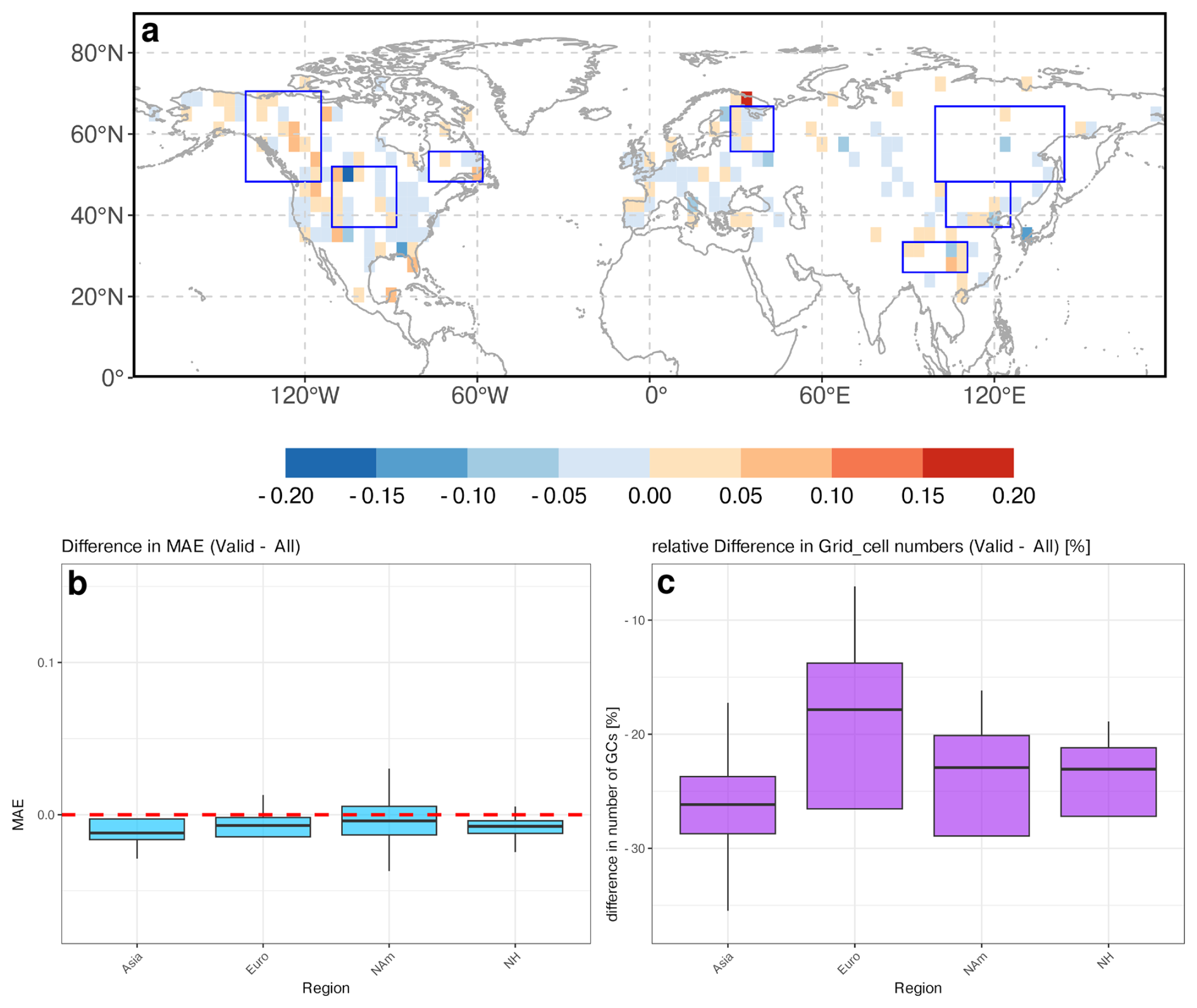
Figure A1(a) Difference in MAE between the simulated and reconstructed tree cover between the comparison with the REVEALS-datasets with only valid grid cells and with all grid cells, (b) mean difference over continents. (c) differences in grid cell number [%] per continent.
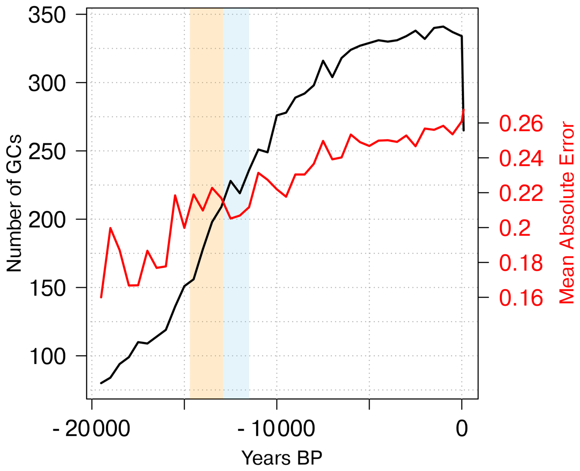
Figure A2MAE between MPI-ESM and REVEALS over time (red) and number of available grid cells per time-steps (black).
In a second set of emulations, we use the emulator trained with the MPI-ESM climate and force it with an idealised, bias-corrected climate, assuming that grid cell specific model biases (e.g. due to differences in the orography) do not change over time (Maraun and Widmann, 2018). We use the delta method following (Beyer et al., 2020) to downscale and bias-correct the simulated climate. For temperature variables, we calculated anomalies between past time-slices and the modern time-slice in the model, bilinearly interpolated these anomalies to a 0.5°-grid and added these to the CRU-TS 4.08 (University of East Anglia Climatic Research Unit et al., 2024; Harris et al., 2020) derived temperature for the period 1931 to 1970. To bias-correct the precipitation, we applied the delta method in a multiplicative way, which is seen to be more appropriate for moisture changes as precipitation covers different orders of magnitudes, depending on the region (Beyer et al., 2020; Maraun and Widmann, 2018). This method typically involves calculating relative anomalies by dividing simulated precipitation at each timestep by a reference period, and then scaling these factors by a modern observational baseline. However, in arid regions, this approach can produce unrealistically high precipitation values, when the present-day simulated precipitation is extremely low, resulting in large delta factors when dividing by these small reference values. When these exaggerated anomalies are then applied to modern observational baselines (which may already be low), the resulting scaled precipitation becomes unreasonably inflated. To cope with this, we adopted a modified delta approach, using the simulated climate at 4 ka as the reference period in regions with dry climates. This adjustment provides a more stable denominator and reduces the risk of over-amplifying anomalies in dry regions. To harmonize the results with present-day conditions, and ensure consistency across the dataset, we applied a correction term based on the relative difference between the simulated precipitation at 0 and 4 ka This effectively normalizes the delta factors to present-day conditions while still preserving the benefits of using the 4 ka baseline in dry regions. The final anomalies were then applied to the modern observational dataset to produce bias-adjusted precipitation fields. As the CRUTS4.0.8 data set does not contain a soil moisture field, we just interpolated MPI-ESM soil moisture to the 0.5°-grid, without correcting biases. Time series of Northern Hemisphere mean precipitation, warm- and cold month temperature for both the original and bias-corrected climate, together with the corresponding difference in mean tree cover between the bias-corrected emulation and the original simulation are shown in Fig. B1 in the Appendix B. In addition, spatial maps of the climate variables at the time of maximum change (∼ 12 ka BP), as well as maps of emulated tree cover, simulated tree cover, and their difference for three representative time slices, are provided in Figs. B2 and B3 in the Appendix B.
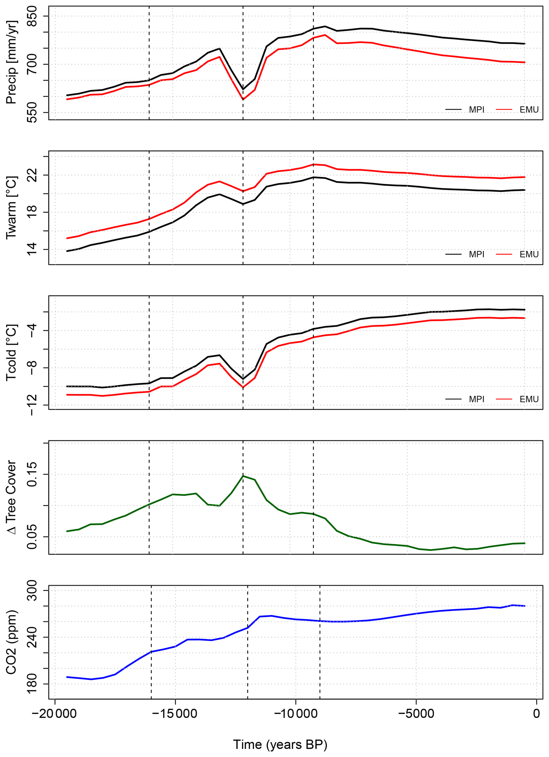
Figure B1Time series of Northern Hemisphere mean precipitation (precip), temperature of the warmest (Twarm) and coldest month (Tcold) for the original (MPI) and bias-corrected (EMU) climate, together with the corresponding difference in mean tree cover between the bias-corrected emulation and the original simulation. Shown is also the global atmospheric CO2 concentration that is used as predictor in the emulation. The dotted lines mark the three time-slices for which maps of tree cover are provided in Fig. B2.
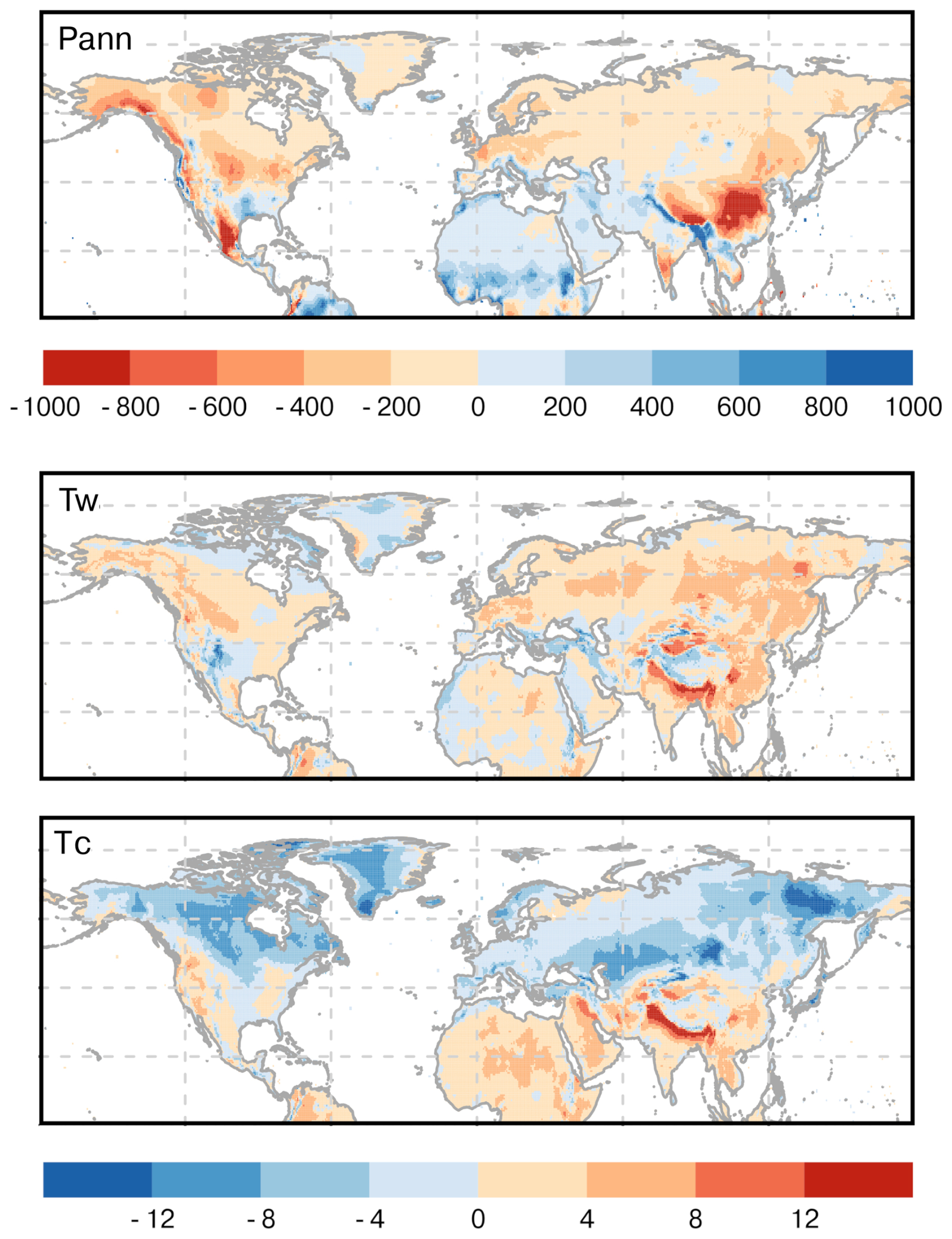
Figure B2Difference in annual mean precipitation (Pann) [mm/year] and in the temperature of the warmest (Tw) and coldest (Tc) month [K] at 12 000 years BP between the bias-corrected and the original simulation. The difference was calculated after remapping the simulation onto a 0.5° grid.
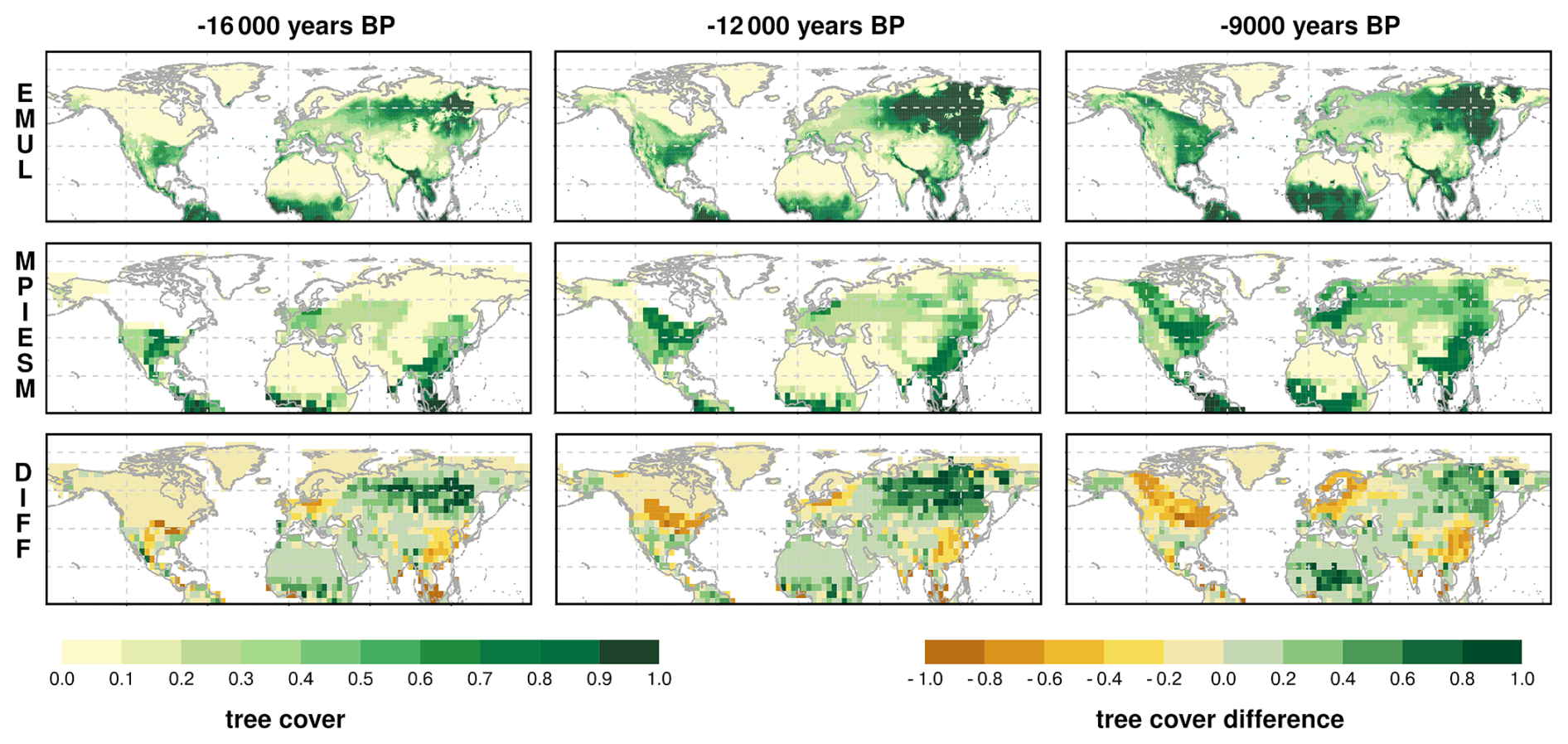
Figure B3Tree cover fraction at different time steps according to the emulation with bias-corrected climate and the MPI-ESM simulation. The bottom panel also shows the difference between the two; for this, the emulation has been remapped to a T31 grid.
To analyse whether the distributions of climate correlations and climate–tree cover dependencies differ among the mae-, r- and var-groups, we used a Kruskal–Wallis test. There results are shown in Figs. C1, C2 and C3. To select important variables for the PCA-analysis, we additionally perform Wilcoxon rank-sum tests to determine variables with significant differences between r-group 1 and 3, mae-group 1 and 4. The results are shown in Table C1.
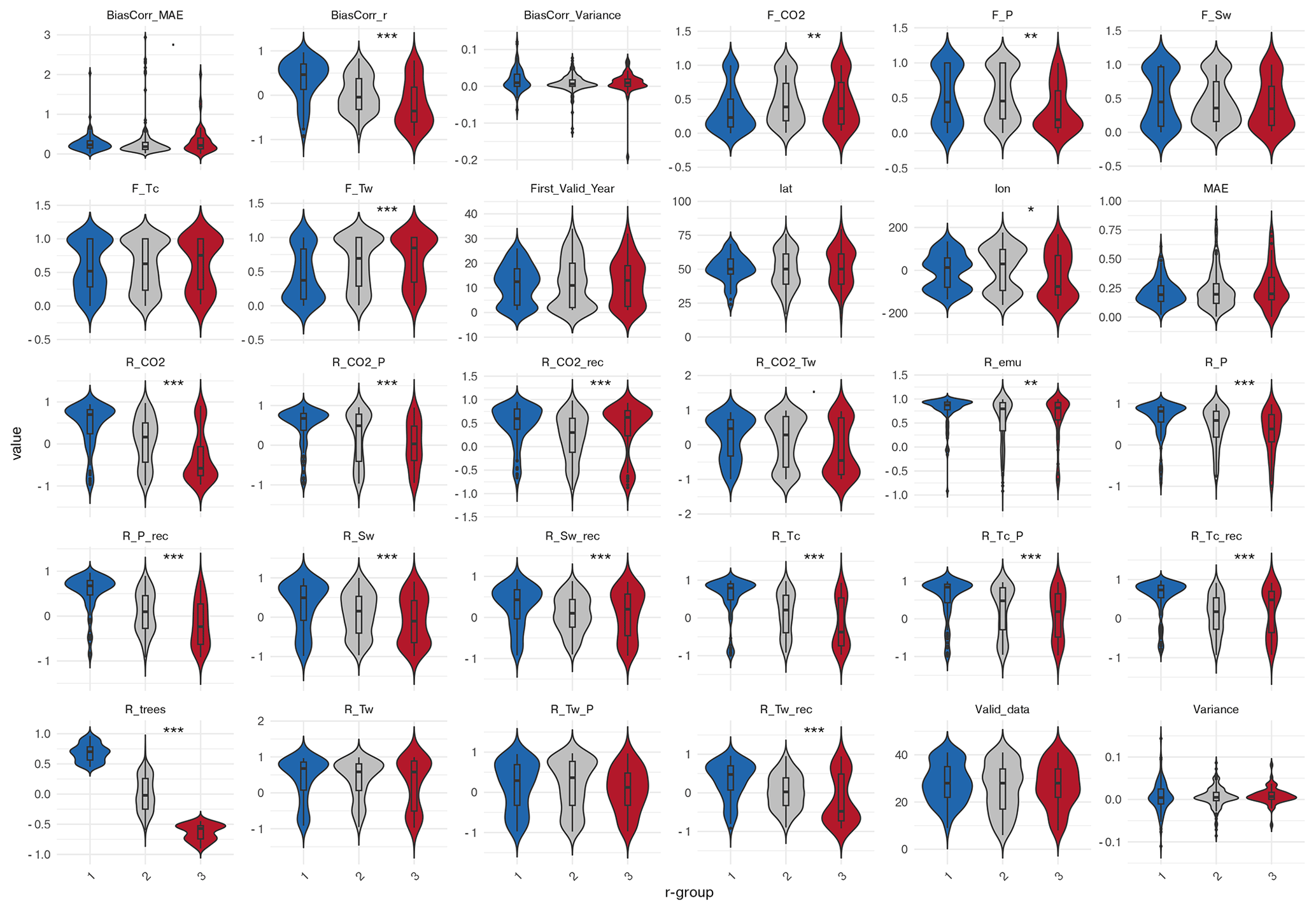
Figure C1Distribution of the coefficients/variables in the different r-groups (1 = positive correlation, 2 = no correlation, 3 = negative correlation) with significance (Kruskal-Wallis, 0.001, 0.01, ∗ 0.05, • 0.1), Hereby, “F_” corresponds to the F-coefficients in the GAM-analysis and “R_” to the Pearson correlation coefficients in the model, or in the reconstructions (“_rec”). The climate variables are Tw: Temperature of the warmest month, Tc: temperature of the coldest month, P: precipitation, Sw: Soil moisture. Valid data describes the number of available time-steps and First_valid_year the first available time-step in the reconstructions. R_Trees is the correlation between the reconstructed and simulated tree cover. “BiasCorr_” denotes the Correlation, MAE and variance differences between the bias-corrected emulation and the reconstructions.
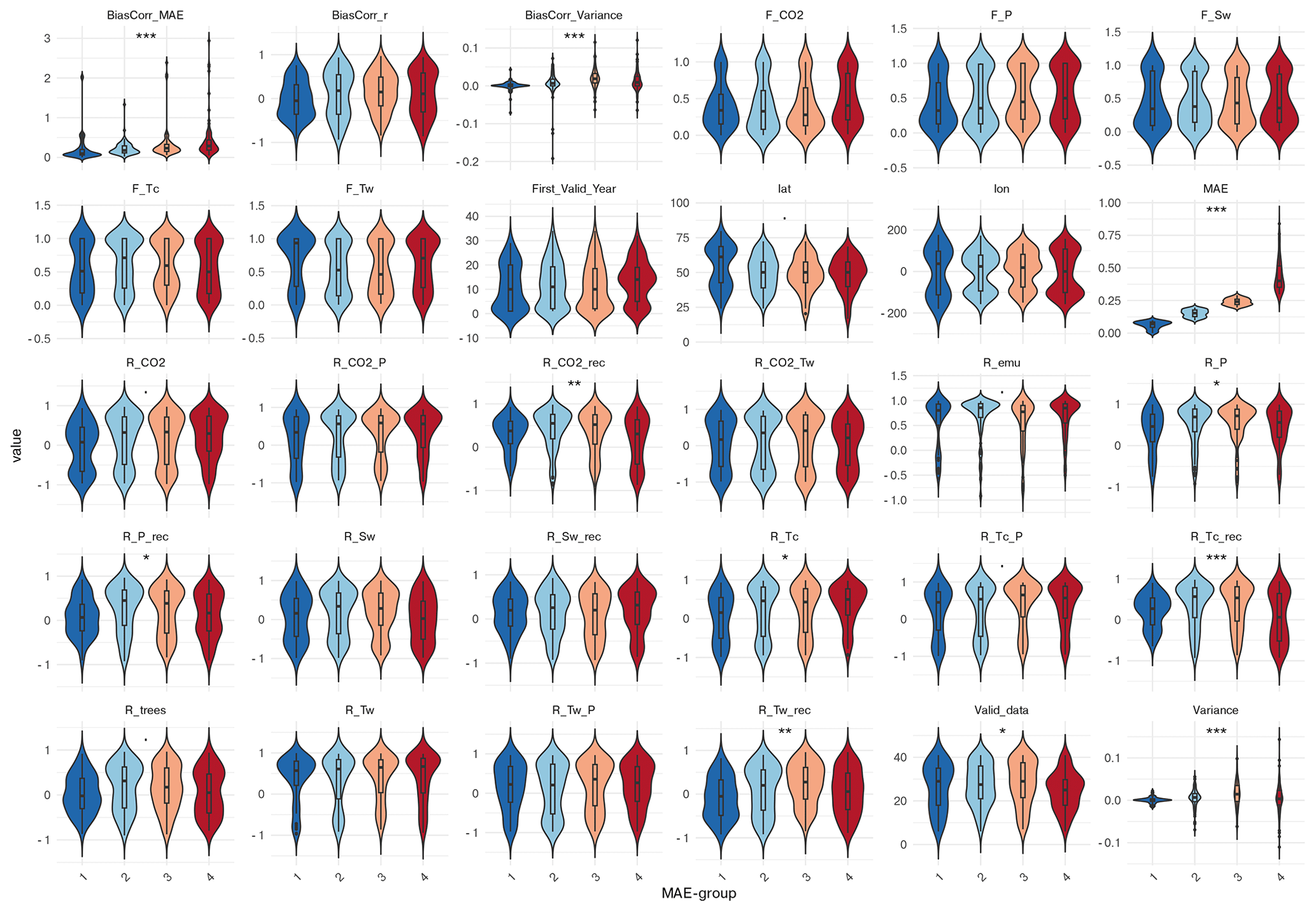
Figure C2Distribution of the coefficients/variables in the different mae-groups (1 = positive correlation, 2 = no correlation, 3 = negative correlation) with significance (Kruskal-Wallis, 0.001, 0.01, ∗ 0.05, • 0.1), Hereby, “F_” corresponds to the F-coefficients in the GAM-analysis and “R_” to the Pearson correlation coefficients in the model, or in the reconstructions (“_rec”). The climate variables are Tw: Temperature of the warmest month, Tc: temperature of the coldest month, P: precipitation, Sw: Soil moisture. Valid data describes the number of available time-steps and First_valid_year the first available time-step in the reconstructions. R_Trees is the correlation between the reconstructed and simulated tree cover. “BiasCorr_” denotes the Correlation, MAE and variance differences between the bias-corrected emulation and the reconstructions.
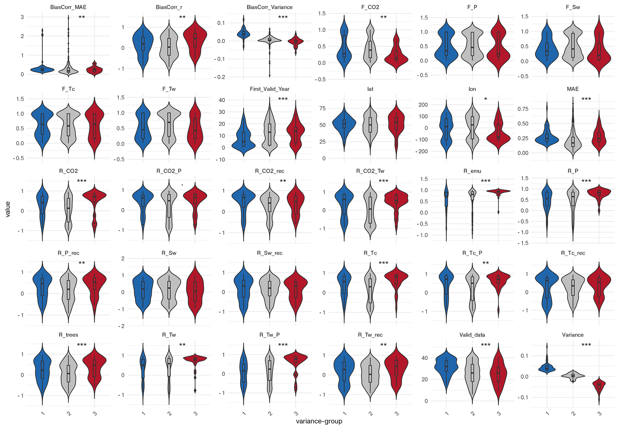
Figure C3Distribution of the coefficients/variables in the different variance-groups (1 = overestimated in MPI-ESM, 2 = similar variance, 3 = underestimated) with significance (Kruskal-Wallis, 0.001, 0.01, ∗ 0.05, • 0.1), Hereby, “F_” corresponds to the F-coefficients in the GAM-analysis and “R_” to the Pearson correlation coefficients in the model, or in the reconstructions (“_rec”). The climate variables are Tw: Temperature of the warmest month, Tc: temperature of the coldest month, P: precipitation, Sw: Soil moisture. Valid data describes the number of available time-steps and First_valid_year the first available time-step in the reconstructions. R_Trees is the correlation between the reconstructed and simulated tree cover. “BiasCorr_” denotes the Correlation, MAE and variance differences between the bias-corrected emulation and the reconstructions.
Table C1Significant difference in the pairwise comparison between the correlation, mae and variance-groups using the Wilcoxon rank-sum test and Kruskal-Wallis test ( 0.001, 0.01, ∗ 0.05, • 0.1, – not significant). Hereby, “F_” corresponds to the F-coefficients in the GAM-analysis representing the non-linear relationship and “R_” to the Pearson correlation coefficients in the model (i.e. linear relationship), or in the reconstructions (“_rec”). The climate variables are Tw: Temperature of the warmest month, Tc: temperature of the coldest month, P: precipitation, and Sw: Soil moisture. Valid data describes the number of available time-steps and First_valid_year the first available time-step in the reconstructions. Lon and lat define the geographical position. R_Trees is the correlation between the reconstructed and simulated tree cover. R_emu is the correlation between the simulated and emulated tree cover.
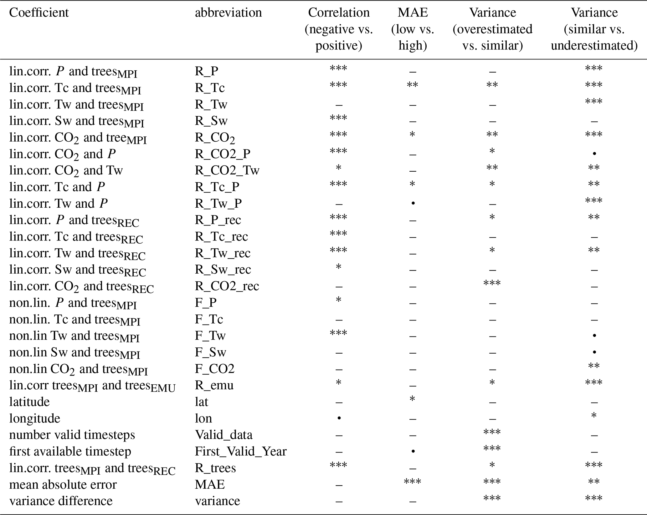
The primary data (i.e. the model source code for MPI-ESM) is freely available to the scientific community upon request to MPI-M. The MPI-ESM model output is available from World Data Center for climate, hosted by the German Climate Computing Center (Deutsches Klimarechenzentrum – DKRZ) at https://doi.org/10.26050/WDCC/PMMXMCHTD (Kleinen et al., 2023b). The REVEALS dataset are freely available from https://doi.org/10.5281/zenodo.17950309 (Schild, 2025). All statistical analyses and visualizations presented in this study were conducted using the R software. Corresponding R scripts and processed datasets are archived here: https://doi.org/10.17617/3.HHMFGX (Dallmeyer and Weitzel, 2026).
A video showing tree cover changes based on MPI-ESM and REVEALS is available at https://doi.org/10.17617/3.O2GGHG (Dallmeyer, 2026).
A.D. and N.W. designed the study. L.S. conducted the pollen-based REVEALS reconstructions and prepared the gridded dataset under the supervision of U.H.; T.K. run the MPI-ESM simulation. N.W. performed the emulations. A.D. carried out the data analysis and wrote the initial draft of the manuscript. All authors contributed to the interpretation of results and to the final version of the manuscript.
At least one of the (co-)authors is a member of the editorial board of Climate of the Past and one of the (co-)authors is a guest member of the editorial board of Climate of the Past for the special issue “Understanding past climate variability to enhance future climate-change projections”. The peer-review process was guided by an independent editor, and the authors also have no other competing interests to declare.
Publisher's note: Copernicus Publications remains neutral with regard to jurisdictional claims made in the text, published maps, institutional affiliations, or any other geographical representation in this paper. The authors bear the ultimate responsibility for providing appropriate place names. Views expressed in the text are those of the authors and do not necessarily reflect the views of the publisher.
This article is part of the special issue “Understanding past climate variability to enhance future climate-change projections (ESD/CP inter-journal SI)”. It is not associated with a conference.
We thank Mateo Duque Villegas for his comments on an earlier version of this manuscript. The authors are grateful to Qiong Zhang and the anonymous reviewer for their constructive and thoughtful comments, which helped to improve the manuscript. We would also like to thank the editor, Bette Otto-Bliesner, for kindly handling this paper. A.D. acknowledges support by the project “HESCOR” funded by the program “Profilbildung 2022”, an initiative of the Ministry of Culture and Science of the State of North-Rhine Westphalia, Germany (HESCOR (grant no. PB22-081)). ChatGPT (OpenAI) was used as a language editing tool to improve grammar, clarity, and readability of the manuscript. All content was subsequently reviewed and validated by the authors.
We gratefully acknowledge the efforts of the Integrated Climate Data Center (ICDC) of CEN at the University of Hamburg for providing MODIS data. This work used resources of the DKRZ, granted by its Scientific Steering Committee (WLA; under project ID bm1030).
This research has been supported by the Bundesministerium für Forschung, Technologie und Raumfahrt (BMFTR) (grant nos. 01LP2306A, 01LP1921A, and 01LP2306B), the Engineering and Physical Sciences Research Council (grant no. EP/Z002591/1), and the European Research Council, H2020 European Research Council (grant no. 951288).
The article processing charges for this open-access publication were covered by the Max Planck Society.
This paper was edited by Bette L. Otto-Bliesner and reviewed by Qiong Zhang and one anonymous referee.
Adam, M., Weitzel, N., and Rehfeld, K.: Identifying Global-Scale Patterns of Vegetation Change During the Last Deglaciation From Paleoclimate Networks, Palaeogeogr. Palaeocl., 36, e2021PA004265, https://doi.org/10.1029/2021PA004265, 2021.
Allen, J. R. M., Forrest, M., Hickler, T., Singarayer, J. S., Valdes, P. J., and Huntley, B.: Global vegetation patterns of the past 140,000 years, J. Biogeogr., 47, 2073–2090, https://doi.org/10.1111/jbi.13930, 2020.
Anhuf, D., Ledru, M.-P., Behling, H., Da Cruz, F. W., Cordeiro, R. C., Van der Hammen, T., Karmann, I., Marengo, J. A., De Oliveira, P. E., Pessenda, L., Siffedine, A., Albuquerque, A. L., and Da Silva Dias, P. L.: Paleo-environmental change in Amazonian and African rainforest during the LGM, Palaeogeogr. Palaeocl., 239, 510–527, https://doi.org/10.1016/j.palaeo.2006.01.017, 2006.
Annan, J. D., Hargreaves, J. C., and Mauritsen, T.: A new global surface temperature reconstruction for the Last Glacial Maximum, Clim. Past, 18, 1883–1896, https://doi.org/10.5194/cp-18-1883-2022, 2022.
Arora, V. K., Katavouta, A., Williams, R. G., Jones, C. D., Brovkin, V., Friedlingstein, P., Schwinger, J., Bopp, L., Boucher, O., Cadule, P., Chamberlain, M. A., Christian, J. R., Delire, C., Fisher, R. A., Hajima, T., Ilyina, T., Joetzjer, E., Kawamiya, M., Koven, C. D., Krasting, J. P., Law, R. M., Lawrence, D. M., Lenton, A., Lindsay, K., Pongratz, J., Raddatz, T., Séférian, R., Tachiiri, K., Tjiputra, J. F., Wiltshire, A., Wu, T., and Ziehn, T.: Carbon–concentration and carbon–climate feedbacks in CMIP6 models and their comparison to CMIP5 models, Biogeosciences, 17, 4173–4222, https://doi.org/10.5194/bg-17-4173-2020, 2020.
Bartlein, P. J., Harrison, S. P., Brewer, S., Connor, S., Davis, B. A. S., Gajewski, K., Guiot, J., Harrison-Prentice, T. I., Henderson, A., Peyron, O., Prentice, I. C., Scholze, M., Seppa, H., Shuman, B., Sugita, S., Thompson, R. S., Viau, A. E., Williams, J., and Wu, H.: Pollen-based continental climate reconstructions at 6 and 21 ka: a global synthesis, Clim. Dynam., 37, 775–802, https://doi.org/10.1007/s00382-010-0904-1, 2011.
Batchelor, C. L., Margold, M., Krapp, M., Murton, D. K., Dalton, A. S., Gibbard, P. L., Stokes, C. R., Murton, J. B., and Manica, A.: The configuration of Northern Hemisphere ice sheets through the Quaternary, Nat. Commun., 10, 3713, https://doi.org/10.1038/s41467-019-11601-2, 2019.
Berger, A. L.: Long-term variations of daily insolation and Quaternary climatic changes, Journal of Atmospheric Sciences, 35, 2361–2367, https://doi.org/10.1175/1520-0469(1978)035<2362:LTVODI>2.0.CO;2, 1978.
Beyer, R., Krapp, M., and Manica, A.: An empirical evaluation of bias correction methods for palaeoclimate simulations, Clim. Past, 16, 1493–1508, https://doi.org/10.5194/cp-16-1493-2020, 2020.
Bigelow, N. H., Brubaker, L. B., Edwards, M. E., Harrison, S. P., Prentice, I. C., Anderson, P. M., Andreev, A. A., Bartlein, P. J., Christensen, T. R., Cramer, W., Kaplan, J. O., Lozhkin, A. V., Matveyeva, N. V., Murray, D. F., McGuire, A. D., Razzhivin, V. Y., Ritchie, J. C., Smith, B., Walker, D. A., Gajewski, K., Wolf, V., Holmqvist, B. H., Igarashi, Y., Kremenetskii, K., Paus, A., Pisaric, M. F. J., and Volkova, V. S.: Climate change and Arctic ecosystems: 1. Vegetation changes north of 55° N between the last glacial maximum, mid-Holocene, and present, J. Geophys. Res.-Atmos., 108, https://doi.org/10.1029/2002jd002558, 2003.
Binney, H., Edwards, M., Macias-Fauria, M., Lozhkin, A., Anderson, P., Kaplan, J. O., Andreev, A., Bezrukova, E., Blyakharchuk, T., Jankovska, V., Khazina, I., Krivonogov, S., Kremenetski, K., Nield, J., Novenko, E., Ryabogina, N., Solovieva, N., Willis, K., and Zernitskaya, V.: Vegetation of Eurasia from the last glacial maximum to present: Key biogeographic patterns, Quaternary Sci. Rev., 157, 80–97, https://doi.org/10.1016/j.quascirev.2016.11.022, 2017.
Braconnot, P., Harrison, S. P., Kageyama, M., Bartlein, P. J., Masson-Delmotte, V., Abe-Ouchi, A., Otto-Bliesner, B., and Zhao, Y.: Evaluation of climate models using palaeoclimatic data, Nat. Clim. Change, 2, 417–424, https://doi.org/10.1038/NCLIMATE1456, 2012.
Cao, X., Tian, F., Li, F., Gaillard, M.-J., Rudaya, N., Xu, Q., and Herzschuh, U.: Pollen-based quantitative land-cover reconstruction for northern Asia covering the last 40 ka cal BP, Clim. Past, 15, 1503–1536, https://doi.org/10.5194/cp-15-1503-2019, 2019a.
Cao, X., Tian, F., Li, F., Gaillard, M.-J., Rudaya, N., Xu, Q., and Herzschuh, U.: Pollen-based quantitative land-cover reconstruction for northern Asia covering the last 40 ka cal BP, Clim. Past, 15, 1503–1536, https://doi.org/10.5194/cp-15-1503-2019, 2019b.
Charrier, G., Nolf, M., Leitinger, G., Charra-Vaskou, K., Losso, A., Tappeiner, U., Améglio, T., and Mayr, S.: Monitoring of Freezing Dynamics in Trees: A Simple Phase Shift Causes Complexity, Plant Physiol., 173, 2196–2207, https://doi.org/10.1104/pp.16.01815, 2017.
Cheng, J., Wu, H., Liu, Z., Gu, P., Wang, J., Zhao, C., Li, Q., Chen, H., Lu, H., Hu, H., Gao, Y., Yu, M., and Song, Y.: Vegetation feedback causes delayed ecosystem response to East Asian Summer Monsoon Rainfall during the Holocene, Nat. Commun., 12, 1–9, https://doi.org/10.1038/s41467-021-22087-2, 2021.
Clark, P. U., Shakun, J. D., Baker, P. A., Bartlein, P. J., Brewer, S., Brook, E., Carlson, A. E., Cheng, H., Kaufman, D. S., Liu, Z., Marchitto, T. M., Mix, A. C., Morrill, C., Otto-Bliesner, B. L., Pahnke, K., Russell, J. M., Whitlock, C., Adkins, J. F., Blois, J. L., Clark, J., Colman, S. M., Curry, W. B., Flower, B. P., He, F., Johnson, T. C., Lynch-Stieglitz, J., Markgraf, V., McManus, J., Mitrovica, J. X., Moreno, P. I., and Williams, J. W.: Global climate evolution during the last deglaciation, P. Natl. Acad. Sci. USA, 109, E1134–E1142, https://doi.org/10.1073/pnas.1116619109, 2012.
Claussen, M., Selent, K., Brovkin, V., Raddatz, T., and Gayler, V.: Impact of CO2 and climate on Last Glacial maximum vegetation – a factor separation, Biogeosciences, 10, 3593–3604, https://doi.org/10.5194/bg-10-3593-2013, 2013.
Dallmeyer, A.: From Ice Age to Present: Tree Cover Dynamics in REVEALS and MPI-ESM (Video), Edmond, V1 [video], https://doi.org/10.17617/3.O2GGHG, 2026.
Dallmeyer, A. and Weitzel, N.: Processed Data and Scripts for “Unravelling the Tree Cover Dynamics over the Last 20,000 Years on the Northern Hemisphere”, Edmond [data set], https://doi.org/10.17617/3.HHMFGX, 2026.
Dallmeyer, A., Claussen, M., and Brovkin, V.: Harmonising plant functional type distributions for evaluating Earth system models, Clim. Past, 15, 335–366, https://doi.org/10.5194/cp-15-335-2019, 2019.
Dallmeyer, A., Claussen, M., Lorenz, S. J., Sigl, M., Toohey, M., and Herzschuh, U.: Holocene vegetation transitions and their climatic drivers in MPI-ESM1.2, Clim. Past, 17, 2481–2513, https://doi.org/10.5194/cp-17-2481-2021, 2021.
Dallmeyer, A., Kleinen, T., Claussen, M., Weitzel, N., Cao, X., and Herzschuh, U.: The deglacial forest conundrum, Nat. Commun., 13, 6035, https://doi.org/10.1038/s41467-022-33646-6, 2022.
Dallmeyer, A., Poska, A., Marquer, L., Seim, A., and Gaillard, M.-J.: The challenge of comparing pollen-based quantitative vegetation reconstructions with outputs from vegetation models – a European perspective, Clim. Past, 19, 1531–1557, https://doi.org/10.5194/cp-19-1531-2023, 2023.
Davis, B. A. S., Fasel, M., Kaplan, J. O., Russo, E., and Burke, A.: The climate and vegetation of Europe, northern Africa, and the Middle East during the Last Glacial Maximum (21 000 yr BP) based on pollen data, Clim. Past, 20, 1939–1988, https://doi.org/10.5194/cp-20-1939-2024, 2024.
Dawson, A., Williams, J. W., Gaillard, M.-J., Goring, S. J., Pirzamanbein, B., Lindstrom, J., Anderson, R. S., Brunelle, A., Foster, D., Gajewski, K., Gavin, D. G., Lacourse, T., Minckley, T. A., Oswald, W., Shuman, B., and Whitlock, C.: Holocene land cover change in North America: continental trends, regional drivers, and implications for vegetation–atmosphere feedbacks, Clim. Past, 21, 2031–2060, https://doi.org/10.5194/cp-21-2031-2025, 2025.
DiMiceli, D., Sohlberg, R., and Townshend, J.: MODIS/Terra Vegetation Continuous Fields Yearly L3 Global 250m SIN Grid V061, NASA Land Processes Distributed Active Archive Center [data set], https://doi.org/10.5067/MODIS/MOD44B.061, 2022.
Dupont, L. M., Jahns, S., Marret, F., and Ning, S.: Vegetation change in equatorial West Africa: time-slices for the last 150 ka, Palaeogeogr. Palaeocl., 155, 95–122, https://doi.org/10.1016/S0031-0182(99)00095-4, 2000.
Ellis, E. C., Kaplan, J. O., Fuller, D. Q., Vavrus, S., Klein Goldewijk, K., and Verburg, P. H.: Used planet: A global history, P. Natl. Acad. Sci. USA, 110, 7978–7985, https://doi.org/10.1073/pnas.1217241110, 2013.
Fyfe, R. M., de Beaulieu, J.-L., Binney, H., Bradshaw, R. H. W., Brewer, S., Le Flao, A., Finsinger, W., Gaillard, M.-J., Giesecke, T., Gil-Romera, G., Grimm, E. C., Huntley, B., Kunes, P., Kühl, N., Leydet, M., Lotter, A. F., Tarasov, P. E., and Tonkov, S.: The European Pollen Database: past efforts and current activities, Veg. Hist. Archaeobot., 18, 417–424, https://doi.org/10.1007/s00334-009-0215-9, 2009.
Gaillard, M.-J., Sugita, S., Mazier, F., Trondman, A.-K., Broström, A., Hickler, T., Kaplan, J. O., Kjellström, E., Kokfelt, U., Kuneš, P., Lemmen, C., Miller, P., Olofsson, J., Poska, A., Rundgren, M., Smith, B., Strandberg, G., Fyfe, R., Nielsen, A. B., Alenius, T., Balakauskas, L., Barnekow, L., Birks, H. J. B., Bjune, A., Björkman, L., Giesecke, T., Hjelle, K., Kalnina, L., Kangur, M., van der Knaap, W. O., Koff, T., Lagerås, P., Latałowa, M., Leydet, M., Lechterbeck, J., Lindbladh, M., Odgaard, B., Peglar, S., Segerström, U., von Stedingk, H., and Seppä, H.: Holocene land-cover reconstructions for studies on land cover-climate feedbacks, Clim. Past, 6, 483–499, https://doi.org/10.5194/cp-6-483-2010, 2010.
Giesecke, T., Ammann, B., and Brande, A.: Palynological richness and evenness: insights from the taxa accumulation curve, Veg. Hist. Archaeobot., 23, 217–228, https://doi.org/10.1007/s00334-014-0435-5, 2014.
Githumbi, E., Fyfe, R., Gaillard, M.-J., Trondman, A.-K., Mazier, F., Nielsen, A.-B., Poska, A., Sugita, S., Woodbridge, J., Azuara, J., Feurdean, A., Grindean, R., Lebreton, V., Marquer, L., Nebout-Combourieu, N., Stančikaitė, M., Tanţău, I., Tonkov, S., Shumilovskikh, L., and LandClimII data contributors: European pollen-based REVEALS land-cover reconstructions for the Holocene: methodology, mapping and potentials, Earth Syst. Sci. Data, 14, 1581–1619, https://doi.org/10.5194/essd-14-1581-2022, 2022.
Gosling, W. D., Miller, C. S., Shanahan, T. M., Holden, P. B., Overpeck, J. T., and van Langevelde, F.: A stronger role for long-term moisture change than for CO2 in determining tropical woody vegetation change, Science, 376, 653–656, https://doi.org/10.1126/science.abg4618, 2022.
Hao, S., Zhang, X., Duan, Y., Gowan, E. J., Zhu, J., Cauquoin, A., Chen, J., Werner, M., and Chen, F.: Model seasonal and proxy spatial biases revealed by assimilated mid-Holocene seasonal temperatures, Sci. Bull., 70, 2014–2022, https://doi.org/10.1016/j.scib.2025.03.039, 2025.
Harris, I., Osborn, T. J., Jones, P., and Lister, D.: Version 4 of the CRU TS monthly high-resolution gridded multivariate climate dataset, Scientific Data, 7, 109, https://doi.org/10.1038/s41597-020-0453-3, 2020.
Harrison, S. P., Bartlein, P. J., Izumi, K., Li, G., Annan, J., Hargreaves, J., Braconnot, P., and Kageyama, M.: Evaluation of CMIP5 palaeo-simulations to improve climate projections, Nat. Clim. Change, 5, 735–743, https://doi.org/10.1038/nclimate2649, 2015.
Helbig, M., Pappas, C., and Sonnentag, O.: Permafrost thaw and wildfire: Equally important drivers of boreal tree cover changes in the Taiga Plains, Canada, Geophys. Res. Lett., 43, 1598–1606, https://doi.org/10.1002/2015GL067193, 2016.
Herzschuh, U., Birks, H. J. B., Laepple, T., Andreev, A., Melles, M., and Brigham-Grette, J.: Glacial legacies on interglacial vegetation at the Pliocene-Pleistocene transition in NE Asia, Nat. Commun., 7, 1–11, https://doi.org/10.1038/ncomms11967, 2016.
Herzschuh, U., Li, C., Böhmer, T., Postl, A. K., Heim, B., Andreev, A. A., Cao, X., Wieczorek, M., and Ni, J.: LegacyPollen 1.0: a taxonomically harmonized global late Quaternary pollen dataset of 2831 records with standardized chronologies, Earth Syst. Sci. Data, 14, 3213–3227, https://doi.org/10.5194/essd-14-3213-2022, 2022.
Horvath, P., Tang, H., Halvorsen, R., Stordal, F., Tallaksen, L. M., Berntsen, T. K., and Bryn, A.: Improving the representation of high-latitude vegetation distribution in dynamic global vegetation models, Biogeosciences, 18, 95–112, https://doi.org/10.5194/bg-18-95-2021, 2021.
Ivanovic, R. F., Gregoire, L. J., Kageyama, M., Roche, D. M., Valdes, P. J., Burke, A., Drummond, R., Peltier, W. R., and Tarasov, L.: Transient climate simulations of the deglaciation 21–9 thousand years before present (version 1) – PMIP4 Core experiment design and boundary conditions, Geosci. Model Dev., 9, 2563–2587, https://doi.org/10.5194/gmd-9-2563-2016, 2016.
Jin, H., Huang, Y., Bense, V. F., Ma, Q., Marchenko, S. S., Shepelev, V. V., Hu, Y., Liang, S., Spektor, V. V., Jin, X., Li, X., and Li, X.: Permafrost Degradation and Its Hydrogeological Impacts, Water, 14, 372, https://doi.org/10.3390/w14030372, 2022.
Jin, X.-Y., Jin, H.-J., Iwahana, G., Marchenko, S. S., Luo, D.-L., Li, X.-Y., and Liang, S.-H.: Impacts of climate-induced permafrost degradation on vegetation: A review, Advances in Climate Change Research, 12, 29–47, https://doi.org/10.1016/j.accre.2020.07.002, 2021.
Kaplan, J. O., Krumhardt, K. M., Ellis, E. C., Ruddiman, W. F., Lemmen, C., and Goldewijk, K. K.: Holocene carbon emissions as a result of anthropogenic land cover change, The Holocene, 21, 775–791, https://doi.org/10.1177/0959683610386983, 2011.
Kaplan, J. O., Krumhardt, K. M., Gaillard, M.-J., Sugita, S., Trondman, A.-K., Fyfe, R., Marquer, L., Mazier, F., and Nielsen, A. B.: Constraining the Deforestation History of Europe: Evaluation of Historical Land Use Scenarios with Pollen-Based Land Cover Reconstructions, Land, 6, 91, https://doi.org/10.3390/land6040091, 2017.
Kern, O. A., Maier, A., and Vercauteren, N.: Landscape reconstructions for Europe during the late Last Glacial (60–20 ka BP): a pollen-based REVEALS approach, Earth Syst. Sci. Data, 17, 5997–6023, https://doi.org/10.5194/essd-17-5997-2025, 2025.
Kim, I.-W., Timmermann, A., Kim, J.-E., Rodgers, K. B., Lee, S.-S., Lee, H., and Wieder, W. R.: Abrupt increase in Arctic-Subarctic wildfires caused by future permafrost thaw, Nat. Commun., 15, 7868, https://doi.org/10.1038/s41467-024-51471-x, 2024.
Kleinen, T., Gromov, S., Steil, B., and Brovkin, V.: Atmospheric methane since the last glacial maximum was driven by wetland sources, Clim. Past, 19, 1081–1099, https://doi.org/10.5194/cp-19-1081-2023, 2023a.
Kleinen, T., Gromov, S., Steil, B., and Brovkin, V.: PalMod2 MPI-M MPI-ESM1-2-CR-CH4 transient-deglaciation-prescribed-glac1d-methane, World Data Center for Climate (WDCC) at DKRZ [data set], https://doi.org/10.26050/WDCC/PMMXMCHTD, 2023b.
Köhler, P., Nehrbass-Ahles, C., Schmitt, J., Stocker, T. F., and Fischer, H.: A 156 kyr smoothed history of the atmospheric greenhouse gases CO2, CH4, and N2O and their radiative forcing, Earth Syst. Sci. Data, 9, 363–387, https://doi.org/10.5194/essd-9-363-2017, 2017.
Kruse, S., Stuenzi, S. M., Boike, J., Langer, M., Gloy, J., and Herzschuh, U.: Novel coupled permafrost–forest model (LAVESI–CryoGrid v1.0) revealing the interplay between permafrost, vegetation, and climate across eastern Siberia, Geosci. Model Dev., 15, 2395–2422, https://doi.org/10.5194/gmd-15-2395-2022, 2022.
Leroy, S. A. G., Arpe, K., Mikolajewicz, U., and Wu, J.: Climate simulations and pollen data reveal the distribution and connectivity of temperate tree populations in eastern Asia during the Last Glacial Maximum, Clim. Past, 16, 2039–2054, https://doi.org/10.5194/cp-16-2039-2020, 2020.
Li, C., Dallmeyer, A., Ni, J., Chevalier, M., Willeit, M., Andreev, A. A., Cao, X., Schild, L., Heim, B., Wieczorek, M., and Herzschuh, U.: Global biome changes over the last 21 000 years inferred from model–data comparisons, Clim. Past, 21, 1001–1024, https://doi.org/10.5194/cp-21-1001-2025, 2025a.
Li, C., Ni, J., Böhmer, T., Cao, X., Zhou, B., Liao, M., Li, K., Schild, L., Wieczorek, M., Heim, B., and Herzschuh, U.: LegacyPollen2.0: an updated global taxonomically and temporally standardized fossil pollen dataset of 3680 palynological records, PANGAEA [data set], https://doi.org/10.1594/PANGAEA.965907, 2025b.
Li, F., Gaillard, M.-J., Cao, X., Herzschuh, U., Sugita, S., Ni, J., Zhao, Y., An, C., Huang, X., Li, Y., Liu, H., Sun, A., and Yao, Y.: Gridded pollen-based Holocene regional plant cover in temperate and northern subtropical China suitable for climate modelling, Earth Syst. Sci. Data, 15, 95–112, https://doi.org/10.5194/essd-15-95-2023, 2023a.
Li, F., Gaillard, M.-J., Cao, X., Herzschuh, U., Sugita, S., Ni, J., Zhao, Y., An, C., Huang, X., Li, Y., Liu, H., Sun, A., and Yao, Y.: Gridded pollen-based Holocene regional plant cover in temperate and northern subtropical China suitable for climate modelling, Earth Syst. Sci. Data, 15, 95–112, https://doi.org/10.5194/essd-15-95-2023, 2023b.
Li, G., Chen, W., Zhang, X., Yang, Z., Wang, Z., and Bi, P.: Spatiotemporal changes and driving factors of vegetation in 14 different climatic regions in the global from 1981 to 2018, Environ. Sci. Pollut. Res., 29, 75322–75337, https://doi.org/10.1007/s11356-022-21138-5, 2022a.
Li, W., Tian, F., Rudaya, N., Herzschuh, U., and Cao, X.: Pollen-Based Holocene Thawing-History of Permafrost in Northern Asia and Its Potential Impacts on Climate Change, Front. Ecol. Evol., 10, https://doi.org/10.3389/fevo.2022.894471, 2022b.
MacDonald, G. M., Velichko, A. A., Kremenetski, C. V., Borisova, O. K., Goleva, A. A., Andreev, A. A., Cwynar, L. C., Riding, R. T., Forman, S. L., Edwards, T. W. D., Aravena, R., Hammarlund, D., Szeicz, J. M., and Gattaulin, V. N.: Holocene Treeline History and Climate Change Across Northern Eurasia, Quaternary Res., 53, 302–311, https://doi.org/10.1006/qres.1999.2123, 2000.
Maraun, D. and Widmann, M.: Statistical Downscaling and Bias Correction for Climate Research, 1st Edn., Cambridge University Press, https://doi.org/10.1017/9781107588783, 2018.
Marquer, L., Gaillard, M.-J., Sugita, S., Poska, A., Trondman, A.-K., Mazier, F., Nielsen, A. B., Fyfe, R. M., Jönsson, A. M., Smith, B., Kaplan, J. O., Alenius, T., Birks, H. J. B., Bjune, A. E., Christiansen, J., Dodson, J., Edwards, K. J., Giesecke, T., Herzschuh, U., Kangur, M., Koff, T., Latałowa, M., Lechterbeck, J., Olofsson, J., and Seppä, H.: Quantifying the effects of land use and climate on Holocene vegetation in Europe, Quaternary Sci. Rev., 171, 20–37, https://doi.org/10.1016/j.quascirev.2017.07.001, 2017.
Mauritsen, T., Bader, J., Becker, T., Behrens, J., Bittner, M., Brokopf, R., Brovkin, V., Claussen, M., Crueger, T., Esch, M., Fast, I., Fiedler, S., Fläschner, D., Gayler, V., Giorgetta, M., Goll, D. S., Haak, H., Hagemann, S., Hedemann, C., Hohenegger, C., Ilyina, T., Jahns, T., Jimenéz-de-la-Cuesta, D., Jungclaus, J., Kleinen, T., Kloster, S., Kracher, D., Kinne, S., Kleberg, D., Lasslop, G., Kornblueh, L., Marotzke, J., Matei, D., Meraner, K., Mikolajewicz, U., Modali, K., Möbis, B., Müller, W. A., Nabel, J. E. M. S., Nam, C. C. W., Notz, D., Nyawira, S., Paulsen, H., Peters, K., Pincus, R., Pohlmann, H., Pongratz, J., Popp, M., Raddatz, T. J., Rast, S., Redler, R., Reick, C. H., Rohrschneider, T., Schemann, V., Schmidt, H., Schnur, R., Schulzweida, U., Six, K. D., Stein, L., Stemmler, I., Stevens, B., Storch, J., Tian, F., Voigt, A., Vrese, P., Wieners, K., Wilkenskjeld, S., Winkler, A., and Roeckner, E.: Developments in the MPI-M Earth System Model version 1.2 (MPI-ESM1.2) and Its Response to Increasing CO 2, J. Adv. Model. Earth Syst., 11, 998–1038, https://doi.org/10.1029/2018MS001400, 2019.
McGee, D.: Glacial–Interglacial Precipitation Changes, Annu. Rev. Mar. Sci., 12, 525–557, https://doi.org/10.1146/annurev-marine-010419-010859, 2020.
Montesano, P. M., Nelson, R., Sun, G., Margolis, H., Kerber, A., and Ranson, K. J.: MODIS tree cover validation for the circumpolar taiga–tundra transition zone, Remote Sens. Environ., 113, 2130–2141, https://doi.org/10.1016/j.rse.2009.05.021, 2009.
Mottl, O., Flantua, S. G. A., Bhatta, K. P., Felde, V. A., Giesecke, T., Goring, S., Grimm, E. C., Haberle, S., Hooghiemstra, H., Ivory, S., Kuneš, P., Wolters, S., Seddon, A. W. R., and Williams, J. W.: Global acceleration in rates of vegetation change over the past 18,000 years, Science, 372, 860–864, https://doi.org/10.1126/science.abg1685, 2021.
Nolan, C., Overpeck, J. T., Allen, J. R. M., Anderson, P. M., Betancourt, J. L., Binney, H. A., Brewer, S., Bush, M. B., Chase, B. M., Cheddadi, R., Djamali, M., Dodson, J., Edwards, M. E., Gosling, W. D., Haberle, S., Hotchkiss, S. C., Huntley, B., Ivory, S. J., Kershaw, A. P., Kim, S. H., Latorre, C., Leydet, M., Lézine, A. M., Liu, K. B., Liu, Y., Lozhkin, A. V., McGlone, M. S., Marchant, R. A., Momohara, A., Moreno, P. I., Müller, S., Otto-Bliesner, B. L., Shen, C., Stevenson, J., Takahara, H., Tarasov, P. E., Tipton, J., Vincens, A., Weng, C., Xu, Q., Zheng, Z., and Jackson, S. T.: Past and future global transformation of terrestrial ecosystems under climate change, Science, 361, 920–923, https://doi.org/10.1126/science.aan5360, 2018.
Osman, M. B., Tierney, J. E., Zhu, J., Tardif, R., Hakim, G. J., King, J., and Poulsen, C. J.: Globally resolved surface temperatures since the Last Glacial Maximum, Nature, 599, 239–244, https://doi.org/10.1038/s41586-021-03984-4, 2021.
Prentice, I. C., Jolly, D., and BIOME 6000 participants: Mid-Holocene and glacial-maximum vegetation geography of the northern continents and Africa, J. Biogeogr., 27, 507–519, https://doi.org/10.1046/j.1365-2699.2000.00425.x, 2000.
Reick, C. H., Raddatz, T., Brovkin, V., and Gayler, V.: Representation of natural and anthropogenic land cover change in MPI-ESM, J. Adv. Model. Earth Syst., 5, 459–482, https://doi.org/10.1002/jame.20022, 2013.
Reick, C. H., Gayler, V., Goll, D., Hagemann, S., Heidkamp, M., Nabel, J. E. M. S., Raddatz, T., Roeckner, E., Schnur, R., and Wilkenskjeld, S.: JSBACH 3 – The land component of the MPI Earth System Model: documentation of version 3.2, Berichte zur Erdsystemforschung, 240, https://doi.org/10.17617/2.3279802, 2021.
Roberts, N., Fyfe, R. M., Woodbridge, J., Gaillard, M.-J., Davis, B. A. S., Kaplan, J. O., Marquer, L., Mazier, F., Nielsen, A. B., Sugita, S., Trondman, A.-K., and Leydet, M.: Europe's lost forests: a pollen-based synthesis for the last 11,000 years, Sci. Rep., 8, 716, https://doi.org/10.1038/s41598-017-18646-7, 2018.
Roebroek, C. T. J., Caporaso, L., Duveiller, G., Davin, E. L., Seneviratne, S. I., and Cescatti, A.: Potential tree cover under current and future climate scenarios, Scientific Data, 12, 564, https://doi.org/10.1038/s41597-025-04408-y, 2025.
Rogers, A., Medlyn, B. E., Dukes, J. S., Bonan, G., von Caemmerer, S., Dietze, M. C., Kattge, J., Leakey, A. D. B., Mercado, L. M., Niinemets, Ü., Prentice, I. C., Serbin, S. P., Sitch, S., Way, D. A., and Zaehle, S.: A roadmap for improving the representation of photosynthesis in Earth system models, New Phytol., 213, 22–42, https://doi.org/10.1111/nph.14283, 2017.
Sakai, A. and Larcher, W.: Frost Survival of Plants, Springer, Berlin, Heidelberg, https://doi.org/10.1007/978-3-642-71745-1, 1987.
Sato, H., Kelley, D. I., Mayor, S. J., Martin Calvo, M., Cowling, S. A., and Prentice, I. C.: Dry corridors opened by fire and low CO2 in Amazonian rainforest during the Last Glacial Maximum, Nat. Geosci., 14, 578–585, https://doi.org/10.1038/s41561-021-00777-2, 2021.
Schild, L.: Northern Hemisphere REVEALS-based forest cover for the past 20 k years, Zenodo [data set], https://doi.org/10.5281/zenodo.17950309, 2025.
Schild, L., Ewald, P., Li, C., Hébert, R., Laepple, T., and Herzschuh, U.: LegacyVegetation: Northern Hemisphere reconstruction of past plant cover and total tree cover from pollen archives of the last 14 kyr, Earth Syst. Sci. Data, 17, 2007–2033, https://doi.org/10.5194/essd-17-2007-2025, 2025.
Seddon, A. W. R., Macias-Fauria, M., Long, P. R., Benz, D., and Willis, K. J.: Sensitivity of global terrestrial ecosystems to climate variability, Nature, 531, 229–232, https://doi.org/10.1038/nature16986, 2016.
Shakun, J. D., Clark, P. U., He, F., Marcott, S. A., Mix, A. C., Liu, Z., Otto-Bliesner, B., Schmittner, A., and Bard, E.: Global warming preceded by increasing carbon dioxide concentrations during the last deglaciation, Nature, 484, 49–54, https://doi.org/10.1038/nature10915, 2012.
Shi, X., Werner, M., Yang, H., D'Agostino, R., Liu, J., Yang, C., and Lohmann, G.: Unraveling the complexities of the Last Glacial Maximum climate: the role of individual boundary conditions and forcings, Clim. Past, 19, 2157–2175, https://doi.org/10.5194/cp-19-2157-2023, 2023.
Stephens, L., Fuller, D., Boivin, N., Rick, T., Gauthier, N., Kay, A., Marwick, B., Armstrong, C. G., Barton, C. M., Denham, T., Douglass, K., Driver, J., Janz, L., Roberts, P., Rogers, J. D., Thakar, H., Altaweel, M., Johnson, A. L., Sampietro Vattuone, M. M., Aldenderfer, M., Archila, S., Artioli, G., Bale, M. T., Beach, T., Borrell, F., Braje, T., Buckland, P. I., Jiménez Cano, N. G., Capriles, J. M., Diez Castillo, A., Çilingiroğlu, Ç., Cleary, M. N., Conolly, J., Coutros, P. R., Covey, R. A., Cremaschi, M., Crowther, A., Der, L., di Lernia, S., Doershuk, J. F., Doolittle, W. E., Edwards, K. J., Erlandson, J. M., Evans, D., Fairbairn, A., Faulkner, P., Feinman, G., Fernandes, R., Fitzpatrick, S. M., Fyfe, R., Garcea, E., Goldstein, S., Goodman, R. C., Guedes, J. D., Herrmann, J., Hiscock, P., Hommel, P., Horsburgh, K. A., Hritz, C., Ives, J. W., Junno, A., Kahn, J. G., Kaufman, B., Kearns, C., Kidder, T. R., Lanoë, F., Lawrence, D., Lee, G.-A., Levin, M. J., Lindskoug, H. B., López-Sáez, J. A., Macrae, S., Marchant, R., Marston, J. M., McClure, S., McCoy, M. D., Ventresca Miller, A., Morrison, M., Motuzaite Matuzeviciute, G., Müller, J., Nayak, A., Noerwidi, S., Peres, T. M., Peterson, C. E., Proctor, L., Randall, A. R., Renette, S., Schug, G. R., Ryzewski, K., Saini, R., Scheinsohn, V., Schmidt, P., Sebillaud, P., Seitsonen, O., Simpson, I. A., Sołtysiak, A., Speakman, R. J., Spengler, R. N., Steffen, M. L., Storozum, M. J., Strickland, K. M., Thompson, J., Thurston, T. L., Ulm, S., Ustunkaya, M. C., Welker, M. H., West, C., Williams, P. R., Wright, D. K., Wright, N., Zahir, M., Zerboni, A., Beaudoin, E., Munevar Garcia, S., Powell, J., Thornton, A., Kaplan, J. O., Gaillard, M.-J., Klein Goldewijk, K., and Ellis, E.: Archaeological assessment reveals Earth's early transformation through land use, Science, 365, 897–902, https://doi.org/10.1126/science.aax1192, 2019.
Stuenzi, S. M., Boike, J., Gädeke, A., Herzschuh, U., Kruse, S., Pestryakova, L. A., Westermann, S., and Langer, M.: Sensitivity of ecosystem-protected permafrost under changing boreal forest structures, Environ. Res. Lett., 16, 084045, https://doi.org/10.1088/1748-9326/ac153d, 2021.
Sugita, S.: Theory of quantitative reconstruction of vegetation I: pollen from large sites REVEALS regional vegetation composition, The Holocene, 17, 229–241, https://doi.org/10.1177/0959683607075837, 2007.
Sweeney, L., Harrison, S. P., and Vander Linden, M.: European tree cover during the Holocene reconstructed from pollen records, Biogeosciences, 22, 4903–4922, https://doi.org/10.5194/bg-22-4903-2025, 2025.
Tarasov, L., Dyke, A. S., Neal, R. M., and Peltier, W. R.: A data-calibrated distribution of deglacial chronologies for the North American ice complex from glaciological modeling, Earth Planet. Sc. Lett., 315–316, 30–40, https://doi.org/10.1016/j.epsl.2011.09.010, 2012.
Theuerkauf, M., Couwenberg, J., Kuparinen, A., and Liebscher, V.: A matter of dispersal: REVEALSinR introduces state-of-the-art dispersal models to quantitative vegetation reconstruction, Veg. Hist. Archaeobot., 25, 541–553, https://doi.org/10.1007/s00334-016-0572-0, 2016.
Thompson, A. J., Zhu, J., Poulsen, C. J., Tierney, J. E., and Skinner, C. B.: Northern Hemisphere vegetation change drives a Holocene thermal maximum, Science Advances, 8, eabj6535, https://doi.org/10.1126/sciadv.abj6535, 2022.
Tian, F., Cao, X., Dallmeyer, A., Lohmann, G., Zhang, X., Ni, J., Andreev, A., Anderson, P. M., Lozhkin, A. V., Bezrukova, E., Rudaya, N., Xu, Q., and Herzschuh, U.: Biome changes and their inferred climatic drivers in northern and eastern continental Asia at selected times since 40 cal ka bp, Veg. Hist. Archaeobot., 27, 365–379, https://doi.org/10.1007/s00334-017-0653-8, 2018.
Tian, Z. and Jiang, D.: Mid-Holocene ocean and vegetation feedbacks over East Asia, Clim. Past, 9, 2153–2171, https://doi.org/10.5194/cp-9-2153-2013, 2013.
Tierney, J. E., Zhu, J., King, J., Malevich, S. B., Hakim, G. J., and Poulsen, C. J.: Glacial cooling and climate sensitivity revisited, Nature, 584, 569, https://doi.org/10.1038/s41586-020-2617-x, 2020.
Trondman, A. -K., Gaillard, M. -J., Mazier, F., Sugita, S., Fyfe, R., Nielsen, A. B., Twiddle, C., Barratt, P., Birks, H. J. B., Bjune, A. E., Björkman, L., Broström, A., Caseldine, C., David, R., Dodson, J., Dörfler, W., Fischer, E., Geel, B., Giesecke, T., Hultberg, T., Kalnina, L., Kangur, M., Knaap, P., Koff, T., Kuneš, P., Lagerås, P., Latałowa, M., Lechterbeck, J., Leroyer, C., Leydet, M., Lindbladh, M., Marquer, L., Mitchell, F. J. G., Odgaard, B. V., Peglar, S. M., Persson, T., Poska, A., Rösch, M., Seppä, H., Veski, S., and Wick, L.: Pollen-based quantitative reconstructions of Holocene regional vegetation cover (plant-functional types and land-cover types) in Europe suitable for climate modelling, Glob. Change Biol., 21, 676–697, https://doi.org/10.1111/gcb.12737, 2015.
Tucker, C. J., Slayback, D. A., Pinzon, J. E., Los, S. O., Myneni, R. B., and Taylor, M. G.: Higher northern latitude normalized difference vegetation index and growing season trends from 1982 to 1999, Int. J. Biometeorol., 45, 184–190, https://doi.org/10.1007/s00484-001-0109-8, 2001.
University of East Anglia Climatic Research Unit, Harris, I. C., Jones, P. D., and Osborn, T.: CRU TS4.08: Climatic Research Unit (CRU) Time-Series (TS) version 4.08 of high-resolution gridded data of month-by-month variation in climate (Jan. 1901–Dec. 2023), NERC EDS Centre for Environmental Data Analysis, https://catalogue.ceda.ac.uk/uuid/715abce1604a42f396f81db83aeb2a4b (last access: 20 January 2026), 2024.
Viereck, L. A.: Wildfire in the Taiga of Alaska, Quaternary Res., 3, 465–495, https://doi.org/10.1016/0033-5894(73)90009-4, 1973.
Wang, X., Edwards, R. L., Auler, A. S., Cheng, H., Kong, X., Wang, Y., Cruz, F. W., Dorale, J. A., and Chiang, H.-W.: Hydroclimate changes across the Amazon lowlands over the past 45,000 years, Nature, 541, 204–207, https://doi.org/10.1038/nature20787, 2017.
Williams, J. W., Shuman, B. N., Webb III, T., Bartlein, P. J., and Leduc, P. L.: Late-Quaternary Vegetation Dynamics in North America: Scaling from Taxa to Biomes, Ecol. Monogr., 74, 309–334, https://doi.org/10.1890/02-4045, 2004.
Williams, J. W., Grimm, E. C., Blois, J. L., Charles, D. F., Davis, E. B., Goring, S. J., Graham, R. W., Smith, A. J., Anderson, M., Arroyo-Cabrales, J., Ashworth, A. C., Betancourt, J. L., Bills, B. W., Booth, R. K., Buckland, P. I., Curry, B. B., Giesecke, T., Jackson, S. T., Latorre, C., Nichols, J., Purdum, T., Roth, R. E., Stryker, M., and Takahara, H.: The Neotoma Paleoecology Database, a multiproxy, international, community-curated data resource, Quaternary Res., 89, 156–177, https://doi.org/10.1017/qua.2017.105, 2018.
Woillez, M.-N., Kageyama, M., Krinner, G., de Noblet-Ducoudré, N., Viovy, N., and Mancip, M.: Impact of CO2 and climate on the Last Glacial Maximum vegetation: results from the ORCHIDEE/IPSL models, Clim. Past, 7, 557–577, https://doi.org/10.5194/cp-7-557-2011, 2011.
Wood, S. N.: Low-Rank Scale-Invariant Tensor Product Smooths for Generalized Additive Mixed Models, Biometrics, 62, 1025–1036, https://doi.org/10.1111/j.1541-0420.2006.00574.x, 2006.
Wood, S. N.: Generalized additive models: an introduction with R, Second edition, CRC Press, Taylor & Francis Group, Boca Raton, FL, 1 pp., https://doi.org/10.1201/9781315370279, 2017.
Wurster, C. M., Bird, M. I., Bull, I. D., Creed, F., Bryant, C., Dungait, J. A. J., and Paz, V.: Forest contraction in north equatorial Southeast Asia during the Last Glacial Period, P. Natl. Acad. Sci. USA, 107, 15508–15511, https://doi.org/10.1073/pnas.1005507107, 2010.
Zhang, P., Luo, Y., Liu, D., Wang, X., and Wang, T.: Pollen-based reconstruction of spatially-explicit vegetation cover over the Tibetan Plateau since the last deglaciation, Earth Syst. Sci. Data, 17, 5557–5570, https://doi.org/10.5194/essd-17-5557-2025, 2025.
Zhang, Y., Renssen, H., Seppä, H., and Valdes, P. J.: Holocene temperature evolution in the Northern Hemisphere high latitudes – Model-data comparisons, Quaternary Sci. Rev., 173, 101–113, https://doi.org/10.1016/j.quascirev.2017.07.018, 2017.
Zhang, Y., Renssen, H., Seppä, H., and Valdes, P. J.: Holocene temperature trends in the extratropical Northern Hemisphere based on inter-model comparisons, J. Quaternary Sci., 33, 464–476, https://doi.org/10.1002/jqs.3027, 2018.
Zhao, A., Li, Z., Zou, L., Wu, J., Stan, K., and Sanchez-Azofeifa, A.: Evaluating dynamic global vegetation models in China: challenges in capturing trends in leaf area and gross primary productivity, Earth Syst. Dynam., 16, 1935–1957, https://doi.org/10.5194/esd-16-1935-2025, 2025.
Zhao, L., Dai, A., and Dong, B.: Changes in global vegetation activity and its driving factors during 1982–2013, Agr. Forest Meteorol., 249, 198–209, https://doi.org/10.1016/j.agrformet.2017.11.013, 2018.
- Abstract
- Introduction
- Methods
- Results and Discussion
- Summary and Conclusion
- Appendix A
- Appendix B: Preparation of the bias corrected climate prescribed to the trained emulator
- Appendix C: Testing significant difference between the metric-groups
- Code and data availability
- Video supplement
- Author contributions
- Competing interests
- Disclaimer
- Special issue statement
- Acknowledgements
- Financial support
- Review statement
- References