Microscale alkenone heterogeneity and replicability of ultra-high-resolution temperature records from marine sediments

The alkenone-derived $U_{\mathrm{37}}^K{}^{\prime }$ proxy is crucial for the reconstruction of past sea surface temperatures in marine sedimentary archives. Recent advances in mass spectrometry imaging (MSI) now allow the measurement of alkenone abundance at the micrometer scale. Such an approach can theoretically provide proxy records that are as highly resolved as observational records and hold the promise of continuously reconstructing climate variability from subseasonal or interannual to centennial and millennial timescales. However, due to processes occurring during and after deposition, as well as during sampling and measurement, it is unclear how much climate signal is preserved in the proxy signal at these small spatial scales. Here, we investigated this question using sediment records from the Santa Barbara Basin (SBB) off California. We performed replicated MSI measurements on sediments with varying degrees of lamination to analyze the spatial structure and spatial reproducibility of the alkenone signal. We find that alkenone distributions are spatially heterogeneous even within laminae but exhibit small-scale clustering over the range of ∼ 0.5–1 mm. Measurements along laminated horizons show longer ranges of similarity and less overall variability than measurements across depths. Signal-to-noise ratios (SNR), the amount of shared variance between proxy records derived from replicates across varying sediment conditions, range from ∼ 1 SNR at interannual resolution to ∼ 3 SNR at subdecadal timescales and provide an upper limit for the potential climate signal content of individual time series at these timescales. MSI-based $U_{\mathrm{37}}^K{}^{\prime }$ records in the SBB, supported by careful estimation of noise and uncertainty, can thus capture subdecadal SST variability and provide an upper limit for the signal content of Holocene and late Pleistocene SST reconstructions. The approach presented here can be used in other settings to infer optimal sampling and measurement resolution, as well as to provide uncertainty estimations for proxy records.

1 Introduction

Understanding past climate and its dynamics is crucial for contextualizing recent climate change and processes in warmer-than-present climate states under projected future conditions. Sea surface temperature (SST) is an essential climate variable (Bojinski et al., 2014); however, reliable SST observations only cover the last 150 years (Huang et al., 2017). Therefore, the instrumental record is too short to fully characterize climate variability at decadal or longer timescales (Ault et al., 2013; Laepple and Huybers, 2014). Similarly, to gain a better understanding of the long-term dynamics of phenomena such as monsoons or the El Niño–Southern Oscillation (ENSO), records that can resolve interannual variability over longer time periods are required (Huang et al., 2017). Marine sediments offer such long, continuous archives, and laminated sediments represent a key resource when aiming for the highest possible resolution (Hathorne et al., 2023; Schimmelmann et al., 2016). Recent technological advances in ultra-high-resolution methods such as μXRF geochemical spatial scans (Blanchet et al., 2021), hyperspectral imaging (Butz et al., 2015; Zander et al., 2022), and mass spectrometry imaging (MSI) (Alfken et al., 2020; Napier et al., 2022; Obreht et al., 2022a; Wörmer et al., 2014, 2022a) offer the potential to interrogate these archives with a spatial resolution leading to near-annual timescales while covering long-enough intervals to capture the influence of slower variations of the climate system.

The temporal resolution of climate reconstructions is determined by both the sampling resolution and the growth or sedimentation rate of the archive. Sampling resolution is constrained by analytical factors, including instrument capabilities, sample volume requirements, and the cost and effort of measurements. In traditional proxy studies, sampling resolution (mm to cm) typically exceeds the archive accretion rate (de Winter et al., 2021), resulting in a loss of potential temporal information. However, this is not necessarily the case for microscale methods, where sampling resolution can be finer than the effective temporal resolution at which proxies record climate signals. In such cases, temporal resolution and inter-record replicability may instead be limited by microscale heterogeneity in sediments or signal carriers. Such heterogeneity may arise during signal production, for example, due to heterogeneous SST patterns, eddies, surface mixing, or variations in habitat depth. In marine settings, variability can also stem from differences in sinking rates, advection, and lateral transport. Post-depositional processes such as bioturbation, even under low-oxygen conditions, can further alter the signal (Bernhard et al., 2003), introducing non-climatic variability similar to stratigraphic noise in ice climate archives (Fisher et al., 1985), which reduces the reliability of single-proxy climate reconstructions (Münch et al., 2016). Bioturbation and sediment mixing can, for example, smooth temperature signals (Anderson, 2001; Hülse et al., 2022; Liu et al., 2021; Schiffelbein, 1984), leading to the loss of resolution and dampening of high-frequency variability (Münch and Laepple, 2018). 2D methods that map the distribution of the signal carriers have the potential to estimate the spatial variability of the signal of the otherwise discretely sampled or line-scanned proxies, ultimately deriving estimates of the proportion of climate variability captured.

In this study, we focus on long-chain alkenones produced by haptophyte algae. The alkenone-based $U_{\mathrm{37}}^K{}^{\prime }$ is a well-established SST proxy with global spatial and long temporal coverage (Brassell et al., 1986; Prahl et al., 1988; Prahl and Wakeham, 1987). Additionally, we investigate pyropheophorbide α, a chlorophyll degradation product (Goericke et al., 2000), as a first-order proxy for export productivity. The sediment cores used are from the Santa Barbara Basin (SBB), offshore Southern California.

Seasonal runoff, high primary productivity, and the basin's bathymetry allow for the formation of laminae or annual varve couplets and their preservation under low-oxygen conditions due to drastically reduced bioturbation (Schimmelmann and Lange, 1996; Thunell et al., 1995). Past variations in bottom-water oxygen levels resulted in varying bioturbation intensities, ranging from merely submillimeter disturbance, which allows for the preservation of varves (Bernhard et al., 2003), to complete mixing following colonization by larger fauna (Anderson et al., 1989).

We present spatially resolved alkenone measurements at 100 µm resolution to characterize the spatial heterogeneity of the biomarkers in relation to lamina preservation from well-preserved to mixed intervals. Mixing and bioturbation intensities assessed in this study are representative of Holocene and Late Pleistocene SBB sediments (Anderson et al., 1990; Behl, 1995). We then assess the influence of microscale heterogeneity on noise level and replicability of MSI-derived high-resolution $U_{\mathrm{37}}^K{}^{\prime }$ SST proxies. Subsequently, we estimate signal-to-noise ratios (SNR) of individual MSI-based reconstructions, which indicate the finest usable proxy time series resolution based on the sediment structure.

2 Materials and Methods

2.1 Samples, Sample Processing and Measurements

Sediment core MV1012-001KC was retrieved by research vessel Melville during cruise MV1012 in 2012 and subsequently stored and accessed at the Scripps Institution of Oceanography's sediment core and microfossil collection. We used a 30-cm-long section of this core, referred to as “KC1” for the remainder of this manuscript. Depths are expressed as relative centimeters, starting at the top of the sampled section. We additionally utilized data from three 5 cm replicated MSI measurements (approx. years 1913–1935) of boxcore SPR0901-05BC, originally published by Alfken et al. (2020), as an example of well-preserved varved deposition with known correlation to the instrumental record, named “SBX” in the remainder of the study.

The sediment samples were treated following the procedure developed by Alfken et al. (2019); an additional description of laboratory and processing workflows can be found in Zander et al. (2026). Briefly, after subsampling, X-ray photographs of the wet 30 cm sediment slabs (Fig. 1, step 1) were obtained using a Faxitron 43855A X-ray cabinet (Hewlett-Packard). 5 cm subsections were freeze-dried and embedded in an aqueous gelatine : CMC (4 % : 1 %) solution (gelatin from porcine skin, gel strength 300, type A and sodium carboxymethylcellulose, Sigma-Aldrich Chemie GmbH, Munich Germany, see Fig. 1, steps 1–2). After freezing, the embedded samples were cut into 100-µm slices using a cryomicrotome (Medite Cryostat M630), and the slices were placed on indium-tin-oxide coated (ITO) glass slides (Bruker Daltonik GmbH, Bremen, Germany, see Fig. 1, step 3). High-resolution RGB scans were performed as guidance for setting up FT-ICR MS measurements. Finally, organic compounds between $m/z$ 554 and $m/z$ 564 on each of the slices were measured using a 7T solariX XR FT-ICR MS coupled to an LDI source equipped with a Smartbeam II laser (Nd:YAG, UV-A Laser, 355 nm wavelength, Bruker Daltonik, Bremen). Details of the FT-ICR MS measurement settings can be found in Sect. S1 in the Supplement.

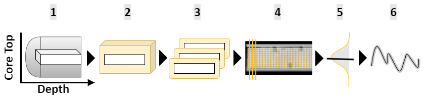
Figure 1 Schematic representation of the triplicate workflow. (1) Subsampling from sediment cores via 30 cm LL-channels (Suigetsu 2006 Project Members and Nakagawa, 2014), used for X-ray photography; (2) freeze-drying and embedding of 5-cm subsections (“pieces”), (3) cryomicrotome cutting onto ITO slides of 3 subsequent 100-µm “slices” per piece; (4) MSI scans; (5) data processing, horizon-wise aggregation & conversion to time series; (6) time series analyses. Orientation of sediment samples and time series is left to right: core top (“recent”) to depth (“past”).

For each 5-cm depth interval of KC1 00–30 cm relative depth, the workflow was repeated on three subsequent slices, yielding triplicate measurements with the minimum achievable distance to the previous measurement area (100 µm cutting thickness).

MSI measurements were inspected and lockmass-calibrated using Bruker Compass DataAnalysis 5.0 SR1. Our main targets were the Na⁺ adducts of di- and tri-unsaturated alkenones (C37:2, C37:3). Each of the shots (orange dots in Fig. 1, step 4) resulted in a mass spectrum from which the intensities of the compounds, as well peak quality (“SNR_FT”) were extracted and used for further analyses, either per spectrum (spotwise-calculated $U_{\mathrm{37}}^K{}^{\prime }$, “swUk”) using the formula

$$\begin{array}{}\text{(1)}& U_{\mathrm{37}}^K{}^{\prime }={\displaystyle \frac{\mathrm{C}\mathrm{37}:\mathrm{2}}{(\mathrm{C}\mathrm{37}:\mathrm{2}+\mathrm{C}\mathrm{37}:\mathrm{3})}}\end{array}$$

(Prahl and Wakeham, 1987) or aggregated per horizon (see Fig. 1, step 4–6 and Sect. 2.5 “Time-Series Analyses”). Peak intensities were only used when passing a SNR_FT quality threshold. Besides alkenones, we utilized pyropheophorbide α as a first-order estimation for primary production and calibrant during FT-ICR-MS lockmass calibration because of its ubiquity in SBB sediments (Liu et al., 2022) and stability over the timescales of this study (Szymczak-Żyła et al., 2011).

During the development of the MSI workflow by Wörmer et al. (2014) and in subsequent studies, the resulting $U_{\mathrm{37}}^K{}^{\prime }$ values were verified using GC-FID measurements (Alfken et al., 2020; Napier et al., 2022; Obreht et al., 2022a, b). Differences in $U_{\mathrm{37}}^K{}^{\prime }$ values obtained by different mass spectrometry techniques have been reported and attributed to varying ionization efficiencies of alkenones, the co-elution of other compounds, and additional factors (Chaler et al., 2000, 2003; Liao et al., 2023; Rama-Corredor et al., 2018). Notably, data derived from MSI in warm SST regions have shown a cold bias compared to GC-FID data, leading to the introduction of site-specific correction factors. However, in the temperate SST regime of SBB, MSI and GC-FID data did not exhibit significant differences and correlated well with CalCOFI buoy SST data at the site (Alfken et al., 2020; California State Department of Fish and Game; NOAA Fisheries; Scripps Institution of Oceanography, 2001).

The calculated $U_{\mathrm{37}}^K{}^{\prime }$ values were then translated to temperature using the calibration of Prahl and Wakeham (1987). Other calibrations are available (Tierney and Tingley, 2018); however, the experimental calibration of Prahl and Wakeham was confirmed by Müller et al. (1998) for 60° S–60° N and the applicability of this calibration for California specifically was supported by Herbert et al. (1998). As our results focus on replicability, they are not sensitive to the choice of calibration.

2.2 Study Area

The Santa Barbara Basin is located in the Southern California Bight and part of the California Current System (Bograd et al., 2019). The basin covers ∼ 110 km² and is separated from the Pacific in the west and the Santa Monica Basin in the east by submarine sills, with the depocenter at ∼ 595 m (Soutar and Crill, 1977). The bathymetric layout, together with seasonal upwelling, high productivity in summer, and high sedimentation rates from winter runoff, can favor the preservation of laminated or varved sediments (Reimers et al., 1990; Thunell et al., 1995). The sediment sequence is interrupted by flood layers (“gray layers”) and mass movements from the upper shelf close to the shore (“massive olive layers”), and bioturbated intervals (Du et al., 2018; Hendy et al., 2013). Oxic time intervals allow colonization by macrofauna, for example, during the Macoma event 1835–1840 (Schimmelmann et al., 1992). During the Holocene and Late Pleistocene, varved, laminated, or bioturbated sections alternated in response to phases of varying oxygenation (Anderson et al., 1990). However, Bernhard et al. (2003) reported microscale bioturbation even under oxygen-limited or anoxic-sulfidic conditions.

2.3 Age Control

We conducted our analyses on depth scale, as the focus was on replicability, which is independent of an exact age scale, and depth- or distance-based interpretations enhance the comparability of our results across different depths and sediment structures within the SBB. For general orientation, we anchored our sediment section KC1 to existing chronologies by identifying flood and event layers in the X-ray imagery (see Supplement Sect. S2). The topmost 0–5 cm relative depth piece contains a flood layer that aligns with the 1761 AD flood layer in SBB (Hendy et al., 2013). The presence of a massive olive-colored layer and partially mixed sections prevented the development of a detailed age model beyond linear interpolation between the 1761 and 1532 AD gray flood layers following approaches such as Zhao et al. (2000) and O'Mara et al. (2019). As a first-order age model to help interpret results of the spectral analyses, we use 1.4 mm yr⁻¹ based on average sedimentation rates and typical varve thickness for compacted sediments throughout SBB during the Holocene (Behl, 1995; Du et al., 2018; Ingram and Kennett, 1995; Schimmelmann et al., 1990; Schimmelmann and Lange, 1996).

2.4 Spatial Analyses

We estimated the spatial correlation structure of the measured compounds and spotwise-calculated $U_{\mathrm{37}}^K{}^{\prime }$ (“swUk”) temperatures using variogram analysis (Cressie, 1993; Maroufpoor et al., 2020; Wikle et al., 2019). For each starting point, “shot” in our case, the semivariance γ between the starting point and all other points in specific distance bins was calculated. We compared differences in horizontal (within horizon, approximately parallel to lamina, see orange lines in Fig. 1, step 4) and vertical (downcore) semivariances as a metric for spatial (dis)similarity. Separation by direction enables the characterization of zonal and geometric anisotropy, which is the directional dependence of the differences or their increase over distance, which can be used to assess the influence of lamina preservation and the homogeneity of deposited horizons. Peak intensities of alkenones and pyropheophorbide α were log10 transformed, scaled, and centered to account for the strong non-normality of the data, whereas spotwise $U_{\mathrm{37}}^K{}^{\prime }$ (swUk) values were used without transformation. For the estimation of the sample variogram, we used the R::gstat implementation (Gräler et al., 2016; Pebesma, 2004; Posit team, 2025; R Core Team, 2024) choosing 100 µm bin widths, together with horizontal and vertical tolerances of 10° to ensure sufficient data coverage and account for deviations in sample or laminae orientation.

2.5 Time-series Analyses

MSI data was mapped to the X-ray density maps using three tie points and an affine transformation to correct for potential sample deformation during embedding and cutting (Alfken et al., 2020) using the Python software msiAlign (Liu et al., 2025). The known flood layer in the upper part of the KC1 segment was identified using X-ray density scans and MSI data, and the respective subsection was excluded from the 0–5 cm interval replicates prior to statistical analyses. Horizons with very low numbers of MSI detections across all compounds (fewer than 10 simultaneous detections of C37:2 and C37:3) were removed. To avoid introducing gaps and ensure sufficient detections per horizon, the minimum horizon width was set to 200 µm. The time series were then formed by summing the intensities of each of the valid alkenone detections (simultaneous detection of both alkenones per shot, where each passes the SNR_FT threshold) within each horizon and calculating the $U_{\mathrm{37}}^K{}^{\prime }$. Short segments of missing horizons due to insufficient detections were linearly interpolated. On average, ∼ 4 % of horizons were missing: ∼ 1.4 % at the ends of series and ∼ 2.7 % within.

Following Laepple and Huybers (2014), power spectral density (PSD) estimates were calculated on linearly detrended, centered data using the multitaper method with three tapers and a time-bandwidth parameter of ω=2 (Thomson, 1982). The PSD estimates were smoothed using a Gaussian kernel with a constant width of 0.2 on the logarithmic timescale (base 10) (Kirchner, 2005), and the three lowest and highest frequencies were omitted.

We followed the framework developed by Münch and Laepple (2018), based on a partitioning of variance approach (Fisher et al., 1985), to separate the climatic signal and noise contributions in the spectral domain. We defined the climate signal as the common signal shared between the time series of a depth interval. The residual, individual variations, formed the noise component and allowed the quantification of the shared signal as signal-to-noise ratios.

Given a regional cluster of n proxy records with a similar climate between sites, the mean power spectrum, M, averaged across all individual records' spectra, will yield a precise estimate of the proxy spectrum. In contrast, the power spectrum S of the stacked record from averaging all datasets in the time domain will also contain the full common signal, but with the noise proportions reduced by a factor of n. By combining both quantities one can derive expressions for the climate and noise spectra (McPartland et al., 2024; Münch and Laepple, 2018)

$$\begin{array}{}\text{(2)}& {\displaystyle }& {\displaystyle }C={\displaystyle \frac{n}{n-\mathrm{1}}}\left(S-M/n\right)\text{(3)}& {\displaystyle }& {\displaystyle }N={\displaystyle \frac{n}{n-\mathrm{1}}}\left(M-S-{\displaystyle \frac{n-\mathrm{1}}{n}}\right)\end{array}$$

with the ratio of C:N yielding the frequency-resolved signal-to-noise ratio (SNR). We further compute the integrated SNR which yields the SNR of the time-series that one obtains if one measures at a specific sampling resolution

$$\begin{array}{}\text{(4)}& {\mathrm{iSNR}}_{f\left(Nyq\right)}={\displaystyle \frac{{\int }_{\mathrm{0}}^{fNyq}{C}_f}{{\int }_{\mathrm{0}}^{fNyq}{N}_f}}\end{array}$$

The relation of SNR to correlation can be found in the Supplement (Sect. S3), however as direct climatic interpretation is not the focus of this study, we report shared signal content between replicates expressed as SNR throughout the manuscript.

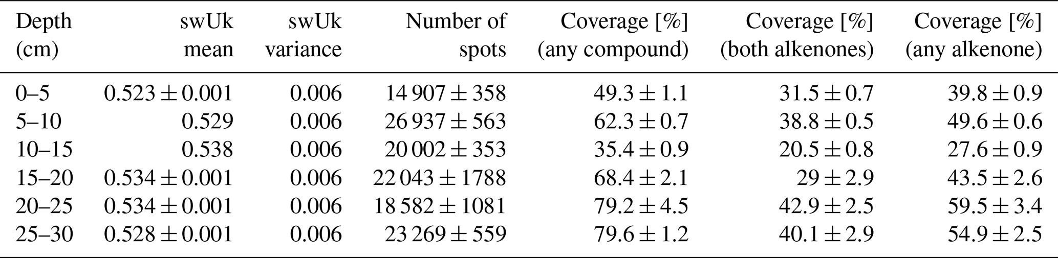
Table 1 Map statistics averaged across replicates per depth interval. For “swUk mean” spotwise-calculated $U_{\mathrm{37}}^K{}^{\prime }$ values have been averaged for the replicate maps and subsequently per 5-cm depth interval. Accordingly, swUk variance is the average variance of swUk values (“field variance”) of the replicate maps per depth interval. $U_{\mathrm{37}}^K{}^{\prime }$ units have been rounded to three digits, S.E. below 0.001 (∼ 0.03°C) are not shown.

3 Results

3.1 Characterization of MSI maps

The measurement areas ranged from 14 907 to 26 937 laser shots for each 5-cm slice (20 957 ± 4134 = 1σ), and thus ∼ 40 shots per 100-µm horizon. On average, at 62 % of the shots, at least one of the three compounds was detected. Pyropheophorbide α was detected in 61 % of the spectra, while at least one alkenone was detected in 46. Both alkenones were detected simultaneously in 34 % of the spectra, which could then form swUk estimates (spotwise-calculated $U_{\mathrm{37}}^K{}^{\prime })$. When aggregating 200-µm horizons to time series, these detection rates amounted to ∼ 37 shots on average that yielded at least one alkenone compound and an average of ∼ 31 simultaneous detections per horizon (see Tables 1 and S5 in the Supplement).

We first investigated the replicability and signal content of individual MSI maps in terms of the similarity of their overall swUk (spotwise-calculated $U_{\mathrm{37}}^K{}^{\prime })$ values and distributions. The swUk maps showed strong spatial heterogeneity (Fig. 2B). Despite this, the average values were highly consistent between MSI replicates: the standard error of the mean swUk per triplicate was just 0.001, corresponding to ∼ 0.03 °C (Prahl and Wakeham, 1987). Similarly, the level of spatial variability was consistent across the replicates. The average swUk variance within maps (“field variance”) was 0.00595±0.00004, corresponding to 2.34 ± 0.19 °C. The swUk distributions were similar across depth intervals and were unaffected by sediment structure (Fig. 2C).

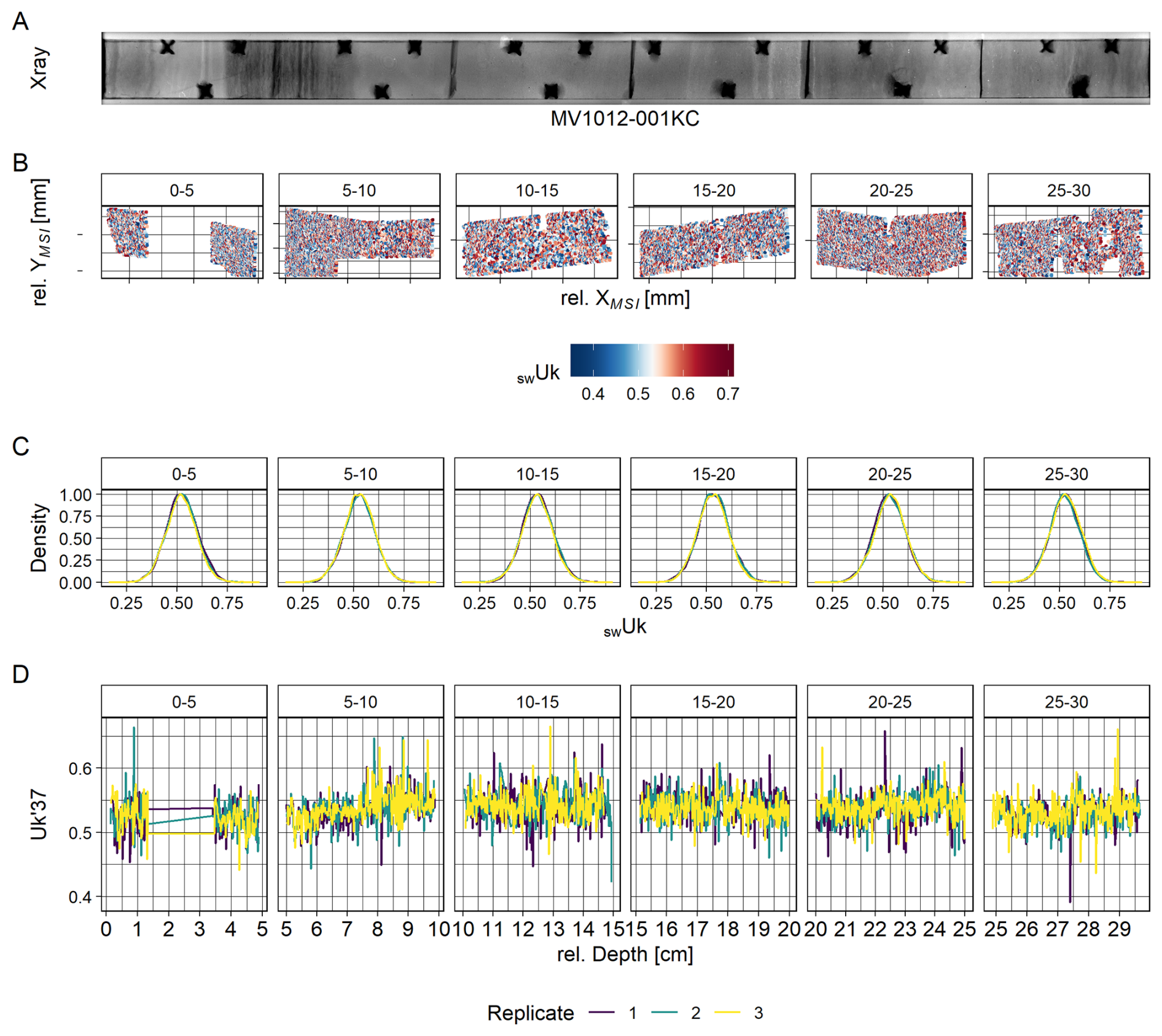
Figure 2 Maps and time-series of sediment section KC1. (A) X-ray density map with black crosses or rectangles where material was removed as markers for orientation of the samples, (B) exemplary swUk (spotwise $U_{\mathrm{37}}^K{}^{\prime })$ maps of one replicate per depth interval. Maps are shown on the MSI coordinate grid before affine transformation onto X-ray coordinates. swUk values below the 1 % and above the 99 % quantiles were removed for improved color scaling during plotting. (C) Scaled density plots of the spatial swUk maps per replicate. (D) Resulting $U_{\mathrm{37}}^K{}^{\prime }$ time-series per replicate and depth interval. Note that the area corresponding to the 1761 AD floodlayer in depth interval 0–5 cm was removed prior to analyses. For (A), (B) and (D) the directionality is from left (“modern”) to right (“past”). A minor exposure artefact was removed from the X-ray photography of KC1 at ∼ 24 cm. An unaltered version can be found in the Supplement (Sect. S4).

Values from the same horizon can be aggregated into a single data point, and thereby, a time series can be constructed. The average variance of swUk (spotwise $U_{\mathrm{37}}^K{}^{\prime })$ in these 200 µm horizons was similar to the observed total field variances: 0.006±0.00005 (2.35 ± 0.21 °C, Supplement Sect. S5). A visual comparison between replicate time-series showed good agreement in terms of mean values and slow variation (Fig. 2D), yet weak correlation of the fastest resolution of 200-µm steps, with an average Pearson's r of 0.12 and average RMSE of 0.03 (∼ 0.89 °C). Such weak correlations most likely result from a lack of fine-scale depth alignment.

3.2 Microscale Analyses of Spatial Heterogeneity

After confirming consistency between replicates on a coarse whole-slice level, we examined the spatial proxy heterogeneity using maps of spotwise-calculated $U_{\mathrm{37}}^K{}^{\prime }$ values (swUk). These spatial patterns showed high variability both across depth and laterally, with average swUk variances across depths and horizons both approximating 0.00596 (vertical, downcore: 0.00597; horizontal: 0.00596).

To explore the structure of this heterogeneity in more detail, we focused on two representative depths, one laminated and one mixed, along with their respective replicates (Fig. 3). Notably, the clear laminations observed in the X-ray scans (e.g., at 5–7 cm; Fig. 2A, top row) are not reflected in the swUk patterns. Instead, both laminated and mixed intervals show swUk values forming small clusters of neighboring pixels with similar temperatures.

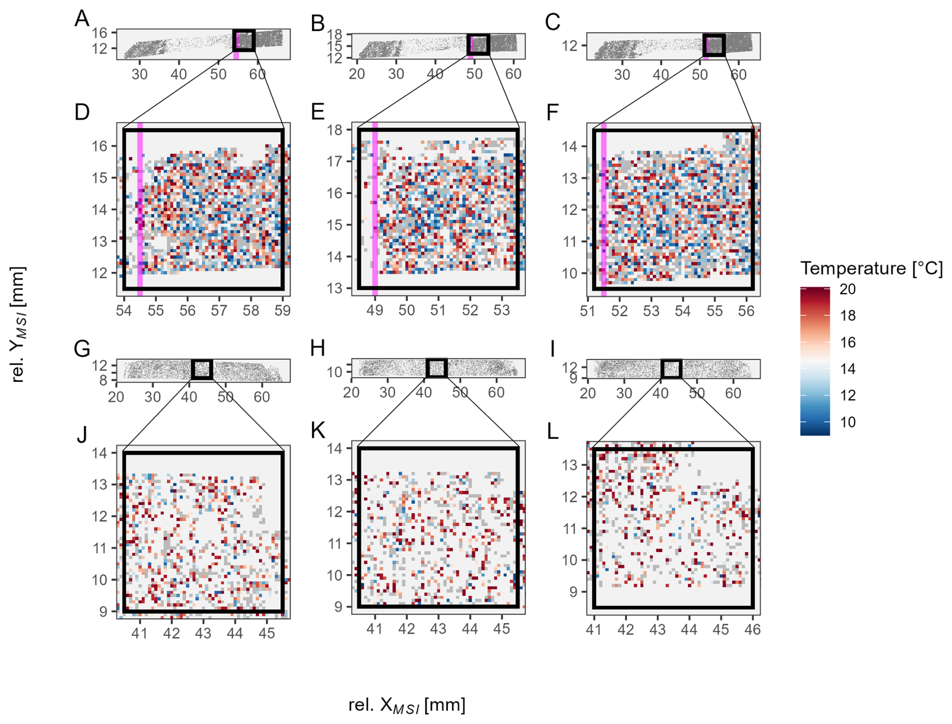
Figure 3 Overview maps of the measurement areas for three replicates from 0–5 cm (A–C) and 10–15 cm (G–I) depth: gray areas indicate spots in which alkenones were successfully detected. Downcore direction is from left to right, y axes correspond to layers parallel to the sediment surface. Pink line: onset of the 1761 AD flood layer; black rectangles indicate 5×5 mm inlets, as shown in (D–F) and (J–L). These zoom-ins show values for swUk (spotwise $U_{\mathrm{37}}^K{}^{\prime })$ converted to SST (Prahl and Wakeham 1987). (D)–(F) represent a laminated interval below the flood layer, while (J)–(L) correspond to a thoroughly mixed interval of KC1 (“olive turbidite”, event 1D in Hendy et al., 2013). Maps are shown as measured, before affine transformation onto X-ray coordinates.

To describe local (dis) similarities in biomarker patterns more precisely, we obtained averaged variogram estimates of the compounds and swUk. This approach revealed that only a small portion of total variability is spatially structured (Table 2) in KC1. The total map-level variance, the “sill” in the variograms, was 0.00595 (∼ 2.34 °C), of which only 0.0002 (∼ 0.43 °C) showed small-scale spatial structure, that is, clustering or increased similarity among neighboring values. Most of the variability (∼ 93 %–99 %, avg. 96 %) is unstructured or unresolved, termed the nugget effect (C₀). A high contribution of C₀ can indicate variation, which is either spatially unresolved, intrinsic variability of the proxy, or measurement noise. In contrast, pyropheophorbide α showed a slower decay of similarity with distance and a lower C₀ “nugget” component (80 %–96 %, avg. ∼ 86 %), indicating stronger spatial structure (Fig. 4A, C green lines).

Table 2 Estimated swUk variogram parameters averaged per 5 cm depth interval (pieces).

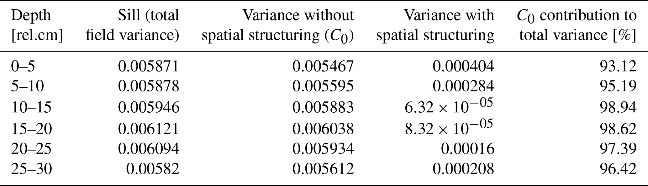
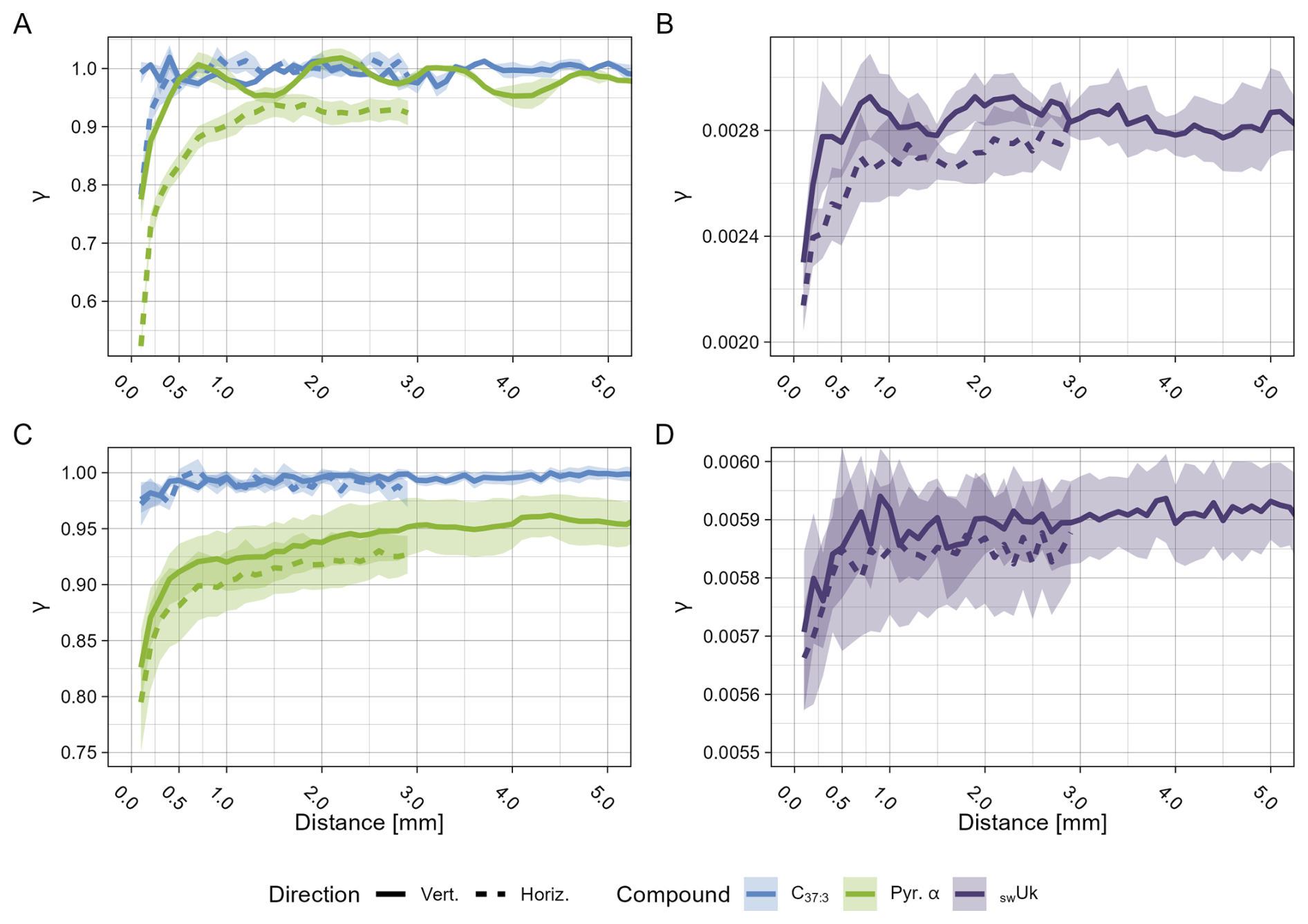
Figure 4 Variogram estimates of pyropheophorbide α and C37:3 intensities and swUk (spotwise $U_{\mathrm{37}}^K{}^{\prime })$ temperatures, showing the semivariance or dissimilarity of pairwise spot comparisons (γ) as a function of distance. Solid lines indicate sample variogram estimates along the vertical, downcore direction of the original sediment position; dashed lines indicate within-layer estimates, parallel to the sediment surface. (A) and (B) are obtained for the exemplary varved section of SBX, averaged over 3 replicates. (C) and (D) for sediment segment KC1, averaged over all replicates and depth intervals ($\mathrm{3}\times \mathrm{6}\times \mathrm{5}$ cm). Note that each panel has individual y-axes, as pyropheophorbide α and C37:3 values in (A), (C) were scaled prior to calculation and are not in their native units, whereas in (B), (D) γ values correspond to $U_{\mathrm{37}}^K{}^{\prime }$ units.

We then separated vertical from horizontal similarity to distinguish between variability across successive depositional layers (in situ vertical, downcore) and within the same horizon (horizontal). It is important to note that the spatial plots in Figs. 2B and 3 are rotated by 90° to align with time-series convention; therefore, variograms estimated over the vertical downcore direction in the original sediment position have to be visualized left to right on these plots. As a proof of concept, we also applied this approach to a varved interval from a box core as the best-case reference without sediment mixing (Alfken et al., 2020, 2021). In both sample sets, this separation (solid lines: original sediment position vertical, downcore; dashed: horizontal, Fig. 4) reveals geometric anisotropy: similarity decreases more slowly in the horizontal than in the vertical direction. This can be interpreted as the within-horizon variability, parallel to the sediment surface, (dashed) which is lower and increases more gradually with distance than between layers (solid). This pattern is most clearly visible in the intensity data of pyrophophorbide α, but is also detectable in the C_37:3 alkenone and spotwise $U_{\mathrm{37}}^K{}^{\prime }$ data. As expected, the differences were clearer in the varved section of SBX than in the combined core KC1. Notably, in the varved section, pyropheophorbide α and, to a lesser extent, $U_{\mathrm{37}}^K{}^{\prime }$ show a sinusoidal pattern in γ with a distance between peaks and troughs that matches reported average annual sedimentation rates of ∼ 1.4 mm (Behl, 1995; Du et al., 2018; Ingram and Kennett, 1995; Schimmelmann et al., 1990). Variograms of individual sediment slices can be found in the Supplement (Sect. S6).

3.3 Frequency-dependent Signal and Noise Components of Replicated Time-Series

Replication within 5-cm depth intervals allowed us to quantify the reproducibility between individual MSI slices and estimate the SNR of the resulting time-series. The frequency-dependent separation of the shared signal and independent noise shows that the replicates contain increasing signal content with timescale and flat noise spectra. Signal spectra showed an average slope of $\sim -\mathrm{1.7}$ estimated between $f=\mathrm{1}/\mathrm{10}$ mm⁻¹ and $f=\mathrm{1}/\mathrm{2}$ mm⁻¹, the interval of the spectral estimates not affected by bias and gaps. The noise components showed no frequency dependency ($\sim -\mathrm{0.13}$ between $f=\mathrm{1}/\mathrm{10}$ mm⁻¹ and $f=\mathrm{1}/\mathrm{2}$ mm⁻¹, see Fig. 5A).

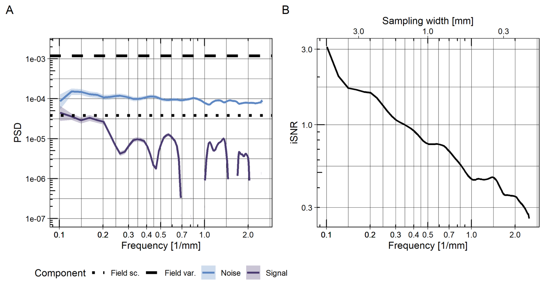
Figure 5 Frequency-dependent signal and noise components in comparison to field variance (A) and the resulting integrated SNR (iSNR) estimate (B). The dashed line shows the average variance of the swUk field in black; the dotted line is the field variance downscaled by the average number of swUk shots per horizon, imitating the noise reduction during time series processing.

As a reference, we added noise spectra derived from total field variance (black dotted line, Fig. 5A), downscaled by a factor of ∼ 37, the average number of swUk measurements per horizon at 200 µm resolution (see also Table 2), to illustrate how independent (measurement) noise scales with averaging. The actual noise level was ∼ 13 higher than this baseline, indicating a noise reduction weaker than $\mathrm{1}/n$ when aggregating to horizonwise $U_{\mathrm{37}}^K{}^{\prime }$ data.

Integrating the spectra from high to low frequencies yields the integrated SNR (iSNR), which is an estimate of the expected SNR at a given sampling resolution. iSNR values reach from ∼ 0.24–∼ 3.1, considering sampling from submillimeter to centimeter steps (Fig. 5B).

We then assessed the influence of sediment structure on time-domain signal-to-noise variance ratios (Fisher et al., 1985) (that is SNR between the variance of the noise and signal components) of the different depth intervals in comparison to the “best case” varved 5 cm section published earlier (Alfken et al., 2020, 2021). We also repeated the analysis using different aggregation steps (Fig. 6) to assess the impact of data processing choices. The tested sampling widths ranged from 200 to 1400 µm, which, under ideal preservation and an average sedimentation rate of 1.4 mm yr⁻¹, would correspond to monthly to annual resolutions. For core segment KC1, these SNRs ranged from ∼ 0 in the most strongly mixed interval to ∼ 2 in an interval with partially preserved varves (Fig. 6). In comparison, the varved section of SBX reached SNRs of ∼ 2.8 on average.

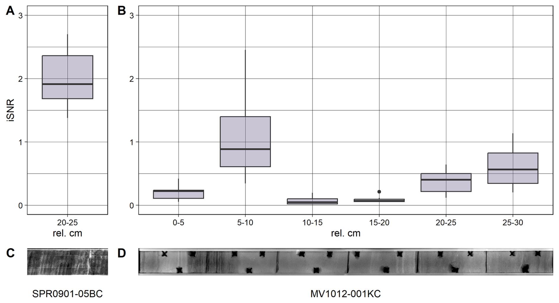
Figure 6 Comparison of sediment structure and SNR based on time domain signal-to-noise variance ratios (Fisher et al., 1985), resulting from aggregating horizons from 0.2 to 1.4 mm, the theoretical maximum aggregation for annual resolution. (A) and (C) show a 5 cm exemplary interval from the varved upper part of SBB (ca. 1913–1935). (C) and (D) show the KC1 segment which represents the different conditions found at SBB throughout the late Holocene, ranging from laminated sediments, varying degrees of mixing to turbidites. Note that the 1761 AD flood layer in KC1 0–5 cm was removed from the time-series prior to SNR estimation. (C) and (D) are X-ray density maps of the respective samples, brighter colors indicate denser material. Black holes are markers for orientation during sampling and for correcting distortion. A minor exposure artefact was removed from the X-ray photography of KC1 at ∼ 24 cm. An unaltered version can be found in the Supplement (Sect. S4).

4 Discussion

This study investigated the spatial heterogeneity of biomarkers at submillimeter resolutions and its effect on the time-scale-dependent signal-to-noise ratios of MSI-based high-resolution SST reconstructions. In the following sections, we discuss the observed spatial heterogeneity of biomarkers and the influence of sediment mixing intensity on the interpretability of high-resolution SST reconstructions.

4.1 Spatial Heterogeneity of Biomarkers

Variogram analyses showed greater similarity across sedimentary horizons than downcore (Fig. 4, dashed and solid lines), consistent with the expectation of layered archives, where variation over depth includes additional variability from changing climate signals over time (Fisher et al., 1985; Münch and Laepple, 2018).

Biomarker maps revealed sub-millimeter-scale clustering and marked differences in spatial heterogeneity between compounds (Figs. 4, 5). For swUk, the variance that exhibited spatial structuring was minimal (∼ 4 %). The small-scale clustering (ranges ∼ 0.5 mm) observed in the biomarker maps implies that, for optimal sampling, MSI measurement windows should be in the range of a few millimeters to be wide enough to (1) have enough successful shots to overcome sparse detections and (2) avoid bias or correlated noise that could arise from only targeting single proxy clusters. Therefore, the typical measurement window widths of ∼ 4–8 mm used in this and earlier studies (Alfken et al., 2020, 2021; Liu et al., 2022; Napier et al., 2022; Obreht et al., 2022b; Wörmer et al., 2014, 2022b) should effectively reduce the noise in downcore records.

Under favorable sediment preservation conditions, varved sections manifest as oscillations in the variogram (Fig. 4A, green solid lines and B, purple solid lines). These can be interpreted as the results of measuring downcore, leaving areas of values that were deposited during a similar time interval and seasonal conditions, which increases average dissimilarity (γ, semivariance of pairwise comparisons as a function of distance), before dissimilarity decreases again when the values from these distances begin to again resemble the starting conditions. For example, when moving into sediments of the same preceding seasons. Therefore, peaks and throughs represent the differences between contrasting or identical seasons, respectively, and the typical distances between the same seasons match reported average sedimentation rates at SBB (Behl, 1995; Du et al., 2018; Ingram and Kennett, 1995; Schimmelmann and Lange, 1996).

The high proportion of unstructured variance in our biomarker and proxy maps suggests significant noise at the individual spot level. Aggregating data across horizons enhances the signal content because noise is largely uncorrelated between spots at the microscale. However, the data from this study does not allow us to determine whether this noise stems from measurement errors or the deposition of heterogeneous biomarker signals. Strong shot-to-shot variation is a common issue in MSI (Tobias and Hummon, 2020). On the other hand, classic bulk sediment $U_{\mathrm{37}}^K{}^{\prime }$ estimates reflect averaged or smoothed signals, and it is difficult to estimate potentially contained heterogeneity. Observed variability is influenced by the temporal and spatial scales that are aggregated within each sample. For instance, water column and sediment trap data display a broader range of $U_{\mathrm{37}}^K{}^{\prime }$ values around measured ocean temperatures than core tops (Conte and Eglinton, 1993; Freeman and Wakeham, 1992; Herbert et al., 1998). Our observed proxy spot-level variance is smaller than that of the monthly SST estimates for SBB, but larger than the interannual variation (Sect. S7), suggesting that the observed heterogeneity may indeed originate from SST and capture variability typically lost in bulk sediment samples. MSI-based $U_{\mathrm{37}}^K{}^{\prime }$ maps could help bridge processes along the proxy formation chain by resolving within-bulk-sample variability, and may provide access to high-frequency climate variability, including intraannual variations. This parallels developments in foraminiferal isotope proxies, where analyses of individual foraminifera complement bulk measurements (Glaubke et al., 2021) and have been argued to resolve seasonal to interannual variability.

4.2 Timescale dependent signal to noise estimations

Averaging across a diverse range of sediment preservation conditions in core segment KC1, we detected iSNRs around ∼ 1 at interannual resolution, increasing to 3 at subdecadal (ENSO) resolution. The extracted noise component shows no dependence on time scale, whereas the variance of the signal components increases with time scale. This suggests that temporal aggregation effectively reduces noise in individual time series and enhances the relative potential climate signal content. Additionally, stacking multiple replicates would further decrease the noise contribution by a factor of $\mathrm{1}/n$, boosting the relative signal content.

An iSNR ≫ 1 indicates that individual MSI series are representative of their core samples and demonstrate potential for high-resolution climate reconstructions at subdecadal resolution in the case of the SBB sedimentary archive containing laminated and mixed intervals. This aligns with findings of O'Mara et al. (2019), who estimated the effective temporal resolution of neighboring laminated SST records from San Lazaro Basin to approximately decadal without replication or stacking.

One limitation of our method is its sensitivity to depth misalignment between replicates, which could lead to a bias in SNR estimates at the fastest temporal and corresponding spatial scales (≪1 mm). To minimize these effects, we used sediment marker holes and mapped the MSI data onto X-ray imagery. More advanced image correction and alignment may further reduce these biases in the future. However, low SNRs at ≪1 mm also match expectations based on reports by Bernhard et al. (2003), who documented living microorganisms such as ciliates, foraminifera, and bacterial colonies growing under severe oxygen limitation, even within otherwise undisturbed laminae, pointing to an alternative cause for the low SNRs at the fastest resolutions.

The current SNR estimates are based on closely spaced samples (cryotome cuts within <1 mm horizontal distance) to provide as identical conditions as possible under natural conditions to estimate the baseline noise level for individual MSI-derived $U_{\mathrm{37}}^{k^{\prime }}$ time-series. This leads to the tradeoff that spatially correlated noise between adjacent cuts may also be interpreted as a shared signal, effectively barring the direct interpretation of the derived SNRs in terms of a pure climatic signal. However, the correlation of ∼ 0.6 between the MSI-derived $U_{\mathrm{37}}^{k^{\prime }}$ time series and in situ 0–30 m water column temperatures reported by Alfken et al. (2020) is close to the upper achievable limit of ∼ 0.77 as suggested by our SNR estimates for the exemplary varved pieces (Figs. 6A and S3). Together with the short-range spatial similarity found in the variogram analyses (Fig. 4) we expect correlated noise between replicates to play a minor role. Future studies using samples at larger lateral spatial scales (for example nearby sediment cores) combined with longer core segments will help to better characterize and separate the spatial structure of signal and noise components.

4.3 The influence of lamina preservation

Variogram analyses demonstrated that the degree to which a spatial structure is preserved in the sedimentary archive strongly influences the spatial variation patterns of biomarkers. Under strong mixing conditions, such as olive turbidite 1D ∼ 1738 AD (Hendy et al., 2013), horizontal variation and variation over depth are similar. However, as lamina preservation increases, the anisotropy of the variograms becomes more pronounced, with longer ranges of similarity within horizons and generally greater variation over depth, suggesting potential additional climate variation (see also Sect. S6). Additionally, the variogram of a varved example section from the early 20th century captures the rhythmic seasonal variation of the biomarkers over depth (Fig. 4A green solid line), whereas this seasonal pattern is destroyed in the lower sediment sections.

Across a broad, yet plausible range of processing choices, the influence of sediment structure was the dominant factor affecting the high-frequency replicability (SNR) between individual MSI time-series. The achieved SNRs at sub-millimeter to interannual (∼ 1.4 mm) sampling closely follow the degree of preservation of lamina, as visible in the X-ray (Fig. 6C, D). Earlier studies have shown that the mixing and bioturbation intensities assessed in this study are representative of Holocene and Late Pleistocene SBB sediments (Anderson et al., 1990; Behl, 1995) and are closely linked to warm phases, which might limit the potential of high-resolution MSI variability estimates to snapshots during favorable oceanic regimes.

5 Conclusions

Recent methodological advances allow the measurement of biomarkers and sediment proxies with increasingly fine spatial resolution, significantly enhancing the potential for reconstructing high-resolution climate variability from the past, well beyond the scope of instrumental records. Our analysis of replicated MSI-based biomarker maps from a single Santa Barbara Basin core reveals how spatial variability reflects both the preservation state of the sediment and the fidelity of SST proxy signals. We show that biomarkers in marine sediments display significant heterogeneity, even within uniformly deposited horizons and well-preserved laminae. This variability might serve as the missing link needed to reconcile smooth bulk sediment SST estimates with the more variable results from water column and sediment trap studies. The degree of lamina preservation is the primary factor controlling proxy replicability. In laminated intervals, signal-to-noise ratios increase with temporal scale, reaching values suitable for subdecadal interpretations, even when using single MSI measurements. In contrast, mixed sediments show reduced signal content, particularly at higher frequencies, limiting the resolution of the interpretable variability.

To fully exploit the potential of MSI-based time series, further refinement of data processing methods is needed to minimize noise introduced during the conversion of spatial measurements to SST estimates. Regional replication is also essential for isolating shared climate signals and suppressing locally correlated noise. With optimized workflows and stacking approaches, MSI-derived SST records from the Santa Barbara Basin show strong potential to continuously resolve the range from interannual to centennial variability throughout the Holocene and Late Pleistocene, offering a powerful complement to existing paleoclimate archives.