Possible provenance of IRD by tracing late Eocene Antarctic iceberg melting using a high-resolution ocean model

The Eocene–Oligocene transition (EOT) is characterised by the inception of the large-scale Antarctic ice sheet. However, evidence of earlier glaciation during the Eocene has been found, including the presence of ice-rafted debris (IRD) at Ocean Drilling Program (ODP) Leg 113 Site 696 on the South Orkney Microcontinent (SOM) (Carter et al., 2017). This suggests marine-terminating glaciers should have been present in the southern Weddell Sea region during the late Eocene, generating sufficiently large icebergs to the South Orkney Microcontinent to survive the high Eocene ocean temperatures. Here, we use Lagrangian iceberg tracing in a high-resolution eddy-resolving ocean model of the late Eocene (Nooteboom et al., 2022) to show that icebergs released from offshore the present-day Filchner Ice Shelf region and Dronning Maud Land could reach the South Orkney Microcontinent during the late Eocene. The high melt rates under the Eocene warm climate require a minimum initial iceberg mass on the order of 100 Mt and an iceberg thickness of several tens of metres to be able to reach the South Orkney Microcontinent. Although this places the iceberg mass at the larger end of the present-day range of common iceberg masses around Antarctica, the minimum estimates are not unfeasible; hence, the present study confirms previous findings suggesting glaciation and iceberg calving were possible in the late Eocene.

1 Introduction

A period of long-term global cooling through the middle and late Eocene, interrupted by the relatively short but warm Middle Eocene Climatic Optimum (MECO; 40 Ma), eventually set the stage for the formation of a continental-scale Antarctic ice sheet around the Eocene–Oligocene transition (EOT) at roughly 34 Ma (Hutchinson et al., 2021) as CO₂ concentrations declined below threshold levels required for ice formation (DeConto and Pollard, 2016; Pagani et al., 2011). The Antarctic continent is generally considered to be largely ice-free until the end of the Eocene (Singh et al., 2022; Zachos et al., 2001), when an abrupt increase of 1.2 ‰ to 1.5 ‰ is observed in the global marine benthic δ¹⁸O record (Miller et al., 1987; Tigchelaar et al., 2011), which, after removing the temperature component, corresponds to an increase in global ice volume equivalent to 60 % to 130 % of the modern East Antarctic Ice Sheet volume (Bohaty et al., 2012).

However, multiple proxy-based studies have shown evidence for the presence of ice on Antarctica before the EOT, such as around 37.5 Ma (Scher et al., 2014), 36 Ma (Peters et al., 2010), and 36.5 Ma (Carter et al., 2017). This latter study is based on the finding of significant amounts of fine-grained ice-rafted debris (IRD) at Ocean Drilling Program (ODP) Leg 113 Site 696, taken on the southeastern margin of the South Orkney Microcontinent (SOM; Fig. 1). As iceberg calving only occurs when glaciers are marine-terminating (Diemand and Dryak, 2019), this suggests that vast amounts of ice were already present at this time (Carter et al., 2017). In turn, this would require sufficient snow supply to Antarctica to maintain the mass balance under the still relatively high Eocene temperatures (Baatsen et al., 2024; Douglas et al., 2014; Thompson et al., 2022; Nooteboom et al., 2022), although these high temperatures themselves could have led to increased precipitation on Antarctica (following the Clausius–Clapeyron relation; Le Treut and Ghil, 1983). In combination with a suitable topography, creating sufficiently low temperatures at higher altitudes for snowfall to survive the summers, this could have allowed glacier formation. Still, such high temperatures would imply that icebergs, if present, would have been relatively short-lived (Carter et al., 2017) or relatively large in size, thereby lengthening their lifetime and allowing them to travel larger distances (Wesche and Dierking, 2014). In addition, if glaciers were present in the late Eocene, the local temperature might be somewhat overestimated, as the fully coupled climate models do not include ice–climate interactions.

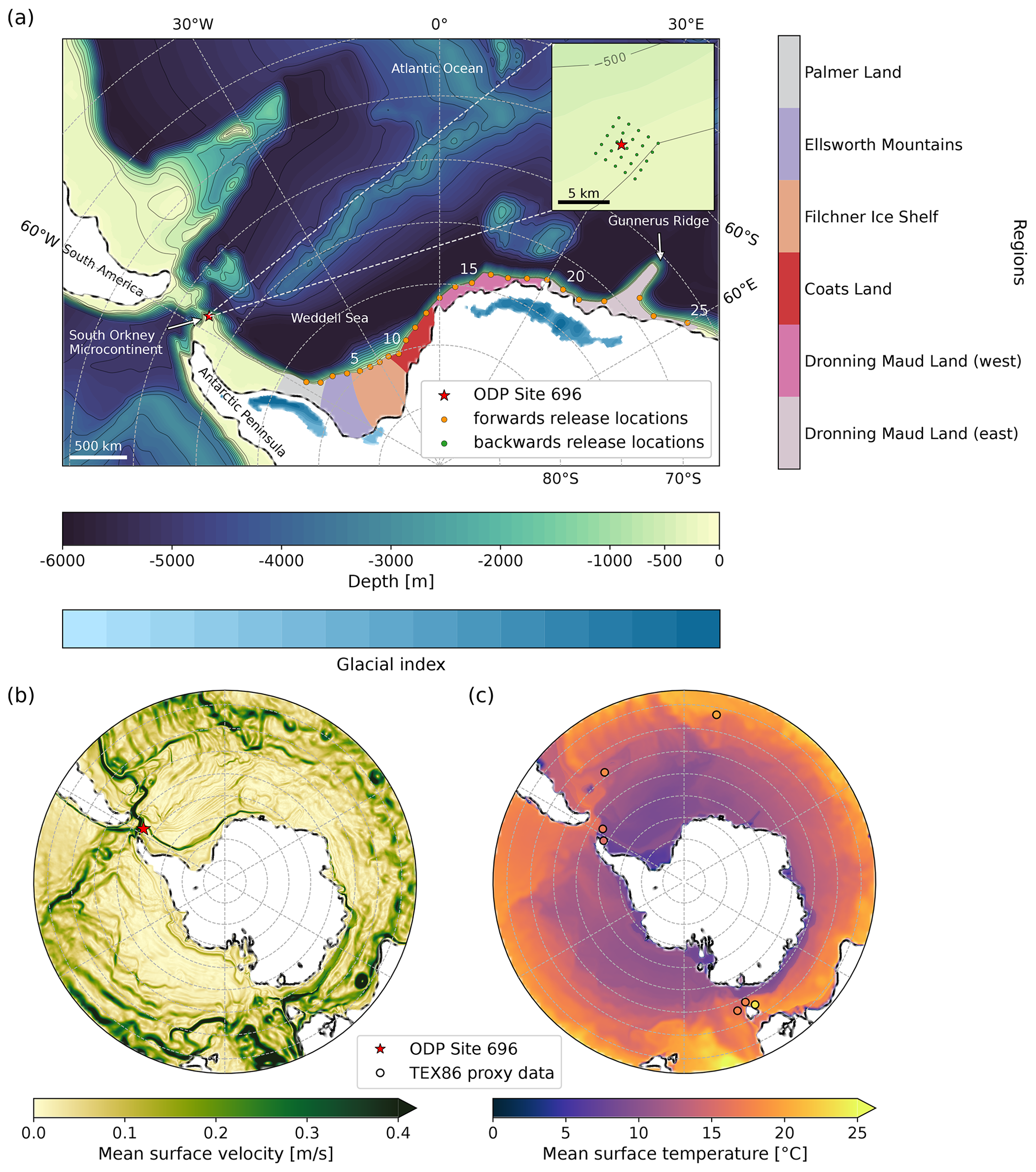
Figure 1 Eocene geography of the Weddell Sea region (Nooteboom et al., 2022) with (a) the approximate location of ODP Site 696 and the 25 forward and 25 backward iceberg release locations defined in this study. Also shown are the potential provenance regions from Palmer Land to Dronning Maud Land based on Carter et al. (2017) and potential regions of ice formation during the late Eocene as given by a glacial index calculated from a simple surface mass balance by Baatsen et al. (2024). Regional time-mean (model years 38–42) ocean properties from the high-resolution late Eocene model fields by Nooteboom et al. (2022) are given for (b) the velocity in the surface layer and (c) the temperature at the surface (∼ 0–200 m). The latter panel includes TEX₈₆ surface (∼ 0–200 m) temperature data from the late Eocene for ODP sites 1172, 1170, 1090, 1168, and 696; DSDP Site 511; and Seymour Island. Note that the marker of ODP Site 696 is roughly one-quarter of the size of the SOM in panel (a) or roughly equal to the size of the SOM in panel (b).

Nevertheless, the formation of a substantial mass of ice before the EOT would complicate the mass balance of δ¹⁸O, as this should have led to an earlier positive shift in oxygen isotopes, which is not obvious in the record (Bohaty et al., 2012) and does not fit sea level estimates (Wilson et al., 2013). Most modelling studies also do not support such large-scale glaciations (Baatsen et al., 2024), although a recent study using a novel ice sheet–climate modelling approach showed that large-scale, though short-lived, glaciations might have been possible when CO₂ levels were sufficiently low and coincided with summer insolation minima (Van Breedam et al., 2022), such as during the Priabonian oxygen isotope maximum (PrOM) at 37 Ma (Scher et al., 2014). In addition, ice–climate interactions are not included in these models, which could thus lead to a much warmer local environment than with ice present.

From the geochronology analysis of the IRD from ODP Site 696 and comparison to the Antarctic continental geology, Carter et al. (2017) indicated the southern Weddell Sea region as the likely source region, whilst a contribution from the nearby Antarctic Peninsula was excluded. Hence, this implies that local ocean currents in the late Eocene should have been relatively similar to today in order to bring the icebergs from the southern Weddell Sea region to ODP Site 696 at the SOM (Fig. 1), next to the icebergs being large enough in size to survive the flow path from Antarctica to ODP Site 696. Currently, the SOM is located in the so-called Iceberg Alley, where most icebergs formed at the Antarctic continent float equatorward (Carter et al., 2017). Indeed, such a local circulation in the Eocene Weddell Sea would be consistent with information from microfossil assemblages (Bijl et al., 2011; Sauermilch et al., 2021) and model simulations (Huber et al., 2004; Sijp et al., 2011).

Therefore, this study aims to reconstruct possible Antarctic iceberg trajectories in the late Eocene and compare these to proxy evidence found at ODP Site 696 by adding iceberg melt parameterisations to Lagrangian tracks of floating particles in an Eocene ocean model. Although reconstructions of late Eocene temperature gradients cannot generally be reconciled with plankton-based circulation patterns in current numerical models (Baatsen et al., 2020), a high-resolution (0.1°) eddy-resolving ocean model of the late Eocene was found to agree better with the circulation patterns and temperature estimates from proxies (Nooteboom et al., 2022), making this model potentially suitable for analysing whether icebergs could have brought IRD to ODP Site 696 at the SOM. If the IRD is indeed derived from Antarctica, as suggested by Carter et al. (2017), the simulations must demonstrate (1) that icebergs derived from the southern Weddell Sea region can indeed reach ODP Site 696 before having melted away, (2) which regions are most likely to have released icebergs, and (3) what the minimum size of the icebergs leaving Antarctica must be in order to survive the flow path from Antarctica to ODP Site 696. Otherwise, the question arises of what causes the disagreement between the IRD and model data, for example, a difference in circulation or temperatures too high for icebergs to survive in.

In the following text, we will first describe the model frame used in this study (Sect. 2), detailing the iceberg model with the underlying assumptions and limitations, describing the forcing (ocean) model and explaining the selection and setup of seed points and the design of the simulations. Then, we will describe the results (Sect. 3), starting from the iceberg trajectories; relate these to the IRD provenance and the iceberg sizes; and finally study the sensitivity of the simulations to several conditions. The Discussion (Sect. 4) largely follows the same structure as Sect. 3 but has an additional section discussing the sensitivity to melt rates. Finally, the conclusion (Sect. 5) summarises the main findings and suggests directions for future research related to the limitations of the current research.

2 Methods

2.1 Iceberg model

In this study, icebergs are traced in a Lagrangian framework using Parcels (Delandmeter and van Sebille, 2019). By adding iceberg melt parameterisations, the size-dependent trajectories of icebergs can be modelled as the size of an iceberg (and, consequently, the depth it reaches) changes with time and hence determine the influence of the horizontal circulation on the iceberg drift. Note that, in this model, the depth-integrated iceberg drift is forced solely by the ocean velocity field so that the influences of wind drag, the direct impact of the Coriolis force on (large) icebergs, wave radiation force, and pressure force are ignored (Sect. S2.1.4 in the Supplement). This approximation works well for large icebergs but can lead to deviations in the trajectories for small (≤ 1 km) icebergs, which experience a stronger influence of wind drift (Wagner et al., 2017b).

2.1.1 Iceberg shape and size

Icebergs exist in a wide range of shapes and sizes that are always irregular to at least some extent. To simplify the simulations, we follow the previous literature (e.g. Rackow et al., 2017; Martin and Adcroft, 2010) and approximate the icebergs as cuboids. We assume a length-to-width ratio of $L:W=\mathrm{1.5}:\mathrm{1}$, consistent with modern observations (Bigg et al., 1997). The thickness or height H of an iceberg consists of a part above water, the freeboard or sail F, and a submerged part, the draft or keel D, following $H=F+D$. Moreover, the draft and thickness are related through density as D=αH, where α is the ratio of the typical iceberg density in the Southern Ocean ρ_i=850.0 kg m⁻³ (Silva et al., 2006) over the average seawater density ρ_o=1027.5 kg m⁻³. Note that the Eocene iceberg density might have been different from the present-day value, as it depends on the density of the glacier it calved from, which in turn is influenced by temperature, precipitation rate, wind speed, and topography (Ligtenberg et al., 2011). At present, relatively high ice densities are found for glaciers under the influence of high wind speeds, high precipitation rates, and high temperatures, suggesting that the high temperatures and precipitation rates of the Eocene (Baatsen et al., 2024) might have caused higher ice densities as well.

For the present day, iceberg size distributions have been constructed based on (satellite) observations (Wesche and Dierking, 2014; Gladstone et al., 2001). However, these cannot be applied directly to the Eocene, as climatic and glacial conditions, such as the temperature and precipitation patterns and glacial extent, differed; hence, the number and size of released icebergs might have been different. Nevertheless, as we are interested in the possibility of icebergs reaching ODP Site 696, we can define iceberg lengths of several orders of magnitude, varying from 10 to 100 000 m (Table 1), to obtain a general idea of possible iceberg trajectories.

Table 1 Definition of the initial iceberg size classes used to simulate late Eocene Antarctic icebergs in this study. The iceberg length is defined for several orders of magnitude, and the iceberg width follows from assuming icebergs are cuboids with a length-to-width ratio of 1.5. A length-to-thickness ratio of 5 is used with a cut-off thickness of 500 m. Finally, the iceberg mass is calculated using an ice density of 850.0 kg m⁻³. Note that the size of class C1 is adapted slightly to fit the ocean model layers.

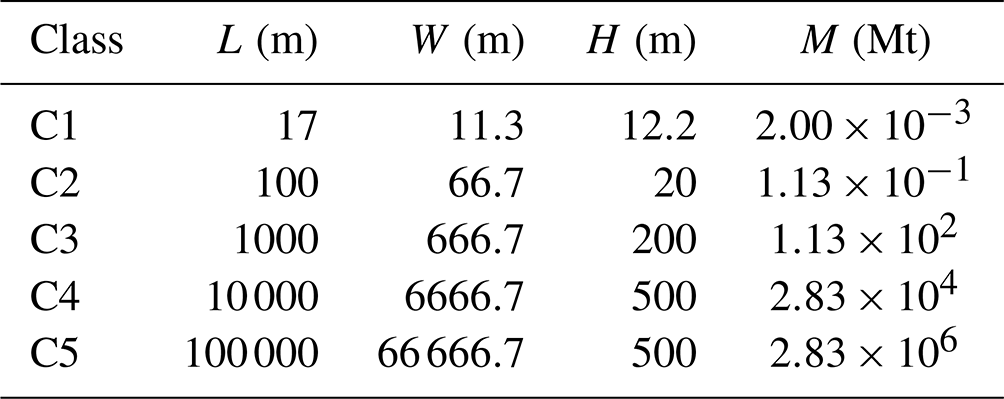
The initial thickness of the icebergs is defined such that $L:H=\mathrm{5}:\mathrm{1}$, which is a common ratio for several iceberg types, including tabular icebergs (Turnbull et al., 2015). However, for the smallest size class (L=10 m), this would give a thickness of 2 m and a draft of only 1.65 m. As the base of the uppermost ocean layer of the model lies at 10.01 m and iceberg motion is only determined by ocean flow, this would remove the basal melt term and hence keep the iceberg thickness static. Therefore, instead, we set the iceberg thickness to 12.2 m (D=10.09 m). Note that this also requires a change in iceberg length to fulfil the tipping criterion explained below.

A second adaptation is required for the maximum iceberg thickness, which is constrained by the thickness of the ice shelf front the berg calved from (England et al., 2020; Gladstone et al., 2001). Whilst most authors use a maximum thickness between 250 and 350 m, related to the average modern ice shelf front thickness (England et al., 2020; Gladstone et al., 2001), here we use a maximum iceberg thickness of 500 m, as the warm Eocene monsoonal climate at the Antarctic coast (Baatsen et al., 2024) could potentially lead to high snow accumulation rates and ample meltwater, creating fast-flowing ice sheets and glaciers with warm bases. In the present day, such ice sheets and glaciers have been found to generate thick icebergs in both Antarctica (Dowdeswell and Bamber, 2007) and Greenland (Dowdeswell et al., 1992). In addition, the present-day Filchner Ice Shelf produces icebergs over 500 m in thickness due to its constrained topographical setting (Dowdeswell and Bamber, 2007) and thus might have done so in the past.

Throughout the duration of the run, the length-to-width ratio of the icebergs is kept constant. The ratio between the iceberg area and thickness, however, changes through the difference in melt rates at the iceberg sides and base. If the width-to-height ratio $W/H$ becomes smaller than a critical value, ε_c, the iceberg capsizes and the iceberg width and thickness are interchanged. Here, ${\mathit{\epsilon }}_{\mathrm{c}}=\sqrt{\mathrm{6}\mathit{\alpha }\left(\mathrm{1}-\mathit{\alpha }\right)}$, where $\mathit{\alpha }={\mathit{\rho }}_{\mathrm{i}}/{\mathit{\rho }}_{\mathrm{o}}$, as adapted by Wagner et al. (2017a) from Weeks and Mellor (1978). Inclusion of this effect can significantly lengthen the lifetime of especially small (L<500 m) icebergs (Wagner et al., 2017a).

2.1.2 Iceberg deterioration

Along its trajectory, the size of an iceberg changes through several processes at both the ice–water and ice–air interface. Following previous literature (e.g. Martin and Adcroft, 2010; Gladstone et al., 2001; Rackow et al., 2017), we limit the included processes in this study to basal melt, buoyant convection, and wave erosion, which are the main contributors to iceberg melting (Bigg et al., 1997) and were found to cause 98 % of the total melt in the Arctic (El-Tahan et al., 1987).

Firstly, turbulence generated by the relative motion of the iceberg in the ambient seawater leads to forced convection or basal melt M_b at the iceberg base (Fig. 2a), which influences the iceberg thickness. This term can be especially important for giant icebergs (Rackow et al., 2017) and, although usually smaller, can reach up to 1 m d⁻¹ (Bigg, 2015) when the difference between the iceberg speed and ocean velocity is particularly large, for example, during iceberg grounding. Secondly, the movement of (warm) ocean water along the submerged sides of the iceberg leads to a heat exchange through buoyant convection M_v (Fig. 2b). This term is usually relatively small, especially in colder areas, with a maximum of roughly 0.2 m d⁻¹ (Cenedese and Straneo, 2023), influencing the horizontal iceberg extent. However, the warmer Eocene ocean might increase the contribution of this term. Thirdly, the impact of waves of relatively warm water causes the iceberg to lose mass around the waterline through wave erosion M_e (Fig. 2c). It can easily reach 1 m d⁻¹, even for small waves (Cenedese and Straneo, 2023), and also influences the horizontal iceberg extent. This melt term often contributes most to iceberg melt and can account for 80 % of the total iceberg deterioration in warmer ocean conditions (Savage, 2001). Thus, it is expected to play a major role in our simulations. A more detailed description of the melt terms, including their formulation, can be found in the previous literature (e.g. Martin and Adcroft, 2010; Merino et al., 2016) and Sect. S2.1.3. However, we will shortly focus on adaptations made here.

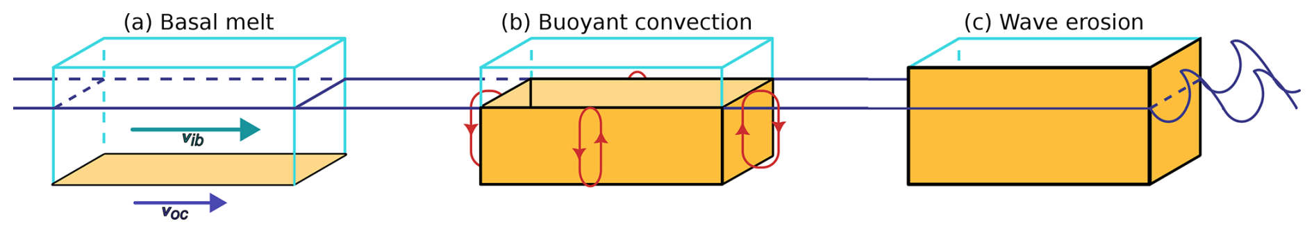
Figure 2 The three processes influencing iceberg deterioration included in the iceberg model. The coloured areas indicate the iceberg areas on which the melt process works. (a) Basal melt is caused by the turbulence generated by the relative motion of the iceberg (v_ib) in the ambient seawater (v_oc). Note that this is the only process affecting the iceberg base. (b) Buoyant convection arises due to the movement of relatively warm ocean water along the submerged iceberg sides. (c) Wave erosion occurs through the impact of relatively warm ocean waves on two iceberg sides.

Although many studies use ocean surface properties to calculate the above melt terms (Martin and Adcroft, 2010; Marsh et al., 2015), we follow Merino et al. (2016) and use depth-integrated values along the iceberg keel. Note that this does not change the parameterisation of wave erosion, as this term depends on the values at the air–sea interface. A second change with respect to much of the previous literature is the adaptation of the internal ice temperature, which is generally set to −4 °C. However, the use of the freezing temperature instead of the internal ice temperature was shown to give better results (FitzMaurice and Stern, 2018). Therefore, we use a value of $T_{\mathrm{f}}=-\mathrm{1.92}$ °C (as derived in Sect. S2.1.3). Finally, iceberg grounding occurs when the iceberg draft exceeds the water depth. In this case, the depth-integrated iceberg velocity is set to zero for the advection (Sect. S2.1.4), inhibiting the iceberg from moving further until it has melted sufficiently during the next time step(s), i.e. when the iceberg draft is smaller than the water depth. Note that this can only be realistically implemented in forward runs (Sect. 2.3).

2.1.3 Notes on the iceberg model

Several choices and assumptions have been made while building the iceberg model. Firstly, the approximation of icebergs as cuboids can lead to an underestimation of melt rates and hence an overestimation of the iceberg lifetimes due to the reduced areas (Hester et al., 2021). In addition, the length-to-width ratios of icebergs are more variable in reality, both through time and at release (Weeks and Mellor, 1978). Still, for most icebergs, the ratio varies between 1:1 and 2:1 (Weeks and Mellor, 1978). In addition, a process similar to basal melting occurs along the submerged iceberg sides (Bigg et al., 1997) and is sometimes also included in models (Rackow et al., 2017). However, as this melt term depends on the friction velocity between the ocean flow along the iceberg keel and the iceberg motion itself, this requires iceberg dynamics not solely dependent on ocean velocity as used in our approach, otherwise the friction velocity will always be zero. Therefore, this melt term was not included in our model.

Most uncertain, however, is the inclusion of wave erosion. The general form of the equation includes a damping term related to sea ice cover (Sect. S2.1.3). Although no direct information on sea ice cover exists in the high-resolution Eocene model used, we can use sea surface temperatures as an indication of the possibility of sea ice formation. Assuming sea ice only forms below −1.8 °C (Baatsen et al., 2020), the Eocene model shows no potential for sea ice formation, as temperatures are constantly higher. We can therefore assume that the dampening effect of sea ice on wave erosion was practically absent. This is also supported by evidence from dinoflagellate cysts suggesting sea ice formation started during the Oligocene (Houben et al., 2013).

Even more important for wave erosion is the representation of the wind. Whilst all other input fields are given at a daily resolution (Sect. 2.2), we have to restore to monthly wind stress fields, as no wind velocity fields are available, and neither exists on a daily resolution. Comparison using high- and low-resolution temporal data of the present day shows this leads to an average difference in wave erosion of 31 % (Sects. 4.4 and S3.1.4). Hence, we expect wave erosion melt rates in this study to be underestimated.

Finally, more general exclusions from the model are the computation of weighted means when icebergs extend through multiple grid cells (Rackow et al., 2017) and the parameterisation of iceberg breakup. Exclusion of the latter has been found to overestimate iceberg lifetimes compared to observations (England et al., 2020), and iceberg breakup in open waters can cause up to 80 % of the total iceberg mass loss of large icebergs at present (Tournadre et al., 2015). To avoid this problem, Wagner et al. (2017b) removed such large icebergs from the model run after 1 year, although this leads to an underestimation of the icebergs' lifetime, as they would not necessarily have disappeared after 1 year in reality. As such, we do not remove large icebergs from the model but need to keep in mind that their lifetime is likely to be overestimated.

2.2 Eddy-resolving ocean model

The simulations in this study are performed using the high-resolution eddy-resolving model of the late Eocene by Nooteboom et al. (2022). This ocean-only Parallel Ocean Program (POP) model (Smith et al., 2010) has a horizontal resolution of 0.1°, which allows it to include smaller-scale structures such as ocean eddies. It is forced at the surface by a fixed atmosphere of the fully coupled simulations of the Community Earth System Model, or CESM, version 1.0.5 (Baatsen et al., 2020) under a 2× preindustrial CO₂ forcing to simulate the late Eocene. The bathymetry of CESM was interpolated linearly to the high-resolution POP grid.

As required for the iceberg melt calculations, multiple fields up to 730 m depth were used, covering a 5-year time span (model years 38 to 42) at a daily resolution. These include the 3D ocean horizontal ocean velocity component (Fig. 1b) and 3D temperature (Fig. 1b) fields. In addition, for the same model years (albeit on a monthly resolution), the horizontal surface wind stress components were used to approximate wind velocity, as the latter was not available from the model.

Although the high resolution of this model allowed a more accurate simulation of palaeotemperatures and circulation (Nooteboom et al., 2022), we need to keep in mind that the model has no dynamic ice component and thus does not account for a regional ice-induced cooling (Manabe and Broccoli, 1985). Therefore, if ice were present in Antarctica during the late Eocene, ocean temperatures in the vicinity of these ice masses might have been slightly lower than projected. Although this effect is likely minor, as the currently projected temperatures are vastly above zero, it might have made iceberg survival somewhat more realistic.

2.3 Locations and regions

Several locations and regions were defined in constructing this model. Firstly, we need to determine the palaeolocation of ODP Site 696 during the late Eocene. Although presently located at 61°50.959^′ S, 42°55.996^′ W on the southeastern margin of the SOM at 650 m water depth, palaeo-oceanographic reconstructions (López-Quirós et al., 2021) and visual comparison of the present-day and Eocene bathymetry places the palaeolocation of ODP Site 696 around 67°5^′ S, 57° W (Fig. 1) in a shallow-water environment at roughly 250 m palaeo-depth. During the simulations, we assume icebergs coming within the distance of 1 grid cell (∼ 11 km) to be able to deposit IRD at the site unless otherwise indicated. While this range can be considered to be quite conservative, especially for the larger size classes which extend through multiple grid cells, this narrow range allows a consistent method that can be applied for all iceberg sizes without taking into account their actual size in the vicinity of ODP Site 696 and reduces the risk of overestimating the number of icebergs reaching the site by accounting for uncertainties in the trajectories.

Secondly, two sets of iceberg release locations were defined. Using the analysis of the relation between the hinterland geology and the IRD by Carter et al. (2017) as a guideline, we spread 25 locations at the 500 m bathymetry line with a longitudinal spacing of 2° between the coast offshore the Ellsworth Mountains and Dronning Maud Land (24 points) and a 5° longitudinal spacing along the Antarctic Peninsula (1 point; Fig. 1) to test where icebergs released along the Antarctic coast end up. The coastline was further divided into six regions following the division by Carter et al. (2017), but note that we exclude northern Graham Land as the bedrock here was shown to be too young compared to the IRD found at ODP Site 696 (Carter et al., 2017). In addition, we include Palmer Land and the eastern sector of Dronning Maud Land, which were not included in the analysis of Carter et al. (2017). During backward simulations, for which 25 locations were defined within the grid cell around ODP Site 696 (Fig. 1), these regions were used to locate possible source regions of IRD for icebergs reaching ODP Site 696.

2.4 Experimental design

In order to test whether icebergs from the southern Weddell Sea region can indeed reach ODP Site 696 as suggested by Carter et al. (2017), we set up 11 different simulations.

Firstly, forward runs (i.e. runs with iceberg releases at the Antarctic Margin forward in time to see where they end up) with grounding are performed for all five size classes (Table 1). In addition, the sensitivity of these runs to various conditions is tested by studying the effect on icebergs of class C4. This is performed by (1) including icebergs within 2 grid cells' distance to ODP Site 696 (∼ 22 km) and (2) executing the model using only surface fields instead of depth-integrated values as is usually done in iceberg models (e.g. Bigg et al., 1997; Gladstone et al., 2001; Martin and Adcroft, 2010).

In addition to these seven forward runs, we set up four backward simulations. During these simulations, we calculate the iceberg trajectories backwards in time away from ODP Site 696 towards Antarctica by calculating iceberg growth through reverse melting. These simulations are performed by releasing icebergs of the three smallest size classes from ODP Site 696, since we expect icebergs to be relatively small once reaching ODP Site 696 under the influence of the high late Eocene temperatures. In addition, as for the forward simulations, a simulation using only surface fields is performed for size class C1. Note that none of these scenarios include iceberg grounding, as information on the duration an iceberg was grounded at a certain position is lost in backward time.

For each scenario, icebergs are released daily at all respective release locations for the 5-year model period, leading to 1823 releases per site. Sampling is performed at an hourly interval in order to satisfy the Courant–Friedrichs–Lewy (CFL) condition and avoid overshooting cells during advection. Note that the IRD found at ODP Site 696 does not provide information on the number of icebergs that have reached the site, and, as such, we are interested in the possibility that any iceberg reaches ODP Site 696 from the defined release locations during the simulations. Still, of course, a larger number of icebergs able to reach ODP Site 696 would increase the likelihood of any icebergs reaching the site.

3 Results

We first study the forward trajectories to analyse if icebergs can reach ODP Site 696 for any of the iceberg size classes. From this, we can infer possible source locations of IRD. Next, by studying the backward trajectories, we can determine the minimum iceberg size required at each calving site. Finally, the sensitivity of the model to various settings is analysed.

3.1 Flow patterns and iceberg trajectories

Irrespective of the simulation, most icebergs seem unable to reach ODP Site 696 (Fig. 3). From the two smallest size classes (not shown), none of the icebergs arrived at ODP Site 696. The same holds for size class C3, although, in this case, some icebergs can at least reach the northern part of the Antarctic Peninsula. For size class C4, release locations west of Gunnerus Ridge are (at least in some cases) able to generate icebergs that can reach ODP Site 696. These trajectories will be referred to as “successful” in the rest of the text. For C5, interestingly, none of the icebergs seem able to reach ODP Site 696. However, note that some of the trajectories do seem to pass close to ODP Site 696 visually, so using a wider range to select icebergs reaching ODP Site 696 would likely increase the number of successful icebergs in these simulations.

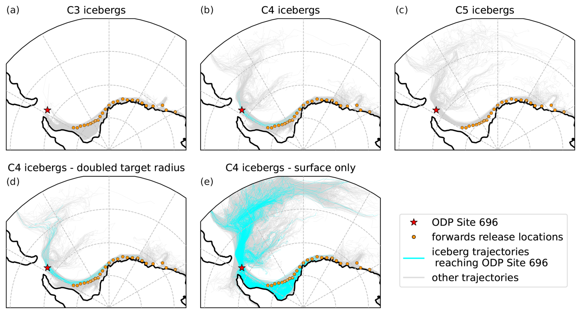
Figure 3 Iceberg trajectories from forward simulations that can (blue) or cannot (grey) reach ODP Site 696 within the distance of 1 grid cell (∼11 km) at some point along their trajectory. (a, b, c) Results of the main simulations run for iceberg size classes C3, C4, and C5. (d, e) Results of the sensitivity simulations run for iceberg size class C4 with the inclusion of icebergs passing ODP Site 696 at twice the distance of a grid cell (d) or when using only surface fields (e). The trajectories of size classes C1 and C2 are not shown, as none of these trajectories reach near to ODP Site 696. Note that the marker of ODP Site 696 is roughly half the size of the SOM.

Some general information can also be gleaned from the complete set of trajectories. In all three scenarios shown in the top row of Fig. 3, icebergs initially seem to travel relatively close to the coast in an anticlockwise direction. However, for the smaller icebergs of class C3, icebergs are able to flow far onto the Ronne–Filchner Ice Shelf and over the interior of Gunnerus Ridge. In class C4, these regions are only sparsely crossed by icebergs, and, for size class C5, they are nearly devoid of trajectories. Moreover, the presence of Gunnerus Ridge seems to induce relatively chaotic patterns in the iceberg trajectories in the vicinity of this region.

After reaching the tip of the Antarctic Peninsula, icebergs head in several general directions. Firstly, icebergs can travel northeastwards. For C3, however, most icebergs seem to have melted completely before crossing 65° S. For size class C4 and especially C5, icebergs can survive longer and are able to leave the domain shown here northwards or in some cases float eastwards around 67° S. A second route possible after leaving the Antarctic Peninsula starts in the southeastern direction and continues with icebergs heading either northeastward or circling back towards the Antarctic coast.

3.2 IRD provenance

To study in more detail where the icebergs reaching ODP Site 696 might have been derived from, we now focus on the percentage of releases from each forward release location that crosses over ODP Site 696 at some point during its trajectory (Fig. 4). As indicated before, none of the release locations lead to successful releases for the smallest three iceberg size classes. For size class C4, however, icebergs can reach ODP Site 696 from several locations along the Antarctic coast. This includes Palmer Land (locations 1 and 2), offshore the Filchner Ice Shelf (locations 5, 7, and 8), and even western and eastern Dronning Maud Land (locations 13, 15, and 21). For even larger icebergs, no successful trajectories exist. Note that, as such, irrespective of iceberg size, none of the icebergs released offshore the Ellsworth Mountains and Coats Land or in the eastern part of Dronning Maud Land east of Gunnerus Ridge are able to reach ODP Site 696 for the main simulations.

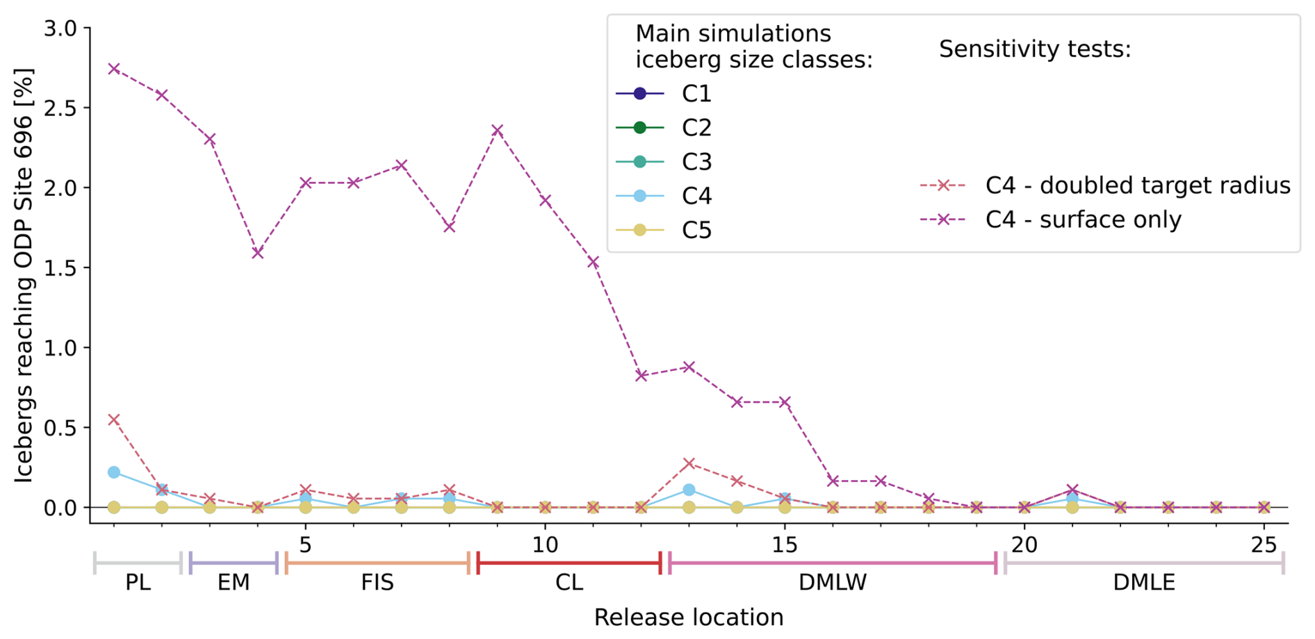
Figure 4 Percentage of total releases per forward release location (Fig. 1) that reach ODP Site 696 at some point along their trajectory. Solid lines denote the main forward simulations for each iceberg size class. Dashed lines show the sensitivity simulations of size class C4 when including icebergs passing ODP Site 696 at twice the distance of a grid cell (“doubled target radius”) or when using only surface fields (“surface only”). The coastal regions based on Carter et al. (2017) (Fig. 1) are indicated on the x axis, where PL is Palmer Land, EM is the Ellsworth Mountains, FIS is the Filchner Ice Shelf, CL is Coats Land, and DML is Dronning Maud Land (W: west; E: east). The total number and percentage of releases reaching ODP Site 696 per simulation are given in Table A1 (Appendix A). Note that the lines of the smaller iceberg classes (C1–C3) are overplotted and are zero everywhere.

3.3 Minimum iceberg size

Next, by backtracking icebergs from ODP Site 696 to the Antarctic coast (i.e. releasing icebergs at ODP Site 696 and following their backward-in-time trajectory and reverse melting towards the Antarctic coast), we obtain a first indication of the minimum iceberg size required at different locations along the Antarctic coast. Firstly, the results are described spatially to visualise the extent of potential iceberg origins. Then, the results are analysed per defined region to give a clearer view of the most probable minimum and maximum iceberg size per region.

3.3.1 Spatial patterns

The spatial patterns of iceberg mass (Fig. 5a) and thickness (Fig. 5b) clearly show that, irrespective of the size class, iceberg size generally increases with alongshore distance to ODP Site 696. As could be expected, the exact sizes differ strongly between the size classes, reaching values of over 600 Mt for C1, 1000 Mt for C2, and over 15 000 Mt for C3. In terms of thickness, icebergs range between roughly 15 and 26 m for class C1, 23 and 35 m for class C2, and 205 to 235 m for class C3. Interestingly, it seems that the icebergs reaching the region around Gunnerus Ridge are relatively small; that is to say, icebergs here can be smaller or comparable to those reaching the western part of Dronning Maud Land.

A second feature evident from Fig. 5a and b is that, while the spatial extent of icebergs from classes C1 and C2 is quite similar, icebergs of class C3 can reach a larger part of the Antarctic coast. For class C1 and C2, icebergs reach more or less continuously to 15° E and only sporadically further into Dronning Maud Land in the vicinity of Gunnerus Ridge. In both cases, icebergs appear generally unable to reach the southeastern part of the Filchner Ice Shelf and a small patch in front of Coats Land. For C3, coverage is broader and extends until Gunnerus Ridge. Notably, in all three experiments, icebergs can reach the region eastward of Gunnerus Ridge, which did not seem possible in the forward experiment.

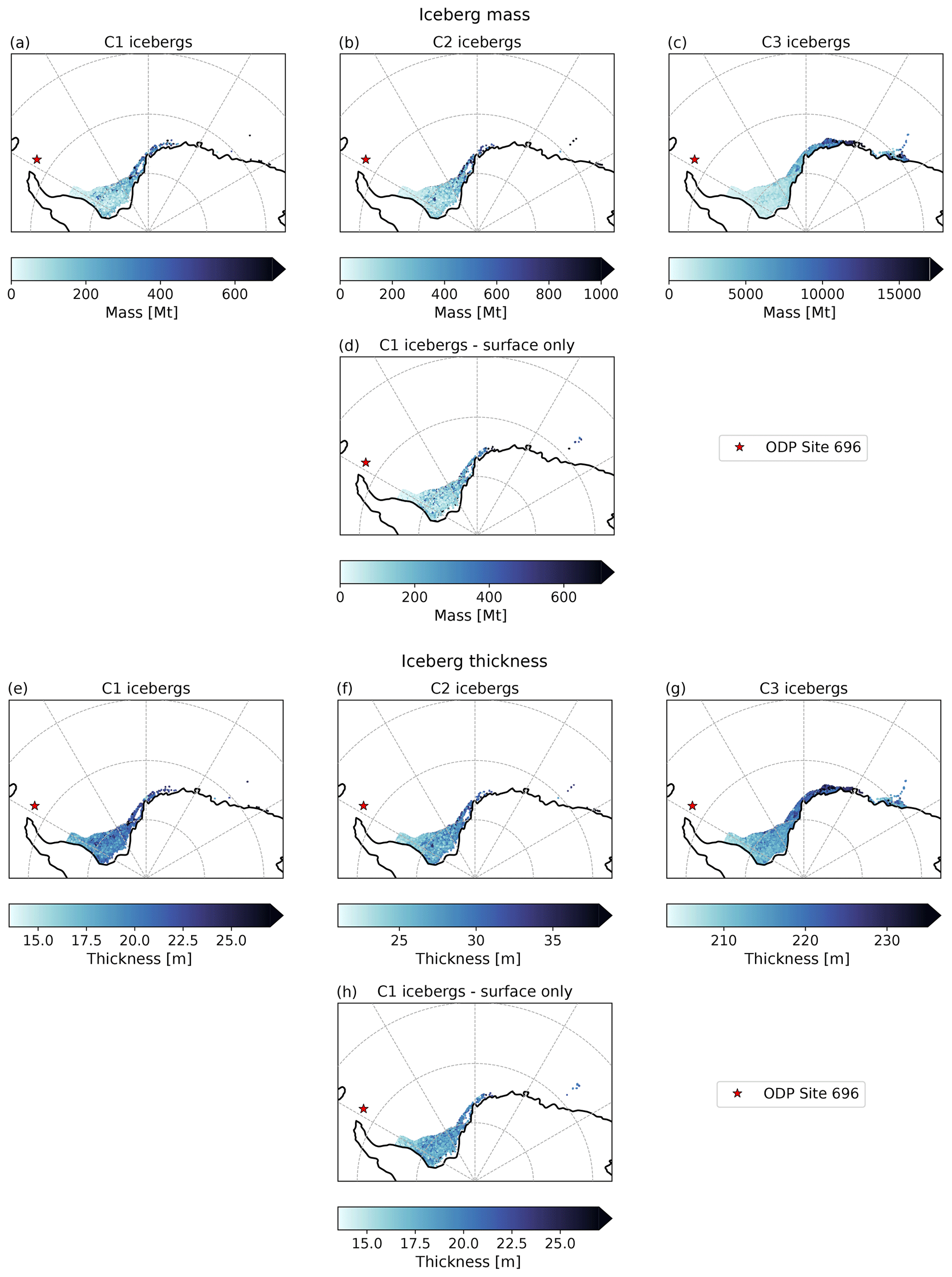
Figure 5 Spatial mass and thickness distributions obtained with backward simulations for (a–d) iceberg mass and (e–h) iceberg thickness within the defined coastal region of the southern Weddell Sea based on Carter et al. (2017) (Fig. 1). (a–c, e–g) Results of the main backward simulations run for iceberg size classes C1, C2, and C3. (d, h) Results of the sensitivity simulation for iceberg size class C1 using only surface fields. The total number of data points per simulation are given in Table B1 (Appendix B). Note that the marker of ODP Site 696 is roughly one-quarter of the size of the SOM.

3.3.2 Regional patterns

Turning now to the distribution of iceberg mass (Fig. 6a) and thickness (Fig. 6b) within each coastal region reveals several things. As was apparent in the figures above, both the mass and the thickness with the highest probability generally show an alongshore increase through the coastal regions – independent of the initial iceberg size class. The same typically holds for the minimum and maximum values in these regions but not for the outliers. In addition, the range of probable values of iceberg mass typically increases from Palmer Land to Dronning Maud Land. Again, the order of iceberg size varies between the different size classes. For C1, icebergs able to reach the coast have a mass on the order of 10⁻¹ to 10³ Mt and a thickness of (a few) tens of metres. The range is similar for size class C2 but with the upper limit of iceberg thickness now extended to just above 100 m. For class C3, iceberg mass is on the order of 10² to 10³ Mt, with iceberg thicknesses on the order of 10² m.

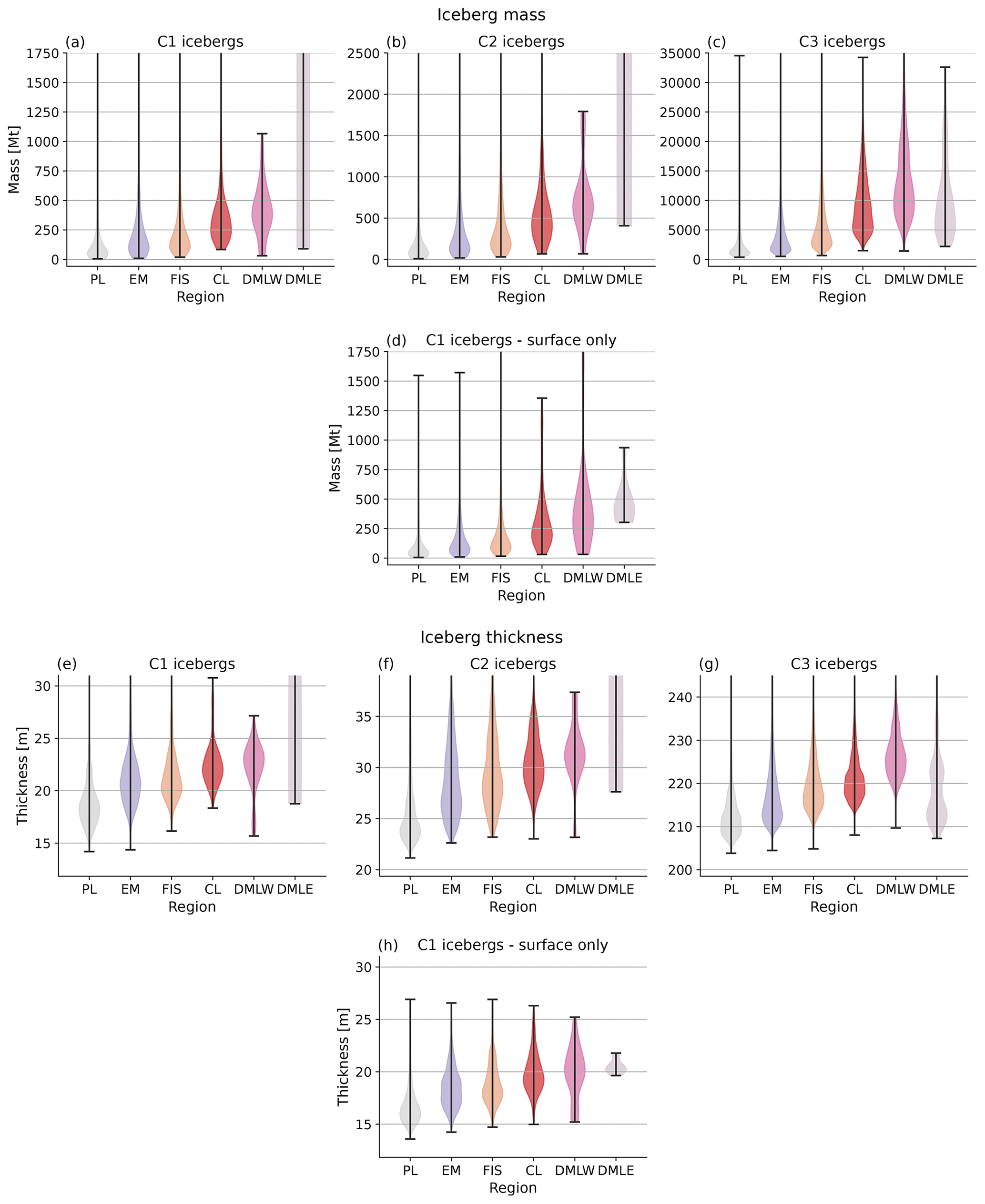
Figure 6 Visualisation (violin plot) of the mass and thickness distributions obtained with backward simulations for the (a–d) minimum iceberg mass and (e–h) minimum iceberg thickness in each coastal region (Fig. 1), where PL is Palmer Land, EM is the Ellsworth Mountains, FIS is the Filchner Ice Shelf, CL is Coats Land, and DML is Dronning Maud Land (W: west; E: east). (a–c, e–g) Results of the main backward simulations run for iceberg size classes C1, C2, and C3. (d, h) Results of the sensitivity simulation run for size class C1 when using only surface fields. The number of data points per region are given in Table B1 (Appendix B), and the full range of possible values is shown in Fig. C1 (Appendix C).

Going through the size classes one by one, starting at C1, shows a most probable mass of around 50 Mt in Palmer Land, increasing to roughly 400 Mt in the western sector of Dronning Maud Land. In the eastern sector of Dronning Maud Land, iceberg mass is highly variable, with probable values of iceberg mass ranging from around 150 to over 40 000 Mt. Interestingly, the range of the minimum iceberg mass observed in the western sector of Dronning Maud Land, including outliers, is smaller than that in any of the other regions and, excluding the western sector of Dronning Maud land, largest in the most proximal region (Palmer Land). Finally, the minimum size observed in Coats Land is larger than that in the more distant western sector of Dronning Maud Land.

For size class C2, overall similar patterns are found with icebergs ranging from just below 10 Mt in Palmer Land to over 50 000 Mt in the eastern sector of Dronning Maud Land. Icebergs of size class C3, on the other hand, show some interesting differences. Firstly, the iceberg mass in the eastern sector of Dronning Maud Land is now not only much more constrained and closer to that of the other regions (between roughly 2500 and 25 000 Mt), but the most probable mass (around 5000 Mt) is lower than that in the western sector of Dronning Maud Land (10 000 Mt). Moreover, the minimum mass (excluding outliers) in the eastern sector of Dronning Maud Land is smaller than that in the western sector (2500 compared to 4000 Mt).

Finally, as was stated before, similar trends are observed in iceberg thickness. However, in addition, Fig. 6b shows that the difference in the most probable minimum iceberg thickness between adjacent regions is within roughly 3 m for C1, 4 m for C2, and 10 m for C3. Generally, the difference in thickness between the same region for C1 and C2 varies between 6 to 8 m and between roughly 185 and 195 m between C2 and C3. In all three cases, the thickness of icebergs in the eastern sector of Dronning Maud Land shows a (slightly) bimodal pattern. For C1 and C2, respective dominant thicknesses lie around 20 and 90 or 30 and 110 m. For class C3, the probabilities are highest around 212 and 222 m. For none of the simulations does the maximum iceberg thickness, including outliers, extend above 260 m.

3.4 Model sensitivity

Finally, we are interested in the sensitivity of the model to several variables.

3.4.1 Doubled target radius

Including icebergs reaching within the distance of two grid cells from ODP Site 696 increases the number of successful trajectories (Fig. 3). Specifically, whilst for the regular simulation 0.029 % of the trajectories was successful, doubling the allowed distance increases this to 0.66 % (Table A1 in Appendix A). This increase is for two reasons. Firstly, several sites previously not releasing any icebergs to ODP Site 696 are now viable release locations (e.g. locations 3, 6, and 14). Secondly, in addition to more sites contributing, already successful locations release more icebergs to ODP Site 696, which is especially notable for release locations 1 and 13 (Fig. 4).

3.4.2 Surface fields

Using only surface fields during the simulation for icebergs of size class C4 leads not only to a significant increase in the number of icebergs reaching ODP Site 696 (Fig. 4) but also to a changed pattern of trajectories (Fig. 3) compared to the simulation using depth-integrated fields. Icebergs now seem able to travel over the shallower regions along the Antarctic Coast, such as the Ronne–Filchner Ice Shelf. In addition, some icebergs traverse westwards through the Drake Passage and more icebergs appear to travel eastward around 57° S. Nevertheless, icebergs released from locations 19, 20, and 22 to 25 in Dronning Maud Land still appear unable to reach ODP Site 696.

Using only surface fields during backward simulations for size class C1 shows relatively similar results in terms of iceberg mass (Fig. 6a). In the eastern sector of Dronning Maud Land, however, the iceberg mass is now much more constricted, never reaching above 1000 Mt. In all regions except the eastern part of Dronning Maud Land, the most probable iceberg thickness is roughly 2.5 m smaller compared to the depth-integrated simulations (Fig. 6b). As for the iceberg mass, the iceberg thickness in the eastern part of Dronning Maud Land is more constricted, varying between roughly 20 and 22 m.

4 Discussion

4.1 Flow patterns and iceberg trajectories

An important factor in determining whether Antarctic icebergs could reach ODP Site 696 during the late Eocene, as suggested by Carter et al. (2017), is the pattern of ocean currents. A broad comparison of the high-resolution Eocene model (Nooteboom et al., 2022) to present-day fields (Mercator Ocean International (Gasparin et al., 2018) and ECMWF ERA5 reanalysis data (Hersbach et al., 2023); see Sects. S2.1.2 and S3.1.4) shows that, while the surface ocean velocities in general are of the same order (up to ∼ 0.4 m s⁻¹), the ocean patterns differ. While the present-day ACC is clearly visible as a continuous meandering structure, the late Eocene proto-ACC shows more eddying behaviour and latitudinal variation (Fig. D1a, Appendix D). Indeed, as the ocean gateways around Antarctica had not yet fully opened and deepened at the end of the Eocene (, 2015), the ACC was not fully developed at this time (Hill et al., 2013; Evangelinos et al., 2024).

More important to the iceberg trajectories in the Weddell Sea at present is the presence of the Antarctic Coastal Current (ACoC), as most icebergs released along the Antarctic coast flow with the anticlockwise ACoC until meeting the ACC in the Scotia Sea (Weber et al., 2021), a region colloquially called “Iceberg Alley”. From both the late Eocene trajectories (Fig. 3) and the mean current patterns themselves (Fig. S4.1, Sect. S4), we can deduce that a similar current existed along the coast of the Antarctic Peninsula during the late Eocene – although a persistent westward alongshore branch of the ACoC does not seem to exist yet. The presence of a proto-ACoC is also supported by other palaeo-oceanographic studies of the Eocene (Huber et al., 2004; Bijl et al., 2011; Sauermilch et al., 2021). In that regard, the position of ODP Site 696 seems to have been in a location similar to the present-day Iceberg Alley and, as such, was potentially ideally placed for passing icebergs, if present.

Finally, while the present-day circulation shows dominantly offshore currents that turn eastward with decreasing latitude (Fig. D1c, Appendix D), due to the presence of the ACC, the direction of flow in the Eocene is much more chaotic (Fig. E1a, Appendix E), thus potentially hindering fast iceberg transport towards ODP Site 696. Similarly, while the present-day winds consist of dominantly offshore katabatic winds (e.g. Parish and Bromwich, 1991), the Eocene model shows offshore winds persisting in the western Weddell Sea but onshore winds dominating along the coast of Dronning Maud Land (Fig. E1b, Appendix E). As the effect of wind drag is ignored in our model, this does not strongly affect the iceberg trajectories but does suggest that taking wind drag into account could lead to an increase in iceberg speed where the ocean flow and winds align.

4.2 IRD provenance

IRD provenance between Palmer Land and Dronning Maud Land seems possible – albeit sporadically (Fig. 4). Firstly, our simulations show that trajectories from Palmer Land could reach ODP Site 696, making this a potential source of IRD. Unfortunately, bedrock samples from this region were not taken into account during the analysis by Carter et al. (2017). However, based on the recently constructed geological map of Antarctica (GeoMAP) (Cox et al., 2023), the mountainous region of Palmer Land is given an approximately Jurassic to Cretaceous age (200–66 Ma), giving it a roughly similar age to northern Graham Land, the region in the northernmost part of the Antarctic Peninsula. Since sediments of the latter region were found to be relatively dissimilar to those found at ODP Site 696 (Carter et al., 2017), we infer it is unlikely that icebergs from Palmer Land brought IRD to this site.

To study this further, we can compare these locations to regions of potential glacial formation during the late Eocene, such as from simulations by Baatsen et al. (2024), who simulated late Eocene Antarctic climate regimes using several climate indices, and Van Breedam et al. (2022), who used a coupled ice sheet–climate model to study late Eocene glaciations. Although the extent of glaciation inland differs significantly between these studies, their projected near-coastal glaciated regions match well. Generally, these studies show that regions at high altitudes and near the coast are likely locations of glacial formation, as these regions are often characterised by lower temperatures, high precipitation rates, or both. Indeed, glaciation is suggested in the higher-altitude regions of Palmer Land (Baatsen et al., 2024; Van Breedam et al., 2022). However, these glaciers were probably restricted to the higher-altitude regions and were not marine-terminating, hence inhibiting iceberg production.

A glacial regime is also suggested along the coast between the Ellsworth Mountain and Filchner Ice Shelf regions (Baatsen et al., 2024; Van Breedam et al., 2022). From the main simulations, however, no successful trajectories arise from the Ellsworth Mountain region, and only icebergs of size class C4 can reach ODP Site 696 from offshore the Filchner Ice Shelf. Bedrock samples from this region were also shown to be in good accordance with the provenance of the IRD found at ODP Site 696 (Carter et al., 2017), suggesting this region could be a likely source of the IRD. Whilst rocks from the shelf region of Coats Land also showed significant similarities to the provenance of the IRD, no successful trajectories in the main simulations exist for these sites. In addition, neither Baatsen et al. (2024) nor Van Breedam et al. (2022) suggest glacial conditions in this region. Hence, we can exclude this region as a potential source of IRD.

Finally, icebergs released along Dronning Maud Land can reach ODP Site 696 in our simulations. Although only the western sector was included in the analysis by Carter et al. (2017), both sectors have a similar geology (Cox et al., 2023) and, as such, are a potential source of IRD. In addition, the section between roughly 10 and 50° E is shown to have a glacial regime (Baatsen et al., 2024; Van Breedam et al., 2022). However, depending on the simulation, glacial formation is limited to the slightly inland high-altitude region only, suggesting it might not have been possible to form marine-terminating glaciers. Still, we cannot exclude the presence of marine-terminating glaciers; hence, under the right circumstances, it might have been possible for icebergs released along the Dronning Maud Land coast to deposit IRD at ODP Site 696 at the SOM.

It is also worth noting that, while our study focuses on Antarctic icebergs reaching ODP Site 696 based on the results of Carter et al. (2017), it seems reasonable to assume that IRD could have been deposited in a wider area surrounding this site during the late Eocene. For example, as can be seen from the trajectories in Fig. 3, many trajectories seem to visually reach ODP Site 696 but fall outside the used target radius. As also suggested by the sensitivity simulation with a doubled target radius, increasing this radius even more might lead to a further increase in the number of successful trajectories. In turn, this might allow iceberg trajectories from the Ellsworth Mountains region, which was suggested to have a glacial regime (Baatsen et al., 2024; Van Breedam et al., 2022) but did not provide any successful trajectories with the current target radii used, to be counted as successful.

Finally, in addition to the regions discussed above, one could argue that it might have been possible for icebergs released west of the Drake Passage to reach ODP Site 696 based on the position of the South Orkney Microcontinent at the tip of the Antarctic Peninsula during the late Eocene. Indeed, modelling studies suggest a potential for glacial conditions around 150° W in Marie Byrd Land and at several points along the (western) Ross Sea (Baatsen et al., 2024; Van Breedam et al., 2022). However, Marie Byrd Land consists predominantly of rocks of Devonian age and younger (< 420 Ma) and, as such, is an unlikely source of the IRD. Whilst the ages of the bedrock found along the western Ross Sea extend until the Neoproterozoic, no samples older than 760 Ma have been found; hence the older part of the age distribution found at ODP Site 696 seems to be absent here too. We thus adhere to the coastal regions defined by Carter et al. (2017) based on the hinterland geology.

To summarise, the simulated trajectories suggest icebergs released along the coasts from Palmer Land to Dronning Maud Land can potentially deposit IRD at ODP Site 696, except for the regions offshore the Ellsworth Mountains and the Coats Land shelf. However, taking into account potential regions of glacial formation (Baatsen et al., 2024; Van Breedam et al., 2022) and the local geology (Cox et al., 2023; Carter et al., 2017), the regions offshore the Filchner Ice Shelf and Dronning Maud Land are the most likely source locations of the IRD found at ODP Site 696.

4.3 Minimum iceberg size

Having constrained the potential regions from which icebergs could have been released to ODP Site 696 at the SOM, this section aims to determine the minimum required iceberg size along these stretches of coast and to analyse the feasibility of these sizes.

From the backward simulations starting with icebergs in size class C1, we find that the minimum probable iceberg mass and thickness offshore the Filchner Ice Shelf are around 20 Mt and 18 m. The most probable iceberg size in this region is roughly 125 Mt and 20 m. For Dronning Maud Land, the minimum iceberg mass (thickness) following from the simulations is 30 or 90 Mt and 20 or 19 m, respectively, with the most probable size roughly 375 or 45 000 Mt and 23 or 88 m.

When starting the backtracking with larger icebergs (class C2), the minimum iceberg mass (thickness) increases to 30 (23.5) offshore the Filchner Ice Shelf, 150 (28) in the western sector of Dronning Maud Land, and 400 Mt and 27.5 m in the eastern sector of Dronning Maud Land. The most probable minimum size in each region is roughly 250, 700, or 45 000 Mt and 27.5, 31.5, or 100 m. Finally, for icebergs released as size class C3, icebergs originating from offshore the Filchner Ice Shelf should have a mass (thickness) of at least 900 Mt (211 m), from the western sector of Dronning Maud Land 4000 Mt (218 m) and from the eastern sector 2250 Mt (208 m). Most probable, however, are icebergs with a mass (thickness) of roughly 2500 (215), 9000 (225), or 5000 Mt (212 m). In all cases, the sizes obtained at the coast lie roughly above size classes C3 and larger. However, the change in thickness of especially the smallest icebergs seems relatively minor throughout these simulations, which is related to the low occurrence of tipping. As tipping is related to the width-to-height ratio of the iceberg (Sect. 2.1.1), the on average higher melt rates impacting the growth of the horizontal dimensions of the iceberg in the warm ocean during backward simulations – particularly through high wave erosion rates – compared to the melt rates impacting the growth of the vertical dimension (basal melt) lead to a relatively stable iceberg throughout the simulation. In these simulations, the change in iceberg thickness is thus mostly due to the accumulated effect of basal melt through time. However, the effect of this on the iceberg trajectory was found to be minor.

In addition to the information on iceberg size gathered from backward simulations, the forward simulations can also provide an estimate on the order of magnitudes possible. These simulations showed that, when icebergs are too small at release from the coast (size class C1, C2, or C3), they cannot reach ODP Site 696. While icebergs of class C3 do visually pass near ODP Site 696 and might thus be successful with a less conservative target radius, icebergs of class C1 and C2 melt away long before approaching ODP Site 696. Note that this reduces the importance of the potential deviation in their trajectories by the exclusion of wind drag.

Only icebergs of size class C4 were able to reach this site from offshore the Filchner Ice Shelf and Dronning Maud Land. Moreover, when icebergs grow too large (C5), they are unable to reach the site due to interactions with the bathymetry and changes in their trajectories (Fig. F1, Appendix F), resulting in a lower number of successful trajectories than for class C4 (Figs. 3 and 4). In this case, apparently, the icebergs cannot melt fast enough to enter water depths around 250 m – which is the approximate depth of ODP Site 696 during the Eocene. Consequently, the forward simulations suggest icebergs should be around size class C4 upon release at the coast.

Before delving more into the magnitude of the iceberg sizes obtained, we first examine the wide range of probable iceberg sizes obtained in the eastern sector of Dronning Maud Land for classes C1 and C2 (Fig. C1 in Appendix C). For all three size classes from the backward simulations, the relative difference in the minimum mass or thickness in the eastern sector of Dronning Maud Land between the other regions is in a similar range. However, the maximum probable size lies far outside the range of observed sizes, including outliers, for class C1 and C2 but seems still within range for class C3. A possible explanation for this might be that there are only a few data points in the eastern sector of Dronning Maud Land (Table B1 in Appendix B), skewing the results to values that might otherwise have been considered outliers. As is visible in Fig. C1 (Appendix C), the distribution in this region also does not contain outliers. Of course, while this could explain the relatively large probable values, it does not explain why such large sizes occur in the first place. This is due to iceberg trajectories that circulate through the Weddell Sea and nearby regions for a long time before eventually reaching the Antarctic coast, consequently allowing them to acquire a sizeable mass.

Returning to the obtained iceberg sizes to analyse whether they are realistic, we start by comparing them to present-day (Antarctic) calving-size distributions, such as those of Stern et al. (2016), who define 10 size classes based on observations. This shows that the minimum iceberg sizes found in this study are on the larger end of regularly found iceberg sizes of the present day, falling into size classes 7 and larger. In addition, one needs to take into account that the backward simulations give an estimate of iceberg size on the lower side as, for example, grounding has not been taken into account. Hence, it is likely that icebergs would have needed to be larger, falling into even larger size classes to the present-day distribution. Note, however, that icebergs larger than class 10 do exist at present but are considered to calve more infrequently. Specifically, the calving-size distribution by Stern et al. (2016) uses icebergs that are small compared to the icebergs observed around Antarctica at present. This is because Stern et al. (2016) build on Gladstone et al. (2001) and Bigg et al. (1997) and originally base their melt model on the smaller Arctic icebergs.

To analyse the upper off-scale end of the iceberg classes in more detail, we can compare the obtained iceberg sizes to some of the largest icebergs observed. These include Iceberg B-15 calved from the Ross Ice Shelf, the largest iceberg observed by satellites with an estimated mass of several 10⁵ Mt (Martin et al., 2007), and Iceberg A-68 calved from the Larsen C Ice Shelf with a mass of roughly 10⁶ Mt (Benn and Åström, 2018). It is thus possible at present to form icebergs larger than the minimum sizes suggested by the late Eocene simulations. Nonetheless, such calving events are infrequent and occur at floating ice shelves (Stern et al., 2016). As the late Eocene ocean and air temperatures were relatively warm around Antarctica, it could be argued that the formation of (large) ice shelves would have been unlikely, as recent and future warming are shown to cause thinning and retreat of ice shelves (Meredith et al., 2022). Indeed, the Eocene forcing model assumed no ice was present on Antarctica during the warm Eocene for these simulations. If, however, ice was present in late Eocene Antarctica, atmospheric and oceanic conditions might have been different locally, and, as such, temperatures might currently be overestimated by the model. Hence, the potential for the formation of glaciers, icebergs, and floating ice shelves might be underestimated from the current model.

Finally, the collapse of an ice shelf under high temperatures could lead to the release of several (large) icebergs, such as during Heinrich events (Marcott et al., 2011; Hulbe et al., 2004) and, more recently, for the Larsen B Ice Shelf (Cook and Vaughan, 2010). However, as stated before, such large icebergs were likely unable to reach ODP Site 696, as their size would prohibit them from reaching over the shallow regions of the SOM.

In summary, the simulations here suggest icebergs should have been between at least size classes C3 and C4 when released offshore the Filchner Ice shelf and Dronning Maud Land regions in order to be able to reach ODP Site 696. Compared to present-day iceberg distributions, these icebergs would be on the larger end of the range but not unfeasible, as the high Eocene snow accumulation rates could have allowed a fast discharge of ice towards the coast, hence increasing iceberg calving.

4.4 Iceberg melt rates

Although ocean circulation plays an important role in determining whether icebergs could reach ODP Site 696 in terms of connectivity, the iceberg melt rates influence these trajectories and determine whether icebergs can survive long enough to travel the required distance to the site. For a first impression of iceberg melt rates, we can study the half-life of the icebergs. In general, iceberg lifetime decreases with size. For the present day, icebergs up to L=1000 m (size class C3 in our study) were found to have a half-life between 2 and 5 years in the colder waters in the proximity of the Antarctic coast and 1 year once entering warmer waters (Orheim et al., 2023), as cited in Wesche and Dierking (2014). Larger icebergs can have lifetimes up to several decades, depending on their size and the waters they drift through (Wesche and Dierking, 2014).

As temperatures in the late Eocene were much higher even at the Antarctic coast, reaching temperatures around 10 °C (Fig. 1c) compared to (sub-)zero temperatures at present (Stewart et al., 2019) (Fig. D1b), we expect much shorter lifetimes for the icebergs here. Indeed, when analysing the lifetime of icebergs of size class C3, we find an average half-life of 2 months and observe that all icebergs have melted completely within 7 months after their release (Fig. G1a). Note, however, that, during the simulations, data are stored only once every 30 model days, which might cause a deviation of up to 30 d in the determination of the iceberg half-life or lifetime. In addition, as stated before, we must not underestimate how much regional cooling could be induced by the presence of ice in the region, which is currently not included in the models. Hence, the iceberg lifetimes found here might be underestimated – especially as cooler ocean temperatures could have allowed the formation of sea ice and hence decreased wave erosion.

For size class C4, we find that icebergs that travel relatively fast out of the Weddell Sea with the Antarctic Coastal Current disappear in the warmer ocean after roughly 1–3 years, depending on the latitudes reached. Icebergs that remain in the coastal region for a long time, likely due to grounding, can survive for 3–4 years (Fig. G1c). The lower temperatures and velocities in the coastal zone could cause lower average melt rates here compared to the open ocean, even though the relatively high Eocene temperatures compared to the present likely led to relatively strong reductions in the horizontal iceberg dimensions through wave erosion. In addition, none of the icebergs survive longer than 4 years, and their average half-life time is just under 1 year, much shorter indeed than at present (Fig. G1b).

However, we are also interested in whether and how the contribution of each melt term varies through space and time. As shown in Fig. 7, the total iceberg melt during the late Eocene can be up to almost 25 m d⁻¹ for icebergs of class C4, which is much higher than the melt rates observed during the present day. In all terms, the effect of increasing temperatures with decreasing latitude is visible. Even more, the higher values of basal melt can be observed in regions with stronger currents, such as where the icebergs enter the current flowing eastward through the Drake Passage. Still, overall, this term is relatively minor, varying between almost 0 m d⁻¹ close to the coast up to roughly 0.4 m d⁻¹ at lower latitudes. Buoyant convection is slightly larger, ranging between approximately 0.25 and 0.5 m d⁻¹. As expected, wave erosion has the strongest influence, ranging between 10 and 20 m d⁻¹.

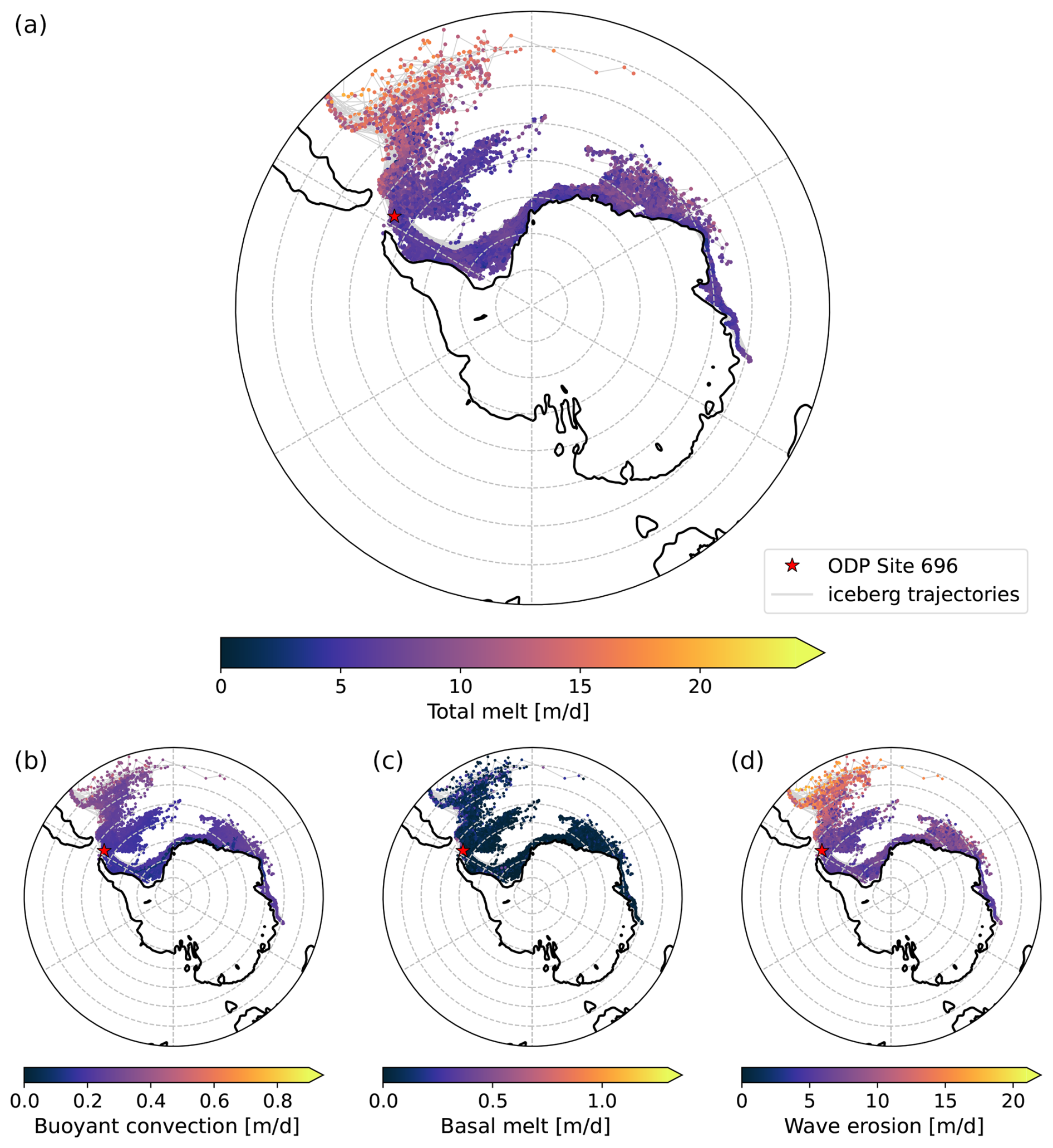
Figure 7 Spatial distribution of the total (a) and individual iceberg melt terms (b, c, d; see Fig. 2) along iceberg trajectories for icebergs of size class C4 during a 5-year-long forward simulation. Note that the marker of ODP Site 696 is roughly half (equal to) the size of the SOM in panel (a) (panels b, c, d).

Basal melt still lies within the range of melt rates observed in the present day (Cenedese and Straneo, 2023), although we should note that the magnitude of this term might be underestimated for large icebergs (FitzMaurice and Stern, 2018). The other melt terms – especially wave erosion – are much larger than at present. As buoyant convection is strongly temperature-dependent, the higher Eocene temperatures explain the increased melt rate. Similarly, Kubat et al. (2007) suggested that wave erosion can increase with up to 1 m d⁻¹ per degree temperature. With late Eocene surface temperatures at the Antarctic coast around 10 °C (Fig. 1c), the high magnitude of this term does not seem unreasonable and, taking into account that the modelled temperatures are probably overestimated due to the lack of ice in the model, might even be somewhat lower.

However, as stated before, monthly wind stress data were used to calculate wave erosion. Based on a comparison in the present day (Sect. S3.1.4), this could underestimate wave erosion rates by 4 % to 46 % (average 31 %). Hence, the late Eocene wave erosion rates might be even larger, and, more importantly, the lifetime of icebergs might be overestimated, which could especially affect the likelihood of smaller and/or more distantly released icebergs reaching ODP Site 696. This could alter the potential provenance regions to ODP Site 696, especially for the more distal regions. Moreover, a change in melt rates might lead to a difference in trajectories. For a modern comparison, this difference appeared to be minor (Fig. S3.5, Sect. S3.1.4). Nevertheless, as this simulation occurred in the much colder present-day setting, which is expected to have lower melt rates, the impact might only become visible after a longer simulation period.

Finally, it should be noted that, while the magnitude of melt rates gives a good sense of the impact of environmental conditions on the iceberg, their magnitude is independent of the iceberg's size. Hence, the ratio between the melt terms in units of megatons per day (Mt d⁻¹) can show a different contribution of each melt term. Notably, wave erosion only works on two of the iceberg sides (Fig. 2c). For large iceberg masses, the vertical scale of the iceberg (thickness) is usually much smaller compared to the horizontal scale. Therefore, even a small basal melt rate might lead to a large loss of iceberg mass when the horizontal iceberg area is large.

In short, whilst the late Eocene iceberg melt rates are significantly higher than those found nowadays, their magnitude seems fitting for the warm Eocene climate and still allowed larger icebergs to reach ODP Site 696. However, both basal melt and especially wave erosion might be underestimated for (large) icebergs, hence potentially reducing the iceberg lifetimes, which might impact the probable IRD provenances. On the other hand, the lack of ice in the forcing model might lead to an overestimation of temperatures, hence increasing the iceberg's lifetime.

4.5 Model sensitivity

Finally, we analyse the sensitivity of the results to several variables.

4.5.1 Doubled target radius

Allowing icebergs passing within a larger radius of ODP Site 696 to be included leads to an additional region, the Ellsworth Mountains, able to release icebergs to the site. The more proximal location of this region also slightly reduces the minimum iceberg mass to 100 Mt for size class C1, 150 Mt for C2, and 1750 Mt for C3. The effect on iceberg thickness differs per size class, showing a size increase to 21 m for C1 and a decrease to 26 and 205 m for C2 and C3, respectively. Overall, the iceberg size appears not to be reduced significantly, and the main effect lies with a change in the possible source locations and hence the provenance of IRD. In addition, similar effects might be expected for the other initial size classes (C3, C5).

4.5.2 Surface-only flow

From the simulation using only surface fields, it appears that all regions might contribute to the IRD at ODP Site 696 to at least some degree. In addition, this seems to lead to slightly smaller most probable minimum iceberg masses and thicknesses compared to the depth-integrated simulation. Apparently, although the higher temperatures at the surface increase the iceberg melt rates – and as such would lead to faster size changes – the increase in iceberg velocity leads to only minor differences in iceberg size spatially. However, the difference in iceberg trajectories is significant and, as grounding is not included, non-physical.

5 Conclusions

This study aimed to simulate late Eocene iceberg trajectories in the southern Weddell Sea region to test whether these match the proxy evidence by Carter et al. (2017) for iceberg-delivered debris found at ODP Site 696 at the SOM. As stated in the Introduction, we determined that, if the IRD is indeed derived from Antarctica, our simulations must demonstrate (1) that icebergs derived from the southern Weddell Sea region can reach ODP Site 696 before having melted away, (2) which regions are most likely to have released icebergs, and (3) what the minimum size of the icebergs leaving Antarctica must be in order to survive the flow path from Antarctica to ODP Site 696.

Our experiments have shown that icebergs released at the Antarctic coast can indeed reach ODP Site 696 before melting away. Specifically, icebergs derived from offshore the Filchner Ice Shelf and Dronning Maud Land are the most likely source regions for IRD found at ODP Site 696 based on possible trajectories and geological composition. The minimum size of icebergs leaving the coast from these regions must have been on the order of at least 100 Mt or several tens of metres in thickness to survive the flow path from Antarctica to ODP Site 696 at the SOM. Although this mass is at the larger end of the present-day range of common iceberg masses around Antarctica, the minimum estimates are not unfeasible. Hence, the present study confirms previous findings suggesting glaciation and iceberg calving were possible in the late Eocene. Specifically, as the target radius used here is quite conservative, using a larger radius would increase the likelihood of icebergs reaching the site, add additional potential source regions, and widen the possible range of iceberg sizes.

A limitation of this study is the use of monthly instead of daily wind fields. A simulation in the present day showed this underestimates wave erosion and hence overestimates iceberg lifetime. Further research might explore alternative ways of accounting for this deviation during the simulations. In addition, while expansion of the model by inclusion of other iceberg forcings would particularly improve the trajectories of smaller icebergs, adding a parameterisation of iceberg fracturing will improve the trajectories of icebergs in the larger size classes. Finally, as grounding was shown to have a significant impact on the iceberg trajectories, simulating different iceberg size classes with various thicknesses could reveal different potential regions of provenance.

Appendix A: Number of icebergs reaching ODP Site 696

Table A1 Total number and percentage of forward iceberg releases reaching ODP Site 696 within a distance of 1 grid cell (∼ 11 km) for each iceberg size class (C1–C5) and the sensitivity simulations for size class C4 with inclusion of icebergs passing ODP Site 696 at twice the distance of a grid cell (∼ 22 km; “doubled target radius”) or when using only surface fields (“surface only”).

Appendix B: Data points per region

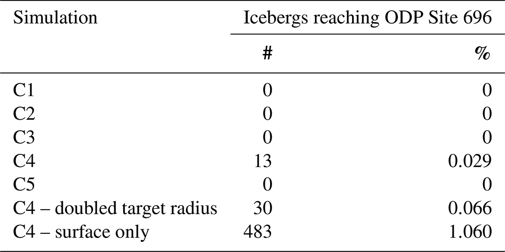
Table B1 Number of data points in each coastal region (Fig. 1; where PL is Palmer Land, EM is the Ellsworth Mountains, FIS is the Filchner Ice Shelf, CL is Coats Land, and DML is Dronning Maud Land (W: west; E: east)) and in total for each backward simulation (iceberg size classes C1–C3 and sensitivity simulation of size class C1 using only surface fields). The number of data points reflects the total number of times any iceberg is located within the indicated coastal region during the 5-year simulation period (e.g. for class C1 in region DMLE, the presence of an iceberg has been recorded eight times. This could have been the same iceberg during 8 time steps, eight different icebergs present at 1 time step each, or a combination of those).

Appendix C: Minimum iceberg size per region

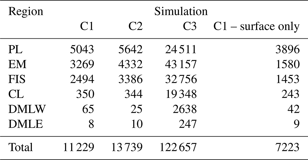
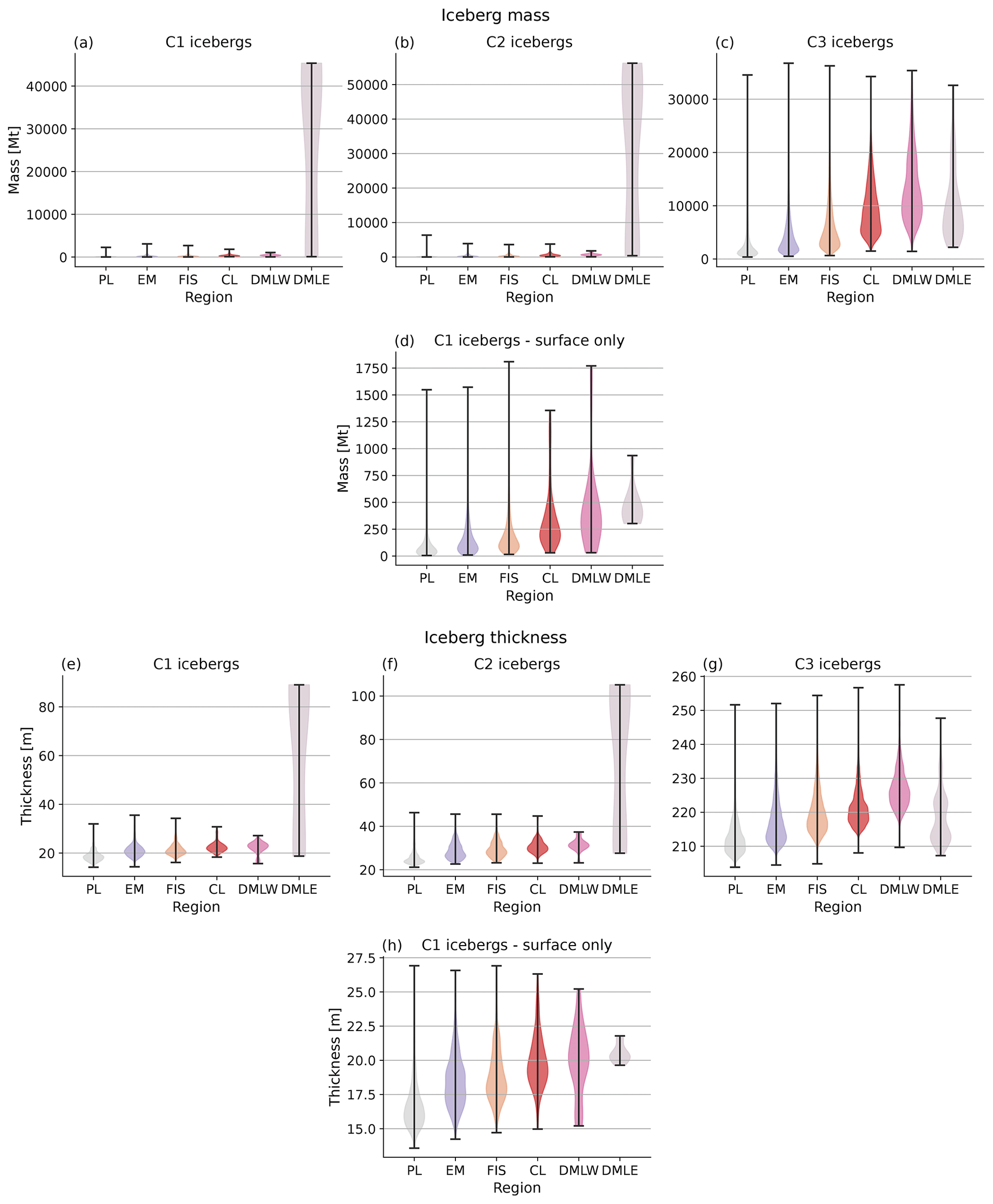
Figure C1 Visualisation (violin plot) of the complete mass and thickness distributions obtained with backward simulations for (a–d) the minimum iceberg mass and (e–h) the minimum iceberg thickness in each coastal region (Fig. 1), where PL is Palmer Land, EM is the Ellsworth Mountains, FIS is the Filchner Ice Shelf, CL is Coats Land, and DML is Dronning Maud Land (W: west; E: east). (a–c, e–g) Results of the main backward simulations run for size classes C1, C2, and C3. (d, h) Results of the sensitivity simulation run for size class C1 when using only surface fields. See Fig. 6 for more details in the lower range.

Appendix D: Modern model fields

Figure D1 Regional time-mean (1 year) ocean properties from the MOi hydrodynamics model (Gasparin et al., 2018) for (a) the velocity in the surface layer, (b) the temperature at the surface (∼ 0–200 m), and (c) ocean streamlines.

Appendix E: Eocene streamlines

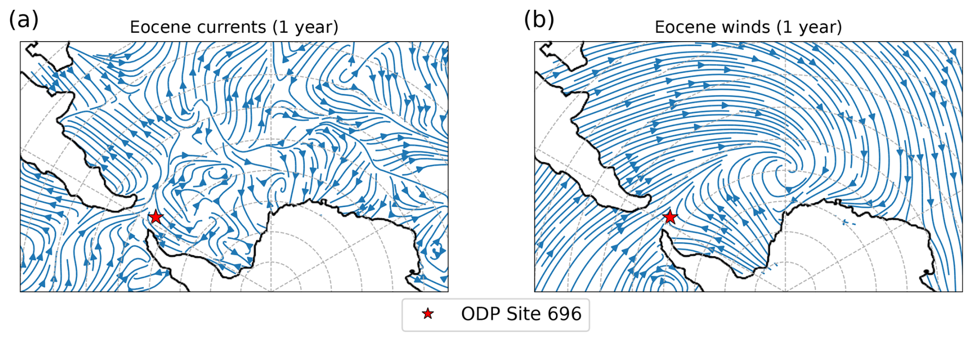
Figure E1 Streamlines of Eocene (a) ocean currents and (b) winds around Antarctica.

Appendix F: Iceberg trajectories at the SOM

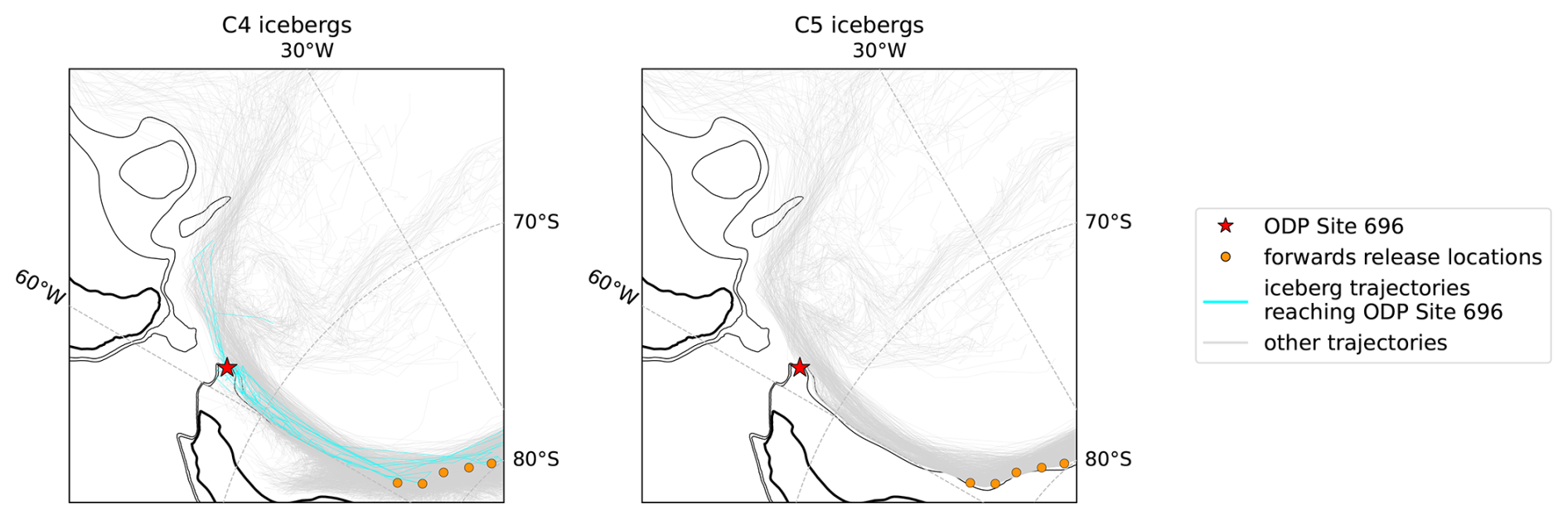
Figure F1 Forward trajectories of depth-integrated simulations (iceberg size class C4 and C5) around ODP Site 696 and the SOM that can (blue) or cannot (grey) reach ODP Site 696 at some point along their trajectory. In addition to the coastlines (bold), the 250 and 500 m bathymetry lines are shown. Note that the marker of ODP Site 696 is roughly one-sixth of the size of the SOM.

Appendix G: Iceberg lifetime

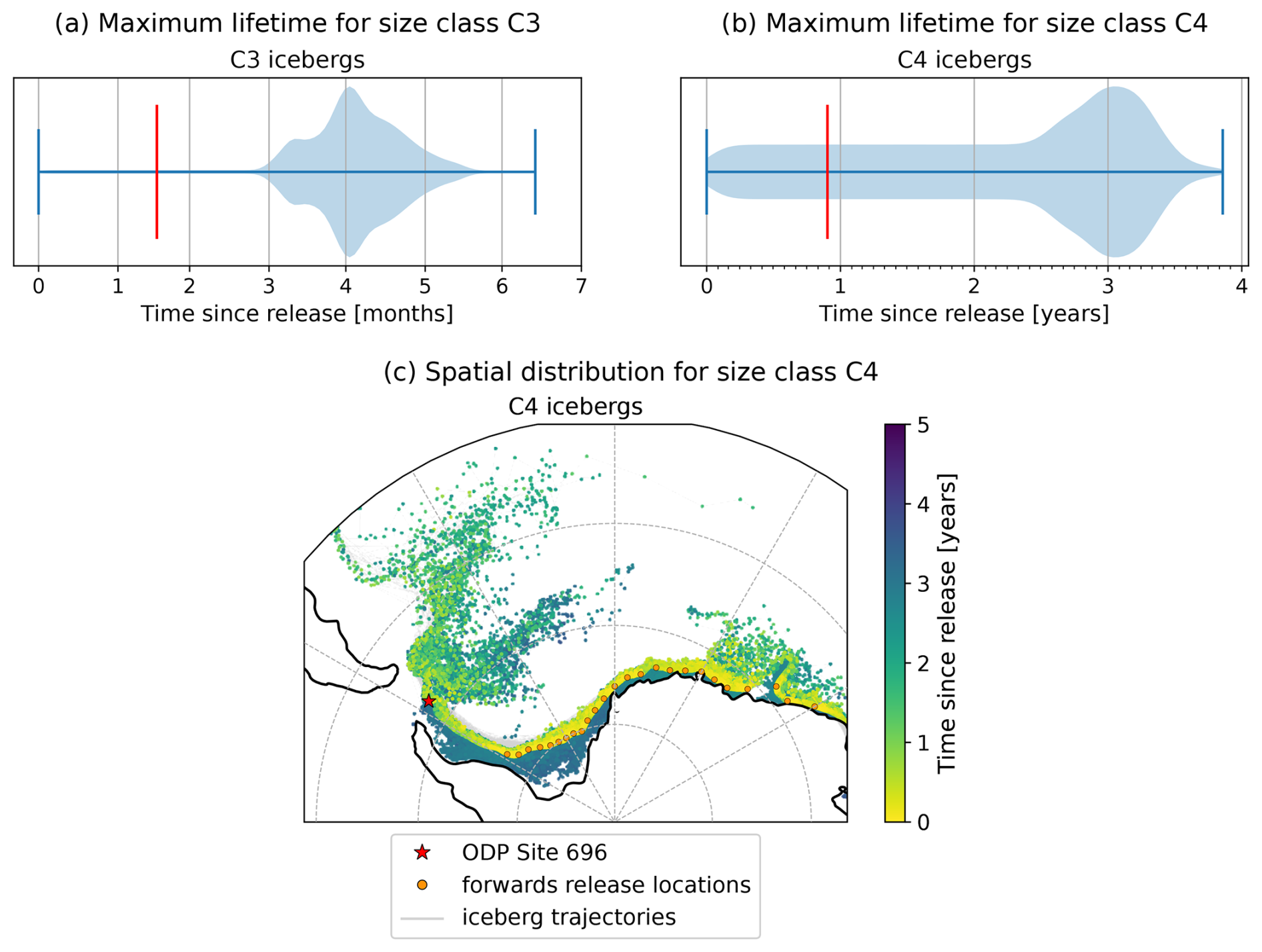
Figure G1 Distributions of iceberg lifetime through time (C3, C4) and space (C4) for forward simulations. The red lines in panels (a) and (b) indicate the mean iceberg half-lives. Note that the marker of ODP Site 696 is roughly one-quarter of the size of the SOM.