Modelling the impact of palaeogeographical changes on weathering and CO₂ during the Cretaceous–Eocene period

The feedback between atmospheric CO₂ concentrations and silicate weathering is one of the key controls on the long-term climate of the Earth. The potential silicate weathering flux (as a function of conditions such as temperature, runoff, and lithology), or “weatherability”, is strongly affected by continental configuration; thus the position of continental landmasses can have substantial impacts on CO₂ drawdown rates. Here, we investigate the potential impact of palaeogeographical changes on steady-state CO₂ concentrations during the Cretaceous–Eocene period (145–34 Ma) using a coupled global climate and biogeochemical model, GEOCLIM, with higher-resolution climate inputs from the HadCM3L general circulation model (GCM).

We find that palaeogeographical changes strongly impact CO₂ concentrations by determining the area of landmasses in humid zones and affecting the transport of moisture, that runoff is a strong control on weatherability, and that changes in weatherability could explain long-term trends in CO₂ concentrations. As Pangaea broke up, evaporation from the ocean increased and improved moisture transport to the continental interiors, increasing runoff rates and weathering fluxes, resulting in lower steady-state CO₂ concentrations. Into the Cenozoic, however, global weatherability appears to switch regimes. In the Cenozoic, weatherability appears to be determined by increases in tropical land area, allowing greater weathering in the tropics.

Our modelled CO₂ concentrations show some strong similarities with estimates derived from proxy sources. Crucially, we find that even relatively localised changes in weatherability can have global impacts, highlighting the importance of so-called weathering “hotspots” for global climate. Our work also highlights the importance of a relatively high-resolution and complexity-forcing GCM in order to capture these hotspots.

1 Introduction

One of the key controls on the long-term climate of the Earth is the concentration of atmospheric CO₂. Throughout Earth's history, concentrations of CO₂ in the atmosphere have changed substantially, for example, from several thousand parts per million (ppm) in the early Phanerozoic to under 200 ppm during the Last Glacial Maximum (e.g. Royer, 2006; Bouttes et al., 2011; Foster et al., 2017). Atmospheric CO₂ concentrations are ultimately determined by the balance of CO₂ emitted from volcanic sources (volcanic degassing), and the drawdown of CO₂ is determined by the chemical weathering of silicate rocks (Berner et al., 1983). This “simple” balance is complicated by the complexity of chemical weathering processes, especially in the geological past. It should be noted that the burial of organic matter is also significant for atmospheric CO₂ concentrations (e.g. Berner, 1990; Hilton and West, 2020). The impact and extent of this process can be difficult to quantify in the geological past and is not assessed as part of this study.

Chemical weathering rates of silicate minerals are sensitive to climate variables, such as temperature and precipitation, in addition to intrinsic factors (i.e. factors inherent to the rocks themselves, such as lithology) (Strakhov, 1967; Walker et al., 1981; Berner et al., 1983; White and Blum, 1995; Oliva et al., 2003; West et al., 2005). While there is evidence from individual sites that weathering is accelerated under warm, humid conditions (e.g. White and Blum, 1995), it is unclear whether such a trend can be applied at the global scale. Evidence from field and modelling studies of weathering profiles suggests a stronger precipitation- or runoff-based control on weathering rates than temperature (e.g. Oliva et al., 2003; Maher, 2010; Hayes et al., 2020), while global models (e.g. GEOCARB and derivatives) have often invoked temperature as a stronger control (Berner et al., 1983; Berner and Kothavala, 2001). Other global models, including GEOCLIM, have suggested that runoff may be a more significant control on weathering rates and thus long-term climate (Goddéris et al., 2014). The geographical distribution of lithology may play a role (e.g. Donnadieu et al., 2004), but palaeolithologies are difficult to constrain.

General circulation models (GCMs) have been used extensively to model climates on multi-million-year timescales (e.g. Lunt et al., 2021). These models have been evaluated using records from proxies such as stable isotope ratios, TEX86, Mg $/$ Ca ratios, and alkenones (e.g. Hutchinson et al., 2021). Although GCM simulations do not always produce results that agree with proxy data (e.g. Huber and Caballero, 2011; Keating-Bitonti et al., 2011; Lunt et al., 2012; Jagniecki et al., 2015), they have greatly expanded the spatial knowledge of past climates, whereas proxy data have been gathered from a comparatively limited number of sites (e.g. Huber and Caballero, 2011). Furthermore, proxy data often produce conflicting reconstructions, such as differing atmospheric CO₂ levels (e.g. Jagniecki et al., 2015) or significantly different temperature and precipitation reconstructions (e.g. Keating-Bitonti et al., 2011). GCMs can be used to reconstruct global climates based on different proxy records and compare the results (e.g. Huber and Caballero, 2011; Lunt et al., 2012, 2016). Thus, GCMs have become a powerful tool in reconstructing palaeoclimates.

The large quantities of GCM-derived climate outputs have been incorporated into global geochemical models over the last 10–15 years (e.g. Berner and Kothavala, 2001; Donnadieu et al., 2004), enabling some of those models to provide spatially varying estimates of global weathering rates under different climate and palaeogeographic configurations. However, as noted above, these climate reconstructions can vary significantly depending on the model configuration and the boundary conditions used.

Controls on Mesozoic–Cenozoic climate

Over multi-million-year timescales, climates during the Mesozoic and Cenozoic were affected by a gradual increase in solar forcing and, in general, a gradual decrease in CO₂ forcing (Foster et al., 2017, Fig. 1). A number of theories have been advanced to explain changes in atmospheric CO₂, and thus climate, over multi-million-year timescales. The gradual breakup of Pangaea and the associated rifting likely resulted in increased volcanic degassing fluxes (Tajika, 1998; Lee and Lackey, 2015; Lee et al., 2015). The Late Cretaceous and the Cenozoic saw a period of mountain building associated with the latter stages of the breakup of Pangaea. The Laramide orogeny began approximately 70 Ma (Humphreys et al., 2003), and the development of the northern Andes and the Himalayas occurred during the early Cenozoic (Schellart, 2008). The development of new mountain ranges, particularly the Himalayas, has been implicated in the reduction of CO₂ concentrations during the Cenozoic by increasing silicate weathering rates and thus increasing CO₂ drawdown (Raymo and Ruddiman, 1992). Changes in weathering fluxes have been linked to a number of climate shifts in the Earth's past, such as the global cooling which occurred during the Carboniferous (e.g. Goddéris et al., 2014, 2017).

Changes in palaeogeography can have substantial effects (Lunt et al., 2016). For example, the presence of mountain ranges may affect monsoon circulation and thus precipitation, or the presence of large continental interiors isolated from moisture can lead to large arid deserts. As such, the potential silicate weathering flux, or “weatherability”, of the continents is likely to represent a key climate forcing during the late Mesozoic–early Cenozoic and forms the focus of this study.

At steady state, silicate weathering fluxes are equal to emissions from volcanic degassing (e.g. Walker et al., 1981; Berner et al., 1983; Goddéris et al., 2014). However, a distinction should be drawn between weathering (here, the chemical breakdown of silicate rocks by water and carbonic acid) and “weatherability”. Weatherability corresponds to the susceptibility of the land surfaces to be weathered, under a given climate (temperature and runoff) (Kump and Arthur, 1997). Weatherability can be affected by the presence of land plants impacting relief and erosion rates (through the exposure of fresh material to weathering), by changes in the lithology, or by the palaeogeographic configuration (Dessert et al., 2003; Oliva et al., 2003; West et al., 2005; Maher, 2010; West, 2012; Bazilevskaya et al., 2013; Bufe et al., 2024). The role of land plants is difficult to constrain, and studies have produced contrasting results (e.g. Porada et al., 2016; Goddéris et al., 2017), so vegetation is often excluded or held constant within simulations of weathering.

Global palaeolithologies are poorly constrained and become even less so further back into the geological record. Similarly, factors such as topography and uplift rates, which affect erosion rates (e.g. Riebe et al., 2004; West et al., 2005; Gabet and Mudd, 2009), are also poorly constrained into geological time. In contrast, broad-scale climate parameters, such as temperature and precipitation patterns, are comparatively well constrained through proxy data and GCM studies. Climate states are in turn strongly controlled by the positioning of the continents, which can affect oceanic and atmospheric circulation patterns (e.g. Gyllenhaal et al., 1991; Von der Heydt and Dijkstra, 2006). The positioning of the continents also affects weatherability by determining the land area in intense weathering environments, such as the tropics (e.g. Goddéris et al., 2014).

In this study, we focus on the impact of the palaeogeographic setting on the weatherability, assuming that all the other factors remain constant over the simulated period (this is certainly not the case, but our objective is to quantify exclusively the role of palaeogeography).

For an idealised case where degassing is constant (Walker et al., 1981), the global weathering flux will equilibrate the volcanic degassing of CO₂, and the global CO₂ consumption by silicate rock weathering will stay constant. However, the evolving continental configuration modulates weatherability, allowing CO₂ to fluctuate (Goddéris et al., 2014).

In contrast to palaeo-degassing rates, palaeogeographies (within the last 150 million years) are relatively well constrained. Thus, there is scope to investigate the impact of changing weatherability on long-term CO₂ concentrations. Early studies using zero-dimensional global models, such as GEOCARB, used estimations of global mean annual temperature (MAT) and runoff values, but no geographical constraints, to estimate global weathering fluxes and steady-state CO₂ concentrations in geological time (Berner, 1991). Further studies refined the GEOCARB approach by including palaeogeographical reconstructions, both conceptual (e.g. “ringworld” configurations) and realistic, which demonstrated that continental configurations had significant impact on steady-state CO₂ concentrations (e.g. Barron et al., 1989) and that palaeogeography and climate interact to determine steady-state CO₂ concentrations (Otto-Bliesner, 1995). Further model developments provided spatial patterns in climate-forcing data, demonstrating that regional changes in weatherability can have global climate impacts (Donnadieu et al., 2004). More recently, such models have shown that the positioning of the continents also affects weatherability by determining the land area in intense weathering environments, such as the tropics (e.g. Goddéris et al., 2014).

The impact of changing weatherability as a result of changes in palaeogeography during the Phanerozoic was previously investigated by Goddéris et al. (2014) using GEOCLIM with climate inputs from the GCM, FOAM, which found that the formation of supercontinents resulted in a continental configuration favourable for high atmospheric CO₂ concentrations (10–25 × PAL), as the converged continental configuration resulted in arid continental interiors and reduced weatherability. Conversely, dispersed continental configurations were more favourable to lower atmospheric CO₂ concentrations (1–8 × PAL) by favouring higher continental runoff and weatherability. Furthermore, Goddéris et al. (2014) found that continents or even smaller landmasses crossing warm humid climate belts can result in significant drawdown of atmospheric CO₂. For example, during the Late Triassic, the gradual northward drift of Pangaea brought larger areas of landmass into more humid zones. In response, CO₂ concentrations fell sharply over ∼ 20 Myr from 19 × PAL to 3 × PAL (Goddéris et al., 2014).

Goddéris et al. (2014) had a relatively low temporal resolution of 22 simulations over the last ∼ 520 Myr (approximately 1 simulation per 20–30 Myr) to produce a simulated CO₂ record and, from that, glean insights on the effects of changing weatherability (through palaeogeographical changes) on long-term CO₂ concentrations and thus global climate. In contrast, this study will use 19 simulations over the Cretaceous–Eocene period (145–36 Ma) in addition to better-constrained and higher-resolution (factor of 3.65 increase) palaeogeography and climate inputs to produce our own simulated CO₂ record, assuming a constant degassing rate. The higher temporal resolution will allow the investigation of the impacts of higher-temporal-resolution changes (∼ 5 Myr) in palaeogeography on long-term CO₂ and weatherability, while the higher spatial resolution will better constrain regional variability in weatherability relative to Goddéris et al. (2014). The use of climate inputs produced by the more complex HadCM3L in this study (relative to the FOAM inputs used by Goddéris et al., 2014) also represents an improvement. These model-based improvements should provide a more accurate picture of how global climate responds to changes in weatherability and should better constrain the role of chemical weathering feedbacks on global climate through geological time.

2 Methodology

This study will investigate the impact of varying palaeogeography from the Early Cretaceous to the late Eocene on weatherability, using a coupled global climate and geochemical model, GEOCLIM, with climatic reconstructions derived from HadCM3L.

2.1 GEOCLIM

GEOCLIM is a coupled global climate and biogeochemical model initially developed in the early 2000s and has been used to investigate interactions between climate and geochemistry in deep time settings on geological timescales (Donnadieu et al., 2004). GEOCLIM uses temperature and runoff inputs from climate models at specified CO₂ concentrations (e.g. 280, 560 ppm) and models the climate conditions through interpolation between as atmospheric CO₂ concentrations evolve within GEOCLIM simulations. Should CO₂ concentrations in GEOCLIM fall outside of the specified range, it will be unable to update climate conditions and thus will use climate conditions associated with the nearest available CO₂ concentration. GEOCLIM initially used CLIMBER inputs in early studies (Donnadieu et al., 2004), but more recent studies have used FOAM inputs (Lefebvre et al., 2013; Goddéris et al., 2014, 2017).

COMBINE, a model within GEOCLIM, handles biogeochemical processes for both land and ocean environments. Oceans are divided into nine “boxes”: two high-latitude oceans (> 60° N/S) (each separated into a photic layer and a deep-ocean layer); a low- to mid-latitude ocean (60° S–60° N) divided into photic, thermocline, and deep-ocean layers; and an epicontinental sea also divided into photic and deep layers. A final 10th box represents the atmosphere. A range of biogeochemical processes are modelled within the ocean layers. As this study focuses on terrestrial processes, we will omit a detailed description of the ocean processes, but full descriptions can be found in Goddéris and Joachimski (2004) and Donnadieu et al. (2006).

Chemical weathering in GEOCLIM occurs in terrestrial grid cells, and the total sum value of silicate weathering from each terrestrial grid cell, along with a prescribed volcanic degassing value, is used to calculate changes in atmospheric CO₂ at each time step. Ocean carbon and alkalinity are kept balanced at steady state. Chemical weathering calculations for silicate rocks are based on equations from Oliva et al. (2003) and Dessert et al. (2003).

$$\begin{array}{}\text{(1)}& F_{\mathrm{sil}}\left(t\right)=k_{\mathrm{sil}}\times \left({\mathit{\alpha }}_j\left(t\right)\times {\mathit{\rho }}_j\left(t\right)\times A{e}^{-E_{\mathrm{a}}/RT}\right)\end{array}$$

Equation (1) calculates the granitic weathering flux in moles of C per year at a time step (t) in a given grid cell, F_sil(t); k_sil is the silicate weathering constant; α_j(t) is the area of a grid cell (10⁶ km²); and ρ_j(t) is the runoff value of that grid cell (cm yr⁻¹). The final term (dimensionless) is an Arrhenius equation for granite weathering, representing the granitic dependence on dissolution based on air temperature (T) and the universal gas constant (R), which uses the activation energy for granite (E_a) defined by Oliva et al. (2003) and the air temperature in a given grid cell, T_j.

$$\begin{array}{}\text{(2)}& F_{\mathrm{bas}}\left(t\right)=k_{\mathrm{bas}}\times \left({\mathit{\alpha }}_j\left(t\right)\times {\mathit{\rho }}_j\left(t\right)\times A{e}^{-E_{\mathrm{a}}/RT}\right)\end{array}$$

A similar calculation exists for basalt (Eq. 2), based on values in Dessert et al. (2003), and for carbonate rocks. Both calculations were derived from and calibrated on weathering reaction processes within granite and basaltic watersheds, described in detail in Oliva et al. (2003) and Dessert et al. (2003), respectively. We omit the carbonate equation here, as this study focuses on variations in CO₂ drawdown via changes in silicate weathering fluxes. GEOCLIM assumes that each grid cell has an equal area of granitic, basaltic, and carbonate rocks. While this is obviously a significant simplification of the real-world geology of the time, palaeolithologies are poorly constrained. In the absence of reliable global palaeolithologies from the studied time period, we assume an even distribution of lithologies for simplicity and consistency with Goddéris et al. (2014). A newer version of GEOCLIM, recently developed, includes an erosion dependency on chemical weathering rates based on equations in Gabet and Mudd (2009) (Maffre et al., 2021). As a key part of this study relates to comparing our new simulations to previous results with GEOCLIM (Goddéris et al., 2014), this version of the model was not used in this study for reasons of consistency. The most recent version of GEOCLIM, GEOCLIM7, is fully detailed in Maffre et al. (2024).

2.2 HadCM3L

HadCM3L is part of the HadCM3 “family” of coupled GCMs originally developed by the UK Met Office (Gordon et al., 2000; Valdes et al., 2017). The HadCM3 family of models has been in use for over 15 years, with various modifications to the configuration of the original model, HadCM3, being made in that time. HadCM3L is a version of HadCM3 using a “low-resolution” ocean, where ocean and atmosphere share the same 96 × 73 (3.75° × 2.5°) resolution (Valdes et al., 2017). Although described as “low-resolution”, 96 × 73 is nonetheless 3.65 times higher resolution than FOAM. However, like FOAM, HadCM3L is used for long-term simulations where higher-resolution models would be too time-intensive to be practical. To that end, HadCM3L has been used extensively in pre-Quaternary climate studies, where long-term climate simulations are required (e.g. Lunt et al., 2010, 2011, 2012; Valdes et al., 2017). This study uses climate inputs from 19 HadCM3L simulations of the Cretaceous–Eocene period at intervals of 3–13 Ma, the same simulations used by Farnsworth et al. (2019). These simulations were run with CO₂ concentrations at 560 and 1120 ppm, which are considered to be a reasonable representation of potential CO₂ concentrations during the Cretaceous–Eocene, which are subject to considerable uncertainty (Lunt et al., 2016). To match the range of climate conditions at the 11 concentrations used for the FOAM climate inputs (160–1400 ppm) in Goddéris et al. (2014), the HadCM3L climate inputs were extrapolated from the two CO₂ concentrations (560–1120 ppm) to the same 11 concentrations (Appendix A). This process was devised and evaluated using a sensitivity study in Hayes (2019) and was found to be robust, although this is largely irrelevant, as the modelled CO₂ concentrations produced remained very close to or within the 560–1120 ppm range. The simulations in Farnsworth et al. (2019) (used for this study) slightly differ from those in Lunt et al. (2016) in that they have a spinup time of 10 422 years, as opposed to 1422 years in Lunt et al. (2016). The extended spinup time was to enable the simulations to more closely approach an equilibrium state and to make use of the fully dynamic mode within the coupled vegetation model. Runoff calculations are affected by the vegetation model, with both canopy interactions and soil infiltration considered within HadCM3L. A full description of the runoff parameterisation can be found in Gregory et al. (1994). Estimating uncertainties in modelled runoff is challenging, but the higher resolution of HadCM3L relative to FOAM is likely to provide a better parameterisation of features significant to runoff, such as relief, even when accounting for uncertainties in reconstructing palaeo-relief.

The palaeogeographic reconstructions used in this study were developed by Getech for Lunt et al. (2016). The reconstructions were produced using methods developed by Markwick and Valdes (2004) and include data from well-constrained geological databases, such as The Paleogeographic Atlas Project. These palaeogeographies were originally constructed at 0.5° × 0.5° resolution – topographies, bathymetries, and land–sea masks were generated from these high-resolution palaeogeographies at 3.75° × 2.5° resolution for HadCM3L (Lunt et al., 2016). Additionally, HadCM3L is coupled to the Top-down Representation of Interactive Foliage and Flora Including Dynamics (TRIFFID), which is a dynamic global vegetation model (Cox et al., 2002). The two modules are coupled via the MOSES 2.1 land surface scheme (Cox et al., 1999). The TRIFFID model calculates the fraction of five plant functional types (broadleaf trees, needleleaf trees, C₃ grasses, C₄ grasses, and shrubs) in each grid cell. Although these are modern plant types, studies have suggested that models such as TRIFFID can nonetheless perform acceptably in providing vegetation feedback signals back to at least 250 million years (Donnadieu et al., 2009; Zhou et al., 2012). Estimating uncertainties introduced by the vegetation model is challenging; however, Donnadieu et al. (2009) indicate that vegetation models adequately reproduce the spatial distributions of major biogeographical areas, such as desert, temperate, and polar regions.

2.3 GEOCLIM configuration

The degassing rate for the palaeogeography simulations was set to a constant value of 1 × 10¹³ mol C yr⁻¹, similar to previous GEOCLIM studies (Lefebvre et al., 2013). A value of 1 × 10¹³ mol C yr⁻¹ is within the range of estimates (∼ 1.2–2 times modern) for degassing rates during the Cretaceous–Eocene period (Van Der Meer et al., 2014). These simulations were also run using variable degassing rates ranging from a low value of 7.82 × 10¹² mol C yr⁻¹ in the latest Eocene to a high of 1.23 × 10¹³ mol C yr⁻¹ in the Early Cretaceous (Appendix Fig. A1). This range is based on values calculated by Van Der Meer et al. (2014) using reconstructed subduction zone arc lengths.

We conducted two sets of experiments. We ran one simulation per time slice, fixing the initial atmospheric CO₂ to 2.85 times the pre-industrial value of 280 ppm (∼ 800 ppm). This CO₂ concentration is intermediate between the 560 and 1120 ppm reconstructions. The first set of experiments allows us to isolate the effect of the palaeogeography on the weatherability of the continental surfaces, all other factors being fixed. The second set of experiments was conducted by allowing GEOCLIM to run until atmospheric CO₂ reached steady state to provide an estimate of atmospheric CO₂ under the aforementioned palaeogeographical and climate conditions. Atmospheric CO₂ will adapt in response to weathering until global silicate weathering fluxes compensate for solid Earth degassing.

3 Results

Our simulations for the 19 time slices produced a simulated CO₂ record from 145–36 Ma. Throughout the Results and Discussion, patterns within the record will be compared with changes in global weathering fluxes and climate variables to investigate if, and how, changes in weatherability have affected the CO₂ record. To begin, we discuss the role of degassing and silicate weathering fluxes in driving these variations.

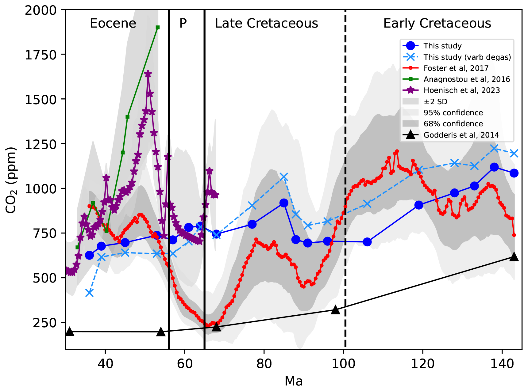
Figure 1 Steady-state CO₂ as modelled by GEOCLIM plotted against three CO₂ proxy records from the literature and simulated record from Goddéris et al. (2014). The GEOCLIM output displays some agreement with the record from Foster et al. (2017), particularly during the Early Cretaceous (where CO₂ concentrations are comparably high), the Late Cretaceous, and the late Eocene. The CO₂ record from The Cenozoic CO2 Proxy Integration Project Consortium et al. (2023) (referred to here as Hoenisch et al., 2023) is generally higher than the GEOCLIM output but shows a similar pattern in the Late Cretaceous and early Palaeocene. The record from Anagnostou et al. (2016) displays considerably higher CO₂ concentrations during the early Eocene than those in the GEOCLIM and Foster records but shows better agreement with both records towards the mid- and late Eocene. A second GEOCLIM output (dashed red line) displays the results of running GEOCLIM simulations using variable degassing rates calculated in Van Der Meer et al. (2014). Note: Palaeocene is abbreviated to P for brevity.

The GEOCLIM simulations of the 19 time slices resulted in a range of CO₂ concentrations, with the lowest value of ∼ 650 ppm at the end of the Eocene and the highest value of ∼ 1100 ppm during the Early Cretaceous (Fig. 1). Atmospheric CO₂ exceeds 1000 ppm during the Early Cretaceous but declines significantly to ∼ 700 ppm by the mid-Cretaceous. There is a brief increase in CO₂ around 85 Ma to ∼ 900 ppm, followed by a gradual decrease into the Cenozoic and through to the end of the Eocene. The simulations run with variable degassing rates produced a similar pattern, albeit with higher atmospheric CO₂ concentrations during the Early Cretaceous and lower concentrations in the late Eocene relative to the simulations using a constant degassing rate.

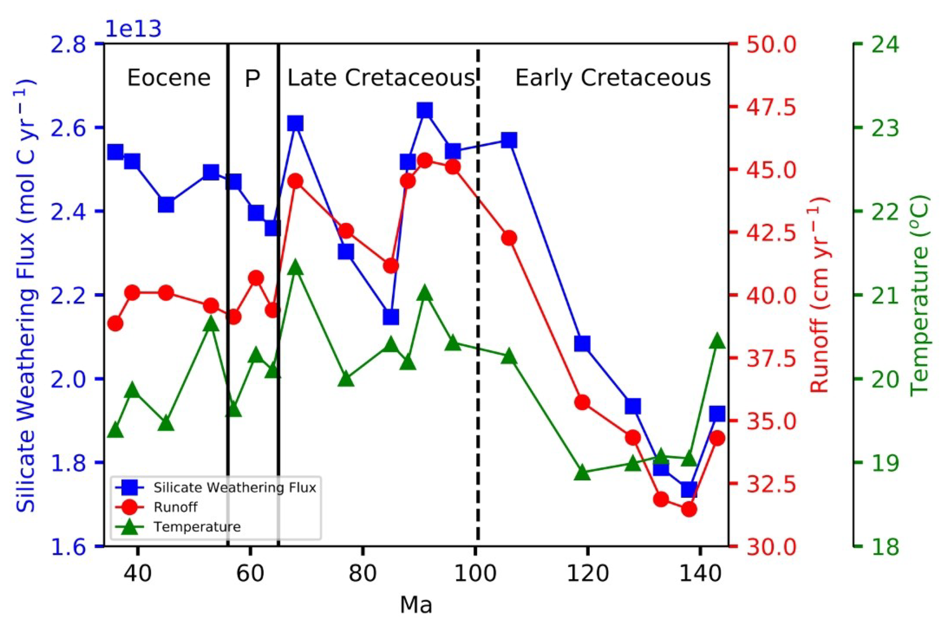
Figure 2 Modelled silicate weathering fluxes (blue squares) plotted against global mean annual runoff (red circles) and temperature (green triangles). Trends in silicate weathering fluxes are similar to those of global runoff but show less similarity to temperature. Note that Palaeocene has been abbreviated to P.

For the simulations performed with a fixed initial atmospheric CO₂ level at 2.85 times the pre-industrial value, the calculated global silicate weathering flux is inversely related to the atmospheric CO₂ concentrations produced by the simulations where atmospheric CO₂ was allowed to reach steady state (i.e. high initial silicate weathering fluxes result in lower steady-state CO₂ concentrations) (Fig. 2). The Early Cretaceous is marked by low silicate weathering fluxes, although fluxes increase significantly towards the mid-Cretaceous and peak at approximately 91 Ma. A brief, but sharp, decrease occurs until 85 Ma, followed by a similarly rapid recovery at the end of the Cretaceous to a similar level of weathering seen at 91 Ma. Another brief decrease occurs into the Palaeocene, followed by a gradual rise through the Eocene. Initial global mean temperature varies little throughout the Cretaceous–Eocene period, although a period of warming occurs in the mid- to Late Cretaceous, followed by gradual cooling into the Cenozoic. Farnsworth et al. (2019) noted in their simulations that temperature varied little with palaeogeography. Initial mean global runoff increases significantly into the mid-Cretaceous, followed by a brief decrease around 85 Ma and then an increase again towards the end of the Cretaceous. Runoff drops sharply at the start of the Palaeocene and remains mostly stable through the Eocene.

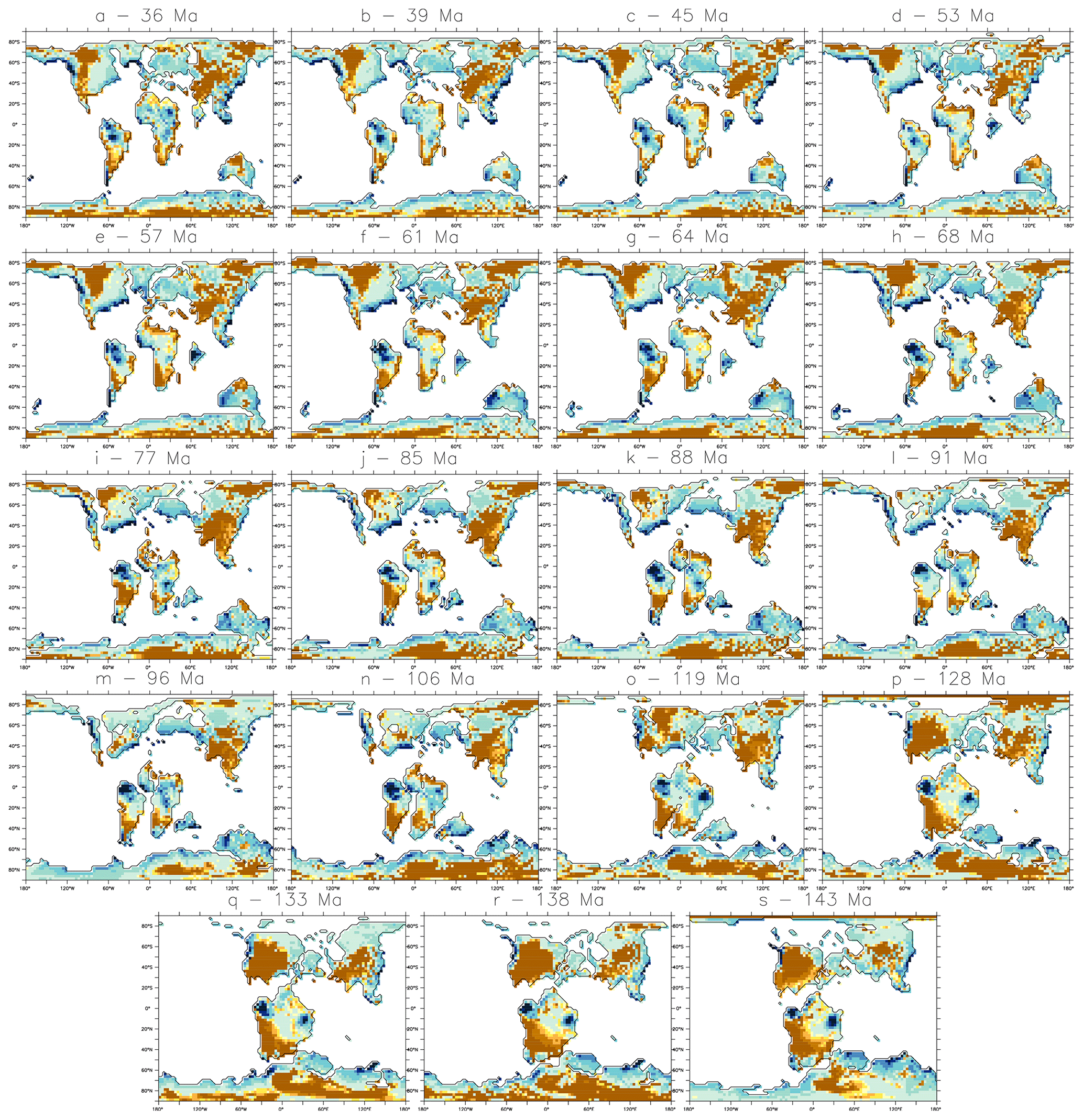
Figure 3 Regional mean annual runoff (cm yr⁻¹) maps from the earliest Cretaceous (s) to the latest Eocene (a). An arid climate prevails during the Early Cretaceous (s–o), particularly in the continental interior of North America. Runoff increases significantly from the mid-Cretaceous, with very high runoff rates present in Amazonia (m–k). High runoff totals are present in India during the latest Cretaceous and the Palaeocene as it crosses the Equator (h–e). The world becomes slightly more arid through the Eocene (d–a).​​​​​​​

In the fixed CO₂ simulations, the distribution of runoff changes significantly during the Cretaceous–Eocene period (Fig. 3). During the Early Cretaceous, large areas of North America, South America, Asia, and Antarctica have low or zero runoff, likely due to low moisture transport from the oceans given the converged continental configuration at this time. There are some areas of high runoff, such as the northern coast of Gondwana, along with parts of the western Amazon and eastern Africa. Into the mid- to Late Cretaceous, North America and Antarctica become much more humid, while Asia becomes more arid. The Amazon remains persistently humid, while the Atlantic coast of North America has high runoff, possibly due to increases in evaporation (and or tropical cyclones) associated with the expansion of the Atlantic. The west coast of North America has especially high runoff, with zonal means indicating that runoff here is greater than at the Equator, although runoff falls towards the Late Cretaceous. Into the Cenozoic, areas such as India and western Australia have a significant increase in runoff. India crosses the Equator at this time, so the increased runoff may be related to interactions with the ITCZ. Towards the end of the Eocene, areas such as North America and Asia become more arid, while runoff in the southern mid-latitudes increases slightly. Much of the world, however, becomes more arid, reflecting the global drop in runoff at the end of the Eocene, possibly linked to the general cooling trend and falling evaporation rates from the oceans from around 49 Ma into the Eocene–Oligocene boundary.

4 Discussion

Silicate weathering fluxes at 2.85 times the pre-industrial CO₂ show a strong relationship with mean global runoff rates and a strong inverse relationship with atmospheric CO₂ concentrations (Figs. 1–2 and Appendix Figs. A2–A3, r=0.88 and −0.96, respectively), indicating that changes in global runoff driving changes in silicate weathering fluxes are the primary control on steady-state CO₂ concentrations over the modelled period. However, there are some inconsistencies in these trends. Notably, global silicate weathering fluxes increase towards the late Eocene despite a fall in global runoff rates. To understand these inconsistencies in the global trend, we investigate the relationship between runoff rates and silicate weathering fluxes at the regional level.

4.1 Regional trends

During the Eocene, within the GEOCLIM simulations, both mean and total global runoff from the fixed CO₂ runs fall, yet silicate weathering fluxes rise, an inverse of the pattern seen during the Cretaceous, where runoff rates and weathering fluxes show identical patterns (Fig. 2). During the Early Cretaceous, silicate weathering fluxes are strongly controlled by non-tropical runoff (> 30° N/S), showing an almost identical pattern until the mid-Cretaceous (Fig. 4). This pattern weakens somewhat around 86 Ma but strengthens by the end of the Cretaceous. Into the Cenozoic, the pattern weakens again and silicate weathering fluxes become anti-phased to non-tropical runoff. In contrast, silicate weathering fluxes in the Eocene appear to be more strongly controlled by runoff rates in the tropics (Fig. 4). Similarly, tropical runoff changes in the Cretaceous do not appear to have a significant impact on silicate weathering fluxes, with the exception of a brief period during the Late Cretaceous (86 Ma). There is a noticeable weakening of the influence of non-tropical runoff on weathering fluxes from the Cretaceous to the Cenozoic, although, due to the small number of simulations in this period (n=6), confidence in this relationship is low.

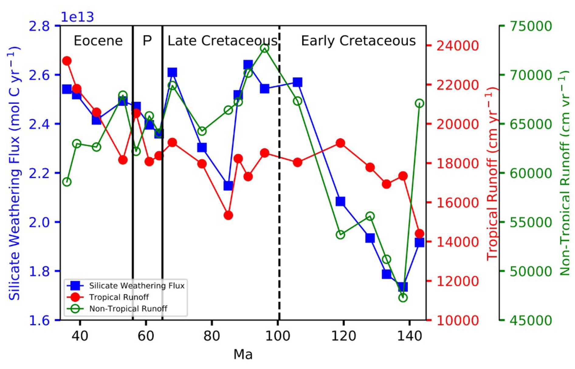
Figure 4 Modelled silicate weathering fluxes (blue squares) plotted against total tropical runoff (red circles) and total non-tropical runoff (green open circles). The tropics are defined here as all areas within 30° N/S. Changes in silicate weathering fluxes are driven broadly by non-tropical runoff during the Early Cretaceous and by tropical runoff during the Cenozoic. Note that Palaeocene has been abbreviated to P.

The shift from non-tropical- to tropical-runoff-controlled weathering appears to represent a regime change in the long-term climate pattern seen during the modelled period. Theoretically, a continental configuration with a greater land area in the low latitudes, where precipitation is generally highest, would favour lower global CO₂ concentrations by increasing silicate weathering rates (Gibbs and Kump, 1994; Otto-Bliesner, 1995; Goddéris et al., 2014). However, changes in continental positioning and orogeny will alter ocean–atmospheric circulation and evaporation patterns, which would then alter climatic variables, especially runoff (Barron et al., 1989; Lunt et al., 2012). Furthermore, runoff patterns will also be affected by whether continents are in a dispersed or converged (i.e. supercontinental) configuration.

The shift in weathering controls seen in the GEOCLIM simulations is the result of a change in the effects of palaeogeography on weathering fluxes. During the Cretaceous, the models suggest that increased weathering occurred as a result of the climate becoming more humid due to the breakup of Pangaea. The breakup of Pangaea promoted higher weathering fluxes through evaporation by increased ocean area and more favourable moisture transport to the continental interiors. In contrast, during the Cenozoic, both total land areas and tropical land areas increased. During the same period, modelled total global runoff falls, but tropical runoff increases, resulting in both a greater weatherable area and a more intense weathering environment in the tropics. As such, the shift in weathering controls in the Cenozoic from non-tropical to tropical runoff is the result of the continents moving into a configuration which promotes higher weatherability, while, during the Cretaceous, changes in weathering fluxes were largely caused by climate changes induced by the breakup of Pangaea which increased runoff in the previously arid continental interiors.

4.2 Comparison to proxy data

While the GEOCLIM simulations in this study represent an improvement over previous studies due to their higher spatiotemporal resolution and better-constrained palaeogeography, they are nonetheless an obvious simplification relative to both full GCM studies (which provide more realistic modelling of climate change processes, and feedbacks in particular, rather than the linear interpolation used here) and real-world settings. Because the primary aim of this study is to assess the impact of palaeogeographic changes on potential global “weatherability”, simplifications such as uniform palaeolithologies were used in the absence of well-constrained data for such fields. Still, it is naturally of interest to compare the modelled CO₂ concentrations produced in this study with those derived from previous modelling studies and proxy data. Such a comparison may provide an indication of the potential impact of changing weatherability on long-term CO₂ concentrations through the Cretaceous–Eocene period.

Figure 1 presents the CO₂ output produced in this study (henceforth referred to as the GEOCLIM output) plotted against three CO₂ records derived from proxy data (Anagnostou et al., 2016; Foster et al., 2017; The Cenozoic CO2 Proxy Integration Project Consortium et al., 2023) and the 145–34 Ma portion of the record from Goddéris et al. (2014). The Anagnostou and Hoenisch records only cover the Cenozoic and the latest Cretaceous (in the case of the Hoenisch record). Through the Cretaceous–Eocene period, there are three periods in which the trends in the GEOCLIM output agree with the proxy records: the Early Cretaceous, the Late Cretaceous, and the mid-Eocene. Both the GEOCLIM output and the record from Foster et al. (2017) indicate relatively high (> 800 ppm) CO₂ concentrations in the earliest Cretaceous, followed by a general decreasing trend until 125 Ma. The high CO₂ concentrations in the Early Cretaceous are likely the result of the converged continental configuration, which is unfavourable for high weathering fluxes. Both records indicate a rise in CO₂ just after the earliest Cretaceous (138 Ma, although only one GEOCLIM simulation is available between 140 and 135 Ma). At this time, the continental interiors become more arid, as reflected by global runoff falling from ∼ 82 × 10³ to ∼ 64 × 10³ cm yr⁻¹ over a period of 5 Myr (Figs. 2 and 3). The fall in global runoff leads to a reduction in silicate weathering fluxes, resulting in a CO₂ increase.

A rise in CO₂ during the Late Cretaceous (∼ 85 Ma) occurs in both the GEOCLIM output and the record from Foster et al. (2017). During the same period, a drop in global weathering fluxes (especially in the tropics) and total tropical runoff occurs (Fig. 4). In both records, the rise in CO₂ is relatively brief (10–20 Myr) and of approximately the same magnitude (∼ 200 ppm). There is notable disagreement between the Foster and Hoenisch records at the end of the Cretaceous, with Foster et al. (2017) showing a significant drop in CO₂ concentrations and The Cenozoic CO2 Proxy Integration Project Consortium et al. (2023) showing a more modest decrease down to around 700 ppm. There is significant uncertainty in the Hoenisch proxy record at this time, and the GEOCLIM output is similar to the mean value suggested by the Hoenisch record.

The proxy records in the early Eocene show different CO₂ concentrations, ranging from around 600 ppm in the Foster record to 1800 ppm in the Anagnostou record. The GEOCLIM output shows relatively steady CO₂ concentrations at this time, while the Anagnostou and Hoenisch records show much higher CO₂ concentrations and a sharper decrease. A sharp increase in CO₂ concentrations is shown in the Hoesnich record, but this occurs between simulations in the GEOCLIM output; thus our climate simulations may not be capturing this high-CO₂ period. All records and the GEOCLIM output indicate a drop in CO₂ of varying magnitudes towards the mid-Eocene, with the GEOCLIM output showing the smallest drop in CO₂ (< 100 ppm) and the records from Anagnostou et al. (2016) and The Cenozoic CO2 Proxy Integration Project Consortium et al. (2023) indicating a much larger drop of around 600 ppm and 400 ppm, respectively. A fall in CO₂ from the early to mid-Eocene is often attributed to increased silicate weathering (e.g. Raymo and Ruddiman, 1992). Indeed, our modelled Eocene weathering fluxes are generally high and with a general rising trend towards the end of the Eocene, which coincides with falling CO₂ concentrations (Figs. 1 and 2). Zonal weathering plots indicate a wider area of high weathering fluxes in the tropics (focused on eastern Asia and India) at this time relative to other time periods (e.g. mid-Cretaceous) in this study (30° N/S) (Appendix Fig. A4).

Impact of variable degassing rate

Based on calculations from Van Der Meer et al. (2014) (used here as a example of differing degassing rates), degassing rates peak in the Early Cretaceous and fall gradually through the Late Cretaceous and Cenozoic periods. The variable degassing simulations produced a record similar to the GEOCLIM simulations using a fixed degassing rate of 1 × 10¹³ mol C yr⁻¹, which is similar to the range of degassing rates in Van Der Meer et al. (2014). In general, the variable degassing simulations produced slightly higher steady-state CO₂ concentrations during the Cretaceous but slightly lower steady-state concentrations during the Cenozoic (Fig. 1). Steady-state CO₂ concentrations fall sharply in the latest Eocene in response to a decrease in degassing rates that continues into the Neogene. Both the constant degassing and variable degassing simulations are broadly similar, however, suggesting the impact of variable degassing is relatively minor. The similarity of both the constant and variable degassing CO₂ time series implies that, on timescales of tens of millions of years, and in the context of this time period and the weathering model used, changes in weathering have a greater control on CO₂ than changes in degassing. Given that more recent studies of degassing rates have indicated that degassing during the late Mesozoic and early Cenozoic was relatively stable (Müller et al., 2022), this further suggests that degassing had a relatively limited impact on atmospheric CO₂ concentrations relative to changes in weatherability.

4.3 Comparison to previous GEOCLIM palaeogeography study

4.3.1 Comparison of results with previous work

The model outputs presented in this study demonstrate that the long-term climate (under constant degassing rates) is strongly controlled by silicate weathering fluxes, which in turn are predominately controlled by runoff rates. Palaeogeographical changes are likely to have had significant impacts on both the intensity and the distribution of runoff. These findings are in line with those of Goddéris et al. (2014), which found a strong direct palaeogeographical influence on runoff and thus on weathering rates and long-term atmospheric CO₂. Both Goddéris et al. (2014) and this study found a general decreasing trend in atmospheric CO₂ from the Cretaceous to the early Cenozoic, although this study has a higher temporal resolution during that period (19 simulations vs. 5). Goddéris et al. (2014) noted a number of potential climate impacts from palaeogeographical changes, based on their GEOCLIM study with FOAM inputs.

Goddéris et al. (2014) found that a converged, or supercontinental, arrangement inhibited weathering fluxes, leading to high CO₂ concentrations. In contrast, a dispersed continental configuration favours higher weathering fluxes. While the time period in this study does not cover the formation of Pangaea, during the earliest Cretaceous, the continents were still in a converged configuration (Fig. 3) and coincided with the highest CO₂ concentrations and lowest weatherability in the modelled period. Goddéris et al. (2014) showed significant rises and falls in CO₂ (up to 20 × PAL) within ∼ 10 Myr occurring during the formation and subsequent breakup of Pangaea associated with changes in weathering fluxes. Similarly, this study indicates rapid changes in CO₂ (200–300 ppm within 5 Myr) as Gondwana and Laurasia break apart, indicating the potential for geologically rapid CO₂ changes as a result of palaeogeographical changes.

Goddéris et al. (2014) also noted the potential climate impact of high weathering rates on small continental landmasses in tropical areas. During the Rhaetian period of the Triassic, southern China crossed the tropics and contributed 17 % of the global CO₂ drawdown despite a small land area relative to Pangaea (Goddéris et al., 2014). This disproportionate CO₂ drawdown may be the result of a generally arid climatic context during the Triassic, as a similar result is not seen in this study (Fig. 3), despite the passage of India across the tropics during the Cretaceous–Eocene. Although runoff rates (and thus weathering rates) on the Indian subcontinent increase significantly as it crosses the tropics, its passage does not drive a large decrease in atmospheric CO₂ (Figs. 2 and 3). The rise in weathering rates occurs just after a global drop in runoff rates and weathering fluxes. Thus, while the passage of India through the tropics raises global weathering fluxes significantly, the effect of this rise is counteracted by the fall in global weathering fluxes as a result of increasing aridity. As such, the influence of small continental landmasses on long-term CO₂ concentrations appears to be variable and largely dependent on the prevailing global climate state, with CO₂ concentrations more sensitive to change under a more arid global climate. In this study, a stronger influence on long-term weathering rates occurs as the result of a continental configuration that favours either increased evaporation from the oceans and moisture transport to continental interiors or a general increase in tropical land areas.

4.3.2 Evaluation of the role of GCMs

A notable advance made by this study on the work of Goddéris et al. (2014) is the higher-resolution GCM and palaeogeography inputs, significantly improving our ability to assess the impact of regional changes in climate and palaeogeography on global weathering fluxes. A comparison between a FOAM and a HadCM3L simulation of the early Eocene (52 Ma) reveals significant differences between the two inputs used and produced substantial differences in steady-state CO₂ (299 and 505 ppm, respectively). Furthermore, a step-by-step transition of variables from all FOAM to all HadCM3L inputs was also undertaken, to investigate the independent impact of each of the differences between the two GCMs. Initially, the FOAM climate variables were extrapolated using the same method used to generate climate data at 11 CO₂ concentrations for the HadCM3L data (Appendix Eqs. A1 and A2). This process allowed us to test whether our interpolation resulted in any significant deviation from the original dataset. Then, a minor change to the ocean layout was made, followed by the introduction of a low-resolution (48 × 40) version of the HadCM3L LSM. Then, the model resolution was increased to match the HadCM3L resolution (96 × 73). The HadCM3L temperature data were then included, replacing the FOAM temperature inputs, followed finally by replacing the FOAM runoff inputs with those from the HadCM3L simulation.

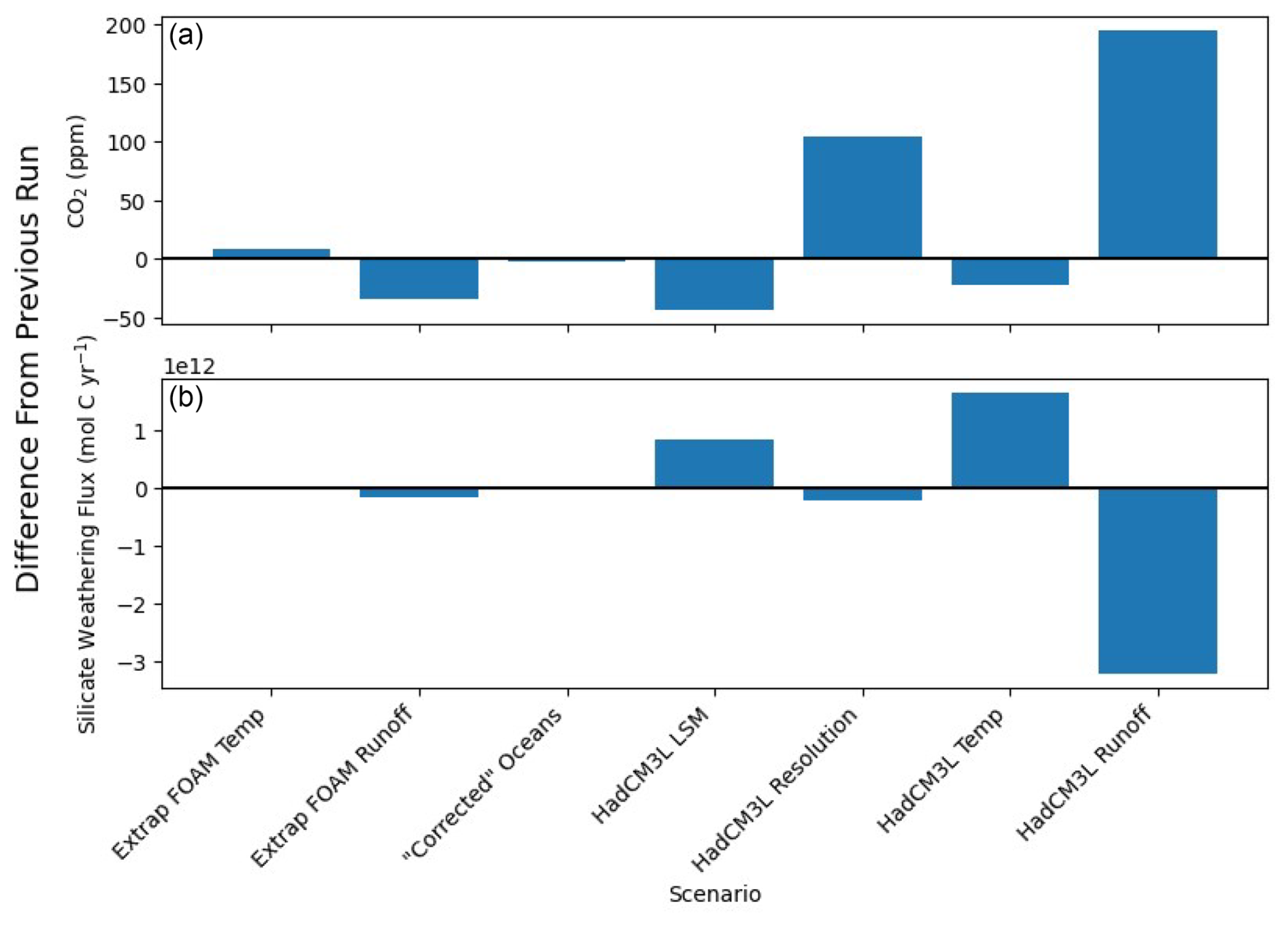
Figure 5 Impact of incremental changes between FOAM and HadCM3L climate inputs in GEOCLIM. (a) Changes in modelled steady-state CO₂ (in ppm; after 1 Myr) for input changes relative to the previous run and (b) changes in global silicate weathering fluxes at CO₂ fixed to 2.85 times the pre-industrial level (mol C yr⁻¹) relative to the previous run. The variable changed in each run is shown as the x axis. Changes in weathering fluxes are essentially an inverse of the pattern of changes in steady-state CO₂.

The step-wise transition between FOAM and HadCM3L revealed that the majority of the differences in steady-state CO₂ concentrations can be explained by differences in model resolution and runoff (Fig. 5), as these produced the greatest changes in steady-state CO₂ values. HadCM3L produces a globally more arid world than the FOAM simulation and shows far greater regional variability. These results are significant, as previous studies (both from field and model data) have suggested that a significant proportion of global weathering fluxes may be the result of so-called “hotspots”, i.e. small land areas with high weathering fluxes such as volcanic islands and mountain ranges (e.g. Kent and Muttoni, 2013). While FOAM inputs show areas of higher runoff associated with mountain ranges, the higher resolution of the HadCM3L inputs relative to FOAM inputs may be sufficient to more accurately resolve weathering hot spots. Furthermore, given that weathering fluxes are highly spatially variable, the HadCM3L simulation likely better constrains such features and thus provides a better estimate of global weathering fluxes. This study indicates a number of areas of high weathering fluxes, particularly outside of the tropics, associated with areas of high relief in the GCM simulations, particularly the Laramide orogeny and Appalachians (North America) and the southern Andes (Fig. 3). In the original HadCM3L simulations, these areas have high runoff rates, likely associated with orographic intensification of rainfall. Thus, the GEOCLIM simulations in this study may provide a better spatial estimate of weathering fluxes than those using FOAM inputs. These regions may be partly responsible for the sharp rise in non-tropical runoff in the Early Cretaceous (Fig. 4) and further support the role of active mountain ranges in influencing CO₂ drawdown (Raymo and Ruddiman, 1992; Riebe et al., 2004; West et al., 2005; Goddéris et al., 2017).

4.4 Implications for palaeoclimates

The GEOCLIM CO₂ concentrations presented in this study reflect the changes in global “weatherability” through the Cretaceous–Eocene period, indicating a general trend towards increased global weatherability during that time, punctuated by a decrease at ∼ 80 Ma (Fig. 6). Although comparison with CO₂ records from proxy data suggests that not all changes in long-term CO₂ can be ascribed to changes in global weatherability, the three records indicate that changes in global weatherability have sufficiently powerful impacts on geologically short timescales (∼ 10 Myr) to be expressed in long-term CO₂ records (i.e. hundreds of ppmv), further supported by the three periods of agreement between the records. These changes in weatherability are primarily associated with the breakup of Pangaea during the Early Cretaceous and with changes in tropical land areas and runoff rates in the mid-Cretaceous and in the Eocene, respectively. Based on these findings, the implications for palaeoclimates are 2-fold.

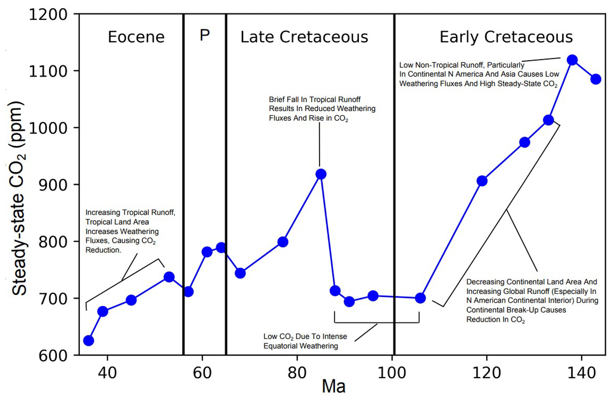
Figure 6 GEOCLIM steady-state CO₂ record with annotations showing major controls on steady-state CO₂ concentrations. Significant changes in steady-state CO₂ are typically due to changes in runoff and continental land areas. Note that Palaeocene has been abbreviated to P.​​​​​​​

Firstly, this study reinforces the conclusions of previous studies that continental configuration is a strong control on long-term CO₂ concentrations by influencing runoff (Otto-Bliesner, 1995; Gibbs et al., 1999; Donnadieu et al., 2004; Goddéris et al., 2014). Supercontinental configurations typically reduce global weatherability and favour high CO₂ concentrations by limiting global runoff, while dispersed configurations typically increase global weatherability and favour lower CO₂ concentrations as the dispersed configuration favours moisture transport to continental interiors.

Secondly, this study demonstrates the potential for relatively localised changes in weatherability to have global impacts. Such local changes may result in a temporary decoupling of globally averaged runoff rates from globally averaged weathering rates. During the Eocene, non-tropical runoff totals fall substantially, but tropical runoff increases significantly, likely associated with an increase in tropical land areas at the same time. Similarly, during the mid-Cretaceous, tropical runoff totals remain stable, but non-tropical rainfall increases. The increase in non-tropical rainfall is sufficient to increase silicate weathering fluxes and lower atmospheric CO₂ concentrations by 200 ppm over 13 Myr.

5 Conclusions

This study explores the potential impact of changing “weatherability” during the Cretaceous–Eocene period on long-term CO₂ concentrations and the impact of using high-resolution GCM data on modelled weathering rates and steady-state CO₂ concentrations. The palaeogeography analysis showed that “weatherability” changed significantly through the Cretaceous–Eocene period as Pangaea broke up and the continents entered a more dispersed configuration. Changes in weatherability as a result of palaeogeographical change are due to two processes. The first process is increased evaporation and more favourable moisture transport as continents became more dispersed, which occurred during the Early Cretaceous. The second process is due to continents moving into more humid zones, which occurred during the late Eocene.

Steady-state CO₂ concentrations were initially high in the Early Cretaceous due to low total global runoff inhibiting weathering fluxes. As Pangaea broke up, evaporation from the ocean increased and improved moisture transport to the continental interiors, increasing runoff rates and weathering fluxes, resulting in lower steady-state CO₂ concentrations. Into the Cenozoic, however, global weatherability appears to switch regimes. In the Cenozoic, weatherability appears to be determined by increases in tropical land area, allowing greater weathering in the tropics. Furthermore, global runoff fell in the late Eocene, but silicate weathering fluxes continued to increase. The increase in silicate weathering is due to an increase in total tropical runoff as land areas in the tropics increased, which is sufficient to allow global weathering fluxes to increase despite a fall in total global runoff.

We also investigated and quantified the impact of using different GCM datasets in GEOCLIM. The high-resolution HadCM3L datasets produced substantially different steady-state CO₂ concentrations relative to FOAM datasets, primarily due to changes in runoff reconstructions. The use of high-resolution GCM data was instrumental in revealing these potential impacts and highlights the benefits of such data in palaeo-weathering studies.

While the aim of this study was to investigate the role of palaeogeography on weatherability, the CO₂ concentrations produced by GEOCLIM were also compared with proxy-derived records from the literature to determine what aspects, if any, of long-term CO₂ change could have been driven by changes in weatherability. Three periods were identified when the GEOCLIM output agreed with the proxy CO₂ records and thus suggest that changes in weatherability were perhaps influencing global climate: the Early Cretaceous, the Late Cretaceous, and the mid-Eocene. High CO₂ concentrations in the Early Cretaceous are likely due to the arid nature of the continental interior. A brief (10–20 Myr) rise in CO₂ during the Late Cretaceous appears to be the result of falling tropical runoff, causing global weathering fluxes to fall. Finally, a falling trend in CO₂ during the mid-Eocene appears to be linked to increased global weatherability as tropical land areas increase.

The periods of agreement with the three CO₂ records indicate that weatherability changes were sufficient in magnitude to affect the long-term climate of the Cretaceous–Eocene period. Furthermore, this study shows the potential for regional changes (e.g. localised changes in tropical runoff and land area) to have global impacts and that such regional changes may be more significant than global averages for determining long-term climate.

Appendix A

Because GEOCLIM interpolates climate variables based on climate data at specified CO₂ concentrations, it was necessary to ensure that both the FOAM and HadCM3L input data had consistent CO₂ concentrations. FOAM was previously run at 11 CO₂ concentrations between 160 and 1400 ppm, while HadCM3L was previously run only at 560 and 1120 ppm. For consistency, a methodology was developed to produce “synthetic” model output from HadCM3L at the same CO₂ concentrations as for FOAM. This was deemed particularly important because GEOCLIM runs with Ypresian FOAM inputs have previously produced CO₂ concentrations below 560 ppm (Lefebvre et al., 2013). In GEOCLIM, if modelled CO₂ concentrations exceed the available CO₂ range, the climate variables will cease to update.

To address these issues, the HadCM3L climate inputs were extrapolated to the same 11 CO₂ concentrations to cover the same range as the FOAM data. Two separate extrapolation methods were used to calculate the temperature and runoff to better reflect their sensitivity to CO₂ concentration changes in observed data. The HadCM3L temperature (T_x) for a CO₂ concentration of CO_2x was approximated as

$$\begin{array}{}\text{(A1)}& T_x=T_{\mathrm{560}}+\left(T_{\mathrm{diff}}\times {\displaystyle \frac{\ln \frac{{\mathrm{CO}}_{\mathrm{2}x}}{\mathrm{280}}}{\ln \mathrm{2}}}-\mathrm{1}\right).\end{array}$$

Temperature values were extrapolated based on absolute differences between the 560 and 1120 ppm temperature outputs (Eq. A1). T_x is the temperature value at any given CO₂ concentration, where T₅₆₀ is the temperature at 560 ppm, T_diff is the difference in temperature between 1120 and 560 ppm, and CO_2x is a specific concentration of atmospheric CO₂ (ppm).

Runoff was extrapolated in a similar fashion to temperature, except that a constant ratio rather than a constant absolute difference was assumed per CO₂ doubling, because this relationship is found in the model results and because absolute value changes would result in large areas of negative runoff and excessive aridity at lower CO₂ concentrations which were deemed to be unrealistic:

$$\begin{array}{}\text{(A2)}& R_x=R_{\mathrm{560}}\times \exp \left({\displaystyle \frac{{\mathrm{CO}}_{\mathrm{2}x}-\mathrm{560}}{\mathrm{560}}}\times \ln \left(R_{\mathrm{diff}}\right)\right).\end{array}$$

Equation (A2) was used to extrapolate runoff rates (cm yr⁻¹), R_x, at any given CO₂ concentration. R₅₆₀ represents the runoff rate at 560 ppm, while R_diff is the magnitude difference between runoff values at 1120 and 560 ppm.

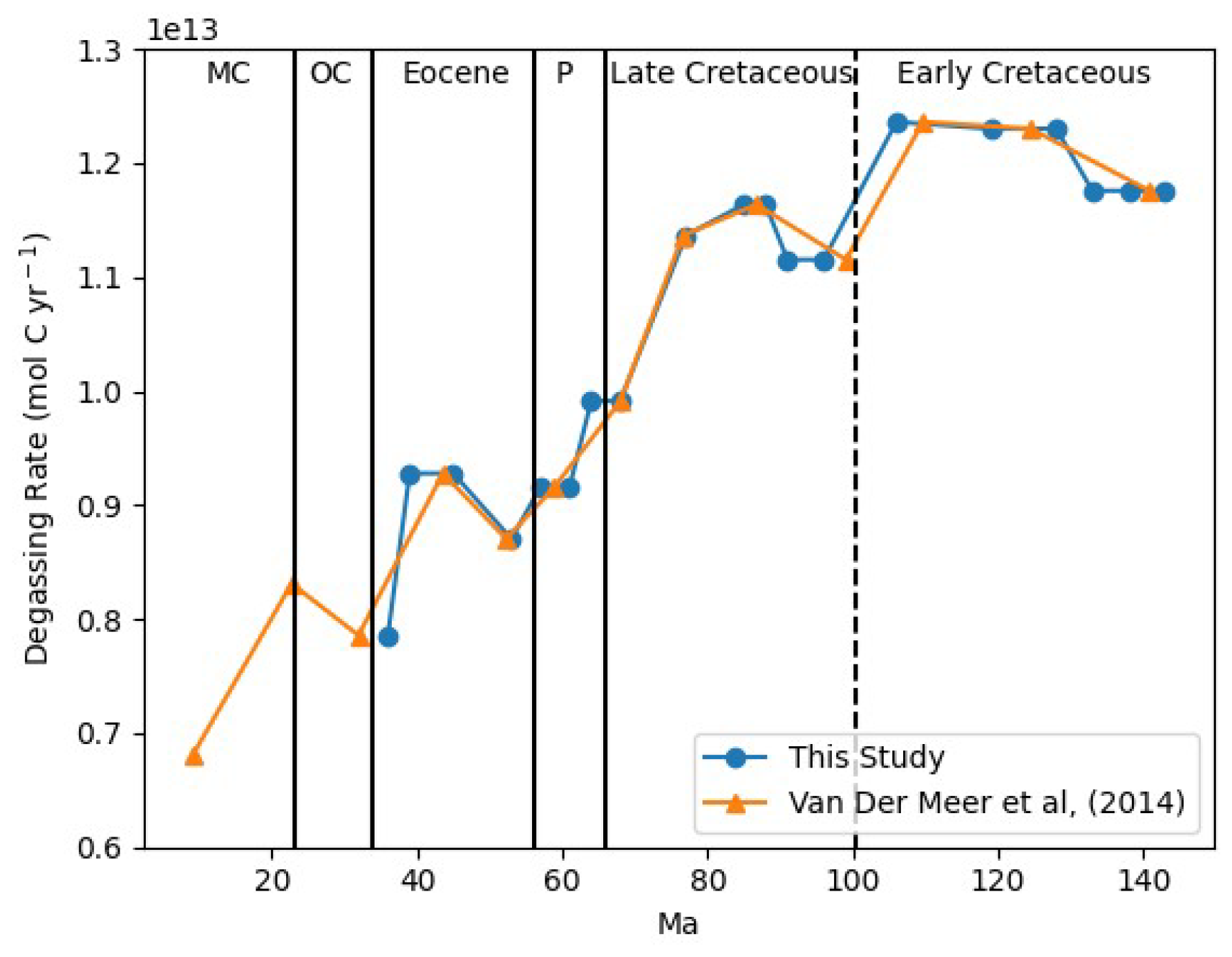
Figure A1 Degassing rates from Van Der Meer et al. (2014) (blue) used to provide variable degassing rates for the 19 time slices used in this study (green). Each time slice uses the rate from Van Der Meer et al. (2014) that is nearest in time. Degassing rates are highest in the Early to mid-Cretaceous (110–130 Ma) and gradually fall into the Paleogene, with occasional rises. MC: Miocene; OC: Oligocene; P: Palaeocene.

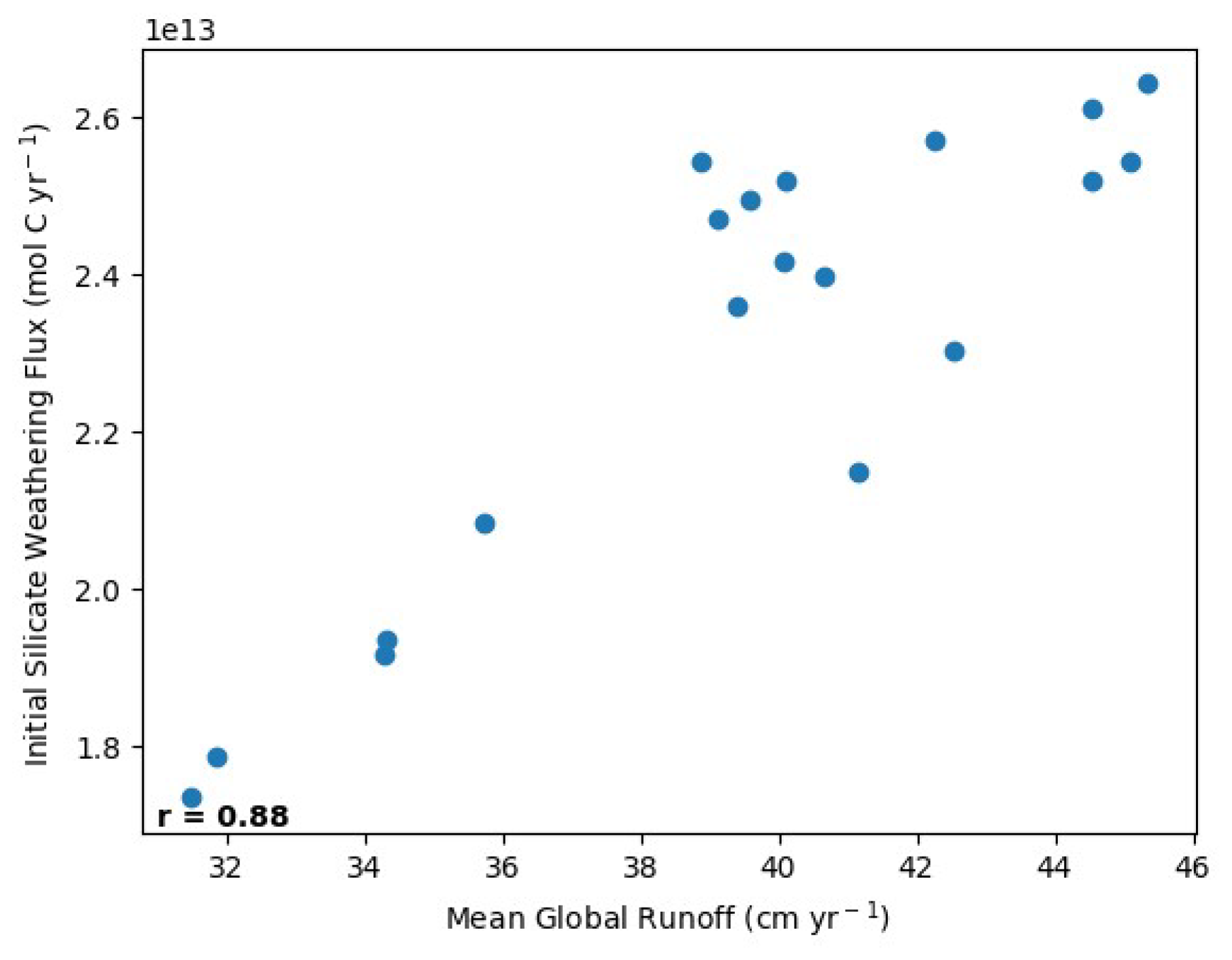
Figure A2 Scatter plot of mean global runoff and initial silicate weathering fluxes from the 19 modelled time slices. Global runoff and silicate weathering fluxes show a strong positive correlation (R=0.88).

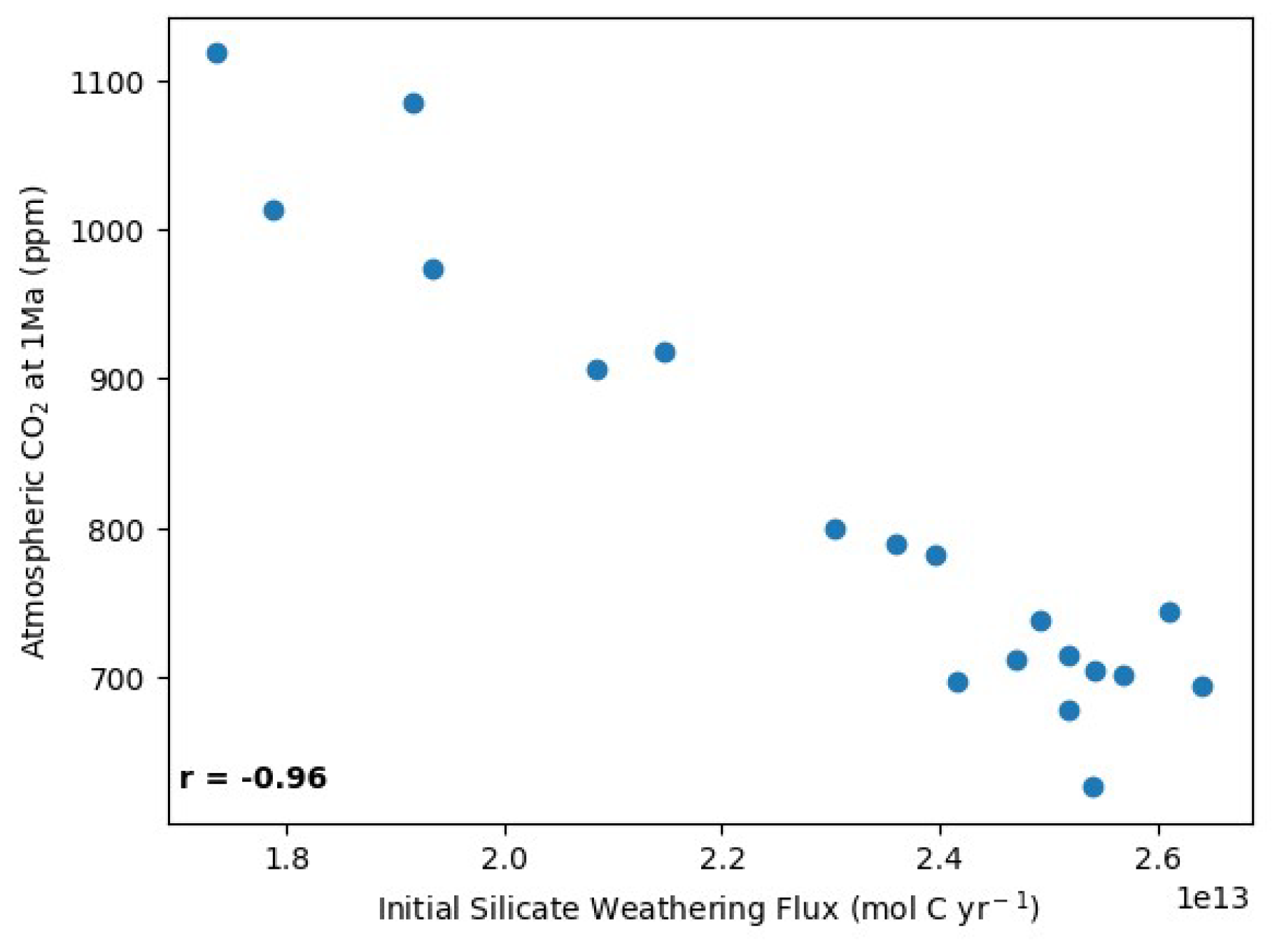
Figure A3 Scatter plot of initial silicate weathering fluxes and steady-state atmospheric CO₂ concentrations from the 19 modelled time slices. Silicate weathering fluxes and steady-state atmospheric CO₂ concentrations show a very strong negative correlation ($R=-\mathrm{0.96}$).

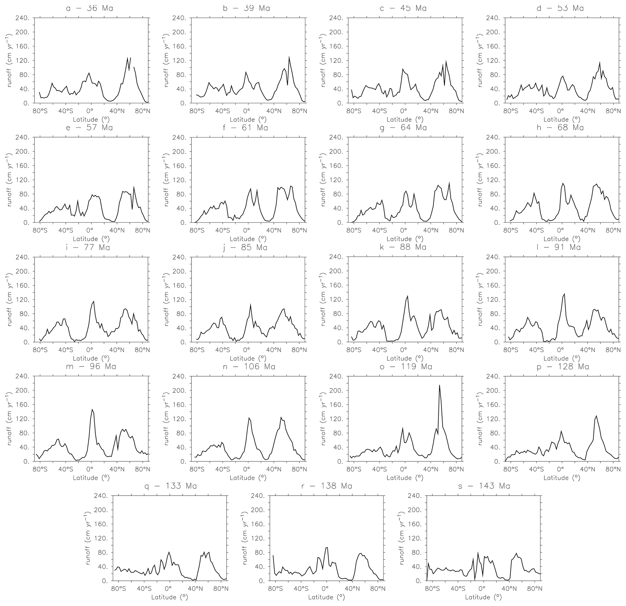
Figure A4 Modelled zonal mean runoff (cm yr⁻¹) from the earliest Cretaceous (s) to the latest Eocene (a). Zonal runoff means are low in the Early Cretaceous (s–p) but increase significantly into the mid-Cretaceous, especially in the northern mid-latitudes (o–k). Zonal mean runoff falls slightly into the Late Cretaceous, but there is an intensification in equatorial mean zonal runoff (j–h). In the Cenozoic, zonal runoff intensifies again (g–e) but begins to weaken again during the Eocene (d–a).