Ice core site considerations from modeling CO₂ and O₂ ∕ N₂ ratio diffusion in interior East Antarctica

Obtaining a continuous ice core record to 1.5 Ma (million years), which spans the Mid-Pleistocene Transition (MPT, 1.2 to 0.7 Ma) is a goal of multiple international efforts in Antarctica. Ice of such age is likely to be highly thinned and located in warm ice near the bed, conditions which promote diffusion of the stored atmospheric gases. Here, we assess the preservation of CO₂ and the O₂ $/$ N₂ ratio in the ice sheet between South Pole and Dome A where the NSF Center for Oldest Ice Exploration has surveyed with airborne radar. We employ two models: (1) a 1D, steady state ice and heat flow model to calculate the temperature and age of ice with respect to depth, and (2) a vertical gas diffusion model for clathrate ice. We analyze the preservation of CO₂ signals with a period of 40 kyr to match pre-MPT glacial cycles and the preservation of O₂ $/$ N₂ signals with a period of 20 kyr to match precession cycles. 1.5 Ma ice is lost to basal melt in much of the study area where ice thickness exceeds 3000 m. In locations that preserve 1.5 Ma ice, vertical gas diffusion is most sensitive to accumulation rate; high accumulation rate sites have more highly thinned old ice, and the steeper gas concentration gradients enhance diffusion. The most promising region for recovering 1.5 Ma ice is approximately 400 km from both South Pole and Dome A, a region we call the “Foothills”, due to low accumulation rates and moderate ice thickness. CO₂ signals lose on average 14 % of their amplitude, while O₂ $/$ N₂ signals lose on average 95 % for 1.5 Ma ice, suggesting precession cycles may not be identifiable. Unknown geothermal heat flow is a large uncertainty for both ice loss from basal melt and gas signal preservation.

1 Introduction

Extending the continuous ice core record through the Mid-Pleistocene Transition (MPT) to ∼1.5 Ma (million years) is a goal of the International Partnership in Ice Core Sciences (Fischer et al., 2013). The MPT is a climatic transition that occurred between 1.2 and 0.7 Ma during which Earth's glacial cycles shifted from high frequency (∼40 kyr – thousand years), low amplitude events to low frequency (∼100 kyr), high amplitude events (Head et al., 2008). The MPT has been observed in the benthic δ¹⁸O record (Fig. 1, top panel), a climate proxy used to estimate global ice volume (Lisiecki and Raymo, 2005); the cycle transition was first noted by Shackleton and Opdyke (1976). The mechanisms underlying the MPT are not fully understood (Clark et al., 2006; Tziperman and Gildor, 2003; Rial et al., 2004). The role of a proposed gradual decline in atmospheric CO₂ remains an open question (Hönisch et al., 2009; Martin et al., 2024). Atmospheric CO₂ concentrations prior to the ice core record limit (0.8 Ma; EPICA community members, 2004) have been reconstructed using δ¹¹B derived from planktic foraminifera (Bartoli et al., 2011; Chalk et al., 2017; de la Vega et al., 2020; Dyez et al., 2018; Guillermic et al., 2022; Henehan et al., 2013; Hönisch et al., 2009; Martínez-Botí et al., 2015; Seki et al., 2010). However, this method is limited, providing different results based on the species and location and requiring several assumptions. Köhler (2023) suggests that some of these assumptions, such as equilibrium between atmospheric and equatorial sea surface pCO₂, lower estimated surface ocean pH in the Pacific than the Atlantic, and assumptions on total alkalinity and dissolved inorganic carbon, may be incorrect by comparing reconstructions to a carbon cycle model. Therefore, answering questions regarding atmospheric CO₂ concentration's role in the MPT may require direct measurements from an ice core older than 0.8 Ma.

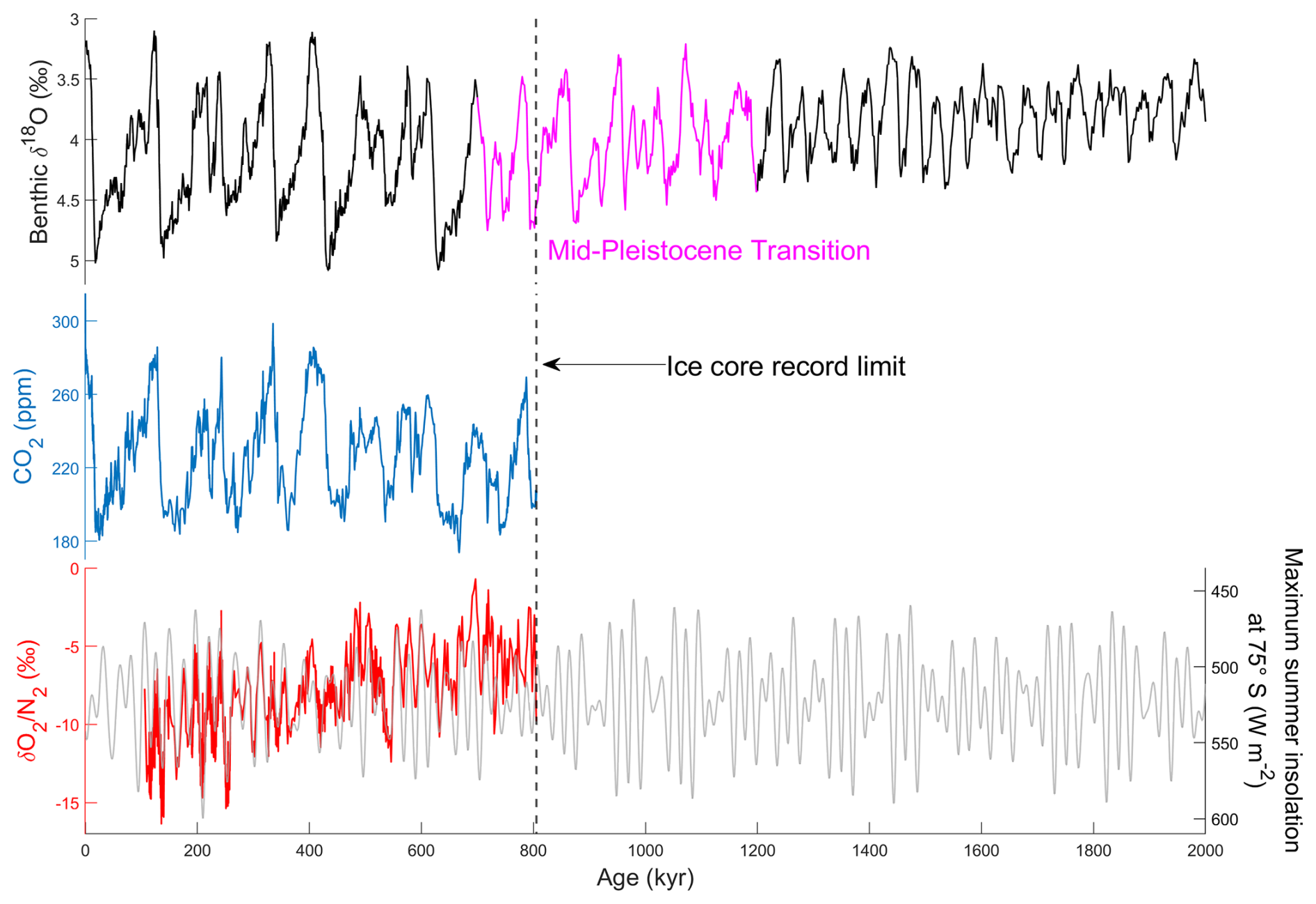
Figure 1 Top: record of benthic δ¹⁸O, a proxy for global ice volume, from the LR04 Stack (Lisiecki and Raymo, 2005). The MPT (top magenta) is the transition from low amplitude, high frequency glacial cycles to high amplitude, low frequency cycles. The ice core record of CO₂ (middle: Ahn et al., 2012; Bereiter et al., 2015; Lüthi et al., 2008; Indermühle et al., 2000; Siegenthaler et al., 2005; see National Centers for Environmental Information, 2023: Antarctic Ice Cores Revised 800 kyr CO₂ Data website for data) does not cover the full MPT. An extended ice core record of CO₂ back to 1.5 Ma may provide insights about the MPT. The O₂ $/$ N₂ ratio in the ice core record (bottom red; Bouchet et al., 2023b; see Bouchet et al., 2023a for data), which has been observed to follow maximum summer insolation at 75° S (bottom grey; Berger, 1978; Berger and Loutre, 1991). This can be used for dating an extended ice core by matching precession cycles in the O₂ $/$ N₂ ratio. Time axis is inverted for all plots.

The National Science Foundation Center for Oldest Ice Exploration (NSF-COLDEX) is investigating the area between the South Pole and Dome A to identify a drill site for a continuous deep ice core reaching 1.5 million years (Young et al., 2025a). Ice of this age will have thinned significantly, steepening gas concentration gradients. Furthermore, it will have experienced a long duration of warm temperatures near the bed, increasing the diffusivity and solubility of the gases. Thus, both steeper gradients and warmer temperature promote diffusive smoothing in trapped gases that may inhibit recovery of atmospheric gas records, where 1.5 Ma ice is recovered.

In this study, we assess the preservation of atmospheric gas signals in 1.5-million-year-old ice. We first model the depth-age and temperature profiles in the COLDEX study area and then model the diffusion of CO₂ and the O₂ $/$ N₂ ratio. We analyze the effects of accumulation rate, ice thickness, surface temperature, and geothermal heat flow (GHF) on gas signal preservation.

Accumulation rate has opposing effects on gas signal preservation. High accumulation rates advect cold surface temperatures deeper into the ice column, leading to a cooler temperature profile. On the other hand, high accumulation rates lead to increased thinning in near-basal ice layers, where old ice is present, and thus increases gas concentration gradients. Ice thickness also has opposing effects on gas signal preservation. Thicker ice columns cause less thinning, allowing for thicker layers and less steep gradients in near-basal ice. However, a thick ice column also increases the basal temperature and leads to more basal melt, potentially removing the oldest ice. Surface temperature and GHF are boundary conditions for the temperature profile, so lower values will result in a cooler temperature profile. Moreover, minimizing near-basal temperatures will mitigate the basal melt rate, increasing the likelihood that old ice is present.

We focus on CO₂ and the O₂ $/$ N₂ ratio in this study. CO₂ is an important paleoclimate parameter (Ahn et al., 2012; Bereiter et al., 2015; Lüthi et al., 2008; Indermühle et al., 2000; Siegenthaler et al., 2005). Long-term cooling, often attributed to an assumed secular decrease in atmospheric pCO₂, is at the heart of many possible explanations for the MPT (Raymo et al., 1997; Mudelsee and Schulz, 1997; Berger et al., 1999). The O₂ $/$ N₂ ratio is an important dating tool (Kawamura et al., 2007; Bouchet et al., 2023a) because it records precession cycles by tracking maximum summer insolation, due to influences on snow metamorphism and grain properties in shallow firn (Martinerie et al., 1992; Bender et al., 1994, 1995; Bender, 2002; Kawamura et al., 2007; Fujita et al., 2009; Lipenkov et al., 2011). This is a key method in dating gases in the oldest ice cores (Oyabu et al., 2022). Histories of these gases from the current ice core record can be found in Fig. 1.

We build upon the work of Bereiter et al. (2014) where the preservation of CO₂ and the O₂ $/$ N₂ ratio is evaluated for an idealized ice core location. Here, we similarly evaluate signal preservation using the new information provided by the NSF-COLDEX airborne survey (Young et al., 2025a). We limit our discussion of CO₂ and the O₂ $/$ N₂ ratio to the periods of 40 and 20 kyr, respectively, to match pre-MPT glacial cycles for CO₂ and precession cycles for the O₂ $/$ N₂ ratio. Bereiter et al. (2014) modeled O₂ $/$ N₂ diffusion under two sets of gas parameter values, a “fast set” after Ikeda-Fukazawa et al. (2005) and a “slow set” after Salamatin et al. (2001). Here, we consider only the “slow set” due to the unrealistic modeling results obtained by Oyabu et al. (2021) when using the fast set parameters (Sect. 2.3).

2 Methods

The diffusive smoothing that atmospheric signals stored in the ice sheet have experienced depends on both the temperature history of the ice and the gradient in gas concentrations. These parameters are determined by the time-evolving depth-age relationship. In this section, we first describe the study area and data sources for model forcings. We then describe a one-dimensional, steady-state model of ice and heat flow (Fudge et al., 2019; Firestone et al., 1990; Lliboutry, 1979). This model is used to provide the physical parameters for a gas diffusion model (Bereiter et al., 2014).

2.1 Study area

The COLDEX study area is divided into three regions based loosely on the ice thickness and its variability (Fig. 2):

• Foothills – upstream-most portion of the survey towards Dome A with variable ice thickness that typically ranges from ∼2500 to ∼3000 m.

• Deep basin – the middle of the survey area where ice thickness typically exceeds ∼3000 m.

• Saddle region — the region upstream from South Pole where ice thickness becomes more moderate, ∼2000 to ∼3000 m, and the ice flow diverges.

The accumulation rates across the study area are inferred from an englacial layer dated to 4.7 ka and given in ice equivalent (Fudge, 2025). Because we use a steady-state model, we scale the inferred accumulation rate for the past 4.7 ka to the long-term (past four glacial cycles, 450 ka) average at Dome C using the AICC2012 chronology (Bazin et al., 2013; Veres et al., 2013). The average accumulation rate for the past 4.7 ka is 2.9 cm yr⁻¹ and for the past 450 ka is 2.1 cm yr⁻¹. This gives a factor of 0.72. Figure 8a shows the accumulation rate across the study area. Surface temperatures, which also approximate a glacial-cycle average, are interpolated across the region based on the easting from the South Pole, with the warmest temperatures, −54 °C, at the South Pole, cooling linearly to the grid-east to the Dome A foothills, reaching −60 °C at the end of the study area (Fig. 8c). We chose −54 °C at the South pole from a rough time weighted average temperature between glacial and interglacial periods (Buizert et al., 2021; Kahle et al., 2021) and −60 °C at the foothills assuming a combination of lapse rate from the 800 m elevation gain from the South Pole and warmer northward temperatures. GHF is poorly known in the study region because there are no direct measurements. Remotely sensed estimates (Stål et al., 2020; Shen et al., 2020; An et al., 2015; Maule et al., 2005; Martos et al., 2017; Shapiro and Ritzwoller, 2004; Purucker et al., 2013; Hazzard and Richards, 2024) vary widely (e.g. Van Liefferinge et al., 2018). Therefore, we assume a uniform GHF across the study area and consider a range of values to assess how uncertainty in GHF values may affect near-basal ice age, melt rate, and signal diffusion.

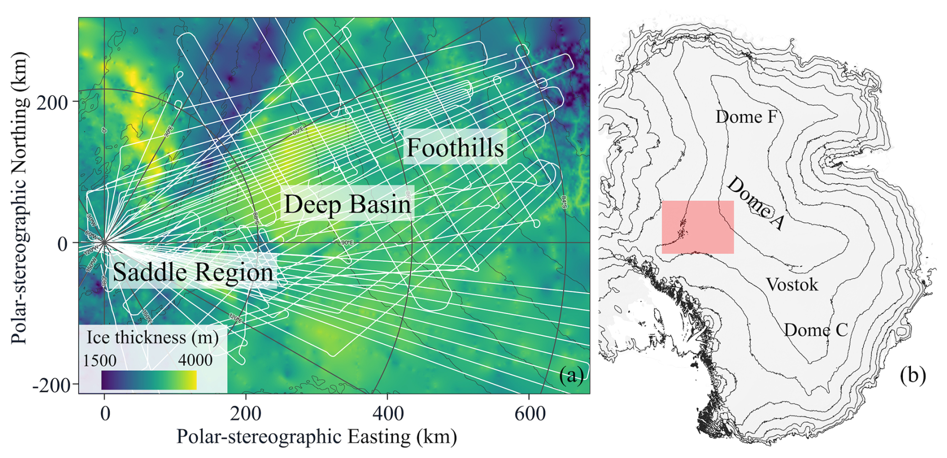
Figure 2 (a) COLDEX study area and sub-regions used for this study, defined loosely on ice thickness (see Young et al., 2025a, and Bedmap3 for data; Pritchard et al., 2025). White lines indicate flight paths. Grey contour lines represent 100 m elevation change (see REMA v2 for data; Howat, 2022). (b) Map of East Antarctica. The red rectangle represents the study area. Contour lines represent 500 m elevation change.

2.2 Temperature and age-depth model

We use a one-dimensional, steady state ice and heat flow model to calculate the temperature and age of ice with respect to depth. The age model is identical to that in Bereiter et al. (2014). The temperature model differs in that we utilize a temperature dependent thermal conductivity and specific heat capacity, rather than an ice column average. If the basal temperature exceeds the pressure melting point, the melt rate is calculated. We choose a steady-state model because the conditions near the base of the ice sheet, where the vast majority of diffusion occurs, are relatively insensitive to the transient surface climate forcing. In a set of ice flow model runs, glacial-interglacial changes in surface temperature of 8 °C results in a difference in basal temperature of <0.5 °C (Buizert et al., 2021). This model utilizes input parameters of accumulation rate, ice thickness, surface temperature, GHF, and a parameter for the vertical deformation profile (Lliboutry, 1979). Figure 3a–d show an example output of this model using forcings of 2 cm yr⁻¹ accumulation rate, 3000 m ice thickness, −60 °C surface temperature, 50 m W m⁻² GHF, and a vertical deformation parameter of p=4.

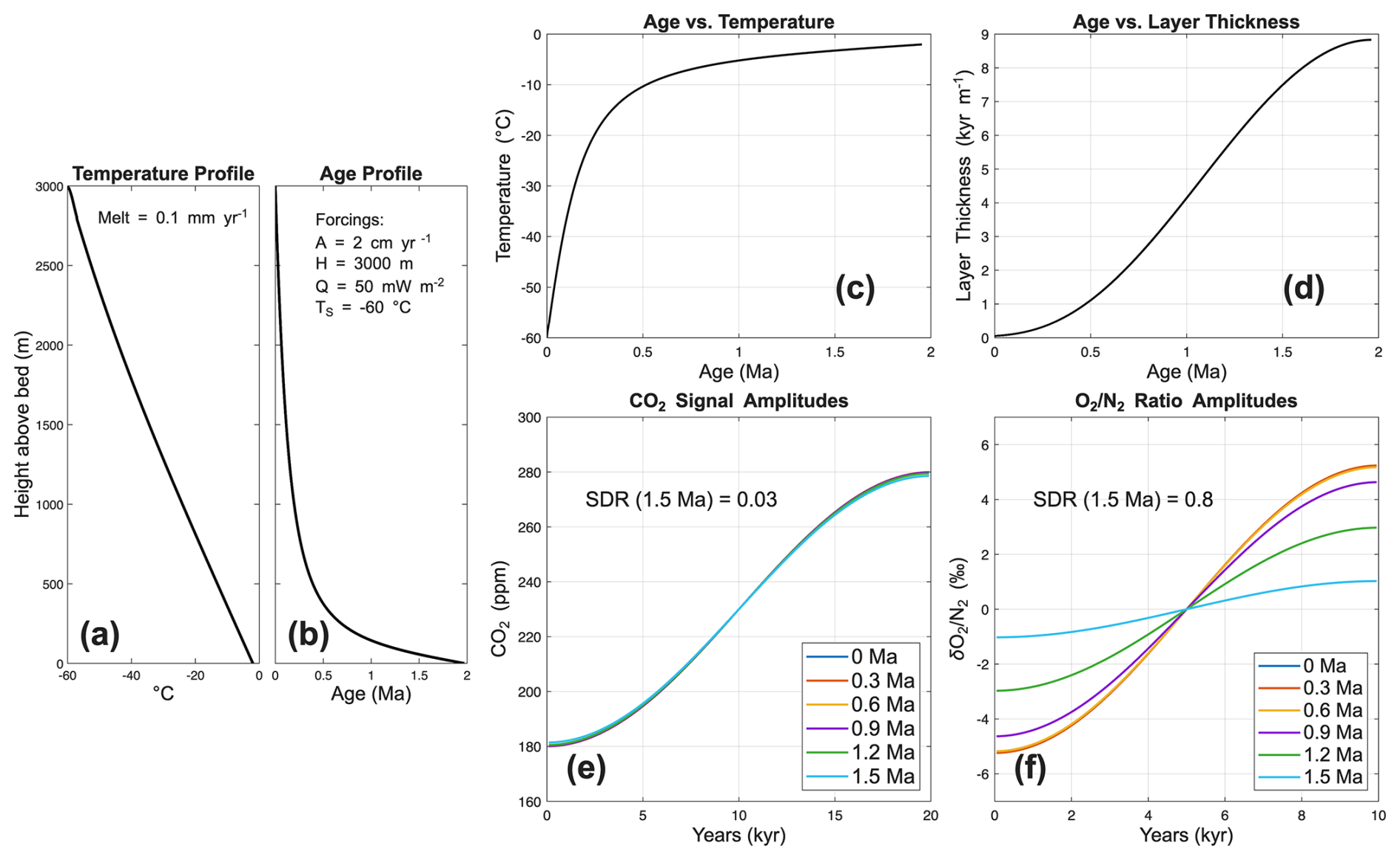
Figure 3 Example output from models using forcings of 2 cm yr⁻¹ accumulation rate, 3000 m ice thickness, 50 m W m⁻² GHF, and −60 °C surface temperature. (a) Temperature and (b) age profile calculated with 1D, steady state model. c) Age-temperature relationship. (d) Age-layer thickness relationship. (e) CO₂ and (f) O₂ $/$ N₂ ratio amplitude evolution through time. SDR represents the fraction of gas signal lost. In this example, CO₂ loses very little signal amplitude, only 3 % as indicated by the SDR. The O₂ $/$ N₂ ratio loses much more signal, 80 % by 1.5 Ma, but only begins losing its amplitude around 0.9 Ma.

The steady heat equation, following Firestone et al. (1990), is solved to obtain the vertical temperature profile:

$$\begin{array}{}\text{(1)}& {\displaystyle \frac{{\partial }^{\mathrm{2}}T}{\partial z^{\mathrm{2}}}}-{\displaystyle \frac{w\left(z\right)}{\mathit{\kappa }}}{\displaystyle \frac{\partial T}{\partial z}}=\mathrm{0},\end{array}$$

where T is temperature, z is height above the bed. The thermal diffusivity is given by $\mathit{\kappa }=\frac{K}{\mathit{\rho }c}$, where ρ is the constant firn column density based on South Pole values (Lilien et al., 2018), c is the temperature-dependent specific heat capacity given by Cuffey and Paterson (2010; Eq. 9.1), and k is the thermal conductivity exponentially fit to the Waite et al. (2006) data as described in the supplementary information of Buizert et al. (2021) (Specific values can be found in the setup_thermal_herc.m file in the GitHub repository). w is the vertical velocity as calculated by Parrenin et al. (2007):

$$\begin{array}{}\text{(2)}& {\displaystyle }& {\displaystyle }w\left(z\right)=-(A-m)\mathit{\psi }\left(z\right)m,\text{(3)}& {\displaystyle }& {\displaystyle }\mathit{\psi }\left(z\right)=\mathrm{1}-{\displaystyle \frac{p+\mathrm{2}}{p+\mathrm{1}}}\left(\mathrm{1}-{\displaystyle \frac{z}{H}}\right)+{\displaystyle \frac{\mathrm{1}}{p+\mathrm{1}}}{\left(\mathrm{1}-{\displaystyle \frac{z}{H}}\right)}^{p+\mathrm{2}},\end{array}$$

where A is accumulation rate, H is ice thickness, and p is a tuning parameter for vertical deformation (Lliboutry, 1979). The deformation parameter is assumed to be p=4 in all scenarios, unless otherwise stated. We include the bedrock in the thermal calculation and set the GHF at 7 km below the ice surface. The melt rate, m, is first set at 0 for calculating the temperature profile. Equation (1) is solved similarly to Firestone et al. (1990) with an integration factor:

$$\begin{array}{}\text{(4)}& F\left(z\right)=\exp \left[-\underset{\mathrm{0}}{\overset{z}{\int }}{\displaystyle \frac{w\left(\mathit{\zeta }\right)}{\mathit{\kappa }}}\mathrm{d}\mathit{\zeta }\right].\end{array}$$

This gives the following solution:

$$\begin{array}{}\text{(5)}& T\left(z\right)=T_{\mathrm{S}}-{\displaystyle \frac{Q}{K}}\underset{H}{\overset{z}{\int }}{\displaystyle \frac{\mathrm{1}}{F\left(\mathit{\eta }\right)}}\mathrm{d}\mathit{\eta }.\end{array}$$

where T_S is the surface temperature and Q is GHF. The melt rate is calculated from the excess geothermal heat that the ice cannot conduct away from the bed. This is calculated iteratively because the melt rate affects the vertical velocity (Eq. 2) and thus the englacial temperature profile. The GHF is equal to the heat conduction through the basal ice and the latent heat lost in melting, which we assume is lost as the water flows away from the bed. The example temperature profile in Fig. 3a shows how temperature increases roughly linearly with depth approaching the bed as a result of this solution.

The vertical age profile is found by solving Eqs. (2) and (3) with the inferred melt rate and integrating the inverse of the negative vertical velocity:

$$\begin{array}{}\text{(6)}& \mathrm{age}\left(z\right)=\int {\displaystyle \frac{-\mathrm{1}}{w\left(z^{\prime }\right)}}\mathrm{d}{z}^{\prime }.\end{array}$$

The example age-depth profile in Fig. 3b shows how the age of ice evolves with depth up to 2 Ma, after which older ice has been melted by the warm temperatures shown in Fig. 3a.

2.3 Gas diffusion model

The gas diffusion model uses the temperature- and age-depth profiles described above to calculate the rate of diffusion through time (Ikeda-Fukazawa et al., 2005; Bereiter et al. 2014). Vertical gas diffusion is modeled as follows:

$$\begin{array}{}\text{(7)}& {\displaystyle \frac{\partial C_n}{\partial \mathrm{t}}}={\displaystyle \frac{\partial }{\partial z}}\left(D_n{\displaystyle \frac{\partial C_n}{\partial z}}\right),\end{array}$$

where C_n is the concentration in the ice of n (CO₂ or O₂) and D_n is the diffusion coefficient in ice. Gas exchange with surrounding ice is calculated according to Ikeda-Fukazawa et al. (2005) and Bereiter et al. (2009). The model does not include a portion for diffusion in bubbly ice and instead treats the whole ice column as clathrate ice for simplicity. While diffusion does occur within bubbly ice, the time gases spend in the bubble phase is relatively short compared to the timescales of interest here (e.g. ice 1000 m below the surface at EDC is ∼65 ka, roughly the extent of bubbly ice; Bazin et al., 2013; Veres et al., 2013). We only simulate the diffusion of O₂ because N₂ has a permeation coefficient roughly one order of magnitude lower than that of O₂ (Salamatin et al., 2001). Modeling O₂ diffusion is sufficient for modeling the damping of the O₂ $/$ N₂ ratio. Including N₂ diffusion would reduce the smoothing of δO₂ $/$ N₂ from O₂ diffusion, provided that the gas concentration gradient of N₂ has the same sign as O₂. This condition is likely met as millennial-scale variable of δO₂ $/$ N₂ and total air content in ice is thought to be driven by similar bubble-closure processes. This is supported by empirical data showing δO₂ $/$ N₂ and total air content covariance (Fujita et al., 2009; Lipenkov et al., 2011). Thus, this study provides an upper limit on δO₂ $/$ N₂ smoothing in ice cores. Note that if O₂ and N₂ gas concentration gradients were of opposite signs, the effects of their diffusion would be additive and thus enhance smoothing.

The concentration of dissolved molecules of gas in pure clathrate ice, C_n, is calculated as follows:

$$\begin{array}{}\text{(8)}& C_n=Z_n\cdot P_n^{\mathrm{d}}\cdot S_n,\end{array}$$

where Z_n is the molar fraction of gas n in air enclosed in the clathrate, $P_n^{\mathrm{d}}$ is the clathrate dissociation pressure of gas n, and S_n is the solubility of gas n. The clathrate dissociation pressure is species and temperature dependent, and has been experimentally determined (O₂: Kuhs et al., 2000; CO₂: Miller, 1961).

$$\begin{array}{}\text{(9)}& {\log }_{\mathrm{10}}{P}_n^{\mathrm{d}}=a_n-{\displaystyle \frac{b_n}{T}},\end{array}$$

where T is the temperature in Kelvin.

After Bereiter et al. (2014), we use solubility and diffusivity parametrizations from Ahn et al. (2008) and Salamatin et al. (2001) for CO₂ and O₂, respectively. Diffusive smoothing is dependent on the product of diffusivity and solubility: permeability. Permeability values in clathrate ice are difficult to measure in a lab setting due to their extremely small values, so they are instead indirectly estimated based on a model which simulates air fractionation and diffusive smoothing in an ice core. The coefficients for CO₂ have experimental support at 250 K and are further extrapolated (Ahn et al., 2008). This is the only reliable estimate available for CO₂ permeability, based on an analysis of refrozen melt water in the Siple Dome ice core; however, these estimates have not been independently experimentally verified. Bereiter et al. (2014) modeled O₂ $/$ N₂ diffusion under two sets of gas parameters, a “fast set” and “slow set”. The “slow set” parameters are derived from empirical fits to ice core data (Salamatin et al, 2001). The “fast set” parameters are based purely on molecular dynamics simulations of gas diffusion in ice (Ikeda-Fukazawa et al., 2004). The values for the “fast set” and the “slow set”, as well as for CO₂ permeability, can be found in Fig. S1 in the Supplement. Oyabu et al. (2021) demonstrates that the “fast set” parameters yield unrealistically high rates of smoothing compared to high resolution O₂ $/$ N₂ measurements from the Dome Fuji core (DF1). Thus, we utilize the “slow set” in this study. For all gases, the permeation coefficients increase as temperature increases, with O₂ increasing more rapidly than CO₂, but their true sensitivity to temperature is not well known.

Within the gas diffusion model, we calculate the diffusivity as follows:

$$\begin{array}{}\text{(10)}& D_n\left(T\right)=D_n^{\mathrm{0}}\exp \left(-{\displaystyle \frac{Q_n}{R\cdot T}}\right),\end{array}$$

where Q_n is the activation energy for the diffusion coefficient of molecules of gas n in ice D_n(T), R is the ideal gas constant, T is the temperature, and $D_n^{\mathrm{0}}$ is a specific constant for each gas (Bereiter et al., 2009; Ikeda-Fukazawa et al., 2005). For CO₂, we calculate solubility as follows:

$$\begin{array}{}\text{(11)}& S_{{\mathrm{CO}}_{\mathrm{2}}}\left(T\right)=S_{{\mathrm{CO}}_{\mathrm{2}}}^{\mathrm{0}}\exp \left(-{\displaystyle \frac{E_{{\mathrm{CO}}_{\mathrm{2}}}}{R\cdot T}}\right),\end{array}$$

where $E_{{\mathrm{CO}}_{\mathrm{2}}}$ is the activation energy for the temperature dependent solubility $S_{{\mathrm{CO}}_{\mathrm{2}}}\left(T\right)$ and $S_{{\mathrm{CO}}_{\mathrm{2}}}^{\mathrm{0}}$ is a specific constant (Bereiter et al., 2009). To calculate solubility for O₂, we first calculate the permeability:

$$\begin{array}{}\text{(12)}& P_{{\mathrm{O}}_{\mathrm{2}}}\left(T\right)=\left[P_{{\mathrm{O}}_{\mathrm{2}}}^{\mathrm{0}}\exp \left(-{\displaystyle \frac{Q_{\mathrm{P}}}{R\cdot T}}\right)\right]/P_{\mathrm{diss}}^{\mathrm{220}\mathrm{K}},\end{array}$$

where Q_P is the activation energy for permeation, $P_{{\mathrm{O}}_{\mathrm{2}}}^{\mathrm{0}}$ is a specific constant (Salamatin et al., 2001), and $P_{\mathrm{diss}}^{\mathrm{220}\mathrm{K}}$ is the dissociation pressure of O₂ evaluated at 220 K, as in Eq. (9). Solubility is then solved as the quotient of the permeability and diffusivity.

The ice column is partitioned into discrete intervals of 50 kyr of ice age. An ice particle being advected down the ice column spends 50 kyr in each interval. An average annual layer thickness and average temperature are calculated for each interval. Gas concentrations are initialized, and the model simulates diffusion based on the properties of the first 50 kyr interval. Next, gas concentrations are saved, and the model physical parameters are updated using the average layer thickness and temperature from the next interval. Then, the simulation continues for the next 50 kyr interval. The process iterates until the last interval is reached (e.g. Fig. 3e and f).

We use a 40 kyr period for CO₂ to match the predicted frequency of glacial cycles prior to the MPT and a 20 kyr period for the O₂ $/$ N₂ ratio to match precession cycles. To express the amount of signal amplitude lost to diffusion, we define the signal damping ratio (SDR) as:

$$\begin{array}{}\text{(13)}& \mathrm{SDR}\left(\mathrm{age}\right)=\mathrm{1}-{\displaystyle \frac{X\left(\mathrm{age}\right)}{X\left(\mathrm{0}\right)}},\end{array}$$

where X(age) is the gas signal amplitude at a given age and X(0) is the initial gas signal amplitude. We use an initial amplitude of 50 ppm for CO₂ and 5 ‰ for the O₂ $/$ N₂ ratio. The SDR gives the fraction of gas signal lost at a target age, with higher values indicating more diffused gas signals. The SDR for 1.5 Ma will be of most interest in this study as it fully covers the MPT and some time prior to it. Figure 3e and f shows how CO₂ and O₂ $/$ N₂ ratio concentrations evolve through time given the corresponding temperature- and age- depth profiles. CO₂ signal amplitudes do not change significantly in this example (Fig. 3e). O₂ $/$ N₂ ratio signal amplitudes dampen in old ice, particular in ice older than 0.9 Ma (Fig. 3f).

3 Results

We conduct three sets of simulations with the gas diffusion model. First, we force the model with physical parameters from EPICA Dome C and Dome Fuji to assess whether the existing ice core record can be used to predict the expected diffusion in older records. Second, we assess the sensitivity of each gas's SDR to the four model input parameters to gain an intuition of which forcings are most important. Third, we run the model over the NSF-COLDEX study area to understand where old ice may reside in the region and where each gas will be best preserved.

3.1 Diffusion in existing ice core records

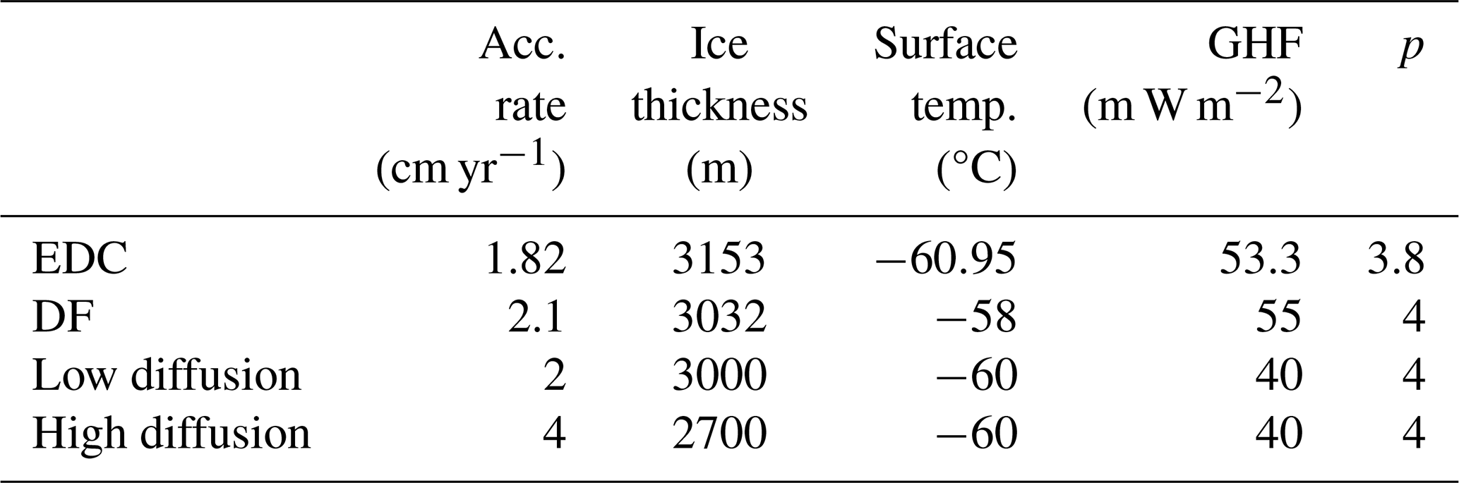
To determine the extent to which ice core gas concentration measurements can be used to estimate the expected diffusion of atmospheric gases in 1.5 Ma ice, we conduct four model runs. In the first run, we simulate the conditions for EPICA Dome C (EDC) and use parameter values from Bereiter et al. (2014) (“EDC” in Table 1). In the second run, we simulate the conditions for Dome Fuji with parameters values tuned to fit the age (Uemura et al., 2018) and borehole temperature data (Buizert et al., 2021) (“DF” in Table 1). We conduct two additional synthetic cases studies. The first synthetic case is an idealized scenario where diffusion is limited in 1.5 Ma ice (“Low diffusion” in Table 1). The second case aims to simulate a scenario with higher diffusive smoothing (“High diffusion” in Table 1). Figure 4 shows how the SDR of CO₂ and the O₂ $/$ N₂ ratio evolve for each model run. The simulation of CO₂ smoothing at EDC yields an SDR of <0.1 % and an O₂ $/$ N₂ SDR of 3 % at 0.8 Ma, the ice core record limit. The simulation of CO₂ smoothing at Dome F yields an SDR of <0.1 % and an O₂ $/$ N₂ SDR of 2.7 % at 0.75 Ma, the age limit in the model run. Both the low and high diffusion model runs also produce SDRs for each gas below 10 % at 0.8 Ma, indicating that gas signal diffusion within the age range of the current ice core record is minimal. However, the SDR values between the low and high diffusion model runs diverge after 0.8 Ma, with the high smoothing simulation yielding an SDR of 84 % for O₂ $/$ N₂ at 1.5 Ma and the low smoothing simulation yielding an SDR of 45 % at the same age. While atmospheric signals are well preserved in the ice sheet to 0.8 Ma, they may be significantly smoothed by 1.5 Ma. The simulated smoothing in ice older than 0.8 Ma is driven by extreme layer thinning and warmer temperatures near the bed. It will be important to consider gas diffusion in older ice despite the lack of diffusion in the current record as orbital scale variations in gases in the current ice core record cannot be used to estimate diffusion.

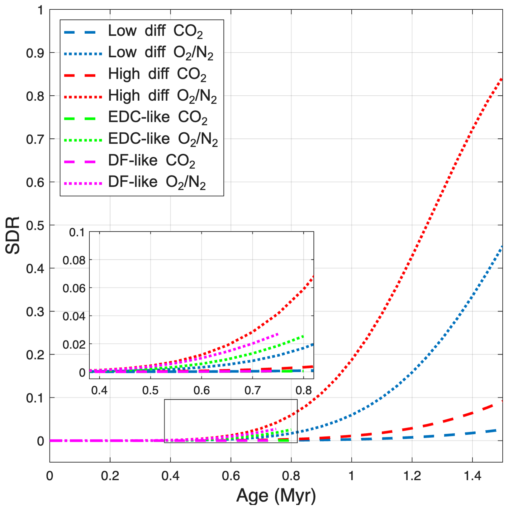
Figure 4 SDR for CO₂ (dashed) and the O₂ $/$ N₂ ratio (dotted) modeled with EPICA Dome C forcings (green), Dome F forcings (magenta), a low diffusion scenario (blue), and a high diffusion scenario (red). The inset shows each case between 0.4 and 0.8 Ma.

Table 1 Forcing values used to model each scenario to assess how reliable estimates of diffusive smoothing from existing ice core gas concentration measurements are. EDC surface temperatures approximate a glacial-cycle average. The SDR from 0 to 1.5 Ma of each scenario is shown in Fig. 4.

3.2 SDR sensitivity to input parameters

Here, we investigate the sensitivity of gas diffusion to four input parameters to the models: accumulation rate, ice thickness, surface temperature, and GHF. We hold three parameters constant and vary the fourth to gain an intuition for how SDR responds to each forcing parameter separately. Parameter values are chosen to keep the melt rate at zero. This ensures that the oldest ages are represented in this analysis and not destroyed by basal melt. The parameter values also are different between the CO₂ and the O₂ $/$ N₂ ratio model runs. We consider separate sets of parameters for CO₂ and O₂ $/$ N₂ because of the large difference in the diffusion rates of CO₂ and the O₂ $/$ N₂ ratio. Fixed parameter values for each gas are shown in Table 2. The range for each variable parameter is based on the physical properties of the study area. The effects of the parameters are interrelated. For example, the effect of varying accumulation depends on the assumed temperature, ice sheet thickness, and GHF. So, this analysis should be considered qualitative. Figures 5 and 6 show CO₂ and the O₂ $/$ N₂ ratio SDR sensitivity to input parameters.

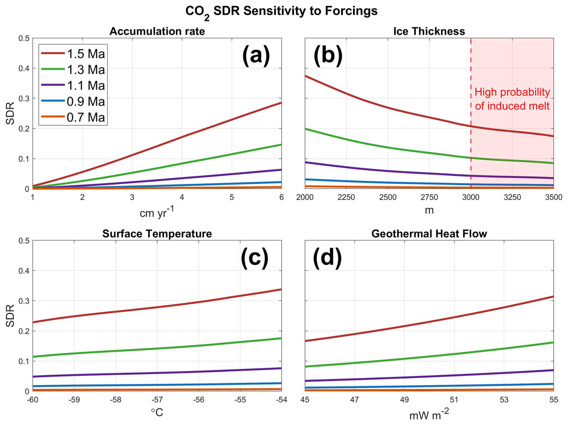
Figure 5 Sensitivity of CO₂ SDR to (a) accumulation rate, (b) ice thickness, (c) surface temperature, and (d) GHF. Parameter values are chosen to keep the melt rate at zero.

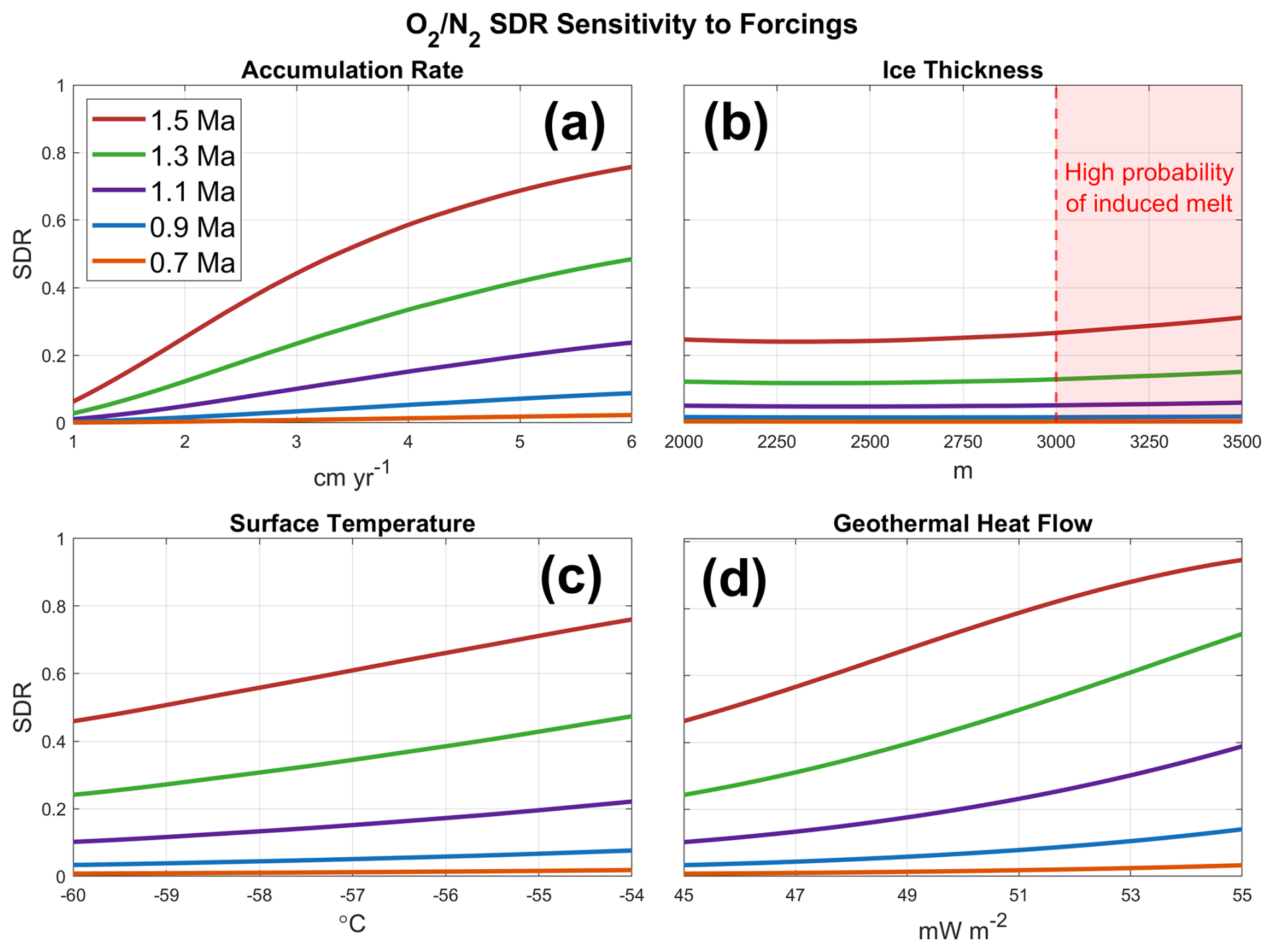
Figure 6 Sensitivity of O₂ $/$ N₂ ratio SDR to (a) accumulation rate, (b) ice thickness, (c) surface temperature, and (d) GHF. Parameter values are chosen to keep the melt rate at zero.

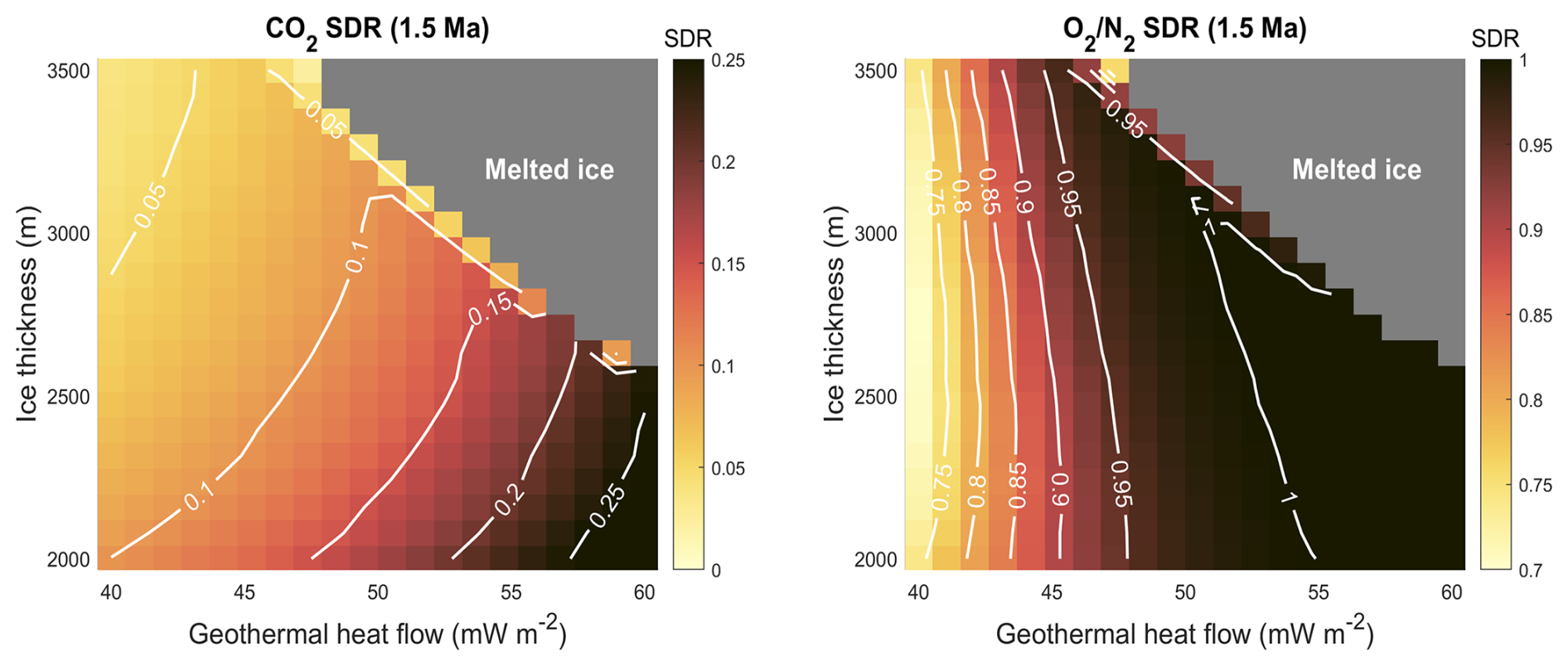
Figure 7 SDR in 1.5 Ma ice for CO₂ (left panel) and the O₂ $/$ N₂ ratio (right panel) with varying GHF and ice thickness. Note the different color scales. Accumulation rate is fixed at 3 cm yr⁻¹; surface temperature is fixed at −60 °C.

Table 2 Fixed parameter values for sensitivity analysis. We use different parameter values for each gas due to their different levels of diffusive smoothing. Values are set to maintain zero melt rate.

The SDR of CO₂ increases roughly linearly with accumulation rate, surface temperature, and GHF, and decreases with ice thickness. Increasing accumulation yields increased SDR (Fig. 5a). Higher accumulation enhances signal smoothing because the thinner layers near the bed cause steeper gas concentration gradients. The steep gradients increase diffusion more than the decrease in ice temperature from greater vertical advection of cold surface temperatures. Additionally, the relatively steep slope in Fig. 5a shows that accumulation rate has the largest impact on CO₂ signal preservation. The effect of surface temperature and GHF are simpler. Lower values reduce SDR because of colder temperatures and the changes are near linear for both (Fig. 5c and d). The response to ice thickness is more complex. Thicker ice columns result in lower SDR due to thicker layers and shallower gas concentration gradients. However, ice columns larger than ∼3000 m have a greater likelihood of basal melting, potentially removing old ice. Therefore, the sensitivity in Fig. 5b should not be interpreted to suggest maximizing ice thickness will minimize SDR. We explore scenarios with basal melt in more detail in Fig. 7.

The O₂ $/$ N₂ ratio model runs show similar results to those for CO₂. Accumulation rate's impact on gas concentration gradients dominates the impact from colder temperatures (Fig. 6a), and its relatively steep slope also shows its importance among the forcings. The O₂ $/$ N₂ ratio SDR is mildly more sensitive to GHF, due to higher sensitivity of O₂ permeability to temperature compared to CO₂. Similarly to CO₂, minimizing surface temperature and GHF will minimize SDR for the O₂ $/$ N₂ ratio, too (Fig. 6c and d). Unlike CO₂, ice thickness has a relatively weak effect on the O₂ $/$ N₂ ratio SDR. In thicker ice columns, we find the impact on temperature slightly dominates the impact on gas concentration gradients as demonstrated by the slightly positive slope in Fig. 6b. This arises from a higher sensitivity to temperature in the permeability of O₂ compared to CO₂. However, in shallower ice columns, where temperatures are cooler compared to thicker ice columns, the relatively flat slope implies the impacts on temperature and layer thinning are about equal and opposite. The lower dissociation pressure of O₂ compared to CO₂ causes more diffusion in the warmer temperatures of thick ice columns. Ice thickness's weak effect on the O₂ $/$ N₂ ratio SDR is further highlighted in Fig. 7.

Basal melt is important to consider for SDR and site selection. Under scenarios where basal melt rates are low, about 0.1 mm yr⁻¹, ice older than 1.5 Ma is removed but ice of 1.5 Ma age remains. The melting of the older ice, without removing the 1.5 Ma ice, creates additional vertical space for the 1.5 Ma ice to occupy, thus reducing the thinning. The reduced thinning of 1.5 Ma ice thus results in improving gas signal preservation. Figure 7 shows SDR values for CO₂ and the O₂ $/$ N₂ ratio in 1.5 Ma ice under varying GHF and ice thickness, with fixed accumulation rates of 3 cm yr⁻¹ and surface temperatures of −60 °C. The signal preservation enhancing effect of low melt rates is apparent at the boundary between preserved 1.5 Ma ice and melted ice, where SDR values are lower by about 5 % (Fig. 7). This is most important for CO₂ signal preservation, as we see that the O₂ $/$ N₂ signals are almost fully damped above 45 m W m⁻². However, producing such a low melt rate requires a specific range of forcing values in this simplified model, so a site with these conditions is likely rare.

3.3 Atmospheric gas diffusion in the interior of the east Antarctic ice sheet

The gas diffusion model is now applied to the COLDEX study area (Fig. 8). We will first discuss the distribution of old ice in each of the three regions – the Saddle Region, the Deep Basin, and the Foothills – then discuss the CO₂ and the O₂ $/$ N₂ ratio SDRs. The accumulation rate and ice thickness inferred from the airborne radar data (Young et al., 2025a) is shown in Fig. 8a and b and the surface temperature forcing in Fig. 8c. Estimates of GHF (Stål et al., 2020; Shen et al., 2020; An et al., 2015; Maule et al., 2005; Martos et al., 2017; Shapiro and Ritzwoller, 2004; Purucker et al., 2013; Hazzard and Richards, 2024) show considerable variability and their relative accuracy cannot be assessed; therefore, we use uniform GHF values of 45, 50, and 55 m W m⁻². We consider the near-basal ice age as the age of ice that is 2 % of the ice column's thickness above the bed (Fig. 8g–i), which is between 40 and 80 m above the bed in the COLDEX study area. We use the 2 % threshold to facilitate comparison among the study area.

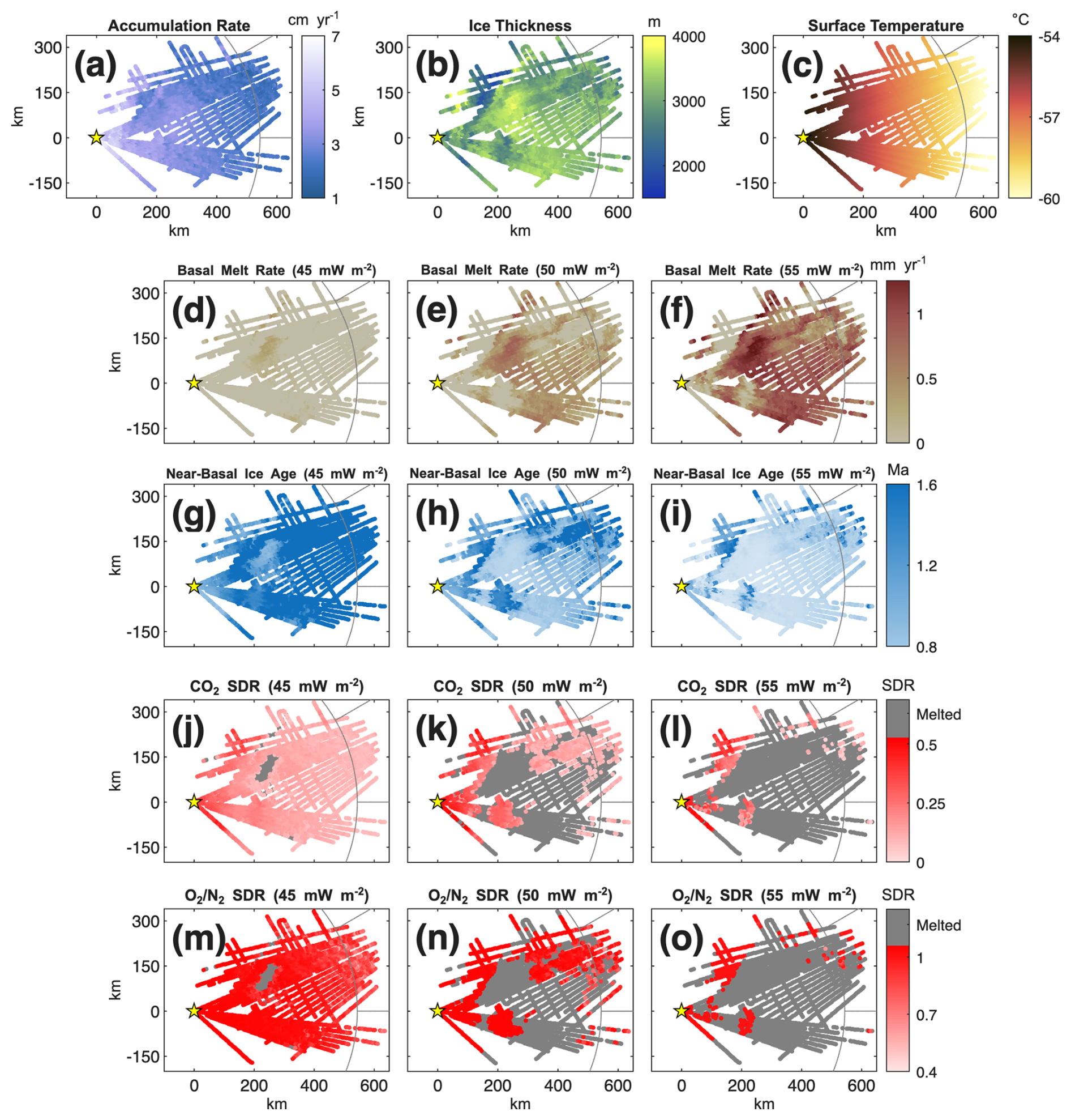
Figure 8 (a) Accumulation rate and (b) ice thickness were measured or inferred with aerial radar, provided by COLDEX. (c) Surface temperature is interpolated over the region based on the Easting from the South Pole. Each model output is calculated under three GHF scenarios: 45, 50, and 55 m W m⁻². (d, e) Basal melt rate and (g–i) the age of near-basal ice (2 % of ice thickness above the bed, ∼20–40 m) as calculated by the 1D, steady-state ice and heat flow model. (j–l) SDR for CO₂ in 1.5 Ma ice; grey points indicate where 1.5 Ma ice is melted. (m–o) SDR for the O₂ $/$ N₂ ratio in 1.5 Ma. The yellow star represents the South Pole.

The Saddle Region and the Foothills retain old ice, while the Deep Basin has mostly lost the oldest ice to basal melt (Fig. 8g–i). Only in the low GHF scenario does the Deep Basin retain old ice. Figure 8d–f shows how each GHF scenario increases the basal melt, particularly in the Deep Basin. It is also important to note that the Saddle Region is downstream from the Deep Basin and advection is not considered in our model; we discuss the effects of advection in Sect. 4.1. The Foothills contain the oldest ice under all GHF scenarios, but the calculated age is variable due to the considerable variability in ice thickness in the region.

We discuss SDR in terms of its value at 1.5 Ma. The lowest CO₂ SDR (Fig. 8j–l) is in the Foothills and in the Deep Basin when there is old ice present. CO₂ SDR tends to be higher in the Saddle Region where accumulation rates are higher, consistent with the results in Sect. 3.2. The variable ice thickness in the Foothills contributes to variability in CO₂ SDR but is not as significant as the variability in ice age. For each GHF scenario, the CO₂ SDR varies marginally in the Foothills (∼3 %–10 %) and varies more significantly in the Saddle Region (∼18 %–30 %).

The O₂ $/$ N₂ ratio SDR (Fig. 8m–o) follows a similar pattern to the CO₂ SDR. The lowest O₂ $/$ N₂ ratio SDR is in the Foothills, although it is still much higher than the SDR for CO₂. Both the Deep Basin and Saddle Region have nearly 100 % SDR. In the Deep Basin, this is because of the warm temperatures in the deep ice while in the Saddle Region it is because of the high accumulation rate and steep gas concentration gradients in the basal ice. The Foothills is the only region with SDR significantly below 1, due to the effects of low melt rates as described in Sect. 3.2. Although, there is considerable variability in the SDR in the Foothills.

Uncertainties in GHF have a larger effect on the distribution of old ice compared to the diffusion of gas signals. In the Deep Basin, where ice thickness is consistently around or above 3000 m, we see the amount of old ice present changes dramatically with different GHF values. At 45 m W m⁻², old ice is abundant in the basin, only absent where ice thickness nears 4000 m. However, at 50 m W m⁻² most of the old ice is gone except towards grid-south, and at 55 m W m⁻² there is virtually no old ice in the basin. Assuming uniform GHF, the oldest ice will be located near either the South Pole, the Foothills, or both according to the model, with the Foothills having better conditions for atmospheric gas signal preservation. Additionally, advection will affect the presence of old ice in the Saddle Region, as discussed in Sect. 4.1.

4 Discussion

4.1 Impact of advection

We have presented 1D results and have not assessed the impact of advection. Advection will be important to consider because even the slow horizontal velocities in the region, 1–2 m yr⁻¹ in the survey region, imply that 1.5 Ma ice has travelled hundreds of kilometers. Unfortunately, modeling SDR for the full study area with flowline models is intractable both because of the computational time and the increasing number of assumptions needed to force the model. We note that the gas diffusion model can be applied to any ice thinning and temperature scenario and thus is compatible with output from ice flow models as long as this information is tracked (e.g. Chung et al., 2023; Parrenin et al., 2025). Consideration of specific ice core sites should employ flow band models where parameter ranges for the upstream area can be carefully considered.

The 1D model results are best for gaining qualitative information about the broader regions which are likely to best preserve atmospheric gas records. The primary limitation is that small scale variations in forcing parameters, such as bedrock topography, can produce results that appear favorable but where advection would have instead significantly imprinted the conditions from upstream on the ice at that location. Thus, considering the conditions in the upstream direction is useful for interpreting the results at any individual location. For example, in our results the model signifies the presence of old ice in the Saddle region (Fig. 8g–i). However, ice flows from the Foothills, through the Deep Basin, where old ice likely melts away, before reaching the Saddle Region. Thus, the Saddle Region is less likely to preserve old ice than the 1D model results may suggest.

4.2 Implications for ice core site selection

The most favorable site conditions for the preservation of gas signals in a deep ice core are where accumulation rates, basal melt rates, and surface temperatures are low, and ice thickness is moderate, between ∼2500 and ∼3000 m. If a location with low GHF can be identified, then greater ice thicknesses are preferred because basal melt is avoided and the gas concentration gradients are smaller, reducing the amount of diffusion.

The Deep Basin, due to its large ice thickness, results in too much basal melt, removing the old ice. Even in the low GHF scenario (45 m W m⁻²), some of this region experiences basal melt (Fig. 8d). We note that if the GHF is unusually low, the Deep Basin could provide exceptional preservation conditions; however, geophysical observations supporting such a unique combination would be necessary to justify further exploration in this region. In the Saddle Region, accumulation rates are relatively high (∼6 cm yr⁻¹), steepening gas concentration gradients in the basal ice and increasing signal diffusion. The SDR is higher in the Saddle Region than in the Foothills, as seen in Fig. 9. We also note that the ice has flowed across the Deep Basin, so if melt has removed the old ice in the Deep Basin, it would not be present in the Saddle Region. Thus, both the Deep Basin and the Saddle Region are not optimal locations for a deep ice core. While there remains the possibility of finding an ice core site in these regions, it would likely require an unusually low GHF in the Deep Basin (e.g. Hazzard and Richards, 2024) so that ice is not removed there.

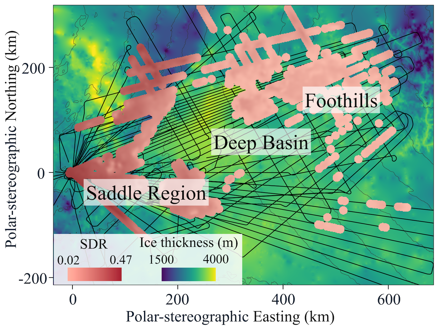
Figure 9 CO₂ SDR in 1.5 Ma ice under 50 m W m⁻² GHF (Fig. 8k) and ice thickness and elevation (Fig. 2a).

The lower accumulation rates and moderate ice thickness make the Foothills a more promising region for a deep ice core. Old ice is more common and SDRs are lowest in this region. Within the Foothills, the grid-south portion of the foothills have thicker ice columns than the grid-north portion, increasing melt rates and decreasing the old ice present. This leaves the grid-north foothills as the most promising location (Fig. 9). Even though this is the most promising region, the presence of 1.5 Ma ice is variable and should be evaluated at a particular site to ensure its presence. Sites where the melt rate might be low enough, but non-zero, to decrease SDR as described in Sect. 3.2 should not be sought, since the narrow range of necessary forcings, the uncertainties associated with the model, and the impact of advection make looking for such a site impractical.

Our results show that CO₂ SDR for 1.5 Ma ice does not exceed 13 % in the grid-north Foothills and averages 5 % given 50 m W m⁻² GHF (Fig. 8k). However, the SDR for the O₂ $/$ N₂ ratio in the grid-north Foothills is still high, with a mean value of 89 % (Fig. 8l). There is uncertainty associated with the fraction of gas signal lost to diffusion in the model arising from uncertain gas parameter values (see Sect. 4.4). Nonetheless, we still expect that CO₂ signals will experience only a small amount of diffusion, while the O₂ $/$ N₂ ratio will experience significantly more. The difference between the SDR for CO₂ and the O₂ $/$ N₂ ratio is partly due to the different frequency in the climate record; the SDR for a 20 kyr CO₂ signal is 28 % for a typical site in the Foothills whereas the 40 kyr SDR is 8 %. Therefore, even though old ice is likely present in the grid-north Foothills and CO₂ may be well preserved, the damping of precession signals in the O₂ $/$ N₂ ratio from this region may preclude dating of the ice core. Measurements of total air content (TAC) may provide another method for dating an old ice core (e.g. Raynaud et al., 2007), but this method comes with its own complications (Vudayagiri et al., 2025) as climate and elevation changes can overprint the insolation signal. Future work could consider how TAC signals may diffuse in old ice. For 1.2 Ma ice (when the MPT is thought to have begun; Clark et al., 2006) the SDR for the O₂ $/$ N₂ ratio is lower than at 1.5 Ma (∼0.5–0.7 in the grid-north Foothills), so it may be possible to track precession cycles through the MPT.

4.3 Potential impacts of basal ice units

The 1D model we use assumes a continuous depth-age relation to the bed; however, radar imaging shows that stratigraphic layering is lost hundreds of meters above the bed and finds diffuse scattering in portions of the deep ice (Young et al., 2025a). Work around Dome C suggests there may be basal layers of stagnant ice (Lilien et al., 2021; Chung et al., 2023; 2024), which can affect the inferred depth-age relationship. Analysis of the radar data at ice core locations (Mutter and Holschuh, 2025) show that the continuous climate record can be preserved at depths with diffuse scattering. We assume that the climate record is undisturbed to the bed in this study. However, if instead the basal unit is mechanically decoupled (e.g. Lilien et al., 2021; Chung et al., 2023), then the thickness of the deforming ice column is less than the total ice thickness. This would result in greater layer thinning as well as colder temperatures because the old ice is higher in the ice column.

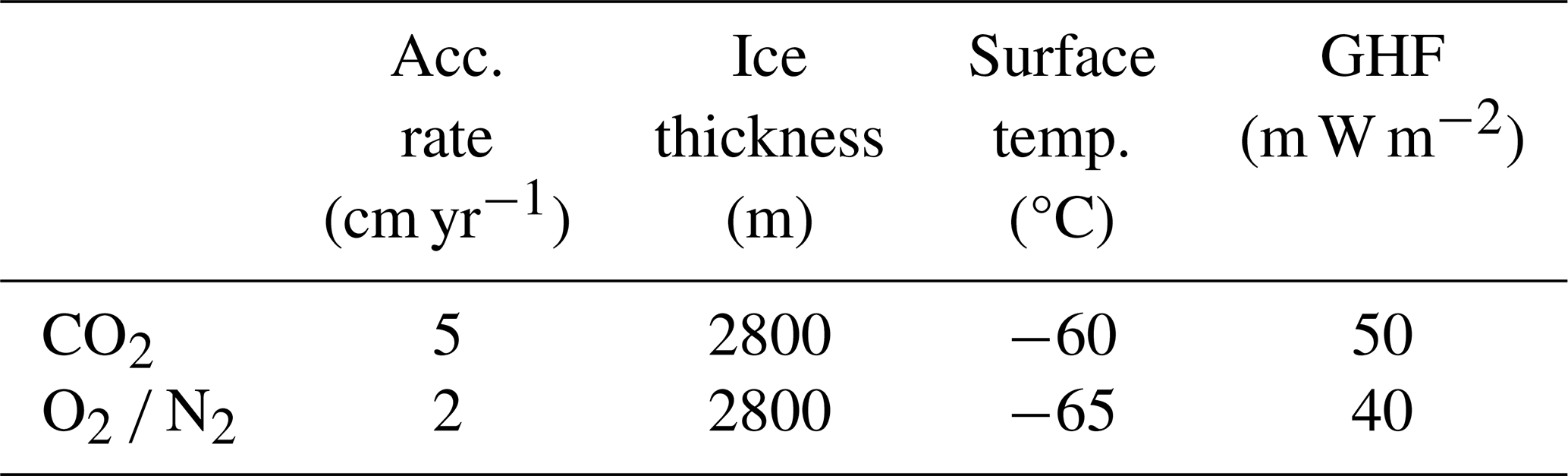
To assess the impact of a potential basal ice layer, we perform three model runs and compare their SDRs. Case 1 is the control with 2700 m ice thickness, 50 m W m⁻² GHF, 2 cm yr⁻¹ accumulation rate, and −60 °C surface temperature. Case 2 investigates the impact of a change in layer thickness while keeping the temperature the same. Case 3 investigates the impact of a change in temperature while keeping the layer thickness the same.

The temperature and age profiles of the three cases are shown in Fig. 10. We do not directly incorporate a non-deforming basal layer and instead adjust the GHF to simulate its impacts. Case 2 simulates a 10 % (270 m) basal ice layer to assess the impact of layer thinning from a non-deforming basal ice layer; we model a thinner ice column (2430 m) but match the Case 1 temperature. Case 3 simulates a 3000 m ice column with the bottom 10 % (300 m) non-deforming to assess the impact of a change in ice temperature from a basal ice layer; we model the same thickness (2700 m, so the depth-age profile is the same), but match the temperature profile to a model run of Case 1 extended to 3000 m ice thickness (Case 1^* in Fig. 10) by reducing the GHF. The cases and resulting SDR are summarized in Table 3.

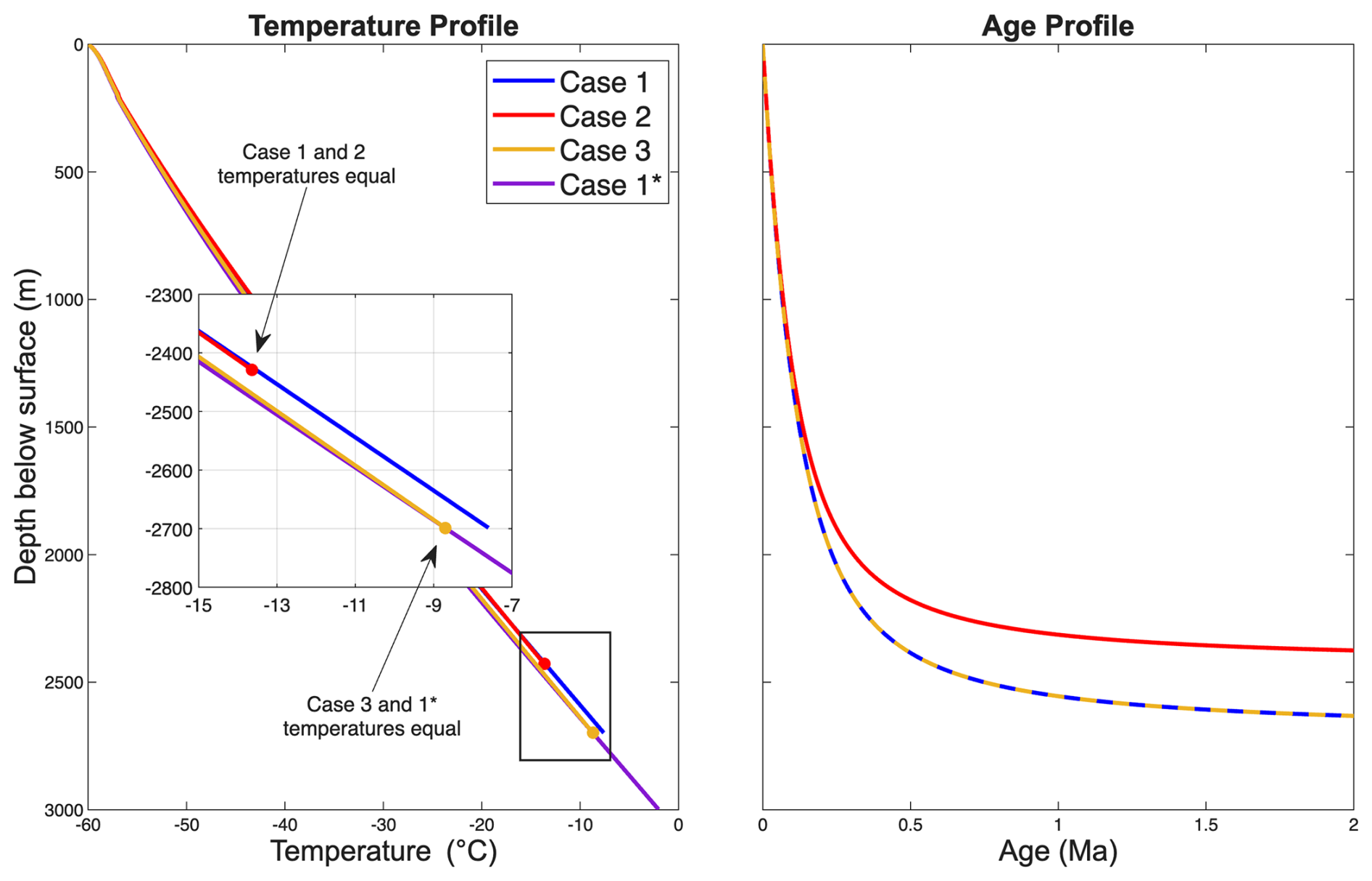
Figure 10 The temperature (left panel) and age (right panel) profiles for each model case. The age profiles of Cases 1 and 3 are the same. Note that depth is measured from the surface, not as height above the bed.

Table 3 Deforming ice thickness, basal ice layer thickness, total ice thickness, GHF, and SDR at 1.5 Ma for each basal ice layer case. Case 1 is a control which simulates a 2700 m deforming ice column. Case 2 simulates the presence of a 270 m basal ice layer to assess the impact of increased layer thinning from a basal ice layer. Case 3 simulates the presence of a 300 m basal ice layer to assess the impact of decreased temperature from a basal ice layer. Each case uses an accumulation rate of 2 cm yr⁻¹ and a surface temperature of −60 °C.

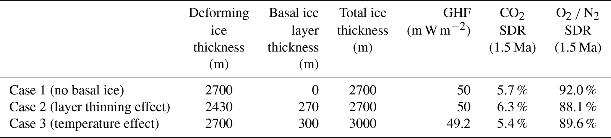
In Case 2, a thinner deforming ice column increases CO₂ SDR and decreases the O₂ $/$ N₂ ratio SDR. This aligns with what we would expect given the parameter sensitivity analysis in Sect. 3.2 (see Figs. 5b and b). In Case 3, a lower ice temperature from the presence of a basal ice layer decreases the CO₂ and the O₂ $/$ N₂ ratio SDRs. This also aligns with our expectations since the presence of a basal ice layer decreases the ice temperature, reducing diffusion. The difference in SDR for all cases is small, so we do not expect the presence of a basal ice layer to dramatically alter the preservation of gas signals. In each case, CO₂ remains well preserved and the O₂ $/$ N₂ ratio is poorly preserved.

4.4 Uncertainties from gas parameters

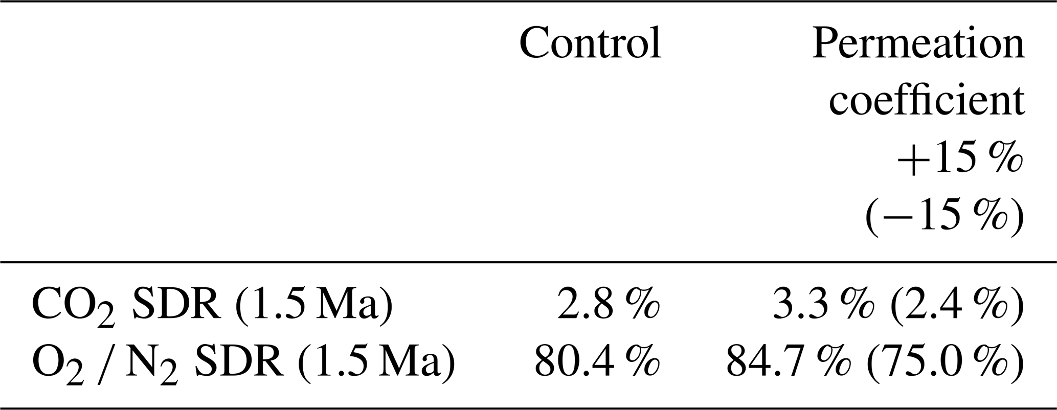
We perform sensitivity studies to assess the possible implications of the uncertainty in gas permeation parameters for our result. All sensitivity runs use forcing values identical to those in Fig. 3 (2 cm yr⁻¹ accumulation rate, 3000 m ice thickness, 50 m W m⁻² GHF, −60 °C surface temperature). Salamatin et al. (2001) report a ±15 % uncertainty for the permeation coefficient of O₂, so we conduct simulations using permeation coefficients that span this range. Ahn et al. (2008) do not provide an uncertainty for the permeability of CO₂ so we apply the same 15 % uncertainty range. Oyabu et al. (2021) have previously demonstrated that O₂ permeation values an order of magnitude faster than those we consider here yield unrealistically high smoothing compared to O₂ $/$ N₂ measurements from the Dome Fuji core. Those researchers also show that the permeation coefficients of Salamatin et al. (2001) yield diffusive smoothing in reasonable agreement with the Dome Fuji measurements, increasing confidence in our parameterizations. However, the permeation values provided by Salamatin et al. (2001) (the “slow set”) are tested over a limited temperature range, and the values given by Ikeda-Fukazawa et al. (2004) (the “fast set”) approach the values in the “slow set” at higher temperatures, like those near the bed of the ice sheet. Thus, our use of the “slow set” in this study may provide a more conservative estimation of diffusive smoothing of O₂ $/$ N₂. Future ice core measurements may improve our understanding of the temperature dependence of these permeation coefficients. Table 4 shows the SDR for each gas from each model run. Uncertainty in the permeation coefficient of CO₂ affects the SDR by <1 %. Uncertainty in the permeation coefficient of O₂ can change the O₂ $/$ N₂ ratio SDR by about ±5 %. The study area will be affected by this uncertainty equally, and so the pattern of where SDR is low will not be altered significantly by these results. The expected SDR we find in this study is much more dependent on ice sheet physical properties than the uncertainty in gas permeation.

Table 4 CO₂ and O₂ $/$ N₂ ratio SDR based on permeation coefficient uncertainties. Uncertainty ranges are based on the uncertainty of the permeation coefficient of O₂ (Salamatin et al., 2001). All model runs are done with the input forcings shown in Fig. 3. “Control” refers to the model run with no alterations to gas parameter values.

5 Conclusions

Gas signal preservation in a 1.5 Ma ice core from the COLDEX study area between South Pole and Dome A was investigated using gas diffusion models. We expand on the work of Bereiter et al. (2014) who showed that CO₂ variations, but not the O₂ $/$ N₂ ratio, are likely preserved at an idealized location similar to the Little Dome C site that the Beyond EPICA Oldest Ice program has recently completed drilling. We find that the conditions most likely to preserve atmospheric gas signals are a low accumulation rate, minimal surface temperature, minimal GHF, and moderate ice thickness between 2500 and 3000 m. We identify the Foothills region, the portion of the study area closest to Dome A, as more likely to preserve atmospheric gas records. CO₂ signals (with a period of 40 kyr) do not lose more than 13 % of their amplitude in the Foothills compared to up to 43 % elsewhere in the study area. The Foothills also better preserve the O₂ $/$ N₂ ratio; however, O₂ $/$ N₂ signal preservation is poor with 89 % signal loss on average in the Foothills. The grid north portion of the Foothills has more moderate ice thickness and is less likely than the grid south portion to lose old ice to basal melt.

Our analysis focused on four boundary conditions. The accumulation rate is the dominant factor for diffusion: high accumulation rates lead to more layer thinning in old ice, resulting in an increased gas concentration gradient and thus more diffusion. This outweighs any reduction in diffusion from colder temperatures in the ice column. Thicker ice has a similar effect to low accumulation rates by reducing layer thinning. For CO₂, this results in better gas preservation; the O₂ $/$ N₂ ratio is not as sensitive to this due to a greater effect from higher temperatures in thicker ice columns. However, thicker ice also promotes basal melting and removal of 1.5 Ma ice. Thus, moderate ice thickness of 2500 to 3000 m is better with the important caveat that thicker ice is better for CO₂ preservation if the GHF is low enough to not induce substantial basal melt.

GHF is the least constrained parameter, introducing large uncertainty in whether 1.5 Ma ice will be preserved. Atmospheric gas preservation also has uncertainty due to unknown gas parameter coefficients. We note that gas parameter coefficients will affect all areas of the study area similarly, so while the absolute preservation may be uncertain, the relative pattern of preservation should be consistent. The Foothills region, particularly to the grid north, is the most likely region to preserve atmospheric gas records reaching 1.5 Ma and should be explored in more detail to determine whether it is suitable for a deep ice core.

Our results suggest that the recovery of a continuous ice core record back to 1.5 Ma would not experience significant diffusive smoothing of CO₂ signals, under the recommended conditions. Thus, such an ice core will provide insights into the role CO₂ played in the MPT. However, dating such an ice core will likely require a method other than precession cycles apparent in the O₂ $/$ N₂ ratio. The O₂ $/$ N₂ ratio diffuses significantly in ice older than 1 Ma, but if high resolution measurements can distinguish precession cycles in a damped O₂ $/$ N₂ record, some dating may still be achievable.