Living on the edge: Response of Late Cretaceous rudist bivalves (Hippuritida) to hot and highly seasonal climate in the low-latitude Saiwan site, Oman

Earth's climate history serves as a natural laboratory for testing the effect of warm climates on the biosphere. The Cretaceous period featured a prolonged greenhouse climate characterized by higher-than-modern atmospheric CO₂ concentrations and mostly ice-free poles. In such a climate, shallow seas in low latitudes probably became very hot, especially during the summers. At the same time, life seems to have thrived there in reef-like ecosystems built by rudists, an extinct group of bivalve molluscs. To test the seasonal temperature variability in this greenhouse period, and whether temperature extremes exceed the maximum tolerable temperatures of modern marine molluscs, we discuss a detailed sclerochronological (incrementally sampled) dataset of seasonal scale variability in shell chemistry from fossil rudist (Torreites sanchezi and Vaccinites vesiculosus) and oyster (Oscillopha figari) shells from the late Campanian (75-million-year-old) low latitude (3° S paleolatitude) Saiwan site in present-day Oman. We combine trace element data and microscopy to screen fossil shells for diagenesis, before sampling well-preserved sections of a Torreites sanchezi rudist specimen for clumped isotope analysis. Based on this specimen alone, we identify a strong seasonal variability in temperature of 19.2 ± 3.8 to 44.2 ± 4.0 °C in the seawater at the Saiwan site. The oxygen isotopic composition of the seawater (δ¹⁸O_sw) varied from −4.62 ± 0.86 ‰ VSMOW in winter to +0.86 ± 1.6 ‰ VSMOW in summer.

We use this information in combination with age modelling to infer temperature seasonality from incrementally sampled oxygen isotope profiles sourced from the literature, sampling multiple shells and species in the assemblage. We find that, on average, the Saiwan seawater experienced strong seasonal fluctuations in monthly temperature (18.7 ± 3.8 to 42.6 ± 4.0 °C seasonal range) and water isotopic composition (−4.33 ± 0.86 to 0.59 ± 1.03 ‰ VSMOW). The latter would strongly bias the interpretation of stable oxygen isotopes in shell carbonate without independent control on either temperature or seawater composition.

Combining our seasonal temperature estimates with shell chronologies based on seasonal cyclicity in stable isotope records and daily variability in trace element data, we show that T. sanchezi rudists record temperatures during the hottest periods of the year as well as during the winters, which were characterized by cooler temperatures and enhanced influx of freshwater. Both O. figari and V. vesiculosus plausibly stopped growing during these seasonal extremes. This study aims to demonstrate how high-resolution geochemical records through fossil mollusc shells can shed light on the variability in past warm ecosystems and open the discussion about the limits of life in the shallow marine realm during greenhouse climates. Future work should apply the clumped isotope paleothermometer on incrementally sampled bio-archives to explore the upper-temperature limits experienced by calcifiers in different environments throughout geological history.

1 Introduction

Ongoing anthropogenic global changes, including greenhouse gas emissions and land use changes, are projected to increase global mean annual temperatures by multiple degrees with respect to pre-industrial conditions, while at the same time causing severe biodiversity loss (IPCC, 2023; World Wildlife Fund, 2021). These crises are intricately linked, but assessing the effect of climate change on biodiversity loss requires information on the response of biodiversity to climate extremes under various (paleo)climate scenarios. The geological record provides a rich source of such information in the form of fossil bio-archives that record climate and environmental change on the scale of days to decades, while testifying to biodiversity by their presence in the rock record (Huyghe et al., 2012; Ivany, 2012; Schmitt et al., 2022). Past ecosystems thus serve as natural experiments for testing the limits of life during periods of global change or in exceptionally warm periods (Cermeño et al., 2022; Jones et al., 2022; de Winter et al., 2017b).

Examples of hot periods that may reveal ecosystems' functioning under high-temperature climate scenarios include the early Triassic super greenhouse (Sun et al., 2012), the Mid-Cretaceous Climate Optimum (Jones et al., 2022) or the Eocene hothouse period (Evans et al., 2013; de Winter et al., 2020b). Milder, yet still warmer than present-day, scenarios of interest include the Late Cretaceous (O'Hora et al., 2022; Petersen et al., 2016a; de Winter et al., 2020a), the Miocene Climatic Optimum (Batenburg et al., 2011; Harzhauser et al., 2011) and the Pliocene Warm Period (Dowsett et al., 2013; Wichern et al., 2023; de Winter et al., 2024). While these periods feature long-term, equilibrated climate states instead of fast, transient climate change events (like modern anthropogenic warming), they can yield useful insights into the long-term response of the climate system and biosphere to prolonged radiative forcing (Burke et al., 2018). For example, some of these past environments, most notably shallow marine ecosystems, are thought to have reached temperatures exceeding the temperature range of modern equivalent ecosystems (de Winter et al., 2020a; Huang et al., 2017; Jones et al., 2022). These temperatures probably exceeded the maximum temperature tolerance at which modern shallow marine species can complete their life cycle, which is typically estimated in the order of 38–42 °C (Compton et al., 2007; Huang et al., 2017; Jones et al., 2022; de Winter et al., 2020a). Conditions that exceed this threshold (> 38 °C) are considered high-temperature conditions for shallow marine calcifiers to live in.

A striking conundrum arises in the Late Cretaceous Tethys Ocean margins, which were inhabited by large rudist bivalves biostromes (Skelton, 2018) despite apparently high water temperatures. The atmospheric CO₂ concentrations during the Campanian (83.6–72.1 Ma; Gradstein et al., 2020) were ∼ 600 ppmv (roughly 2 × pre-industrial concentrations; Wang et al., 2014), resulting in low- to mid-latitude mean annual sea surface temperatures (SST) of 20–25 °C (O'Brien et al., 2017), roughly 5–10 °C warmer than the current global mean annual temperature. In low-latitude Tethyan margins, mean annual temperatures likely exceeded 30 °C (Steuber et al., 2005), with summer temperatures estimated above 40 °C in some localities (Steuber, 1999; de Winter et al., 2017b, 2020a). A big caveat of these estimates is that they rely on the temperature dependence of stable oxygen isotope analyses and are contingent on assumptions of (seasonally) constant stable oxygen isotope composition of Tethyan seawater, which is known to have fluctuated over time (Price et al., 2020; Walliser and Schöne, 2020). If correct, such temperatures exceed the temperature threshold of 38 °C mentioned above and are at or above the lethal thermal limits for modern marine invertebrates (typically 42–50 °C; Clarke, 2014; Compton et al., 2007). These temperatures approach the thermal threshold above which critical macromolecules such as ATP, proteins, and enzymes used by non-extremophile organisms denature (> 50 °C) (Clarke, 2014; Tehei et al., 2005; Tehei and Zaccai, 2007), hampering key metabolic functions. Yet, despite these apparent temperature extremes, abundant and diverse fossil shallow marine ecosystems suggest that rudists thrived in these environments (Gili and Götz, 2018; Ross and Skelton, 1993). This raises the question of whether these paleotemperature reconstructions are accurate, and if so, whether these ancient molluscs were somehow adapted to grow their shells at these extreme temperatures.

In an attempt to resolve this thermal tolerance conundrum, we investigate the growth and chemical composition of two species of rudist bivalve (Torreites sanchezi and Vaccinites vesiculosis) and one oyster species (Oscillopha figari) from the low-latitude Tethyan site in the Saiwan area in east-central Oman (Kennedy et al., 2000; Schumann, 1995). Our analysis combines new sclerochemical data, including clumped isotope analyses, with existing stable oxygen isotope datasets from the literature. We aim to test how the growth of these animals responds to seasonal temperature extremes. To obtain accurate seasonal temperature reconstructions that are independent of the Tethyan seawater composition and ex vivo diagenetic alteration, we combine information on trace elements, stable oxygen isotopes, and clumped isotopes. Using a new clumped isotope dataset, we first demonstrate that T. sanchezi records temperatures in their shells that significantly exceed the threshold at which modern marine molluscs thrive. We then build on our clumped isotope dataset to test how shell growth was influenced by these seasonal temperature extremes in this paleoenvironment by combining our results with stable oxygen isotope records from the literature, augmented with new shell chronologies and growth models. We contrast our seasonality and growth rate reconstructions with data on the thermal ranges of modern bivalves to compare the tolerance of biostrome-building rudists in the Late Cretaceous with modern species. Ultimately, this case study will open the discussion of the ability of marine life to adapt to hot climates and provide lessons for the interaction between climate change and marine biodiversity.

2 Materials and Methods

2.1 Fossil mollusc specimens

The mollusc shells utilized in this work originate from the Samhan Formation in the Saiwan area of Oman in the Huqf desert (20°39^′ N, 57°31^′ E; see Fig. 1A). The biostromes in this locality were dated as late Campanian (∼ 75 Ma) based on ammonite biostratigraphy by Kennedy et al. (2000). The paleolatitude of the site at 75 Ma was 3° S according to reconstructions following http://paleolatitude.org (last access: 12 November 2025; van Hinsbergen et al., 2015) based on the paleomagnetic reference frame by Vaes et al. (2023). The locality was described by Schumann (1995) as exposing Vaccinites-dominated rudist biostromes in which rudist bivalves are preserved in their life position (see also Fig. 1B–C). The V. vesiculosus and T. sanchezi specimens used and reused in this study originate from Unit IV in profile 1 of Schumann (1995), which is equivalent to unit 2 in Philip and Platel (1995). The thick-shelled O. figari oysters were collected in the marly layer just above the biostrome (see also Fig. 1B–C and de Winter et al., 2017b).

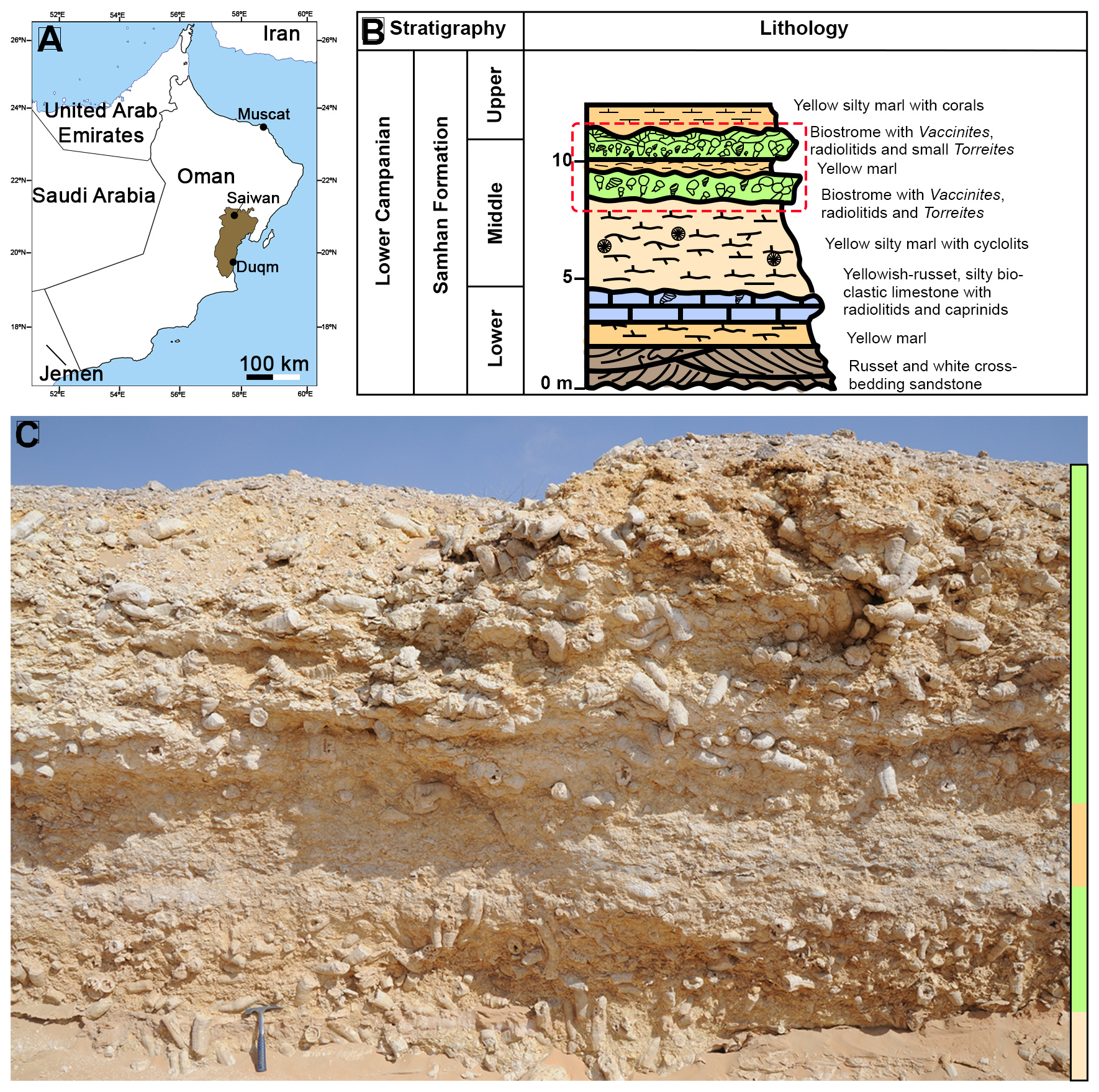
Figure 1 (A) Map of the geographical location of the Late Campanian Samhan Formation in the Saiwan area in the central part of the Sultanate of Oman. (B) Lithostratigraphic column showing the stratigraphic context of the characteristic members of the Samhan Formation. The red dashed box indicates the stratigraphic location of the outcrop pictured in panel (C). The marly layer containing O. figari referred to in the text is the brown layer in between the two green members in the dashed red box. (C) Outcrop showing the two Vaccinites-dominated biostromes, the lower of which contained the T. sanchezi and V. vesiculosus specimens investigated in this study (indicated by the schematic images of the species). The O. figari specimen was collected in the marly layer just above the biostrome containing the other specimens (indicated by the schematic image), between the two green units in panel (B). Panel (B) was modified after Philip and Platel (1995).

Table 1 Overview of data used in this study and their sources.

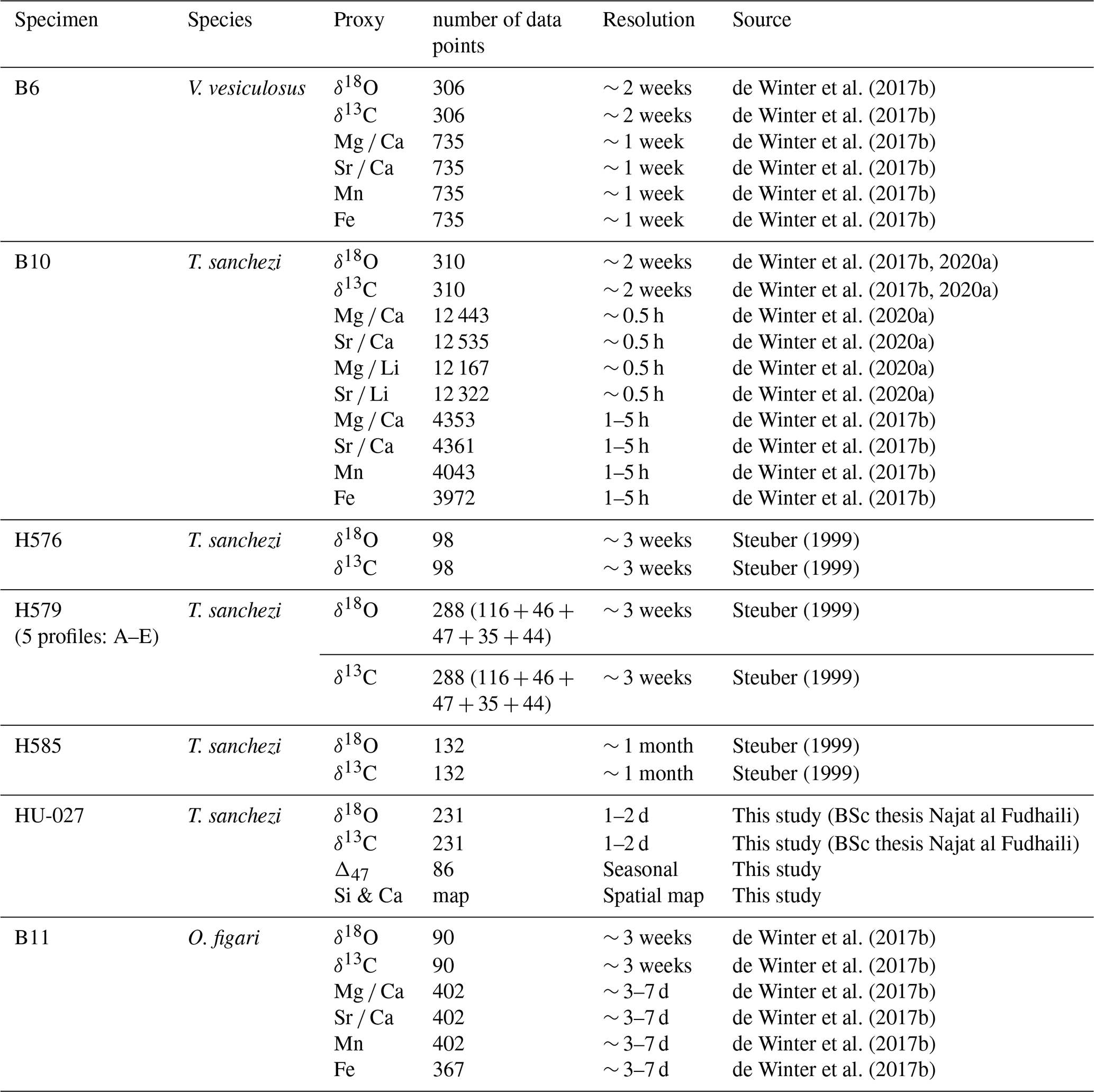
All specimens described in this study were sampled in longitudinal cross-sections through the axis of maximum growth using a combination of hand drilling and computer-assisted microdrilling using slow-rotating tungsten carbide dental drills. Table 1 gives an overview of the data used in this study, its temporal resolution and the source of datasets in cases where they have been reused from the literature. V. vesiculosus specimen “B6”, T. sanchezi specimen “B10” and O. figari specimen “B11” were described in de Winter et al. (2017b) and stable isotope (δ¹⁸O and δ¹³C) and trace element (Mg, Sr, Ca, Mn, Fe) data presented in that study are used here. Specimen B10 was also subject of a study by de Winter et al. (2020a), in which more detailed, daily scale trace element measurements (Mg $/$ Ca, Sr $/$ Ca, Mg $/$ Li and Sr $/$ Li) were presented and discussed. Stable isotope (δ¹⁸O and δ¹³C) data from T. sanchezi specimens “H576”, “H579” and “H585” was previously reported in Steuber (1999). Of these, specimen H579 was sampled in 5 parallel sections (“H579A-E”).

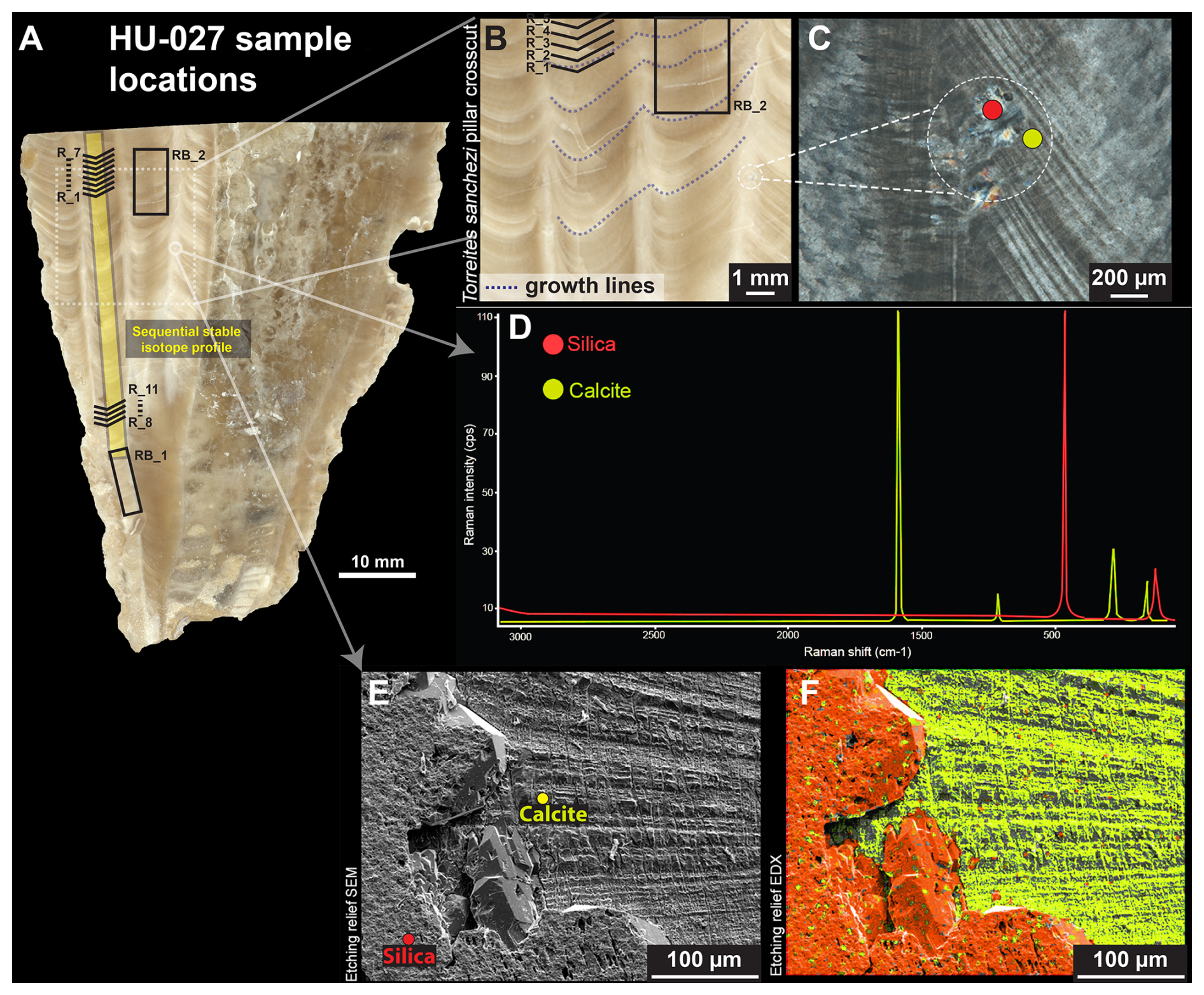
Figure 2 (A) High-resolution colour scan of a cross-section through T. sanchezi specimen HU-027 with the location of samples for δ¹⁸O, δ¹³C (yellow rectangle) and clumped isotope analysis (black text and lines). (B) Zoomed-in insert showing fine lamination in columns through HU-027, the location of samples RB_2 and R_1–R_5, and examples of isochronous growth lines (dashed lines) that link the timing of growth between pillars in the cross-section. (C) Cross-polarized light image of the edge of a shell column showing locations for characterizing diagenetic (silicified) and pristine areas in the shell. (D) Raman spectra of pristine calcite (yellow) and silicified (red) areas in the shell of HU-027. (E) Scanning Electron Microscopy fore scatter image of the area of interest highlighted in B, showing original calcite shell structures (right) and silicified areas of the shell (left). (F) Energy-dispersive X-ray spectroscopy (EDS) image of the same area shown in panel (E) showing the silicon (red) and calcium (yellow) composition on a micrometre scale.

For this study, we obtained newly measured stable (δ¹⁸O and δ¹³C) and clumped (Δ₄₇) isotope analyses on one additional T. sanchezi specimen, called “HU-027”. This specimen was incrementally sampled (n = 135) at 50 µm resolution for δ¹⁸O and δ¹³C in a cross-section in the internal pillar of the rudist shell. A total of 96 clumped isotope measurements were carried out on incremental samples from two locations corresponding to the maximum and minimum δ¹⁸O and δ¹³C values in the above-mentioned profile (samples R_1–R_11) as well as larger bulk samples in two areas on the same cross-section (samples RB_1 and RB_2; Fig. 2A). Sample RB_2 was obtained from a different pillar in the same cross-section, whose timing of growth can be linked to the adjacent pillar by following the isochronous growth lines visible in the cross-section (Fig. 2B). The timing of deposition of the shell calcite sampled in RB_2 partly overlaps with incremental samples R_1–R_4, but this sample also contains a significant portion of shell material deposited earlier in the ontogeny.

Specimens H576, H579 and H585 were subject to detailed diagenetic screening in (Steuber, 1999) and the preservation of specimens B6, B10 and B11 was tested in de Winter et al. (2017b, 2020a) and de Winter and Claeys (2016). These previous studies concluded, based on a combination of scanning electron microscopy, cathodoluminescence microscopy and trace element analysis, that there was no detectable recrystallization in the areas of the shells sampled for geochemical analysis and that the low-magnesium calcite outer shell layer of these rudists preserves the original shell composition deposited during the lifetime of the animal. For the purpose of this study, additional screening based on high-resolution trace element analyses (Mg $/$ Ca, Sr $/$ Ca, Mn and Fe) will be discussed for specimens B6, B10 and B11, one specimen for each of the three studied species (see Sects. 3.2 and 4.1). The newly sampled specimen HU-027 was subject to detailed microscopic scrutiny using a combination of reflected light, cross-polarized light, scanning electron microscopy and energy dispersive X-ray spectroscopy (EDS) and micro-Raman spectroscopy to characterize original shell texture preservation and detect diagenetic alteration (Fig. 2C–F).

2.2 Chemical data

2.2.1 X-ray fluorescence

To test the preservation of shells of the specimens B6, B10 and B11, trace element concentrations were analysed in situ using a Bruker M4 Tornado (Bruker nano GmbH) micro-X-ray fluorescence (µXRF) scanner (see de Winter and Claeys, 2016). The M4 is equipped with a Rh-anode X-ray source, which was operated at maximum energy settings (50 kV, 600 µA) without an X-ray filter, and X-rays were focused on a 25 µm circular spot (calibrated for Mo-kα radiation) on the flat sample surface. Fluorescent X-rays were detected using two silicon drift detectors for maximum count rates.

Cross-sections of the entire specimens were first mapped to determine the best preserved sampling localities based on Mn and Fe concentrations (see de Winter et al., 2017b). This µXRF mapping was carried out by moving the X-ray beam along the sample surface in a raster pattern while continuously collecting XRF spectra. Since this mapping mode allows to only collect fluorescent X-rays for ∼ 1 ms for each 25 µm-wide pixel, XRF spectra of individual pixels cannot be quantified. Instead, maps were quantified as a whole by integrating the area under XRF peaks for all pixels, producing false-colour images of semi-quantitative trace element abundance across the entire specimen (see de Winter et al., 2017b).

Quantitative XRF profiles were gathered in growth direction on cross-sections through the shells by analysing point-by-point line scans (see Vansteenberge et al., 2020). This point-by-point analysis allows the X-ray beam to dwell on a single spot for 60 s, allowing the detectors to gather enough XRF counts for a quantifiable XRF spectrum (de Winter et al., 2017a). XRF data were quantified through a combination of peak deconvolution and fundamental parameter quantification in the Bruker Esprit software (Bruker nano GmbH), calibrated using the matrix-matched carbonate reference material BAS-CRM393 (Bureau of Analyzed Samples, Middlesbrough, UK). Quantified trace element concentrations were subsequently calibrated based on a set of 10 matrix-matched carbonate reference materials (see Vellekoop et al., 2022) to obtain reproducible trace element concentrations. The XRF maps and line scans were used to demonstrate the preservation of the original calcium carbonate in specimens B6, B10 and B11. Full XRF datasets for all analysed specimens are provided in File S1 in the accompanying Zenodo repository (https://doi.org/10.5281/zenodo.12567712, de Winter, 2025).

2.2.2 Laser Ablation Inductively Coupled Plasma Mass Spectrometry

High-resolution Laser Ablation-Inductively Coupled Plasma Mass Spectrometry (LA-ICP-MS) profiles of Li, Mg, Sr, Ca, Mn and Fe concentrations through T. sanchezi specimen B10 were reused from (de Winter et al., 2020a). These profiles were measured using an Analyte G2 ArF*excimer-based laser ablation system (Teledyne Photon Machines, Bozeman, USA) coupled to an Agilent 7900 (for LA-ICP-MS; Agilent, Santa Clara, USA) quadrupole-based ICP-MS unit. The laser was focused on a round 10 µm spot on the sample surface and translated continuously in line scanning mode to gather sub-daily resolved data along the entire shell height. LA-ICP-MS results were calibrated using repeated measurements of United States Geological Survey (USGS) BCR-2G, USGS BHVO-2G, USGS GSD-1G, and USGS-GSE-1G, and National Institute of Standards and Technology SRM610 and National Institute of Standards and Technology SRM612 certified natural and synthetic glass reference materials. All LA-ICP-MS concentration data are provided in File S1 in the Zenodo repository (de Winter, 2025).

2.2.3 Isotope Ratio Mass Spectrometry

Stable carbon (δ¹³C) and oxygen (δ¹⁸O) values from specimens B6, B10, B11, H576, H579 and H585 were reused from de Winter et al. (2017b) and Steuber (1999). This dataset was augmented by new sequentially sampled δ¹³C and δ¹⁸O measurements along the central pillar through specimen HU-027 (see Fig. 2). All δ¹³C and δ¹⁸O data were obtained by analysing carbonate powders sampled in cross-sections through the specimens using an Isotope Ratio Mass Spectrometer (IRMS) coupled to a carbonate preparation device. The stable isotope analyses for the incremental samples in HU-027, specifically, were analysed by a Thermo DELTA V+ IRMS coupled to a Gasbench carbonate preparation device. During sampling, care was taken to avoid areas in the shell characterized by elevated Mn and Fe concentrations (see trace element results in Sect. 3.2 and de Winter et al., 2017b) and microscopic signs of diagenetic alteration (see Fig. 2). Standard deviations of uncertainty on δ¹³C and δ¹⁸O values produced using this technique are 0.05 ‰ and 0.10 ‰, respectively. An overview of the δ¹³C and δ¹⁸O records through all IRMS profiles is provided in File S2 in the Zenodo repository.

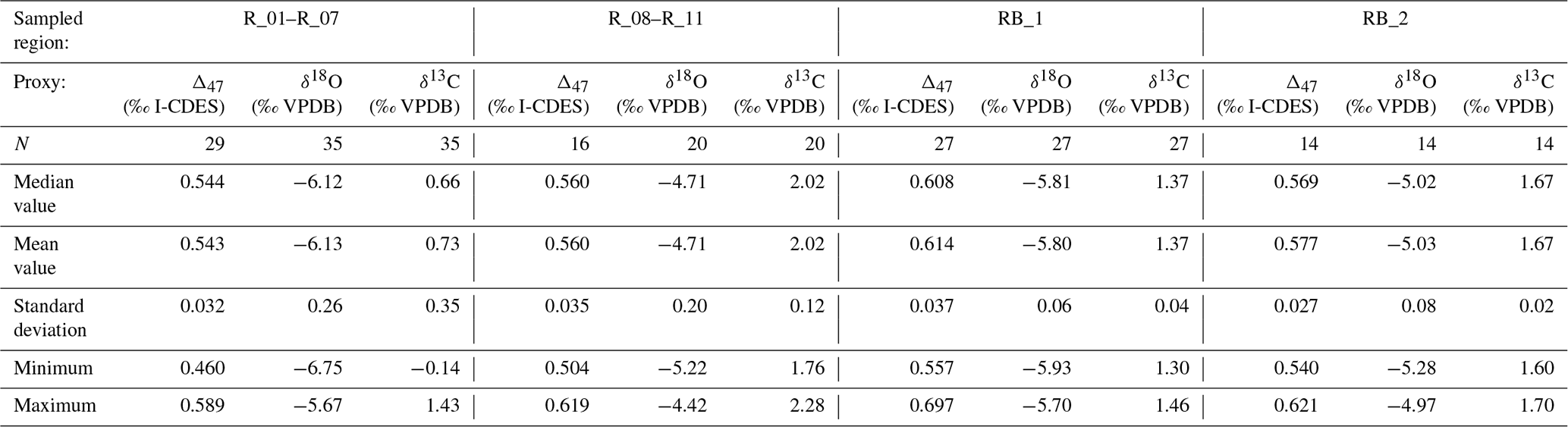
Representative samples from two parallel central pillars of specimen HU-027 were sampled for clumped isotope analysis (see Fig. 2). During sampling, care was taken to avoid the diagenetically altered sections of the shell (Fig. 2C–F). Two areas in HU-027 were drilled for bulk clumped isotope analysis (“RB_1” and “RB_2”; Fig. 2A; see Sect. 2.1), after which samples were drilled from transects in growth direction along one of the pillars exposed in the shell (Fig. 2A). A total of 94 small (70–95 µg) aliquots of calcite powder were reacted with anhydrous (103 %) phosphoric acid in a Kiel IV carbonate device. The resulting CO₂ was cryogenically purified and cleaned using a PoraPak Q trap kept at −40 °C (Petersen et al., 2016b) before being led into a MAT253 or MAT253 PLUS IRMS via a Dual Inlet system. Intensities on masses 44–49 of the CO₂ samples were measured using the Long Integration Dual Inlet mode (Müller et al., 2017) with 400 s integration time against a clean CO₂ working gas (δ¹³C = −2.82 ‰; δ¹⁸O = −4.67 ‰), corrected for the pressure baseline (He et al., 2012). Clumped isotope values (Δ₄₇) were brought into the Intercarb Carbon Dioxide Equilibrium Scale (I-CDES; Bernasconi et al., 2021) using the three ETH standards (ETH-1, ETH-2 and ETH-3) and their accepted values (Bernasconi et al., 2018). Throughout this procedure, samples were corrected with standards whose signal intensities on the mass 44 cup deviated from the intensities of the samples by less than 1 V to prevent any intensity-based offset in the clumped isotope values to bias the result. For samples for which less than 5 intensity-matched standards were available for this correction, the Δ₄₇ value was not considered in the rest of the analysis. The complete analytical system was monitored regarding performance with two independent standards (IAEA-C2, N = 49, and Merck, N = 48), which were treated as samples throughout the measurement procedure. The standard deviations of Δ₄₇ values of these check standards were 0.053 ‰ for IAEA-C2 and 0.039 ‰ for Merck. The reproducibility standard deviations of δ¹³C and δ¹⁸O for IAEA-C2 were 0.05 ‰ and 0.09 ‰ respectively and for Merck the reproducibility standard deviations were 0.09 ‰ and 0.13 ‰ for δ¹³C and δ¹⁸O respectively. Results of clumped and associated stable isotope data are reported in File S2 in the Zenodo repository (de Winter, 2025). A summary of the δ¹³C, δ¹⁸O and Δ₄₇ values organized by the four regions of HU-027 that were sampled (see Fig. 2) is presented in Table 2.

Table 2 Statistics of carbon, oxygen and clumped isotope results organized per sampled region in specimen HU-027.

2.3 Modern bivalve occurrence and climate

To contrast the paleoclimate reconstructions from the above-mentioned multi-proxy dataset, we extracted data on the occurrences of bivalves in modern oceans from the Ocean Biodiversity Information System database (OBIS, 2025). We accessed the OBIS database through the “occurrences” function of the “robis” package (Provoost et al., 2022) and processed the occurrences in the open-source computational software package R (R Core Team, 2023). A total of 2 199 523 occurrences of taxa in the class of Bivalvia were extracted from the database, and their localities were categorized in bins of 2° by 2° based on their latitude and longitude.

Modern seasonal SST ranges across the world oceans were extracted from the Extended Reconstructed Sea Surface Temperature (ERSST) dataset from the National Oceanic and Atmospheric Administration (NOAA; Huang et al., 2017). We extracted monthly data from the years 1981 until 2010 on a 2° by 2° latitude and longitude grid from the ERSST dataset. We extracted the warmest and coldest monthly temperatures from the grid cells that contained reported occurrences of bivalves in the OBIS dataset. This resulted in a distribution of the warmest and coldest monthly temperatures across the living environment of modern bivalves.

2.4 Data processing

Our clumped isotope dataset on specimen HU-027 yielded information about the seasonal spread in temperature and the water oxygen isotopic value (δ¹⁸O_w) experienced by this specimen. We reconstructed these parameters from the Δ₄₇ and δ¹⁸O_c values of the shell carbonate following the clumped isotope-temperature relationship by Daëron and Vermeesch (2023) and the calcite δ¹⁸O_c-δ¹⁸O_w-temperature relationship by Kim and O'Neil (1997). This dataset allowed us to characterize seasonal variability in climate in the Saiwan paleoenvironment. However, since the relatively short δ¹⁸O profile from HU-027 did not allow age modelling and the clumped isotope dataset only sampled one specimen, we augmented the dataset from HU-027 with δ¹⁸O, δ¹³C and trace element data from other specimens (see Sect. 2.2.3) in the same assemblage to study the relationship between temperature and growth rate in Saiwan. To achieve this, we carried out subsequent data processing steps outlined below.

Figure 3 Flowchart of data processing steps carried out for this study.

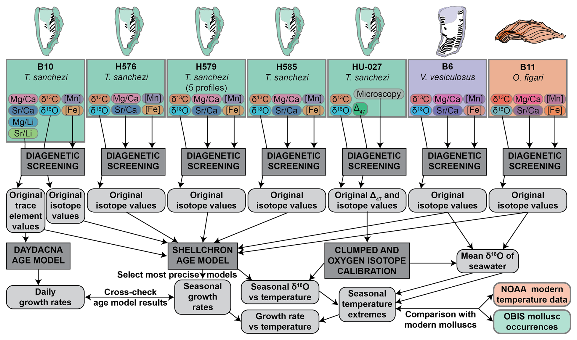
To reconstruct shell growth rates of the molluscs and water temperatures in the Saiwan environment from chemical data measured in the shells, we carried out the following data processing steps (see also the flowchart in Fig. 3):

1. We used concentrations of Mn and Fe and Mg $/$ Ca and Sr $/$ Ca ratios to screen for diagenetic recrystallization of parts of the shells, and remove chemical data from suspicious shell sections for further analysis.

2. We applied the ShellChron age model (de Winter, 2022) to produce internal shell chronologies based on seasonal cyclicity in δ¹⁸O and δ¹³C values through each shell profile.

3. We applied the Daydacna age model (Arndt et al., 2023) to produce internal shell chronologies based on subdaily-scale trace element variability in specimen B10 to verify the result of the ShellChron algorithm.

4. We use a combination of oxygen isotope and clumped isotope data, grouped per location in specimen HU-027 to reconstruct seasonal changes in temperature and δ¹⁸O_w in the Saiwan environment, and how they relate to the oxygen isotope variability in the shells.

5. We use the information about δ¹⁸O_w variability in the environment from clumped isotope data in HU-027 to reconstruct seasonal temperature variability in the Saiwan ecosystem based on all δ¹⁸O profiles.

6. We combine seasonal-scale information about shell growth rates and temperatures to determine the maximum temperature at which the mollusc species mineralized their shell and to quantify the effect of temperature on shell growth rates in Saiwan.

Details on the diagenetic screening are discussed in Sects. 3.2 and 4.1. Assumptions and details regarding all data processing steps are explained below.

2.4.1 Seasonal scale age models using ShellChron

Internal age models were created for all δ¹⁸O and δ¹³C profiles in all specimens except for HU-027, for which the δ¹⁸O and δ¹³C profile was too short to meet the criteria for applying the algorithm (see below), as well as the Mg $/$ Ca and Sr $/$ Ca profiles in T. sanchezi specimen B10 based on the growth rate modelling routine ShellChron (de Winter, 2022). ShellChron approximates the shape of the proxy curve from combinations of sinusoidal proxy and growth rate curves. The routine was adapted after the work by Judd et al. (2017) to function in a sliding window algorithm to provide one age-distance model for the entire profile, preventing breaks and time jumps between growth years. ShellChron can approximate the internal chronology of any proxy-distance record using the following assumptions:

1. The proxy has a (quasi) periodic behaviour over the year. In other words: The proxy exhibits one maximum and one minimum per annual cycle.

2. The mineralization (or growth) rate of the archive over a year can be approximated by a (skewed) sinusoid, with one annual maximum and one minimum (which can be zero).

3. The proxy record contains at least 2 full annual cycles to allow for sufficient overlap between moving windows.

ShellChron estimates the uncertainties of age estimates per datapoint by comparing the results of overlapping windows on the proxy record during the sliding window approach which is applied in the model. Since the proxy-depth record in each window in the ShellChron model is estimated separately using a new combination of proxy and growth rate sinusoid, subsequent age estimates for the same distance value can have different, independent outcomes with respect to relative age estimate. In addition, ShellChron propagates the uncertainty on the distances and proxy values (if provided) using a Monte Carlo approach, resulting in a realistic estimate of the uncertainty on the age determination (de Winter, 2022). For each datapoint, the model thus produces a distribution of ages, from which an uncertainty on the relative age of each datapoint is obtained. These can in turn be averaged to gauge the overall precision of the model outcome. In addition, wide age distributions for the same datapoint are indicative of misidentifications of annual cycles in the δ¹⁸O profile, which cause bifurcations in the model outcome, increasing the spread in age outcomes. Therefore, the overall precision of the ShellChron outcome yields information about the certainty of age modelling and can be used as a benchmark for selecting the most reliable age-distance relationship in a shell. The shell height vs. age relationships estimated using ShellChron for multiple proxy records (δ¹⁸O, δ¹³C and trace element ratios, if available) from each specimen except HU-027, including their uncertainties, are provided in File S3 in the Zenodo repository (de Winter, 2025). The age-distance relationships resulting from the most precise age model for each specimen were used to assign a time of the year to each stable isotope and trace element datapoint used in this study.

2.4.2 Sub-seasonal age model using Daydacna

For T. sanchezi specimen B10, from which subdaily-scale Mg $/$ Ca, Mg $/$ Li, Sr $/$ Ca and Sr $/$ Li data were available (de Winter et al., 2020a), we applied the growth modelling routine Daydacna (Arndt et al., 2023) to verify the ShellChron results and enhance the resolution of the age model. Daydacna uses a wavelet transformation to detect daily rhythms in chemical profiles through mollusc shells and applies a user-guided peak identification routine to find age-depth relationships in the shell on a daily scale. We applied the Daydacna routine on subdaily scale Mg $/$ Ca, Mg $/$ Li, Sr $/$ Ca and Sr $/$ Li records one by one through specimen B10 (see script in File S4 in the Zenodo repository; de Winter, 2025). We compare the results of Daydacna with the results of ShellChron, which are based on annual cycles in δ¹⁸O and δ¹³C profiles and are therefore independent from the Daydacna results based on daily cycles in trace element ratios.

2.4.3 Monthly binning of isotope data

Stable isotope data from profiles through all specimens were cross-referenced with shell age results from ShellChron and Daydacna. Datapoints for which age modelling did not yield a conclusive age (e.g. stable isotope datapoints from locations in between data in trace element profiles) were dated by linear interpolation between surrounding samples for which dates were available. All chemical data were then binned into monthly time bins based on the age models. Monthly bins were assigned by dividing the year into 12 equal time segments, defining boundaries between months based on the day of the year. These monthly time bins were assigned 30 times for each specimen, shifting the boundaries between the months by 1 modelled day for each new assignment. The optimal monthly assignment was subsequently found by picking the option out of 30 in which the months with the highest and lowest mean δ¹⁸O value exhibited the highest difference. This age assignment is assumed to find the highest (least smoothed) seasonal variability in δ¹⁸O, while staying true to the sub-annual growth rate variability exhibited by the specimen as modelled by the ShellChron and Daydacna algorithms.

Note that this monthly binning assumes a total of 365 d in a year, while in reality the number of days per year during the Late Cretaceous was higher (de Winter et al., 2020a). In addition, growth stops may occur which prevent the mollusc from recording one or more days during periods of stress (Jones, 1983), even though no clear signs of these were directly observed in our specimens. However, this difference does not influence the monthly binning since 12 equal parts of the year were considered and the number of days per year assumed in the ShellChron and Daydacna models was also set to 365.

2.4.4 Combining clumped isotope and δ¹⁸O data

To overcome the lack of precise intra-shell age control in HU-027 and place the clumped isotope results in a seasonal context, we grouped the Δ₄₇ and carbonate δ¹⁸O (δ¹⁸O_c) data from specimen HU-027 in four bins according to their sampling location (see Fig. 2 and Table 2). This resulted in a seasonal spread of Δ₄₇, δ¹⁸O_c and δ¹³C values which allowed us to quantify the relationship between δ¹⁸O_c and Δ₄₇ (and therefore temperature and δ¹⁸O_w) in the Saiwan environment.

To verify whether our choice of sampling locations for clumped isotope analysis in specimen HU-027 sampled the full seasonal spread in (clumped) isotopic values, we applied a clustering routine to the carbonate δ¹⁸O (δ¹⁸O_c) and δ¹³C values of HU-027 using K-means and Partitioning Around Medioids (PAM) clustering routines (see File S5 in the Zenodo repository; de Winter, 2025). The K-means routine groups datapoints in the δ¹⁸O_c-δ¹³C space into clusters minimizing the squared Euclidian distance between the points within a cluster using the iterative Hartigan-Wong algorithm coded in the “kmeans” function of the “stats” package in R (R Core Team, 2024; Hartigan and Wong, 1979; R Core Team, 2023). Clustering was repeated on the same dataset using the PAM algorithm (Kaufman and Rousseeuw, 1990) using the “pam” function of the “cluster” package (Maechler, 2024; Maechler and Rousseeuw, 2024).

Because of the strong seasonal cycles in productivity, dissolved inorganic carbon composition, freshwater influx and temperature in shallow marine settings, summer and winter seasons are typically recorded through distinct combined δ¹⁸O_c and δ¹³C signatures in mollusc shells (de Winter et al., 2020c; McConnaughey and Gillikin, 2008; Surge et al., 2001). By combining the statistical clustering approach on δ¹⁸O_c and δ¹³C data with this knowledge of typical seasonal isotopic signatures, we verified the assignment of summer and winter seasons in the geochemical record of HU-027 independent from their sampling location. Note that the assignment of bins in our clumped isotope dataset does not rely on this clustering outcome, as the binning was based primarily on location in the shell and only cross-checked with the statistical clustering.

We modelled the relationship between δ¹⁸O_c, δ¹⁸O_w and clumped isotope-based temperature in the Saiwan environment from the data in specimen HU-027. To do so, we used the relative timing of the four clumped isotope clusters (RB_1 directly preceding R_8–R_11 and RB_2 preceding and partly overlapping with R_1–R_7; see Fig. 2) and the assumption that the warmest and coldest clusters record summer and winter temperatures, respectively, to determine the order of the clumped isotope clusters throughout the year. We then simulated the pathways between consecutive clusters in the δ¹⁸O_c, δ¹⁸O_w and temperature through a Monte Carlo simulation, taking into account the uncertainty on these three parameters within the clusters. We simulated 1000 linear pathways between the clusters consisting of 100 steps while preserving the relationships between δ¹⁸O_c, δ¹⁸O_w and temperature, sampling the start and end points from the uncertainty distributions of the parameters in the clusters.

We then estimated δ¹⁸O_w values for each stable isotope measurement in our compilation for which no clumped isotope values were available using this seasonal δ¹⁸O_c-δ¹⁸O_w relationship. Since the cyclical nature of the seasonal δ¹⁸O_c-δ¹⁸O_w relationship produces non-unique δ¹⁸O_w estimates for any given δ¹⁸O_c value (see Sect. 3.4), we used the seasonal timing of the δ¹⁸O_c datapoints to obtain the most likely δ¹⁸O_w outcome: δ¹⁸O_c values associated with the warm, high-δ¹⁸O_w spring/summer season (before the summer δ¹⁸O_c minimum) were assigned the highest of the two possible δ¹⁸O_w outcomes. Samples associated with the lower temperature and δ¹⁸O_w half of the seasonal cycle (after the summer δ¹⁸O_c minimum) were assigned the lowest of the two possible δ¹⁸O_w outcomes. For the specimens of V. vesiculosus (B6) and O. figari (B11), which exhibit higher δ¹⁸O_c values than the T. sanchezi specimens, δ¹⁸O_w values were assigned based on the seasonal timing of the δ¹⁸O_c values. Temperatures were calculated for all δ¹⁸O_c outcomes in our compilation based on the δ¹⁸O_c measurements and δ¹⁸O_w estimates. We produce monthly temperature and δ¹⁸O_w estimates for each specimen by grouping the data obtained from applying the clumped isotope-derived δ¹⁸O_c-δ¹⁸O_w-temperature relationship on δ¹⁸O_c profiles in monthly bins per specimen.

To test the sensitivity of our δ¹⁸O_w and temperature estimates to the observation that the δ¹⁸O_w varies seasonally following the HU-027 clumped isotope outcomes, we also calculated temperatures for all δ¹⁸O_c profiles using a constant δ¹⁸O_w value equal to the mean δ¹⁸O_w value of the three warmer clusters identified in the clumped isotope dataset from HU-027 (average: −0.25 ‰ VSMOW), excluding the cluster that has a low (−4.61 ± 0.86 ‰ VSMOW) δ¹⁸O_w value. We repeated this test assuming the classical (and seasonally constant) δ¹⁸O_w value of −1 ‰ VSMOW, which is often thought to represent fully marine conditions in a land ice-free climate (Shackleton, 1986). We discuss the impact of the decision not to consider seasonal variability in δ¹⁸O_w values for these specimens in Sect. 4.3.

3 Results

3.1 Stable isotope results

All specimens show distinct periodic patterns in δ¹⁸O_c and δ¹³C values when plotted in growth direction through the shells (Fig. 4). Stable oxygen isotope values (δ¹⁸O_c) in the shells vary between −7.1 ‰ VPDB and −1.5 ‰ VPDB with a mean δ¹⁸O_c value of −5.1 ± 0.9 ‰ VPDB (1σ) for the entire dataset. The lowest mean δ¹⁸O_c values are recorded in T. sanchezi shells (−5.5 ± 0.6 ‰ VPDB; 1σ), with higher values recorded in V. vesiculosus (−4.1 ± 0.6 ‰ VPDB; 1σ) and O. figari (−3.6 ± 0.4 ‰ VPDB; 1σ). Similarly, the lowest mean δ¹³C values are recorded in T. sanchezi (0.7 ± 0.9 ‰ VPDB; 1σ), followed by V. vesiculosus (0.8 ± 0.4 ‰ VPDB; 1σ) and O. figari (1.7 ±  0.6 ‰ VPDB; 1σ).

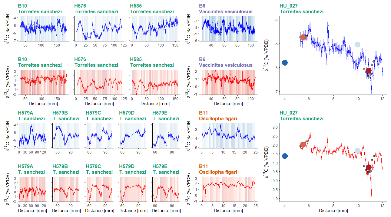
Figure 4 Overview of 11 incrementally sampled stable oxygen (d18Oc; blue) and carbon isotope (δ¹³C; red) profiles: 9 profiles through 5 T. sanchezi specimens, of which 5 parallel profiles through specimen H579 (Top and bottom left and far right, green titles), one profile through V. vesiculosus specimen B6 (Upper middle panel, purple header) and one profile through O. figari specimen B11 (Lower middle panel, orange title). Vertical axes of T. sanchezi profiles in the leftmost panels are equal, while V. vesiculosus, O. figari and T. sanchezi specimen HU-027 have different vertical axes. Records in the lower left panel represent parallel profiles through the same specimen (H579). The shaded background colours represent time of year based on the ShellChron chronologies constructed using these δ¹⁸O_c and δ¹³C profiles, with darker colour indicating samples assigned to days earlier in the year. Black dots in G show δ¹⁸O_c and δ¹³C values associated with clumped isotope measurements in HU-027 and coloured dots and error bars indicate the spread in δ¹⁸O_c and δ¹³C and the location of the material used in clumped clusters presented in Fig. 7.

3.2 Trace element results

Trace element analyses highlight that shells of all three species are generally characterized by low concentrations of Mn and Fe (Fig. 5). T. sanchezi exhibits median Mn concentrations of 38 µg g⁻¹ (average: 50 ± 44 µg g⁻¹, 1σ) and median Fe concentrations of 56 µg g⁻¹ (average: 77 ± 116 µg g⁻¹, 1σ) with a few isolated locations in the shell with concentrations exceeding 300 and 1000 µg g⁻¹ for Mn and Fe, respectively. The carbonate in V. vesiculosus has somewhat higher median Mn concentrations of 176 µg g⁻¹ (average: 192 ± 94 µg g⁻¹, 1σ) and median Fe concentrations of 125 µg g⁻¹ (average: 173 ± 152 µg g⁻¹, 1σ) with some locations showing Mn and Fe concentrations exceeding 500 and 800 µg g⁻¹, respectively. A clear positive trend is observed towards higher Mn and Fe concentrations in V. vesiculosus samples (Fig. 5a). Finally, O. figari has median Mn concentrations of 63 µg g⁻¹ (average: 75 ± 33 µg g⁻¹, 1σ) and much lower median Fe concentrations of 4 µg g⁻¹ (average: 5.7 ± 5.8 µg g⁻¹, 1σ), with maximum Mn and Fe concentrations of 180 and 40 µg g⁻¹, respectively, in some locations.

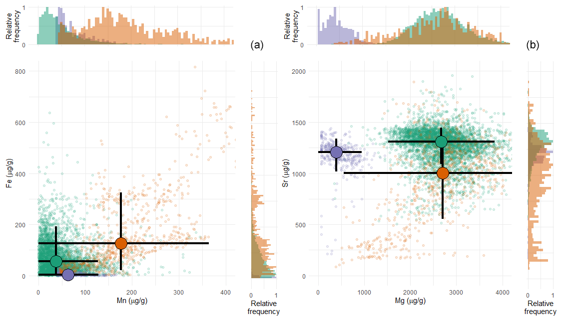
Figure 5 Cross plots of manganese vs. iron (a) and magnesium vs. strontium (b) concentrations in T. sanchezi (green), V. vesiculosus (purple) and O. figari (orange) measured using micro-XRF line scan analysis. Shaded points highlight individual measurements in profiles through the shells while bold black crossed lines highlight median concentration values with 2 standard deviations of the variability per species. Histograms on the edges of the plot show the distribution of concentration values in the dataset per element.

Mg $/$ Ca and Sr $/$ Ca ratios are very similar between T. sanchezi and V. vesiculosus, with mean Mg $/$ Ca ratios of 11.4 ± 2.4 mmol mol⁻¹ (1σ) for T. sanchezi and 11.5 ± 4.8 mmol mol⁻¹ (1σ) for V. vesiculosus and mean Sr $/$ Ca ratios of 1.49 ± 0.21 mmol mol⁻¹ (1σ) for T. sanchezi and 1.09 ± 0.45 mmol mol⁻¹ (1σ) for V. vesiculosus. A subset of the samples from V. vesiculosus exhibit a clear trend towards lower Mg $/$ Ca and Sr $/$ Ca values. O. figari exhibits much lower Mg $/$ Ca values (1.87 ± 1.15 mmol mol⁻¹; 1σ) and Sr $/$ Ca values of 1.36 ± 0.18 mmol mol⁻¹ (1σ).

3.3 Age model results

Applying ShellChron on Mg $/$ Ca, Sr $/$ Ca (only for specimen B10), δ¹⁸O_c and δ¹³C values through all specimens except HU-037 yielded information about the age-distance relationship in the direction of growth through the shells (Fig. 6). These distances in growth direction on cross-sections through the shells were interpreted as proxies for the growth rate of the individual during its life. ShellChron-based age models yield highly consistent age-distance relationships for different T. sanchezi specimens, regardless of whether they are based on Mg $/$ Ca, Sr $/$ Ca, δ¹⁸O_c or δ¹³C records (Fig. 6A). Contrarily, growth models based on δ¹⁸O_c and δ¹³C values in V. vesiculosus and O. figari differed (Fig. 6B–C).

Figure 6 Plot of shell height vs. age in all specimens based on ShellChron modelling on Mg $/$ Ca, Sr $/$ Ca, δ¹⁸O_c and δ¹³C profiles in T. sanchezi (A), δ¹⁸O_c and δ¹³C profiles in V. vesiculosus (B) and δ¹⁸O_c and δ¹³C profiles in O. figari (C). Solid lines represent LOESS smoothed curves (span = 0.2) through the age-height data, with shaded areas indicating uncertainties around the growth models. (D) Comparison between ShellChron results for T. sanchezi specimen B10 profiles (combined chronology from all proxies; black line in panel (A) and Daydacna results on subdaily-scale trace element profiles through the same specimen. Colours of curves and uncertainty envelopes represent the proxy on which age modelling was based (see legends in top-left corners of the panels).

Applying the Daydacna algorithm to trace element records through T. sanchezi specimen B10 (for which subdaily-resolved trace element data is available) yielded independent evidence for the age-depth relationship in shells of T. sanchezi (see Fig. 6D). Except for the Mg $/$ Li record, all age-distance relationships obtained by applying Daydacna on trace element records through specimen B10 closely agree with the age-distance relationship obtained through the combined ShellChron growth models for this and other T. sanchezi specimens. (Fig. 6B). Of the Daydacna results, the model based on Mg $/$ Li ratios deviates most strongly from the other Daydacna results (based on Mg $/$ Ca, Sr $/$ Ca and Sr $/$ Li records) and the stable isotope-based ShellChron age models. The close agreement between these age models generated using different algorithms, based on different environmental cycles (daily vs. seasonal) on different geochemical records through the same specimen, highlights the reproducibility of the age-distance relationship found for our assemblage of T. sanchezi specimens from the Saiwan ecosystem. This lends confidence to the interpretation that the observed rhythms in Mg $/$ Ca, Sr $/$ Ca and Sr $/$ Li records in specimen B10 represent daily cycles (de Winter et al., 2020a) and allows us to refine our age model for this species to quantify growth rates on a monthly scale.

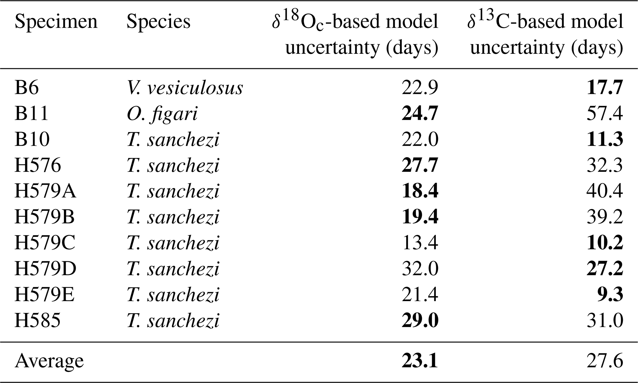
Isotope profiles in Fig. 4 and data on the precision of the ShellChron model outcomes in Table 3 show that the seasonal pattern is in some specimens clearer in δ¹⁸O_c, while others show clearer seasonality in the δ¹³C records. This translates to a better precision of δ¹⁸O_c-based age models in some specimens, while others have better-defined age models based on δ¹³C. On average, the δ¹⁸O_c-based age models are more precise (23.1 d at 95 % confidence level) than the δ¹³C-based age models (27.6 d at 95 % confidence level; see Table 3). To account for inter-specimen differences, we decided to use the most precise growth model (either based on δ¹⁸O_c or δ¹³C) available per specimen for determining the age-distance relationship.

Table 3 Median uncertainty (95 % CL; in days) of growth models based on δ¹⁸O_c and δ¹³C profiles through all sequentially sampled specimens. For each specimen, the most precise age model is highlighted in bold.

3.4 Clumped isotope results

Clumped isotope analysis on T. sanchezi specimen HU-027 yielded a mean Δ₄₇ value of 0.572 ± 0.047 ‰ I-CDES (1σ). The clusters created from the clumped isotope dataset of specimen HU-027 highlight the relationship between δ¹⁸O_c values in T. sanchezi and the temperature and δ¹⁸O_w values reconstructed from clumped isotope thermometry (Fig. 7). Clustering by location in the shell yields maximum reconstructed temperatures in HU-027 of 44.2 ± 4.0 °C and minimum temperatures of 19.2 ± 3.8 °C. These clusters in HU-027 sample a similar or larger spread in δ¹⁸O_c, δ¹³C and Δ₄₇ compared to the statistical clustering approaches that do not take into account the sample location (maximum temperature range: 45.4 ± 17.1 to 24.7 ± 4.3 °C; see File S5 in the Zenodo repository; de Winter, 2025), demonstrating that the sampling strategy successfully resolves the seasonal variability recorded in T. sanchezi specimen HU-027.

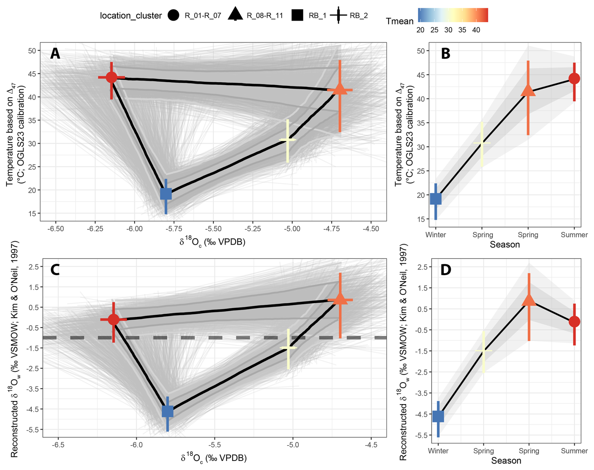
Figure 7 Relationship between temperature and δ¹⁸O_c values (A) and δ¹⁸O_w and δ¹⁸O_c values (C) in T. sanchezi shell based on four clusters of clumped isotope analyses through specimen HU-027 grouped by location of the samples in the shell cross-section (see symbol legend on top). Uncertainties on mean cluster values are reported as 95 % confidence levels. The thin black lines and grey shading highlight individual Monte Carlo simulations (N = 1000) of the most likely shape of the δ¹⁸O_c-temperature and δ¹⁸O_c-δ¹⁸O_w relationship and their 68 % and 95 % confidence levels. The horizontal dashed line in panel (B) indicates the common assumption of a constant δ¹⁸O_w value of −1 ‰ VSMOW throughout the year in the land ice-free Late Cretaceous. Panels (B) and (D) show an interpretation of the seasonality in temperature and δ¹⁸O_w in the Saiwan environment based on these clusters.

Interestingly, while the lowest δ¹⁸O_c values in T. sanchezi are associated with the highest temperatures, as one would expect assuming a constant δ¹⁸O_w value throughout the year, the highest δ¹⁸O_c values do not represent the coldest season. This suggests that the Saiwan environment in the Late Campanian experienced significant seasonal variability in δ¹⁸O_w values. Combining clumped and oxygen isotope data on the clusters shows indeed that they record excursions towards very low δ¹⁸O_w values (−4.63 ± 0.86 ‰ VSMOW) in the coldest season, far off the δ¹⁸O_w value of −1 ‰ VSMOW commonly assumed for past greenhouse periods (Shackleton, 1986).

4 Discussion

4.1 Shell preservation

Ancient shell carbonates, such as the rudists studied here, are known to be susceptible to various forms of diagenetic alteration (Al-Aasm and Veizer, 1986b, a; Brand and Veizer, 1980, 1981; Ullmann and Korte, 2015). Common in carbonate systems, such as the carbonate platforms where the Saiwan rudists were growing, is open-system diagenesis, in which the diagenetic fluid with which the shell carbonate exchanges to alter its chemical and isotopic composition is continuously replaced (Al-Aasm and Veizer, 1986b; Brand and Veizer, 1981). In such systems, the chemical and isotopic composition of carbonates moves away from its original value in an approximately linear trend (mixing line), typically resulting in increased concentrations of trace elements such as Mn and Fe, reduced concentrations of Sr and trends towards lower δ¹⁸O_c values in the carbonate (Al-Aasm and Veizer, 1986b, a).

Our detailed geochemical investigation of specimens B6, B10 and B11 (Figs. 2, 5) highlights low Mn and Fe concentrations (typically < 300 and < 200 µg g⁻¹, respectively, below thresholds used by Schmitt et al., 2022; see Fig. 5) and high Sr concentrations (typically > 1.0 mmol mol⁻¹; see Sect. 3.2), which show a correlated, skewed distribution tailing towards a few locations on the shell where Mn and Fe concentrations are high and Sr concentrations are low, especially in V. vesiculosus specimen B6 (Fig. 5). In V. vesiculosus, the trend of covarying elevated Mn and Fe concentrations and coinciding reductions in Mg $/$ Ca and Sr $/$ Ca clearly shows the imprint of local open-system diagenetic remineralization. Open system diagenesis was observed in isolated localities in these fossil shells, which were avoided during sampling for stable and clumped isotope analysis (see Sect. 2.2.3). The chemical differences between well-preserved sections of the shells of these three taxa are likely to reflect taxon-specific variations in trace element concentrations, which are also common in modern molluscs and may reflect differences in shell microstructures and their associated formation pathways (e.g. Carré et al., 2006; Onuma et al., 1979).

Isotopic compositions of carbon and oxygen are often jointly depleted in diagenetically altered materials due to the exchange of shell carbonate with either isotopically depleted meteoric fluids during early diagenetic alteration (Allan and Matthews, 1990) or exchange with pore fluids under high temperatures (e.g. Brand and Veizer, 1981). However, a positive correlation between δ¹⁸O_c and δ¹⁸C values is not necessarily a reliable indicator of diagenetic alteration (Swart and Oehlert, 2018). Instead, a positive correlation between δ¹⁸O_c and δ¹⁸C values is often observed in modern (non-diagenetically altered) photosymbiotic species, such as tridacnids (Elliot et al., 2009; Killam et al., 2020). Such a correlation has been proposed to be caused by seasonal changes in the isotopic composition of the dissolved inorganic carbon pool due to variability in the activity of photosymbionts in phase with the seasonal effect of temperature on the oxygen isotope composition of the shell (Elliot et al., 2009; McConnaughey and Gillikin, 2008). The fact that T. sanchezi specimens in our dataset exhibit a strong positive correlation between δ¹⁸O_c and δ¹⁸C, while the other species do not, is corroborated by other evidence that T. sanchezi had photosymbionts such as the presence of specific adaptations in the shell thought to facilitate the hosting of photosymbiotic microorganisms in the mantle and the strong expression of diurnal cycles in shell structure and chemistry (see Skelton and Wright, 1987; Steuber, 1999; de Winter et al., 2020a). We therefore disregard this as evidence for open-system diagenesis.

Grain boundary diffusion is another potential diagenetic process that can influence the isotopic composition of biogenic carbonates. This process is rapid on geological timescales (< 100 years) and causes the exchange of oxygen isotopes with pore fluids (Adams et al., 2023; Cisneros-Lazaro et al., 2022; Nooitgedacht et al., 2021). In foraminifera, this process exchanges up to ∼ 3 % of the oxygen in the biomineral (Adams et al., 2023), meaning that even in the presence of strongly isotopically negative pore fluids this process can only change the δ¹⁸O_c value of the biomineral by a few tens of a permille, not enough to fully explain the high temperatures recorded in the fossils in this study.

Finally, our clumped isotope analysis results of specimen HU-027 may be susceptible to solid-state reordering of the clumped isotope signature, a form of closed-system diagenesis which occurs at elevated temperatures (> 100 °C; Chen et al., 2019; Looser et al., 2023; Passey and Henkes, 2012; Stolper and Eiler, 2015). This reordering effect requires large differences between the temperatures in which the carbonate was originally precipitated and the temperatures of the surrounding rocks and, when activated, is likely to affect the entire sample equally rapidly (on geological timescales; Henkes et al., 2014; Stolper and Eiler, 2015). Similarly, heating carbonate samples to 175 °C caused a resetting of the Δ₄₇ value through exchange with internal waters without noticeable change to δ¹⁸O_c values (Nooitgedacht et al., 2021). Given the fact that significant temperature variability is recorded by the clumped isotope dataset from specimen HU-027, and that the recorded temperatures are far from the temperatures needed for the solid-state reordering process to significantly affect isotopic clumping (> 100 °C; Henkes et al., 2014), we feel confident in interpreting the recorded temperatures in terms of the paleoclimate and environment at the Saiwan site.

4.2 Seasonality in temperature and δ¹⁸O_w value in Saiwan

The Monte Carlo simulations of the seasonal δ¹⁸O_c-δ¹⁸O_w-temperature path based on the clumped isotope dataset from specimen HU-027 in Fig. 7 show a statistically significant difference between paleotemperatures and δ¹⁸O_w values between two parts of the annual cycle, especially for the middle range of the δ¹⁸O_c values of (δ¹⁸O_c between −5.0 ‰ and −6.0 ‰ VPDB). Shell increments deposited after the δ¹⁸O_c minimum record lower temperature and δ¹⁸O_w values, while parts of the shell before the δ¹⁸O_c minimum record high temperature and δ¹⁸O_w values. High temperatures are reconstructed for both the extreme ends of the δ¹⁸O_c variability (δ¹⁸O_c < −6.0 and δ¹⁸O_c > −5.0 ‰ VPDB). We interpret this as the signature of a shift in the temperature and δ¹⁸O_w maxima with respect to the δ¹⁸O_c cycle, with a high temperature extreme (44.2 ± 4.0 °C) at the low end of the δ¹⁸O_c cycle, which we interpret as a hot and dry summer season, and a milder temperature maximum (41.4 ± 4.8 °C) at the high end of the δ¹⁸O_c cycle, which we interpret as a warm and dry spring season (Fig. 7B, D). The coldest and wettest season (winter) has such a low δ¹⁸O_w value (−4.64 ± 0.86 ‰ VSMOW) that it is not represented by the highest δ¹⁸O_c values, as would be the case if δ¹⁸O_c would reflect a pure temperature signal (Fig. 7B, D). This interpretation of the seasonality in Saiwan is also consistent with the temporal relationship between the clumped isotope sampling locations in specimen HU-027: Sample RB_1 (winter) comes earliest in the chronology, closely followed by samples R_8–R_11 (spring), and RB_2 (spring) directly precedes R_1–R_7 (summer). The latter two partly overlap later in the chronology (Fig. 2). The result is a seasonality in which the temperature cycle and the hydrological cycle (reconstructed through the δ¹⁸O_w value) are out of phase. The δ¹⁸O_c value of carbonate precipitated under these conditions therefore exhibits hysteresis behaviour (see Fig. 7). Based on the clumped isotope dataset from specimen HU-027 alone, we reconstruct a seasonal sea surface temperature at Saiwan of 19.2 ± 3.8 to 44.2 ± 4.0 °C. The oxygen isotopic composition of the seawater varied from −4.62 ± 0.86 ‰ VSMOW in winter to +0.86 ± 1.6 ‰ VSMOW in summer during the lifetime of specimen HU-027.

4.3 Monthly temperature, δ¹⁸O_w and growth rate at Saiwan

While the strong seasonal variability in δ¹⁸O_w value of the seawater in Saiwan contradicts the typical explanation of δ¹⁸O_c fluctuations in mollusc shells, the assumptions under which the ShellChron model operates (see Sect. 2.4.1) are not violated by this observation. We believe our characterization of seasonal variability in temperature and δ¹⁸O_w value to be realistic for the following reasons:

• Firstly, this temperature distribution over the year, which is offset in phase from the precipitation seasonality, is observed in modern tropical climates, especially those affected by monsoon-like precipitation seasonality.

• Secondly, regardless of the δ¹⁸O_c-temperature relationship, our clumped isotope data show that the maximum temperature is still recorded by the minimum δ¹⁸O_c value. Therefore, the combination of δ¹⁸O_c measurements and seasonal timing based on ShellChron or Daydacna will still assign the correct temperature, δ¹⁸O_w and growth rates to δ¹⁸O_c samples in each part of the year. The nonlinear δ¹⁸O_c-temperature relationship (Fig. 7) therefore does not undermine the growth rate-temperature discussion.

• Thirdly, the comparison between results from the Daydacna algorithm (which is independent from the isotope measurements) with our ShellChron results in specimen B10 shows the same age for this specimen using both independent methods. If ShellChron would under- or overestimate the age of our specimens due to the nonlinear δ¹⁸O_c-temperature relationship, this would cause a mismatch between these results.

• Finally, a previous study carried out on B10 (de Winter et al., 2020a) presents an analysis of the daily layers in specimen B10 using multiple lines of evidence. The result of this study is that this specimen records on average 372 daily layers per δ¹⁸O_c cycle, consistent with astrophysical models of the slow-down of the axial rotation of Earth by friction in the Earth-Moon system, which influences the length of day on geological timescales. The hypothesis that δ¹⁸O_c cyclicity in T. sanchezi represents the full annual cycle (based on ShellChron results) is consistent with this evidence.

Considering the above, we combine information from age models with stable and clumped isotope data from specimen HU-027 to estimate monthly mean temperature, δ¹⁸O_w and growth rate for all specimens in the dataset based on their δ¹⁸O_c values (see Sect. 2.4.4). This further data analysis step works under the assumption that the clumped isotope data from specimen HU-027 samples the seasonal variability in temperature and δ¹⁸O_w in Saiwan. We also assume that the ShellChron age models based on δ¹⁸O_c profiles in the other specimens are accurate enough to reliably distinguish between the hot, high-δ¹⁸O_w and cooler low-δ¹⁸O_w half of the annual cycle, such that the correct δ¹⁸O_w value can be estimated for each δ¹⁸O_c value in the profile and the δ¹⁸O_c value can be used to estimate paleotemperature at that time of the year. Given the uncertainty of ShellChron age models for the δ¹⁸O_c profiles in our compilation (∼ 28 d; see Table 3), we believe that our age models are accurate enough to do this.

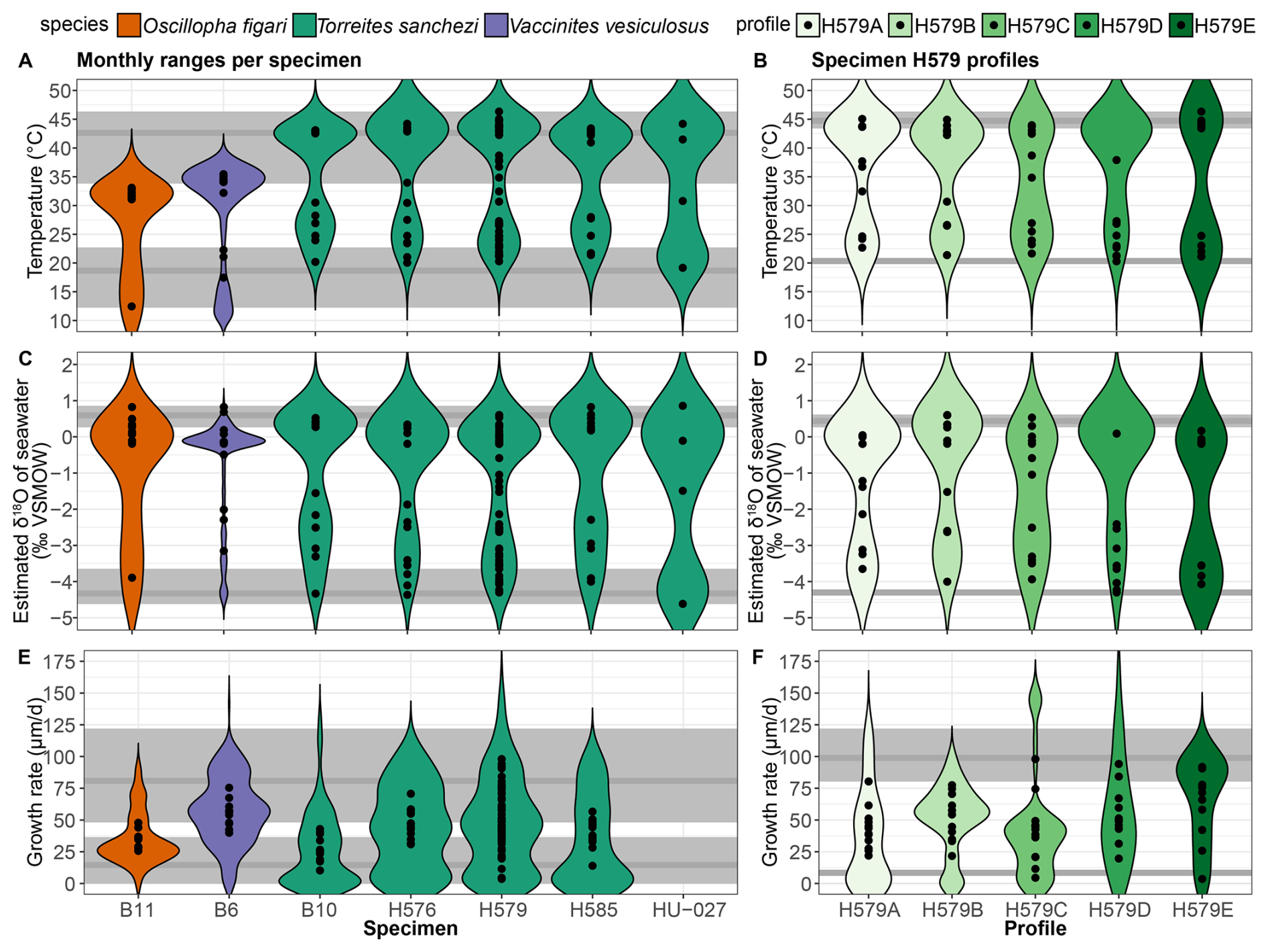
Figure 8 Variability in temperature (A–B), estimated δ¹⁸O_w (C–D) and growth rate (E–F) in all specimens (A, C, E) and in different profiles of specimen H579 (B, D, E). Coloured violin plots indicate the spread in the full dataset, while black symbols indicate monthly mean values. Grey horizontal lines show the highest and lowest monthly mean value, respectively, through the entire dataset (A, C, E) or specimen H579 (B, D, E) with shaded rectangles indicating variability around these values. Note that growth rates could not be estimated for specimen HU-027, and that the black symbols for this specimen in δ¹⁸O_w and temperature plots (A) and (C) indicate values for the four clusters (see Table 1) instead of monthly values.

Table 4 Overview of monthly mean, maximum and minimum estimates of δ¹⁸O_c (in ‰ VPDB), δ¹³C (in ‰ VPDB), temperature (in °C), δ¹⁸O_w (in ‰ VSMOW) and growth rate (in µm d⁻¹) per specimen. Note that temperature is estimated in three ways to test the sensitivity to different assumptions for the value of δ¹⁸O_w: Firstly, by using the δ¹⁸O_w-temperature relationship based on clumped isotope clusters in specimen HU-027 (see Fig. 7). Secondly, by assuming the classical ice-free mean ocean value of −1 ‰ VSMOW. Thirdly, by using the mean δ¹⁸O_w value based on the heaviest three clumped isotope clusters in specimen HU-027 (−0.25 ‰ VSMOW; see Fig. 7B). In each temperature column, results for the different δ¹⁸O_c profiles depend on the same assumption of δ¹⁸O_w variability, so these seasonal temperature estimates are not fully independent from each other. Data given for specimen HU-027 highlights the spread in temperature outcomes between the clusters instead of monthly values.

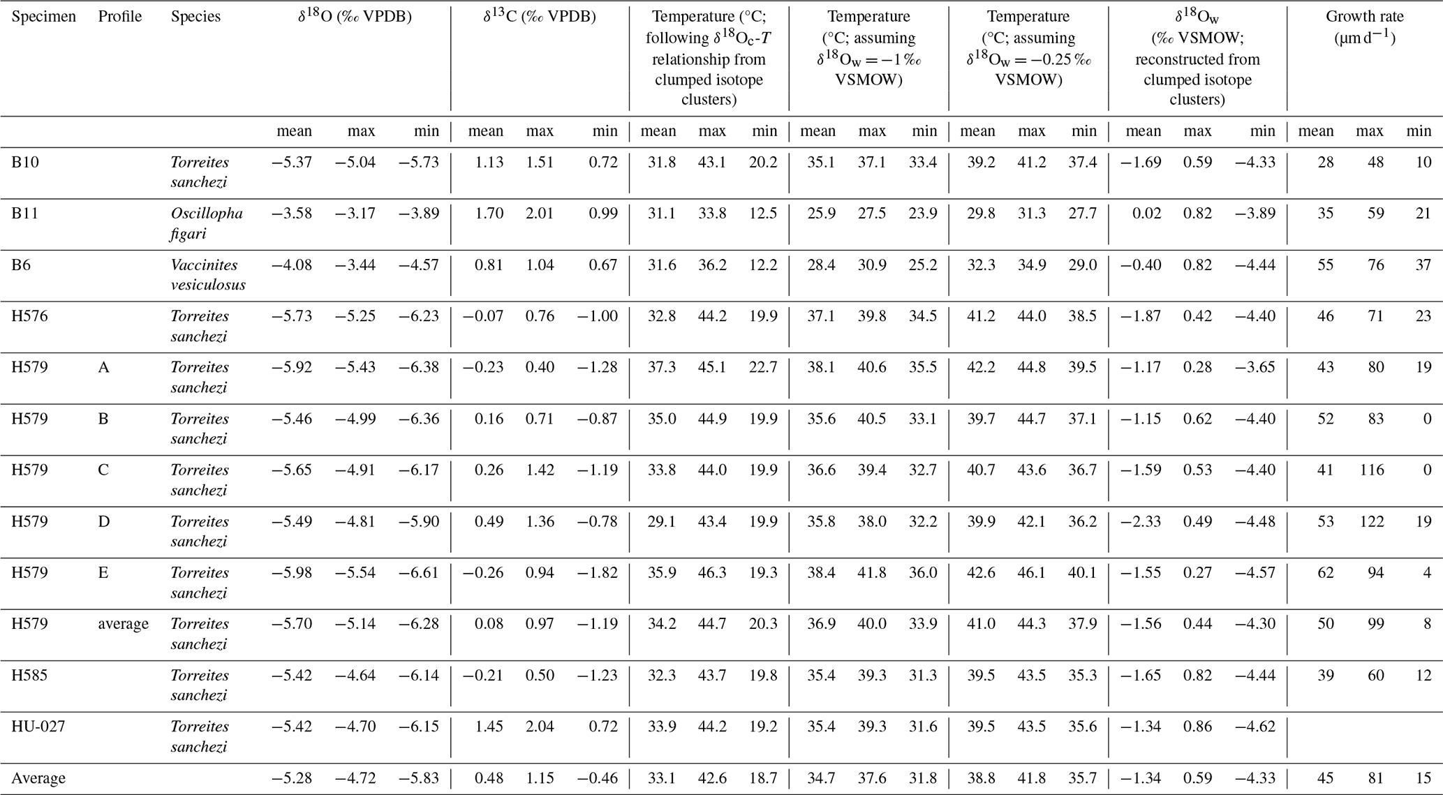
Figure 8 shows the spread in monthly temperature, δ¹⁸O_w and growth rate averages. Table 4 also highlights the implications of the seasonal variability in δ¹⁸O_w throughout the year in the Saiwan environment (see Fig. 7C–D): Correcting δ¹⁸O_c values for δ¹⁸O_w variability in all specimens yields an average coldest month mean temperature (CMMT) of 18.7 ± 3.8 °C and a warmest month mean temperature (WMMT) of 42.6 ± 4.0 °C for the entire dataset. Mean annual average temperatures were 33.1 ± 4.6 °C. The uncertainties on these estimates are propagated from the uncertainties of the lowest and highest temperature clusters in the clumped isotope dataset (see Table 2 and Fig. 7).

Using the classic assumption of a seasonally constant δ¹⁸O_w value of −1 ‰ VSMOW yields a considerably narrower and warmer monthly temperature range (CMMT–WMMT) of 31.8–37.6 °C. Alternatively, when we exclude the coldest clumped isotope cluster in the HU-027 dataset, which has a very low δ¹⁸O_w value of −4.62 ± 0.86 ‰ VSMOW (Fig. 7), and might therefore be biased by a strong seasonal influx of meteoric water, and assume the mean of the other three clusters (−0.25 ‰ VSMOW) as a constant δ¹⁸O_w value, the CMMT-WMMT range becomes 35.7–41.8 °C. Recent studies demonstrated that the assumption of seasonally constant δ¹⁸O_w values in shallow marine environments often leads to an underestimation of the seasonal temperature range from δ¹⁸O_c measurements (e.g. de Winter et al., 2021a). We observe the same effect here and therefore use the seasonal temperature reconstructions that take into account seasonal δ¹⁸O_w variability from our clumped isotope T. sanchezi dataset throughout the remainder of the discussion.

4.4 Inter-species differences

There is a significant difference between the δ¹⁸O_c ranges recorded in V. vesiculosus, O. figari and T. sanchezi in our dataset (see Figs. 8 and 9). When considering the seasonal δ¹⁸O_w variability in Saiwan, the T. sanchezi specimens record significantly higher temperatures in their shells (19.2–45.1 °C range of monthly temperatures, with an average of 33.6 °C) than V. vesiculosus (12.2–36.2 °C; average: 31.6 °C) and O. figari (12.5–33.8 °C; average: 31.1 °C). While the age models allow growth stops, it is possible that some months were not recorded by one or more of these species, reducing the seasonal range. This is also evident from the minimum monthly mean growth rate modelled from some δ¹⁸O_c profiles (e.g. in specimen H579; see Table 4) being zero.

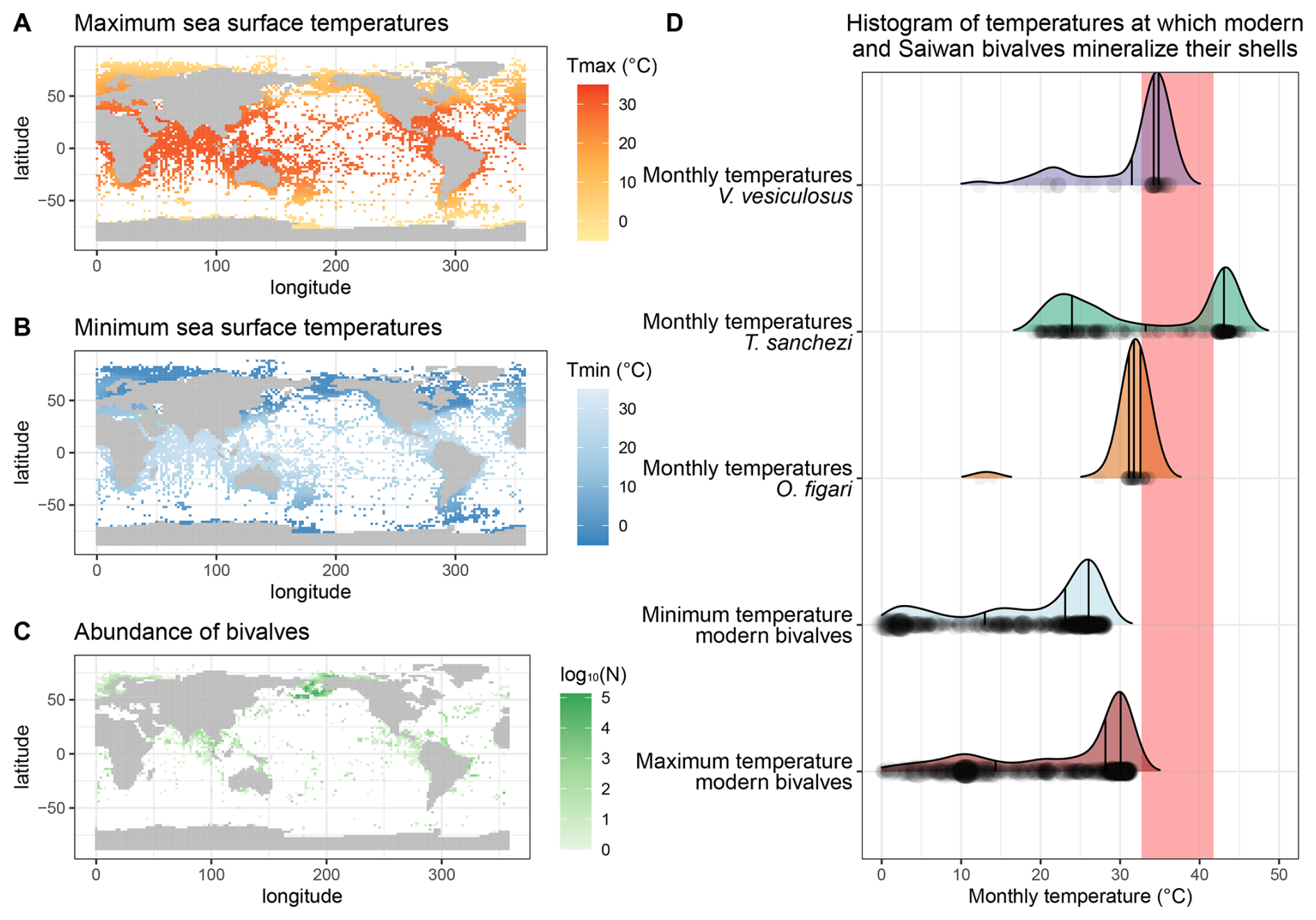
Figure 9 Overview of maximum (A) and minimum (B) modern monthly SST based on the NOAA SST dataset (Huang et al., 2017) at locations of modern bivalve occurrences (C) based on the OBIS dataset (OBIS, 2025) compared with the monthly temperatures reconstructed from the Saiwan fossil molluscs (D). The grey rectangle in panel (D) marks the range of temperature limits for modern bivalves in the hottest shallow marine environment studied in Compton et al. (2007): Roebuck Bay.

Nevertheless, the inter-species difference is surprising, given that these specimens originated from the same biostrome (or directly above, in the case of O. figari; see Fig. 1B–C). The lower temperatures (∼ 2 ‰ higher mean δ¹⁸O_c) recorded in O. figari may be attributed to its slightly higher stratigraphic position. Since the Saiwan site is embedded in a long stratigraphic record and is dated based on ammonite biozones, which yield a dating accuracy on the order of ∼ 100 kyr (Lehmann, 2015), there remains some uncertainty to the (internal) age variability between the units (Kennedy et al., 2000; Schumann, 1995). Therefore, it is possible that the O. figari specimen studied here sampled a different climate and paleoenvironment than the other specimens. This different paleoenvironment may be characterized by a different δ¹⁸O_w value or seasonal δ¹⁸O_w range, resulting in a mild underestimation of paleotemperature and its seasonal range, or a true difference in ambient temperature during the lifetime of the oyster compared to the rudists. Since the mean δ¹⁸O_c value of O. figari is almost 2 ‰ higher than that of T. sanchezi (Table 4), mean annual δ¹⁸O_w would have to have increased by 2 ‰ within a (geologically) very short time interval, given the close stratigraphic relationship between the species, to explain the difference. A plausible way to achieve such a change might be a shift in the seasonal δ¹⁸O_w regime: If the climate in which O. figari grew did not feature the highly δ¹⁸O_w-depleted winter season (see Fig. 7) and instead featured year-round δ¹⁸O_w values close to −0.25 ‰ VSMOW (the mean value of the summer and spring/autumn clusters in HU-027), the difference would explain ∼ 1.2 ‰ of the 2 ‰ difference in the δ¹⁸O_c value. The remaining 0.8 ‰ offset between O. figari and T. sanchezi could then be explained by a drop in mean annual temperature of ∼ 3.5 °C over time based on a typical δ¹⁸O_c-temperature sensitivity of 4.3–4.5 °C ‰⁻¹ (Epstein et al., 1953; Grossman and Ku, 1986; Marchitto et al., 2014). In this scenario, the seasonal temperature range experienced by O. figari was roughly 27.7–31.3 °C (average temperature of 29.8 °C), ∼ 1.3 °C lower than the average temperature recorded by O. figari when accounting for the δ¹⁸O_w seasonality reconstructed by clumped isotope analysis in specimen HU-027, but with a significantly reduced seasonal variability (Table 4). Note that this constant δ¹⁸O_w scenario would also significantly increase the estimated winter temperatures from O. figari, which are very low (12.5 °C; see Table 4) when applying the δ¹⁸O_w seasonality from our clumped isotope data. We therefore consider it likely that the strong drop in temperature and δ¹⁸O_w value that characterized the winter season in Saiwan may not be recorded in O. figari even if it occurred in the climate and environment of O. figari. The temperature distribution in Fig. 9D further confirms this by showing that these exceptionally low winter temperatures in O. figari are represented by a small fraction of the data from this specimen, while the majority of the samples record estimated temperatures between 25 and 35 °C.

This stratigraphic argument cannot explain the temperature differences between V. vesiculosus and T. sanchezi, since they were sampled in life position from the same biostrome. Given the rapid growth of these organisms (de Winter et al., 2017b, 2020b) and the rapid build-up and succession of the biostromes they are found in Gili et al. (1995), Gili and Skelton (2000), and Ross and Skelton (1993), it seems likely that these organisms lived within geologically short time periods from each other (conservatively less than 1000 years), and therefore sampled a similar climate in the Saiwan region. This seems plausible considering the comparatively large overlap in the frequency distribution of temperatures recorded by both species (Table 4; Fig. 9D). The growth rate of V. vesiculosus was on average similar to that of T. sanchezi (see Table 4 and Fig. 8E) and the spatial sampling resolution in V. vesiculosus (250 µm) was often higher than that in T. sanchezi shells (∼ 100–500 µm (de Winter et al., 2017b). Thus, it seems unlikely that the differences between the seasonal ranges obtained from the shells of both species can be attributed to undersampling of the full recorded temperature of V. vesiculosus, a source of variability discussed in Goodwin et al. (2003), Judd et al. (2017), and de Winter et al. (2021b). Applying the high seasonal range in δ¹⁸O_w observed in HU-027, the maximum monthly temperature recorded by V. vesiculosus (36.2 °C) is at least 5° lower than the maximum monthly temperatures recorded in the T. sanchezi specimens (> 43 °C in all specimens, average of 44 °C; Table 4). At the same time, mean annual temperatures in V. vesiculosus (31.6 °C) and T. sanchezi (33.0 °C) differ by less than 1.5°. As in O. figari, winter temperatures in V. vesiculosus are exceptionally low compared to temperature ranges in other specimens in the assemblage (Table 4) and the temperature distribution in this specimen (Fig. 9D). This is a consequence of the fact that winter datapoints in the V. vesiculosus dataset are associated with the very low δ¹⁸O_w values reconstructed from the winter datapoints in the clumped isotope dataset, resulting in low temperature estimates when applied on the δ¹⁸O_c values measured in V. vesiculosus. Since all T. sanchezi specimens yield consistent winter temperatures of ∼ 20 °C, we consider it plausible that V. vesiculosus did not record the seasonally low δ¹⁸O_w conditions and conclude that winter SSTs in Saiwan are more accurately estimated by the T. sanchezi data (19–20 °C).

The growth rate of T. sanchezi specimens is diminished when the range of maximum tolerable temperatures (upper thermal limits) for modern bivalves occurring in hot, shallow marine settings (Roebuck Bay, Australia, tolerable thermal range: 32.7–41.8 °C; Compton et al., 2007) is reached or exceeded (see File S6 in the Zenodo repository; de Winter, 2025). While the frequency of temperatures recorded by V. vesiculosus and O. figari specimens in our dataset decreases when these maximum tolerable temperatures are reached (Fig. 9), temperatures recorded in T. sanchezi specimens regularly exceed modern temperature maxima. Higher temperatures recorded in T. sanchezi specimens suggest that the upper thermal tolerance of this species may exceed those recorded in modern bivalves and that T. sanchezi had a higher temperature tolerance than V. vesiculosus and O. figari.

This conclusion is further supported by the observation that almost all studied T. sanchezi specimens record a monthly temperature range that exceeds that of V. vesiculosus (and O. figari; Table 4) and that the monthly temperature range recorded by T. sanchezi specimens is consistent (see Fig. 8B and Table 4). The fact that all T. sanchezi specimens together record over 30 years of seasonality with consistently low summer δ¹⁸O_c values (monthly minima of −5.7 ‰ VPDB or lower, corresponding to maximum monthly temperatures > 40 °C; see Fig. 3 and Table 4) also shows that these conditions were not isolated events but a persistent feature of the local climate in Saiwan during the Campanian. Finally, daily rhythms in the shell chemistry of the large T. sanchezi specimen B11 have previously revealed that this specimen likely grew year-round, and thus recorded the full seasonal temperature cycle (de Winter et al., 2020a).

An important limitation to this inter-species paleoclimate comparison is that, while the δ¹⁸O_c profiles presented here record independent records of seasonal variability in different specimens, the interpretation of this δ¹⁸O_c variability in terms of paleotemperature relies on clumped isotope data collected in one specimen (HU-027). Our assumption that all rudist specimens occurred in the same biostrome and sampled a highly similar climate allows us to use the seasonal δ¹⁸O_w structure inferred from the clumped isotope dataset in HU-027 to obtain temperature seasonality from δ¹⁸O_c profiles. Therefore, the temperature reconstructions from different δ¹⁸O_c profiles are not fully independent.

4.5 Campanian temperature extremes compared to modern climates – Implications for temperature tolerance in past shallow marine environments

Figure 9A–C presents an overview of the data on the occurrence of modern bivalves from the OBIS dataset (OBIS, 2025) cross-referenced with the monthly temperatures in these modern locations based on NOAA SST data (Huang et al., 2017) for the years 1981–2010. The lowest monthly temperature in environments containing modern bivalve recordings is −1.8 °C. The maximum SST of the warmest month recorded in the NOAA dataset at any location in which modern bivalves are reported is 34.1 °C. Based on the combination of these datasets, it becomes clear that the Saiwan environment was warmer than any shallow marine environment that sustains bivalves in the modern world (Fig. 9D). The range of temperatures experienced by bivalves in the warmest setting studied by Compton et al. (2007; 32.7–41.8 °C) is frequently exceeded in the Saiwan environment, according to the over 4 °C higher mean WMMT estimated from our data (42.6 ± 4.0 °C; Table 4; Fig. 8A). The warmest monthly temperatures in the Saiwan environment thus commonly exceed the maximum monthly temperatures in the living environments of modern bivalves, even when we consider the mean warmest monthly temperature for all specimens instead of the monthly extremes recorded by some T. sanchezi specimens in our dataset (44 °C). When we consider that bivalves are known to stop growing their shell during stressful periods in the year (e.g. winter in most modern bivalves; (Ivany, 2012) and summer in some hotter climates (Buick and Ivany, 2004)), it may be possible (though perhaps unlikely) that the seasonal ranges recorded in our specimens from Saiwan underestimate the true seasonal temperature range in this paleo-environment.

Our clumped isotope data corroborates evidence based on stable oxygen isotope profiles through low-latitude Tethyan rudists (with assumptions of constant seawater δ¹⁸O_w value; e.g. Steuber et al., 2005; de Winter et al., 2017b) that shallow seas in the Cretaceous Tethys Ocean margins warmed up to temperatures unseen in modern climates (Fig. 9), but are not unheard of in the fossil record (e.g. Paleocene-Eocene Thermal Maximum tropical mean annual SSTs > 40 °C; Aze et al., 2014). Clumped isotope data from T. sanchezi specimen HU-027 also reveals that assumptions of year-round constant δ¹⁸O_w value can be very far off from the true δ¹⁸O_w seasonality: in the Saiwan site, the coldest season recorded in HU-027 is characterized by a mean δ¹⁸O_w value of −4.62 ± 0.86 ‰ VSMOW, which is more than 5 ‰ lighter than the mean δ¹⁸O_w value during the warmest season (0.86 ± 1.61 ‰ VSMOW). If δ¹⁸O_w would be considered constant year-round (e.g. −1 ‰ VSMOW), δ¹⁸O_c-based temperature reconstructions would underestimate the true seasonality at this site during the Campanian by over 10 °C (see discussion in Sect. 4.3 and results in Table 4). Our data instead shows that the low-latitude Saiwan paleoenvironment experienced a higher seasonal temperature range than the roughly contemporary (78 Ma) higher mid-latitudes of the Campanian boreal chalk sea recorded in shells from the Kristianstad basin (18.7 ± 3.8–42.6 ± 4.0 °C, or 23.9 ± 6.4 °C seasonal range for Saiwan vs. 15.3 ± 4.8–26.6 ± 5.4 °C, or 11.2 ± 7.3 °C seasonal range for Kristianstad basin), for which seasonal clumped isotope reconstructions were previously presented (de Winter et al., 2021a).

Note that the absolute mean annual temperature for the Saiwan ecosystem (33.1 ± 4.6 °C) was significantly higher than that of the higher latitude Boreal Chalk sea (20.1 ± 1.3 °C; de Winter et al., 2021a), yielding a temperature gradient of ∼ 13 °C over the latitudes 3° S–50° N. The present-day mean annual sea surface temperatures at the closest weather stations to these localities are 8.2 °C (Kristianstad, Sweden, 56° N; Huang et al., 2017; de Winter et al., 2021a) and 27.9 °C (Muscat, Oman, 23° N; NOAA, 2024), yielding a present-day SST gradient of ∼ 19 °C, more than 1.5 × that for the same locations in the Campanian. This result corroborates previous evidence from data and models that the latitudinal temperature gradient was smaller compared to the present-day during periods of warmer climate, such as the Campanian (Amiot et al., 2004; Burgener et al., 2018). However, it must be noticed that the paleolatitudes of these sites are slightly different than their modern latitudes.

The Campanian climate in Saiwan is significantly different from that of present-day Oman, which experiences a sea surface temperature seasonality of 24.2 ± 1.6–31.5 ± 1.6 °C (NOAA, 2024) and a very limited seasonal precipitation range (0–11 mm per month; ECMWF, 2024). The seasonal pattern in temperature and seawater composition in the Campanian is likely caused by large seasonal variability in precipitation, which is common in present-day tropical climates. In this climate, seasons with hot and relatively dry conditions (summers) are interchanged with cooler seasons featuring an influx of isotopically light water, which diluted the shallow seawater at Saiwan or produced a layer of lower salinity waters close to the sea surface, which was recorded by these very shallow-dwelling photosymbiotic rudists.

The above-mentioned conditions make summers in the Saiwan paleoenvironment hot, even for the Campanian with its global mean annual temperature of 20–25 °C (O'Brien et al., 2017). T. sanchezi apparently thrived under these conditions while V. vesiculosus and O. figari stopped producing their shell at temperatures close to those that limit modern shallow marine bivalves (∼ 34 °C; Clarke, 2014; Compton et al., 2007) and perhaps also during the high-precipitation and lower-salinity phases of the winter season. This suggests that T. sanchezi may have been particularly well-adapted to the high seasonality in temperature and precipitation and hot summers in its environment. This hypothesis is further supported by the observation that the genus Torreites occurs exclusively in the late Cretaceous low latitudes (18–29° N) of the near East and middle America (Global Biodiversity Information Facility, 2024). The unexpectedly high seasonal temperature variability in the Saiwan paleoenvironment (18.7 ± 3.8–42.6 ± 4.0 °C; Table 4; Fig. 8) might have provided relief for the Saiwan molluscs, since they were not forced to complete their entire life cycle at exceptionally high temperatures and may have recovered from heat exposure during the cooler seasons.

While the conditions in Campanian Saiwan approach the limits of what has been observed for present-day eukaryotes (Clarke, 2014), recent growth experiments on modern gastropods show that temperatures up to 45 °C can be tolerated by molluscs for limited amounts of time (Prayudi et al., 2024). Organisms that need to withstand these stressful heat conditions often develop specialized proteins and enzymes to continue bodily functions while experiencing close to lethal temperatures (Tehei et al., 2005; Tehei and Zaccai, 2007). While the Campanian fossils studied here do not preserve remnants of these organic molecules, these molluscs probably employed similar strategies to survive through the extreme summer heat. We thus hypothesize that the members of the Saiwan ecosystem (especially T. sanchezi) must have been evolutionarily adapted to its seasonally hot environment. These observations raise the question whether, given enough time, multicellular organisms such as shallow marine bivalves may survive life in hotter climates, and to which degree the thermal tolerance of modern relatives can be used as a reference point for interpreting the fossil record. More research into extreme paleo-communities such as the Saiwan ecosystem is crucial for understanding the evolutionary limits to which metazoans can adapt to warmer climates, how much time is needed to make these adaptations, and whether such adaptation can come in time to save modern shallow marine communities from rapid climate change.