Climate influences on sea salt variability at Mount Brown South, East Antarctica

The Mount Brown South (MBS) ice core in East Antarctica (69° S, 86° E) has produced records of sea salt concentration and snow accumulation for examining past climate. In a previous study, the sea salt concentration, but not snow accumulation, showed a significant, positive relationship with the El Niño–Southern Oscillation (ENSO) from June to November. Here, we use observations and reanalysis data to provide insights into the mechanisms modulating the sea salt concentration record in the ice core, and the previously identified relationship with the tropical Pacific. The MBS site is a wet deposition site, dominated by austral winter and spring snowfall. We find stronger regional circulation anomalies during austral winter (June–August) and focus our analysis on this season. We show that sea salt is likely transported from northeast of MBS via synoptic-scale storms that accompany high precipitation events. These storms and their associated precipitation, show no substantial differences between years of high and low sea salt concentration, so we suggest it is the source of sea salt that differs, rather than the transport mechanism. A teleconnection between the tropical Pacific and high-latitude winds in the vicinity of MBS is identified. Specifically, El Niño events are related to strengthened westerly winds ∼ 60° S, leading to more local sea ice via anomalous Ekman transport in an area to the northeast of the MBS site. Impacts from La Niña are less obvious, showing that there is a non-linear component to this relationship. El Niño–associated strengthened westerly winds in the MBS region could enhance sea salt availability by increasing ocean aerosol spray and/or by increasing sea ice formation, both of which can act as sources of sea salt. This may explain why sea salt concentration, rather than snow accumulation, is most closely related to ENSO variability in the ice core record. Identifying the mechanisms modulating key variables such as sea salts and snow accumulation at ice core sites provides further insights into what these valuable records can decipher about climate variability in the pre-instrumental period.

1 Introduction

Reconstructing past climates is useful for understanding climate variability in the context of anthropogenic climate change since the instrumental climate record is relatively short and spatially incomplete. Paleoclimate reconstructions can complement the observed record through the use of proxies for past climates, which enables context for climate variability and change. This allows for the study of the climate over longer time scales and a wide range of regions, with the aim of potentially constraining future projections (Dee et al., 2016). Palaeoclimate reconstructions rely on adequate spatial coverage to correctly represent spatial variability in the climate response. For this reason, it is important to have a well-dispersed network of ice cores that can be used to understand the long term and region-specific links to drivers of Antarctic climate (Stenni et al., 2017; Li et al., 2021b). The Mount Brown South (MBS) ice core (69.111° S, 86.312° E) was drilled in austral summer 2017/2018 to fill a spatial gap of data for East Antarctica (Crockart et al., 2021). The “main” MBS ice core has a 295 m record spanning 1137 years (873–2009 CE) (Vance et al., 2024).

Crockart et al. (2021) analysed sea salt concentrations in the MBS ice core and found a significant positive correlation between the annual sea salt concentrations and the June–November ENSO (Niño3.4, r=0.457, p=0.002, for 1975–2016). However, the subsequent movement of sea salt to the ice core site, and the underlying dynamical processes of the teleconnection pathway of ENSO, is not yet known. MBS is a wet deposition site (Crockart et al., 2021) which means that the ice core constituents are deposited at the site primarily through precipitation. The snow accumulation rate at the MBS site is recorded in the ice core record and relates to precipitation as well as erosion, ablation and blowing snow (Crockart et al., 2021). It is important to note, Crockart et al. (2021) found the MBS ice core annual snow accumulation rate has no relationship with ENSO. Further work is needed to understand why the MBS sea salt concentration and MBS snow accumulation have different relationships with ENSO. Consideration of the link between sea salt and snow accumulation is important since Jackson et al. (2023) found the MBS ice core to be biased towards extreme precipitation events (days where daily snowfall amount is in the 90th percentile or higher), with these events representing the largest 10 % of all precipitation events but accounting for 52 % of the total annual snowfall at MBS.

Sea salt is an important chemical constituent in ice cores, with possible sources including aerosol spray from the open ocean, frost flowers from newly formed sea ice and the blowing of snow over sea ice, as upward migration of brine from the sea ice to the surface creates higher saline snow (Kaleschke et al., 2004; Frey et al., 2020; Winski et al., 2021; Thomas et al., 2023). There is an inverse relationship between sea salt concentrations and temperature throughout seasonal snow layers as well as between interglacial and glacial periods in ice core records (Petit et al., 1981). Both winter months and glacial periods experience higher sea salt concentrations than summer and interglacial periods. The ionic composition of sea salt aerosol can be used to determine where the source originated from (Rankin et al., 2000; Huang and Jaeglé, 2017; Winski et al., 2021). Huang and Jaeglé (2017) used the chemical transport model GEOS-Chem, validated against in situ observations, and found that in Antarctica submicron sea salt aerosol emissions from blowing snow over sea ice is the most important source of sea salt (2.5 Tg yr⁻¹), followed by the open ocean (1.0 Tg yr⁻¹), and with frost flowers only a minor source of salt (0.25 Tg yr⁻¹). They concluded that blowing snow emissions are largest in regions where persistent strong winds occur over sea ice (this includes the coast near MBS). A critical wind of speed of 8 m s⁻¹ is required to loft snow from the surface (Giordano et al., 2018). The sources of sea salt in Antarctic ice cores are still being debated however the fluctuation of sea ice seems to be important (Abram et al., 2013; Severi et al., 2017; Winski et al., 2021). The relationship varies regionally around Antarctica and the processes involved need to be carefully considered.

When analysing the link between ENSO and Antarctic sea ice, previous studies identify the Antarctic Dipole, which is a simplified statistical description of a quasi-stationary wave in sea ice, sea surface temperature, and surface air temperature (Yuan and Martinson, 2000, 2001; Li et al., 2021a; Lim et al., 2023). The Antarctic Dipole dominates the interannual variability of the sea ice field and the temperature anomalies associated, produce the largest ENSO signal outside of the tropical Pacific (Liu et al., 2002). The Pacific South American (PSA) atmospheric Rossby wave propagation associated with ENSO drives the Antarctic Dipole (Yuan, 2004; Song et al., 2011). During El Niño (La Niña) the Rossby wave creates an arc of low–high–low (high–low–high) pressure anomalies which extends in the south-easterly direction from the tropical Pacific towards Antarctica (Yiu and Maycock, 2019). The Antarctic Dipole and PSA show there are pathways for ENSO to influence Antarctica.

This study aims to provide insights into the mechanisms influencing sea salt concentrations at the MBS site, including local processes as well as understanding processes contributing to the ENSO signal identified by Crockart et al. (2021). There are two main aspects of the processes delivering sea salt to MBS that we investigate:

1. The local processes that could transport sea salt to the ice core. Investigation into specific sources of sea salt at MBS is beyond the scope of this study as there is limited information about the production and transfer of chemical markers from the open ocean and from sea ice to the Antarctic ice sheets (Abram et al., 2013). Rather, here the aim is to relate localised weather and climate circulation patterns to sea salt transport.

2. The dynamical mechanism of the influence of the tropical Pacific on local processes around MBS. Udy et al. (2021) noted that future work is needed to investigate how the surface conditions are preserved in ice core records and that may assist with mechanistic links between the climate and the preservation of the ice core signal.

2 Methods

2.1 Mount Brown South site characteristics

The Mount Brown South site is located at 69.111° S, 86.312° E and 2084 m above sea level (Crockart et al., 2021). Four ice cores were drilled at MBS in the summer of 2017/2018 within 100 m of one another and the Mount Brown South ice core “site average” sea salt record discussed here represents three of the ice cores (the fourth surface core was retained entirely for persistent organic pollutant studies). The three ice core sea salt records show correlations with each other ranging from an r value of 0.43 to 0.59, and each of them exhibits a correlation with the site-averaged record, with an r value greater than 0.8 (Crockart et al., 2021). One of the ice cores has a 295 m record spanning 1137 years (873–2009 CE) (Vance et al., 2024). The raw annual site-averaged sea salt record from Crockart et al. (2021) is used in the analysis. Mean annual surface air temperature for the MBS site is −27.9 °C (Vance et al., 2024). The mean measured annual accumulation rates from 1979 to 2016 at MBS from the three ice cores are averaged to be 0.278 ± 0.040 m w.e. (water equivalent) per year. (Jackson et al., 2023). During different seasons there is only limited variability of prevailing wind speeds and directions shown in model analysis from Vance et al. (2024). The 1979–2016 June–August average magnitude winds off the MBS coast are 5–10 m s⁻¹ (Crockart et al., 2021). Higher precipitation at MBS is linked to local easterly winds and lower precipitation is associated with a southerly element to the winds from the east (Vance et al., 2024). As mentioned above, extreme precipitation events at MBS account for 52 % of annual accumulation (Jackson et al., 2023).

2.2 Data

To look at the climate events related to the modulation of sea salt concentration at MBS we use the data from the MBS ice core that was presented in Crockart et al. (2021). The log–transformed site average mean annual chloride (Cl⁻; sea salt concentration) is detrended from the years 1979–2016 to focus on the observational and reanalysis data period. The data are detrended using linear regression to highlight the interannual variability. It is important to note that at the time of our analysis, only an annually resolved ice core record was available, therefore all analysis on the sea salt concentrations is annually rather than seasonally averaged. However, the annual sea salt concentration is winter dominated (Crockart et al., 2021; Vance et al., 2024) and can thus be considered a “polar winter” record. A winter dominated sea salt record is common in ice core records, this is also the case at Law Dome (Jong et al., 2022).

Gridded sea ice concentration (SIC) from the National Snow and Ice Data Center (NSIDC) Southern Hemisphere version 4 Climate Data Record (Meier et al., 2021) are used to investigate the varying concentration of sea ice as a potential source of sea salt. Data are derived from satellite observations and span 1979–2016. The monthly anomalies are calculated over this period, then the austral winter (JJA), austral spring (SON) and austral winter and spring (JJASON) means are taken.

We use the fifth generation European Centre for Medium-Range Weather Forecasts gridded atmospheric reanalysis of the global climate (ERA5) at monthly resolution to examine atmospheric circulation (Hersbach et al., 2020). We utilise mean sea level pressure (MSLP) and 800 hPa zonal and meridional winds. The wind pressure level of 800 hPa was used since it is close to the surface but does not have interference from the land or ocean surface. These variables are used to investigate the extent of the pressure anomalies propagating from the tropical Pacific and how the circulation around MBS could be influencing the sea ice. The datasets are re-gridded to 1° by 1° over the years 1979–2016. Monthly anomalies are calculated and detrended using linear regression, then the austral winter (JJA), austral spring (SON) and austral winter and spring (JJASON) means are taken.

The ERA5 hourly atmospheric reanalysis data are used to investigate possible mechanisms for the transport of sea salt to the ice core on synoptic timescales, as Jackson et al. (2023) found a high proportion of precipitation at the MBS site to be associated with synoptic–scale storms. The reanalysis datasets are re-gridded to 1° by 1° over the years 1979–2016 for the austral winter (JJA) and austral winter and spring (JJASON). The variables analysed are the precipitation at MBS (69.5° S, 86° E), mean sea level pressure, 800 hPa meridional and 800 hPa zonal wind. There are known biases in ERA5 precipitation data (as well as 2 m air temperature), particularly in data-sparse regions like Antarctica (Roussel et al., 2020; Bromwich et al., 2024). However, ERA5 is considered the best reanalysis for Antarctica, and allows the consideration of circulation, winds and precipitation together (Hassler and Lauer, 2021).

Hadley Centre Global Sea Ice and Sea Surface Temperature (HadISST) gridded sea surface temperature (SST) data (Rayner et al., 2003) are used to investigate the local and remote SST anomalies during high and low sea salt years, including El Niño and La Niña signatures in the tropical Pacific (defined in Sect. 2.3) in the MBS sea salt concentration as well as the tropical influence on MBS local processes. The SST data are re–gridded to 1° by 1° over the years 1979–2016 to match the SIC data temporal resolution. The monthly anomalies are calculated and detrended using linear regression, then the austral winter (JJA), austral spring (SON) and austral winter and spring (JJASON) means are taken. The monthly Southern Oscillation Index (SOI) over 1979–2016 for the austral winter (JJA) is also used to analyse the atmospheric component of the ENSO teleconnection (Bureau of Meteorology, 2025). Anomalies in the tropical Pacific specifically related to ENSO tend to emerge in austral winter (Fogt and Bromwich, 2006).

2.3 Analysis

The annual MBS sea salt concentration data anomalies are split into quartiles. The upper quartile includes the highest 10 sea salt concentration anomalies, and the lower quartile includes the lowest 10 sea salt concentration anomalies (data spanned 38 years from 1979–2016). The Niño3.4 box weighted average (5° N–5° S, 120–170° W) austral winter SST anomalies over the same period are also split into quartiles, also containing 10 data points in the upper and lower quartiles. Composites maps of the upper and lower quartiles are made to analyse how variables averaged over these years differ between the upper and lower quartiles. Composite maps are chosen to analyse the data, as opposed to correlation or regression maps, since composite analysis allows for non–linearities in relationships to be examined. The variables analysed are the SST, SIC, MSLP, 800 hPa zonal wind and 800 hPa meridional wind anomalies. We analyse the upper and lower quartiles at each grid point and use a p value of < 0.1 to conclude that the upper and lower quartiles are statistically not from the same distribution. The Kolmogorov-Smirnov (K-S) test is a non-parametric statistical test used to determine if two samples come from the same distribution or not.

Synoptic–scale storms are investigated as a possible transport mechanism for the sea salt arriving at MBS through wet deposition. Previous studies have noted the extreme precipitation event bias in the MBS ice core (Jackson et al., 2023). Therefore, it is necessary to include precipitation when looking at transport mechanisms. The daily total precipitation for austral winter years in the MBS upper and lower quartiles over the MBS site are calculated using the hourly precipitation data from ERA5. The maximum five precipitation days for each year in the quartiles respectively are defined as extreme precipitation events, and then composite maps for the MBS upper and lower quartiles are created using the five highest precipitation days of each year 800 hPa meridional and zonal wind daily averaged hourly data from ERA5. Analysing the circulation over these 5 d provides an insight into where the winds were travelling from before they arrived at MBS, since back trajectories were beyond the scope of this study.

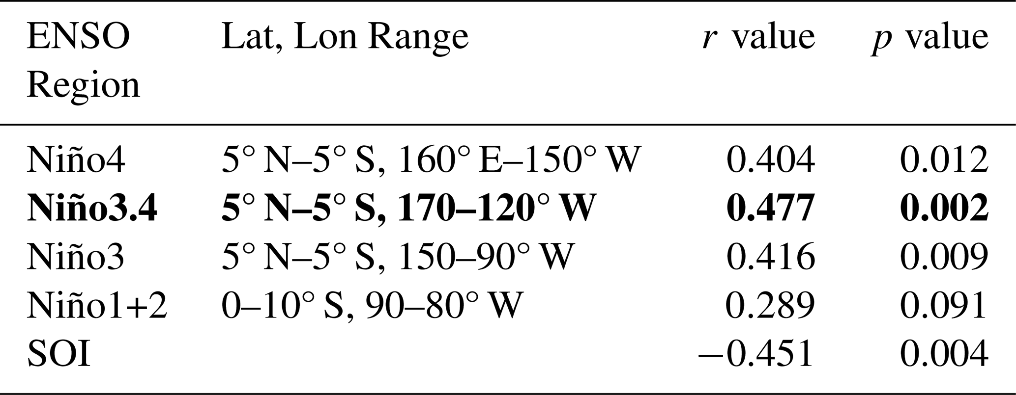
Crockart et al. (2021) found a statistically significant correlation between the sea salt concentration in the MBS ice cores and ENSO during the austral winter and spring (June–November). They found the multivariate ENSO index to have the strongest relationship with the MBS ice core, with an r value of 0.533 for sea salt concentration over 1975–2016 (Crockart et al., 2021, Table 1). The multivariate ENSO index considers the sea level pressure, sea surface temperature, zonal and meridional components of the surface wind, and outgoing longwave radiation over the tropical Pacific basin (30° S–30° N and 100° E–70° W) (Wolter and Timlin, 2011). We analyse the austral winter detrended SST anomalies weighted average over different tropical Pacific boxes, and then focus on the area that has the strongest connection with the MBS sea salt concentration anomaly.

Correlation analyses between annual MBS sea salt anomaly and austral winter-averaged (JJA) Niño4, Niño3.4, Niño3, Niño1+2 SST anomalies (see Table 1 for different ENSO regions latitudes and longitudes), as well as between MBS sea salt anomaly and the winter-averaged (JJA) SIC anomaly northeast of MBS are performed over the period 1979–2016. Note that the northeast SIC region is created over 61–64° S, 90–130° E (see Fig. 3), which is an area approximating the SIC anomalies. Correlations are calculated using Pearson's correlation coefficient. To account for any outliers we use z score analysis, which classifies a z score above three as an outlier (Kannan et al., 2015). The data used in the Pearson's linear correlation coefficient are not greater than three z score.

Table 1 Pearson's correlation coefficients for the MBS sea salt concentrations against four different box averaged SST ENSO regions and SOI, calculated for austral winter (JJA) over 1979–2016. Niño3.4 had the highest r value therefore it is the region used in the analysis (shown in bold text).

3 Results

Section 3.1 first looks at the MBS local processes and compares the high sea salt years to the low sea salt years. Next, we consider the relationship between various ENSO indices and the MBS sea salt record in Sect. 3.2. From there we extend our analysis to consider circulation anomalies during El Niño years and La Niña years, and compare and contrast the relationship between the MBS composites and ENSO composites in Sect. 3.3. Our analysis focuses on June–August however we have included some analysis for September–November and June–November in the appendix (Figs. A3–A9). We have determined that the regional mechanism over SON is weaker than JJA, therefore, we focus on JJA.

3.1 Mount Brown South regional climatology

We first examine the regional conditions around MBS that can influence the modulation of sea salt concentration in the ice core. Past studies have examined the link between sea salt and sea ice conditions, as well as changes in the regional atmospheric circulation (Dixon et al., 2005; Huang and Jaeglé, 2017; Winski et al., 2021). In this section we analyse SIC, MSLP and winds around MBS to investigate links to sea ice or changes to the atmospheric circulation transporting sea salt aerosols from the open ocean to the MBS site.

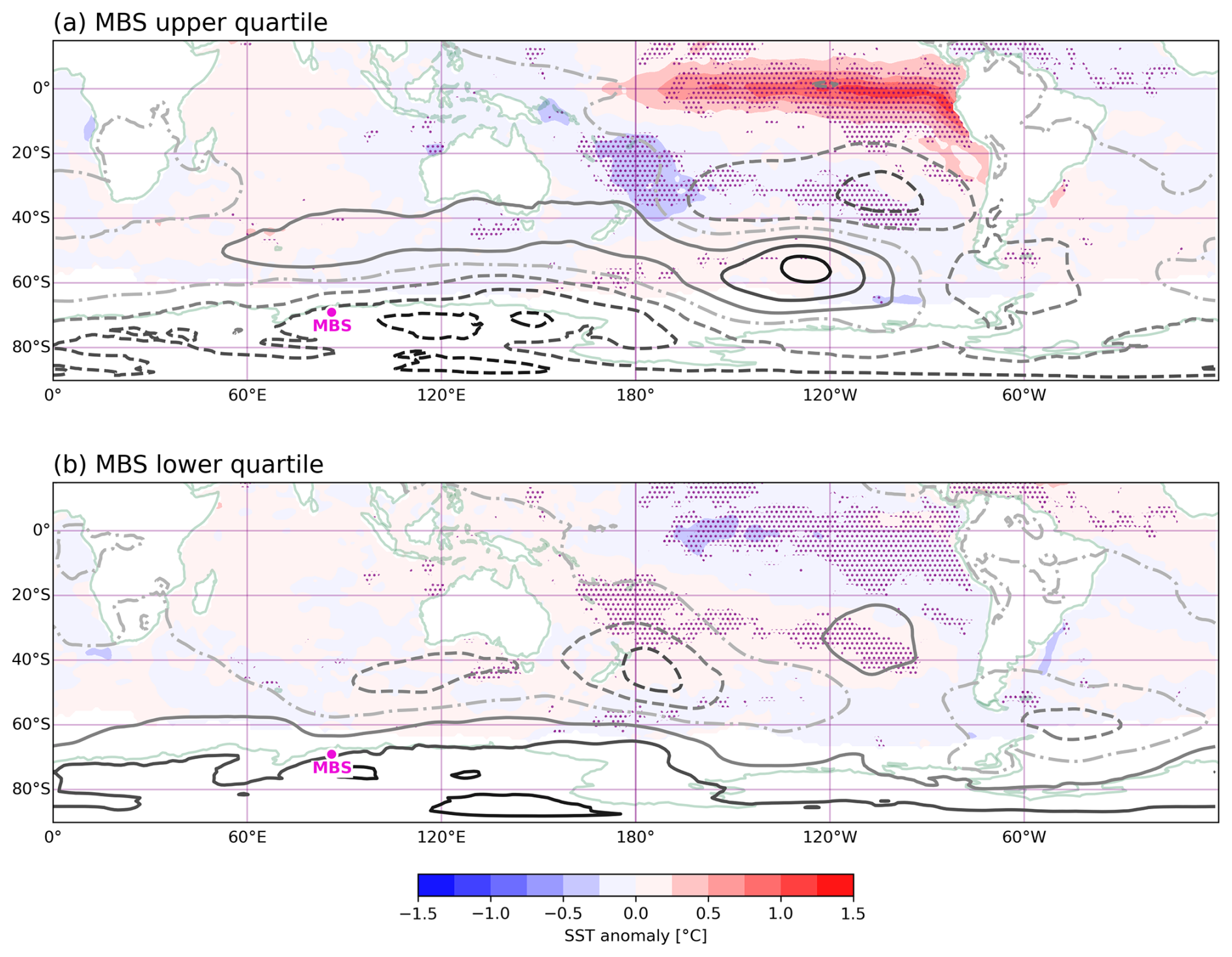
Figure 1 Composite maps of the winter (JJA) sea surface temperature anomaly (shading) and ERA5 mean sea level pressure anomaly (contours) for the Mount Brown South site average (MBS Cl⁻) (a) upper [1982, 1986, 1987, 1993, 1996, 1997, 2009, 2012, 2014, 2015] and (b) lower quartile [1980, 1981, 1983, 1990, 1991, 1995, 1999, 2001, 2010, 2011]. High (low) MSLP anomalies shown by solid (dashed) contours, with darker shades of grey indicating stronger anomalies. The contour line graduations indicate 0.8 hPa. The stippling indicates points where the K-S test p value is < 0.1 for the sea surface temperature anomaly (shading). The fuchsia dot indicates MBS.

The MSLP composite map for the upper MBS sea salt concentration quartile shows a low-pressure anomaly over continental Antarctica, including near MBS (Fig. 1a; contours, Fig. A1a) and a strong El Niño signal in the corresponding SST composite (Fig. 1a; shading). In contrast, in the MBS lower quartile there is a high–pressure anomaly over continental Antarctica near MBS (Fig. 1b; contours, Fig. A1b) and no substantial La Niña signal in the SST pattern (Fig. 1b; shading). This shows that there is a nonlinear relationship between the MBS sea salt concentrations and ENSO, with an El Niño signal but no La Niña signal detected (this relationship is further explored in Sect. 3.2 and 3.3). In the upper quartile composite, the pressure gradient leads to strengthened westerly wind anomalies off the coast of MBS. Conversely, the lower quartile pressure anomaly creates easterly wind anomalies further east off the coast of MBS, compared to the upper quartile (Fig. 1).

Wind anomalies near the MBS region are next analysed to investigate whether there is variance in the source of sea salt (potentially due to sea ice or other changes in sea salt aerosol production) or changes in regional circulation patterns associated with the transport of salts. Z scores of the meridional and zonal wind anomalies are considered, since they are standardized and provide context as to how strong or weak wind anomalies are with respect to the mean.

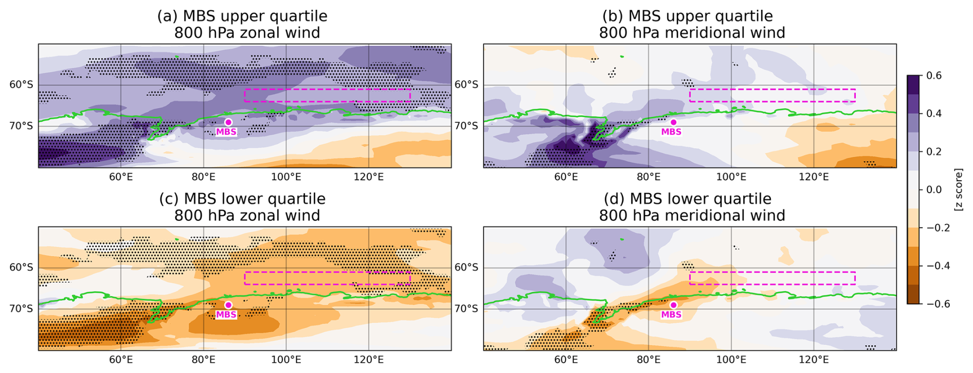
Figure 2 Composite maps of the averaged austral winter (JJA) ERA5 800 hPa meridional and zonal wind anomalies for the Mount Brown South site average (MBS Cl⁻) (a) upper and (c) lower quartile of zonal wind and (b) upper and (d) lower quartile of meridional wind. Upper quartiles (a, b) [1982, 1986, 1987, 1993, 1996, 1997, 2009, 2012, 2014, 2015] and lower quartiles (c, d) [1980, 1981, 1983, 1990, 1991, 1995, 1999, 2001, 2010, 2011]. The stippling indicates points where the K-S test p value is < 0.1. The MBS northeast coast box is highlighted in fuchsia and the fuchsia dot indicates MBS.

The composite maps of 800 hPa wind anomalies shows positive zonal wind anomalies (westerly wind anomalies) along the coast to the east of MBS during years with sea salt concentrations in the upper quartile, and negative zonal wind anomalies (easterly wind anomalies) for the lower quartile (Fig. 2a, c). The direction of these zonal wind anomalies is consistent with the mean sea level pressure anomalies associated with the highest and lowest quartiles shown in Fig. 1. The composite maps of the meridional wind anomalies shows only small changes in the z scores for years in the upper and lower quartiles of MBS sea salt concentrations. Figure 2 shows small, positive meridional wind anomalies (southerly wind anomalies) around the MBS area with high sea salts, and negative meridional wind anomalies (northerly wind anomalies) for years with low sea salt concentrations.

Changes in both the zonal and meridional wind anomalies for the upper and lower quartiles in the MBS region are less than a standard deviation away from the mean. When Petit et al. (1981) explained how changes to the atmospheric circulation related to high sea salt they suggested the need for stronger winds to transport the sea salt from the open ocean to the ice core site since there is increased sea ice extent during this time. From this it would be inferred the meridional wind anomalies should be stronger to transport the sea salt to the ice core site, however there are no substantial local meridional wind anomalies in either the upper or lower quartiles (Fig. 2b, d). There are, however, stronger zonal wind anomalies for the upper quartile (Fig. 2a) that could relate to increased ocean spray increasing the amount of sea salt aerosol in the atmosphere. The opposite is seen in the lower quartile (Fig. 2c) where there are weaker zonal wind anomalies that could relate to decreased ocean spray and therefore decreased amounts of sea salt aerosol in the atmosphere. Together, examination of the anomalous zonal and meridional winds in Fig. 2 suggests that the meridional circulation is not the reason for the modulation of MBS sea salt concentrations. Thus, from this evidence we infer that the modulation of sea salt concentration in the MBS core is likely due to a modulation of sea salt variability linked with the anomalous zonal winds. Increased ocean spray and increased sea ice, both linked with strengthened westerly winds, could act as sources of sea salt.

Next, the SIC is analysed to investigate the changes of sea ice in the MBS region, as newly formed sea ice is a potential source of sea salt aerosol, in addition to blown snow over sea ice covered regions. North and east of the MBS site, a signal of higher SIC anomalies is observed in the upper quartile composite constructed from the MBS sea salt record (Fig. 3a). Conversely, in the lower quartile composite, lower SIC anomalies are observed (Fig. 3b). This is consistent with previous studies that found higher sea salt concentration during winter and glacial periods when sea ice is more prominent (Petit et al., 1981; Pasteris et al., 2014). The MBS northeast coast box averaged SIC is chosen to encompass the high and low SIC anomaly over 61–64° S, 90–130° E (Fig. 3). The correlation between the box-averaged SIC and the MBS sea salt concentration has an r value of 0.448, over the period 1979–2016. This is a statistically significant relationship at the 0.05 % level and shows that when there is higher SIC off the northeast coast of MBS, there is higher sea salt concentration in the MBS ice core. The MBS northeast coast box-averaged SIC is also correlated with the mean zonal and meridional winds in the MBS northeast coast box. The zonal wind and SIC have an r value of 0.350, while the meridional wind and SIC have an r value of 0.555. Both are statistically significant relationships at the 0.05 % level. The mean zonal (meridional) wind is westerly (northerly) and there is a relationship between increased (weakened) strength and higher SIC. These relationships can be understood physically: the correlations are consistent with the mean–state northerly winds transporting sea ice towards the coast and therefore, a weakening in these winds implies less transport towards the coast and thus increased SIC in the outer pack. The strengthening of the mean–state westerly winds will enhance northward Ekman transport of sea ice (increasing SIC), as Ekman transport theory dictates that sea ice will drift 45° to the left of the wind direction (UCAR, 2008; Purich et al., 2016), also increasing SIC in the outer ice pack.

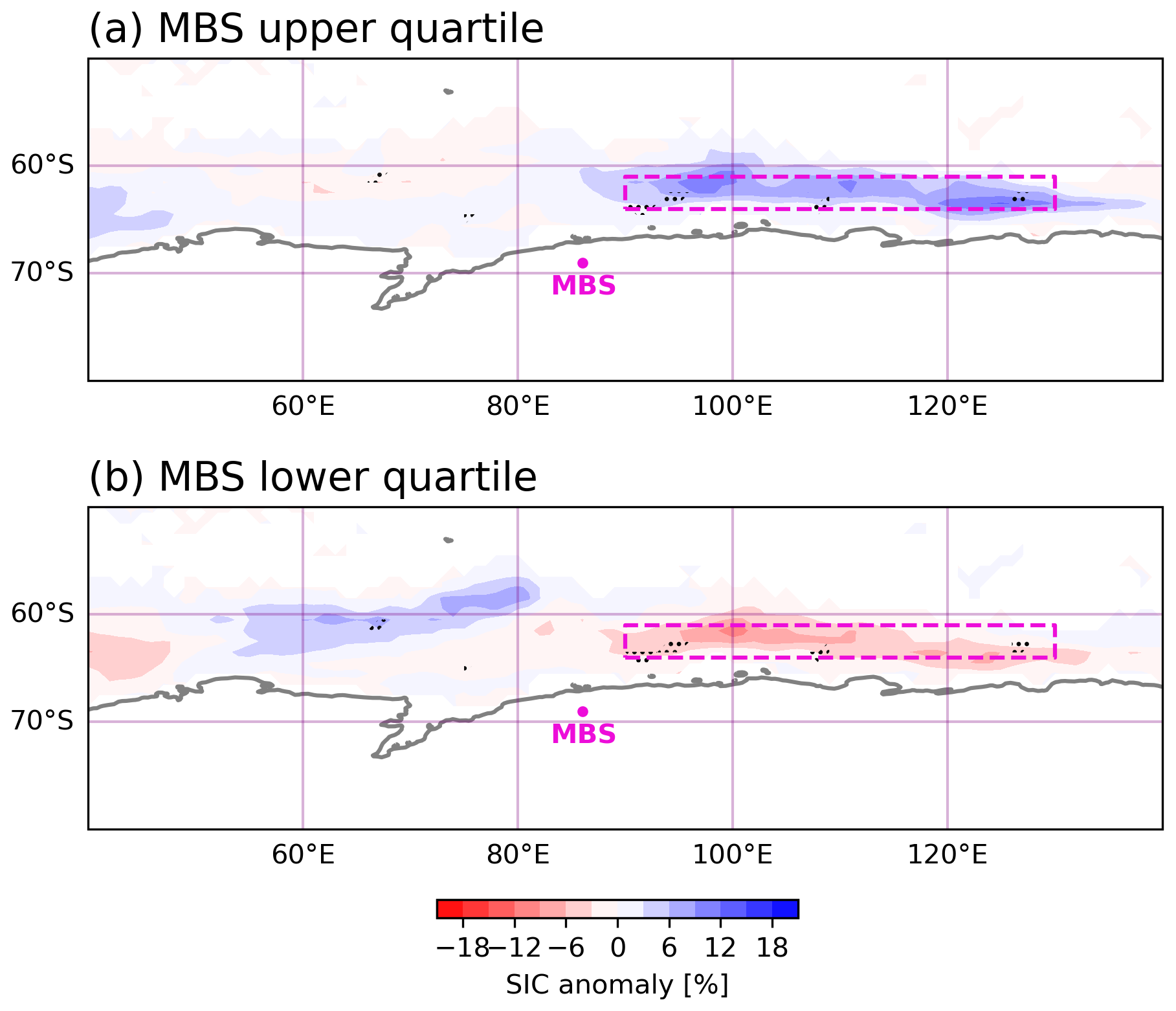
Figure 3 Composite maps of the austral winter (JJA) sea ice concentration for the Mount Brown South site average (MBS Cl⁻) (a) upper [1982, 1986, 1987, 1993, 1996, 1997, 2009, 2012, 2014, 2015] and (b) lower quartile [1980, 1981, 1983, 1990, 1991, 1995, 1999, 2001, 2010, 2011]. The stippling indicates points where the K-S test p value is < 0.1. The MBS northeast coast box (61–64° S, 90–130° E) highlighted by the fuchsia dashed line while the fuchsia dot indicates MBS.

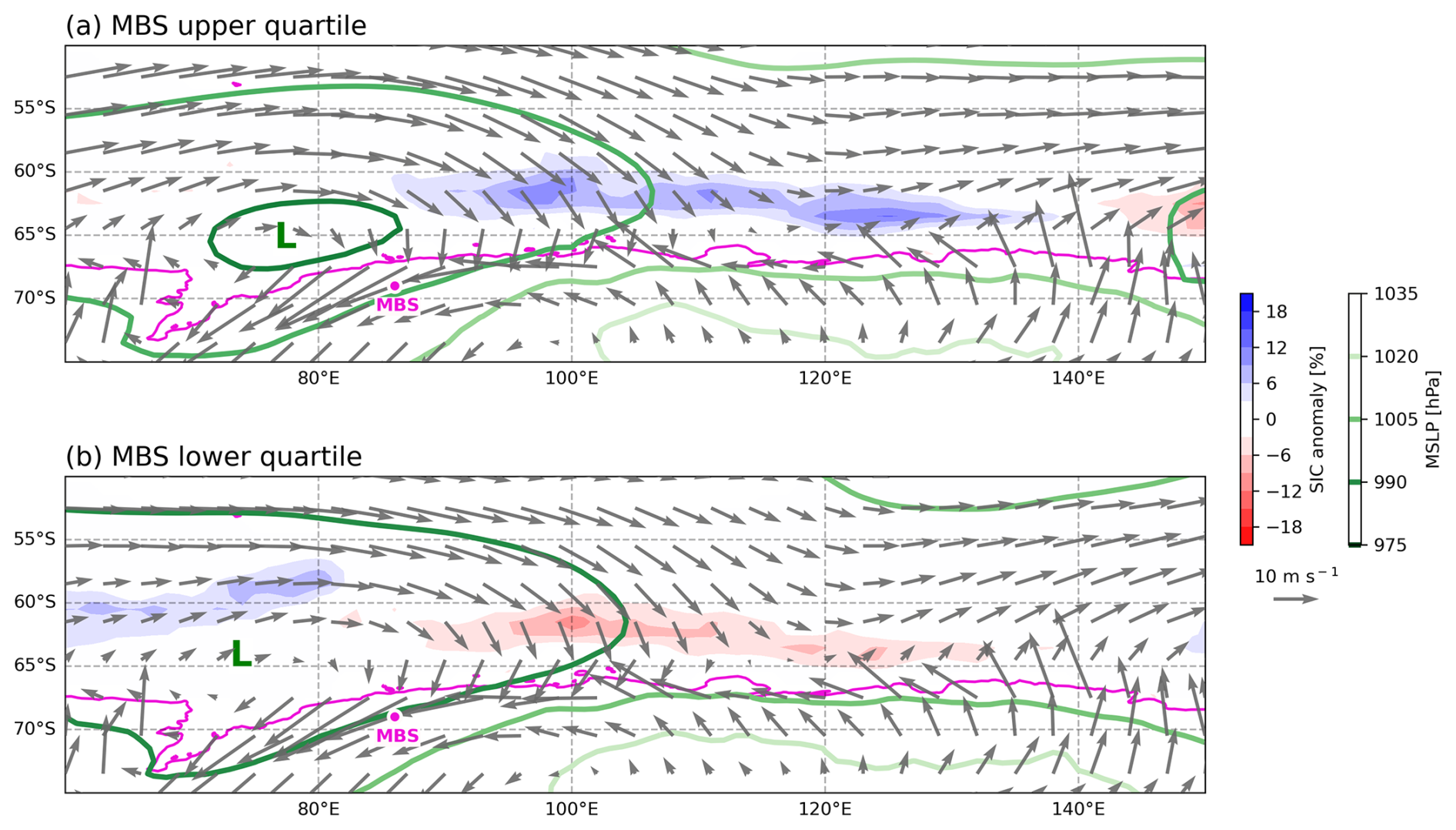
Figure 4 Composite maps of the austral winter (JJA) daily ERA5 mean sea level pressure (contours), daily ERA5 800 hPa mean wind vectors averaged over the 5 maximum precipitation days in austral winter, and (monthly) austral winter (JJA) averaged sea ice concentration (shading) for the Mount Brown South site average (MBS Cl⁻) (a) upper [1982, 1986, 1987, 1993, 1996, 1997, 2009, 2012, 2014, 2015] and (b) MBS lower quartile [1980, 1981, 1983, 1990, 1991, 1995, 1999, 2001, 2010, 2011]. The fuchsia dot indicates MBS.

Daily-scale atmospheric circulation is analysed to investigate the possible mechanism of transport of the sea salt to MBS via moisture–laden weather systems. MBS is a wet deposition site (Crockart et al., 2021; Jackson et al., 2023), and the salt is arriving at the site incorporated in precipitation. As described in Sect. 2.3, the five highest precipitation days from the MBS upper and lower quartiles are analysed. The circulation over these days provides an insight into the trajectory of the air masses prior to their arrival at MBS. In both quartiles and for all storms examined, the 800 hPa winds are cyclonic over the region of the sea ice anomalies, and the MBS site (Fig. 4). This indicates that, for both high and low sea salt deposition conditions, on the days of highest precipitation the winds blow over the northeast coast box sea ice anomaly area, and then blow towards MBS, depositing sea salt aerosol at the site that has been scavenged by precipitation (i.e. wet deposition). In the MBS upper quartile there was a positive SIC anomaly to the northeast of MBS, which infers a larger sea ice area. Provided that sea ice is one of the significant sources of sea salt, this shows that there is a larger source of sea salt at this time, which is consistent with the higher sea salt concentration in the ice core. Conversely, in the MBS lower quartile, the SIC anomaly was negative, which is consistent with less sea ice in the region and, subsequently, a lower sea salt concentration in the ice core. These results support previous studies that have proposed sea ice as a production mechanism for sea salt at Antarctic coastal ice core sites (Thomas et al., 2023). Figure 4 highlights that even though in Fig. 2 the averaged winter wind anomalies for the upper MBS quartile are blowing from MBS to the coast (or weaker winds from the coast to MBS), processes on higher frequency time scales (i.e. synoptic–scale) may be more important for sea salt deposition at MBS compared to monthly circulation patterns. These findings are consistent with the hypothesis from Jackson et al. (2023) that shows that approximately half of annual snowfall at MBS is from these high precipitation storms.

c

3.2 Mount Brown South connection with ENSO

To put the MBS regional atmospheric circulation and sea ice anomalies into context, and given the strong El Niño-like signal in the tropical Pacific in the MBS upper quartile composite (Fig. 1a), we turn our focus to investigate the ENSO influence on the MBS core. We first consider correlations between the annual MBS Cl⁻ concentration (MBS Cl⁻) and different ENSO indices (Table 1). The MBS ice core was not seasonally resolved at the time of this study, therefore austral winter SST in the tropical Pacific was compared to the annually resolved site averaged sea salt concentration. From Table 1, Niño3.4 was shown to have the strongest connection to the MBS sea salt concentration, with an r value of 0.477, which is significant at the 0.2 % level. Therefore, Niño3.4 was used for further analysis.

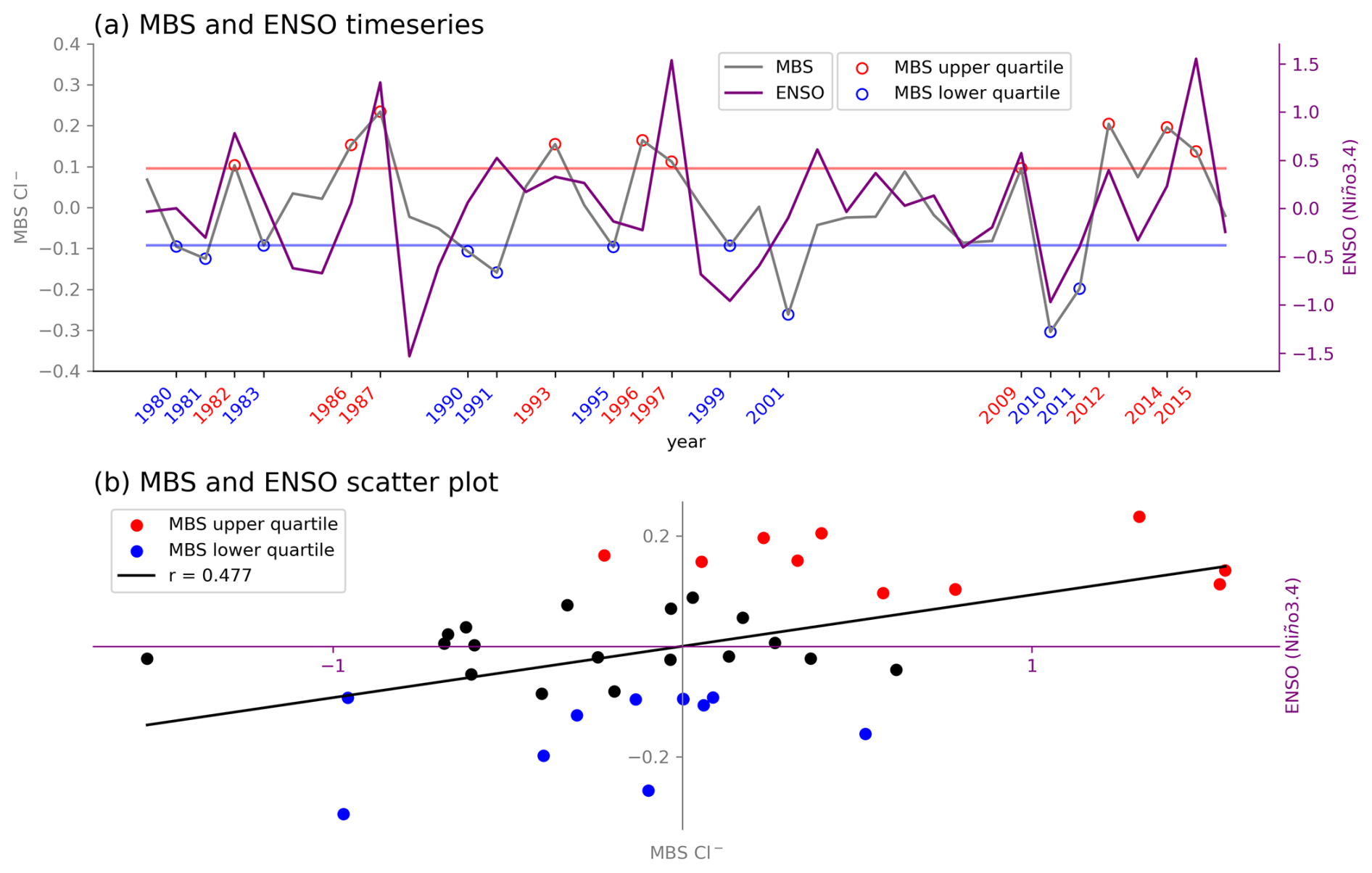
Figure 5 (a) Time series of the annual detrended, log–transformed sea salt concentrations for the Mount Brown South site average (MBS Cl⁻) and the detrended (June–August) El Niño–Southern Oscillation region SST anomalies (Niño3.4). Red line (blue line) indicates the MBS upper (lower) quartile boundary. Red and blue years on the x axis represent the MBS upper and lower quartile years. (b) Scatter plot shows the relationship between the two time series with the MBS upper (lower) quartile highlighted by the red dots (blue dots) based on the period 1979–2016.

Crockart et al. (2021) found a positive correlation of 0.457 over the years 1975–2016 between the MBS sea salt concentration anomalies and the Niño3.4 index for austral winter and spring (Crockart et al., 2021, Table 1). These results were recreated (Fig. 5) using only austral winter for the Niño3.4 SST and over the years 1979–2016. The correlation of 0.477 in Fig. 5 is similar to the correlation from Crockart et al. (2021). While Crockart et al. (2021) found a relationship between ENSO and MBS sea salt concentration, they did not find a statistically significant relationship between ENSO and accumulation in the ice core (r value of 0.147 for Niño3.4; Crockart et al., 2021, Table 1). Therefore, we hypothesise that the ENSO influence on the sea salt variability at MBS could be due to the sea salt aerosol source rather than the deposition dynamics.

3.3 Insights into the mechanisms connecting the El Niño Southern Oscillation to Mount Brown South

Section 3.1 showed a possible connection between the MBS sea salts and regional sea ice, including the transportation mechanism via synoptic-scale storm systems. A statistically significant relationship between the MBS sea salt concentration and Niño3.4 was highlighted in Sect. 3.2. Now, the relationships between the El Niño–Southern Oscillation and those localised mechanisms are investigated in order to provide insights into their hemispheric-scale dynamical connections.

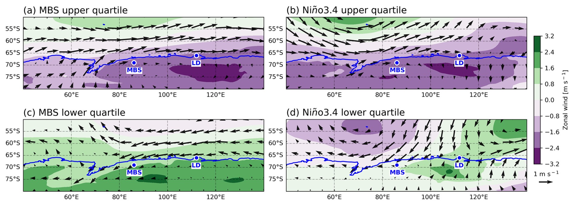
Figure 6 Composite maps of the winter (JJA) ERA5 mean sea level pressure anomaly (shading) with 800 hPa wind vector anomalies overlayed for the Mount Brown South site average (MBS Cl⁻) (a) upper [1982, 1986, 1987, 1993, 1996, 1997, 2009, 2012, 2014, 2015] and (c) lower quartile [1980, 1981, 1983, 1990, 1991, 1995, 1999, 2001, 2010, 2011] and the Niño3.4 (b) upper [1982, 1987, 1991, 1993, 1997, 2002, 2004, 2009, 2012, 2015] and (d) lower quartile [1984, 1985, 1988, 1989, 1998, 1999, 2000, 2007, 2010, 2011]. The blue dots indicate Mount Brown South (MBS) and Law Dome (LD) ice core sites.

First, the regional circulation around MBS is compared between the MBS upper and lower quartiles (Fig. 5a) and the Niño3.4 (Fig. A2). The composite maps of circulation anomalies during the upper quartile of MBS sea salt concentration (Fig. 6a, c) and Niño3.4 quartiles (Fig. 6b, d) show similar wind anomaly vectors for the upper quartiles of each, with both having westerlies to southwesterlies (Fig. 6a, b). Conversely, the lower quartiles of each are less consistent, with the MBS composite showing anomalous easterlies (Fig. 6c), and the Niño3.4 composite showing northeasterlies (Fig. 6d).

The MSLP anomalies for the upper quartiles of MBS and Niño3.4 both show lower pressure anomalies over the land and coast around MBS, and higher-pressure anomalies north off the coast. As for the wind anomalies, the lower quartiles are less consistent, with higher MSLP anomalies over most of the land and coast in the MBS composite. However, the Niño3.4 composite shows a low-pressure anomaly off the west coast of MBS and a high-pressure anomaly off the east coast of MBS. This is a nonlinear response and is consistent with the SST MBS composites in Fig. 1 that show a nonlinear ENSO relation to MBS. This is, the MBS-ENSO relationship is biased towards influences from El Niño, with little influence during La Niña.

The anomalous westerly winds off the MBS coast in the upper quartiles is notable (Fig. 6a, b). As discussed above, this can induce two possible sea salt production mechanisms. Firstly, strengthened westerly winds increase sea salt aerosol lofting from open ocean sea spray. Secondly, in response to the strengthened westerly winds, there will be enhanced northward Ekman transport of sea ice. This ice transport mechanism will increase the SIC on the outer (equatorward) side of the ice pack and increase sea ice formation closer to the coast, with sea ice providing a source of sea salt, either by blowinng snow over sea ice or frost flowers (Frey et al., 2020). The opposite happens during the years with MBS sea salt in the lower quartiles. This is, the easterly wind anomalies (weaker westerly winds) tend to reduce open ocean aerosol lofting, as well as reducing northward Ekman transport of sea ice, decreasing the SIC in the outer ice pack, and limiting the formation of new sea ice in the inner ice pack due to lack of exposed ocean there, thus resulting in an overall lower source of sea salt.

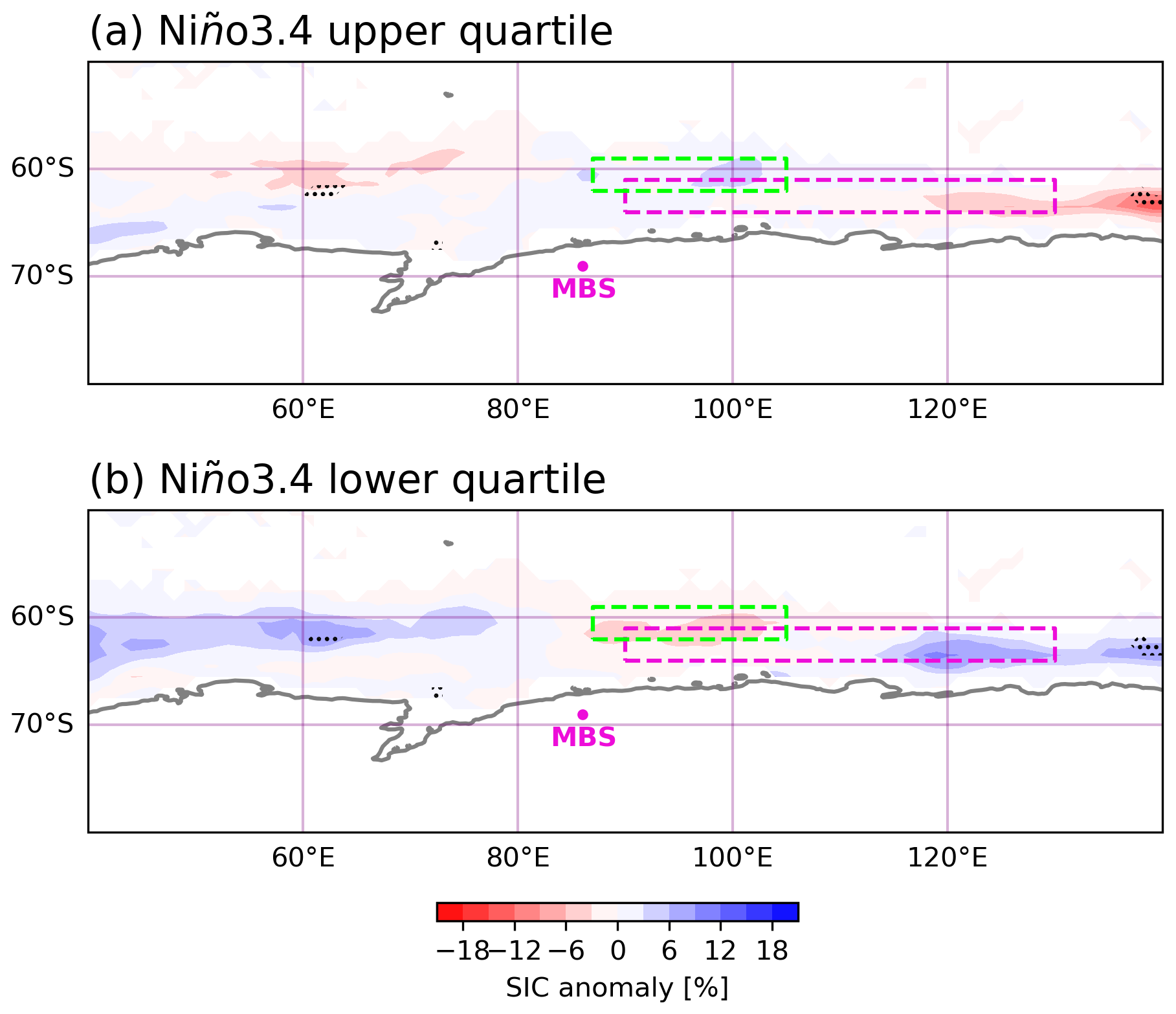
Figure 7 Composite maps of the austral winter (JJA) sea ice concentration for Niño3.4 (a) upper [1982, 1987, 1991, 1993, 1997, 2002, 2004, 2009, 2012, 2015] and (b) lower quartile [1984, 1985, 1988, 1989, 1998, 1999, 2000, 2007, 2010, 2011] with the MBS northeast coast box highlighted in fuchsia dashed line. Lime box (59–62° S, 87–105° W). The fuchsia dot indicates MBS.

When comparing the SIC in Figs. 3 and 7, the ENSO signal in the SIC off the northeast coast of MBS is weak (majority of the region in the fuchsia box in Fig. 7). Yet, there is a small ENSO signal at the far northeast corner of the fuchsia box (highlighted as the lime box in Fig. 7) and an El Niño signal in the SST composite pattern for high MBS Cl⁻ years (Fig. 1a). The lack of a clear ENSO signal in the sea ice directly northeast of MBS could be due to the non-equivalence of SIC (analysed here) and new sea ice formation, which is required for frost flowers, a previously described possible source of sea salt (Rankin et al., 2000).

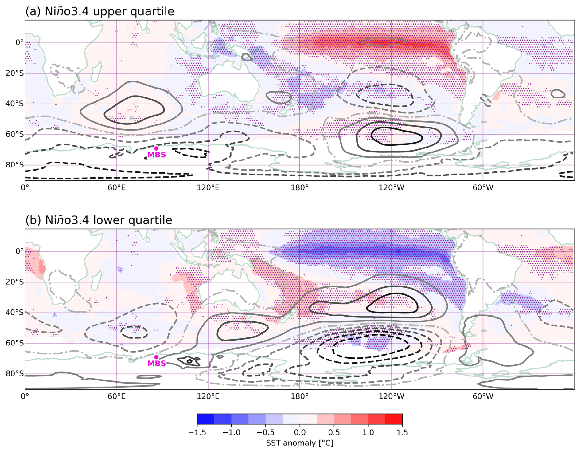
Figure 8 Composite maps of the winter (JJA) sea surface temperature anomaly (shading) and ERA5 mean sea level pressure anomaly (contours) for the Niño3.4 (a) upper [1982, 1987, 1991, 1993, 1997, 2002, 2004, 2009, 2012, 2015] and (b) lower quartile [1984, 1985, 1988, 1989, 1998, 1999, 2000, 2007, 2010, 2011]. High (low) MSLP anomalies shown by solid (dashed) contours. The contour line graduations indicate 0.8 hPa. The fuchsia dot indicates MBS.

Another factor for the difference between the Niño3.4 composites and the MBS composites is the location of westerly wind anomalies. Figure 6 shows that for the MBS upper quartile the westerly winds anomalies stretch to at least 140° E, whereas the Niño3.4 upper quartile westerly winds anomalies become more southerly around 100° E. As described above, the wind anomalies impact the direction of sea ice drift through Ekman transport, and therefore influence where new sea ice forms. The elongated westerly wind anomalies in the MBS upper quartile in Fig. 6 are conducive to the SIC in the MBS upper quartile seen in Fig. 3a.

The low MSLP anomaly over the continent, including near MBS in the Niño3.4 upper quartile (i.e. El Niño-like conditions) in Figs. 8a and A1c is consistent with the low MSLP anomaly in the same position for the MBS upper quartile in Figs. 1a and A1a, although the low pressure in the Niño3.4 upper quartile is not robust like the MBS upper quartile (Appendix Fig. A1). The high MSLP anomaly over the continent, including near MBS in the lower quartile of MBS (Figs. 1b, A1b) is not as clearly seen in the Niño3.4 lower quartile in Figs. 8b, A1d.

The PSA pattern of low–high–low pressure anomalies during El Niño and high–low–high pressure anomalies during La Niña over the southeast Pacific Ocean is seen in both the upper and lower quartiles in Fig. 8. These pressure anomalies are consistent with the known relationship between tropical Pacific SST anomalies, which influences where deep convection occurs in the tropical Pacific (Hoskins and Karoly, 1981), and the propagating Rossby wave trains south and east towards Antarctica (Yiu and Maycock, 2019). When comparing the lower quartiles in Figs. 1 and 8, the PSA is not as well preserved in the MBS lower quartile compared to the lower quartile of the Niño3.4 (i.e. La Niña conditions). The differences between the lower quartiles in Figs. 1 and 8 is another indication of the non–linearity between ENSO and MBS sea salt concentration.

A possible explanation for the nonlinear relationship between MBS sea salt concentration and ENSO is that El Niño is related to westerly wind anomalies off the coast of MBS, which allows for more ocean spray aerosol and new sea ice formation, increasing the source of sea salt available to be transported to MBS. However, La Niña may decrease the amount of ocean aerosol spray but does not have a mechanism for decreasing the amount of sea ice formation compared to a neutral state.

4 Discussion

Figure 9 provides an overview schematic of the possible localised and remote mechanisms that cause high sea salt concentration in the MBS ice core, based on the evidence we present. The figure shows that, locally, there is some evidence that high-precipitation, synoptic-scale systems deliver sea salt to MBS, which is consistent with the role of high-precipitation events to the MBS site (Jackson et al., 2023). The area from which the winds in these high-precipitation synoptic systems originate is over a region of high SIC off the coast to the northeast of the MBS site. We hypothesise that the existence of the area of high sea–ice concentration is related to westerly wind anomalies at the coast promoting the production of sea ice, as well as increased ocean aerosol spray, both of which are conducive to higher sea salt concentrations (Frey et al., 2020; Huang and Jaeglé, 2017). We also suggest that in winter ENSO can influence the winds off the coast of MBS through the known mechanism of the PSA which propagates Rossby waves from the tropical Pacific to Antarctica (Li et al., 2021b). During El Niño the Rossby wave train is more likely to produce a high pressure anomaly off the coast of MBS which creates westerly wind anomalies (Fig. 8). More remotely, this high SIC is weakly related to warm SST anomalies in the tropical Pacific, representing El Niño conditions.

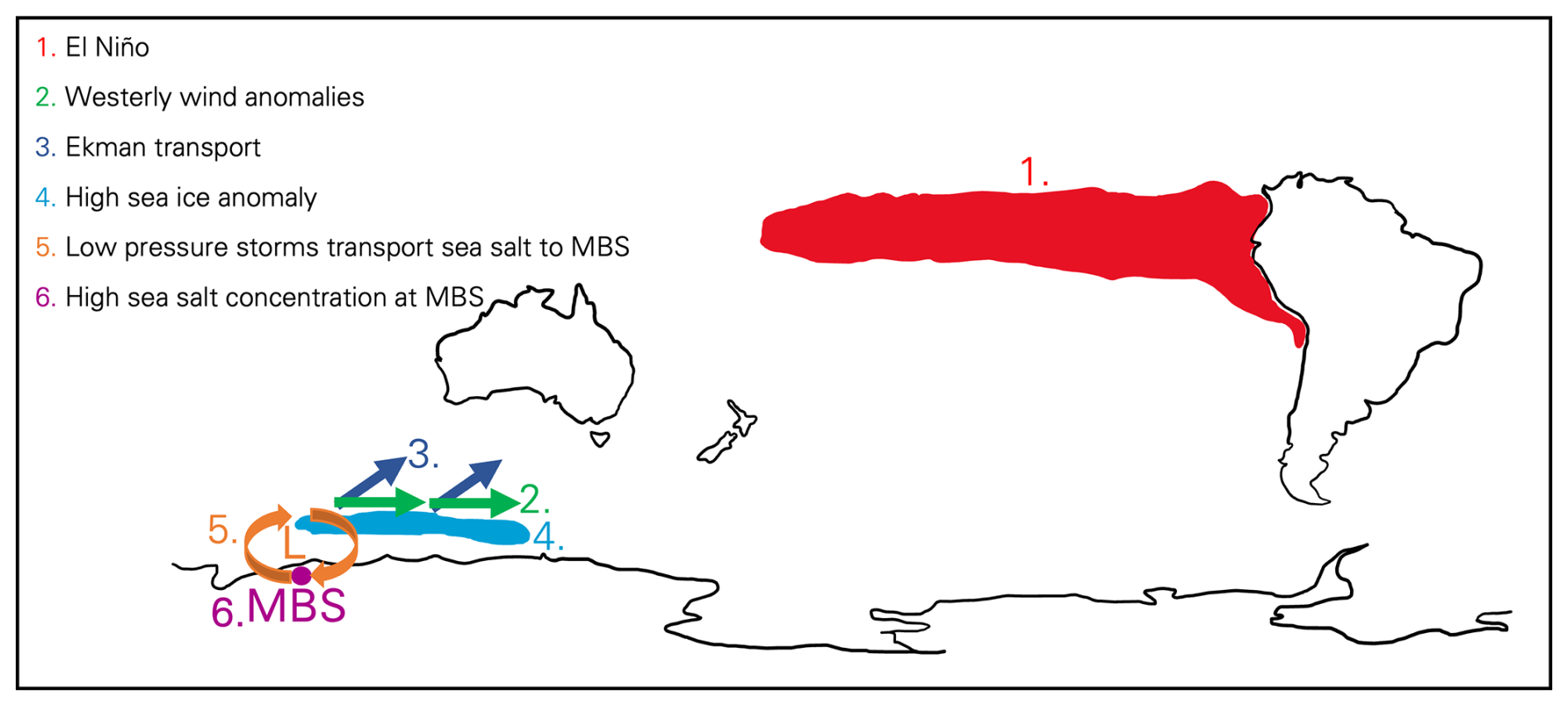
Figure 9 Schematic depicting the winter conditions associated with high sea salt concentration in the MBS ice core. Generated from composite maps (Figs. 2, 3, 5, 6).

The Law Dome ice core austral summer sea salt concentrations have a negative relationship with ENSO, with high sea salt concentrations associated with a La Niña signature (Vance et al., 2013; Crockart et al., 2021). This is in contrast with our schematic in Fig. 9, showing the region-specific influence of ENSO at MBS. Figure 9 was created using the annual sea salt concentrations from MBS, as opposed to just the austral summer sea salt concentrations used in the Law Dome analysis. The differences could be due to the different ice core locations and geographies and the wave like pattern of influence on sea ice from ENSO, as well as differences in the seasonal teleconnections of ENSO to Antarctica. Udy et al. (2022) found the November–February high sea salt concentrations in the Law Dome ice core to be associated with increased daily westerly wind anomalies which increase the amount of ocean spray producing sea salt aerosol. The schematic in Fig. 9 shows high sea salt concentration anomalies associated with austral winter averaged monthly westerly wind anomalies off the coast of MBS which is complementary with the findings from Udy et al. (2022). The fact that there are only two ice cores (MBS and Law Dome) in a large region of East Antarctica, and they have different relationships with ENSO highlights the need for more ice cores in the East Antarctic region, and also highlights the complexity of ENSO-Antarctic climate relationships (Macha et al., 2024).

A previous study of three high accumulation West Antarctic ice cores (76–78° S, 95–121° W) shows consistencies with the Fig. 9 schematic by suggesting the winter peak in sea salt concentrations are a result of sea ice in the region (Pasteris et al., 2014). An earlier study (Dixon et al., 2005) investigated the use of sea salts in West Antarctic ice cores, including International Trans-Antarctic Scientific Expedition (ITASE) cores, and demonstrated that factors contributing to the amount of sea salt aerosols transported inland include SIE, the presence of open-water, wind strength and direction, and the strength and positioning of low-pressure systems (Kaspari et al., 2005). This is in agreement with our analysis that SIE and low-pressure systems are important for sea salt aerosols reaching MBS (Fig. 9). Li et al. (2015) was able to reconstruct the sea ice extent in the Ross Sea in early austral winter through sea salt concentration in an interior East Antarctic ice core. They concluded that ENSO influenced the sea ice in the Ross Sea region, and through the transport of sea salt inland, influenced the sea salt deposition at the ice core site. These findings are comparable with our Fig. 9 schematic.

4.1 Limitations

We provide evidence on a possible mechanism for the delivery of sea salt to the MBS ice core. However, the mechanism is established through evidence from a short observational record, and the relationship with ENSO is based on only 10 El Niño-like and 10 La Niña-like years over the 38-year period. Therefore, it is difficult to separate the influence of ENSO to MBS with internal variability unrelated to the tropical Pacific in our analysis. Furthermore, our analysis only looks at the austral winter season. While we also consider circulation anomalies during spring, which we find to be weaker than in winter, it is possible that our winter-focus may be missing other seasonal mechanisms and relationships. Another limitation is around the definition of ENSO that we use – The important connection between the tropical Pacific and Antarctica is through the PSA pressure anomaly pattern, which may differ depending on the definition of ENSO upper and lower quartile years. Although ENSO diversity was not explicitly considered here, Table 1 shows that the traditional Niño3.4 region had the strongest correlations with MBS sea salts. However, the teleconnection to Antarctica also varies between Central and Eastern Pacific El Niño events (Wilson et al., 2014; Macha et al., 2024), which is not considered in our study.

Finally, we need to acknowledge that the results of this study show statistical relationships (often weak) of connections between fields, rather than definitive mechanistic pathways influencing the modulation of sea salt concentration in the MBS ice core. Therefore, these results should be considered as insights only. The MSLP composite maps show a potential extension of the PSA towards East Antarctica however the actual mechanism of the Rossby wave propagation from the tropical Pacific was not robustly investigated around the MBS region, as internal variability in circulation patterns overwhelms any coherent signal in the observational data. One avenue that might better interrogate the transport mechanism behind sea salt arriving at the MBS site is back trajectories. However, due to time limitations this was not undertaken in this study (also see Sect. 3.1).

4.2 Implications

The connection between sea salt concentration at MBS and SIC off the coast of MBS, with possible linkages to newly formed sea ice, is an important insight for using the long ice core record of MBS sea salt as a possible proxy for sea ice. Sea ice is a crucial part of the climate system influencing the surface albedo and interacting with the atmosphere and ocean exchange of heat, moisture, and trace gases such as CO₂ (Abram et al., 2013). Regular observations of sea ice began when satellites started collecting data in 1979. Due to this limited sea ice time series, it is difficult to understand how the sensitivity and dynamics of sea ice interacts with the climate system on longer time scales. There is no sea ice observational data for sea ice thickness or age that is useful for recording sea ice formation. Being able to use a climate proxy such as sea salt concentration in ice cores to interpret the low frequency variations in sea ice, in addition to sea ice formation, would be an invaluable resource to look far back in time before observations, and would complement existing ice-core-based reconstructions (Thomas et al., 2019) and station-based sea ice reconstructions (Fogt et al., 2022) of sea ice extent. This would allow longer–term context to be put on the recent, rapid decline in sea ice (Purich and Doddridge, 2023). For example, Li et al. (2015) used the sea salt concentrations from a 2680 year East Antarctic ice core (79° S, 77° E) as a proxy for sea ice extent in the Ross Sea, finding a significant ENSO influence. Our study suggests the MBS sea salt concentrations have the potential to provide a new sea ice proxy record for the last millennium from the full 1,137 year record. However, we also recommend a deeper examination of the sea ice–sea salt relationship and its causal mechanisms before such an attempt is made.

5 Conclusions

This study aimed to understand the mechanisms modulating the sea salt concentration variability at MBS in East Antarctica, and insights into the relationship with ENSO. We showed a relationship between the SIC near the MBS core location, and sea salt from the MBS ice core. Namely, high sea salt years corresponded to enhanced westerly winds and high SIC off the northeast coast of the MBS site. Our findings further suggest synoptic-scale storms off the coast of MBS are a possible key transport mechanism for sea salts from this area of sea ice to MBS. Moving from local processes to the large scale, the previously identified relationship between MBS sea salt concentration and ENSO (Crockart et al., 2021) was confirmed here. Our analysis suggests that El Niño events influence local processes around MBS through the generation of Rossby waves via the Pacific South America pattern. The influence of the PSA extends eastward around western Antarctica towards MBS, creating wind anomalies that impact both the formation of sea ice and sea salt aerosol from ocean spray. However, the teleconnection pathway between the PSA and localised circulation anomalies at the MBS site was unclear. Further, this teleconnection pathway appears non-linear, with connections only evident during El Niño, rather than La Niña events. This highlights the complexity of understanding the influence of ENSO on Antarctica in the past, and thus the difficulty in projecting how ENSO will interact with climate change to influence the continent in the future.

Appendix A

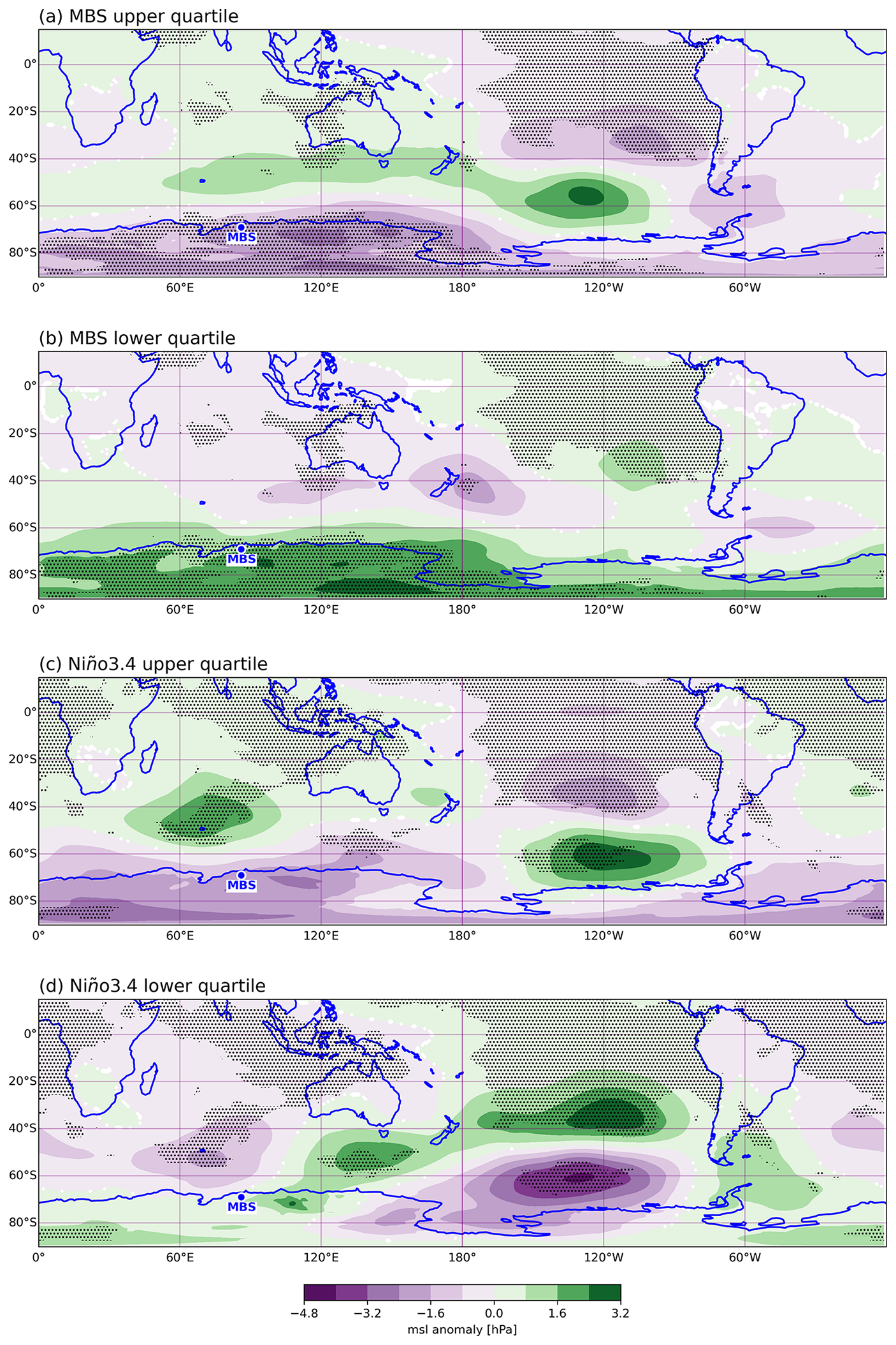
Figure A1 Composite maps of the winter ERA5 mean sea level pressure anomaly for the Mount Brown South site average (MBS Cl⁻) (a) upper [1982, 1986, 1987, 1993, 1996, 1997, 2009, 2012, 2014, 2015] and (b) lower quartile [1980, 1981, 1983, 1990, 1991, 1995, 1999, 2001, 2010, 2011] and for the Niño3.4 (c) upper [1982, 1987, 1991, 1993, 1997, 2002, 2004, 2009, 2012, 2015] and (d) lower quartile [1984, 1985, 1988, 1989, 1998, 1999, 2000, 2007, 2010, 2011]. The stippling indicates points where the mean sea level pressure anomaly K-S test p value is < 0.1. The blue dot indicates MBS.

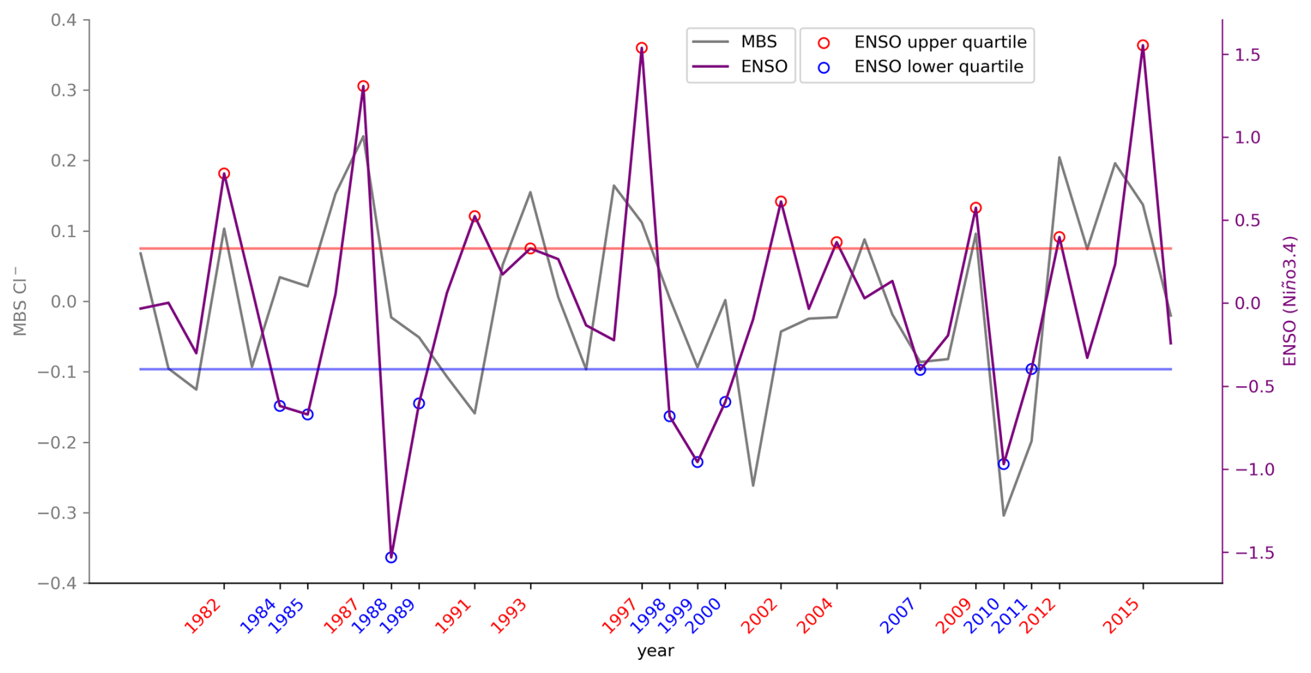
Figure A2 Time series of the annual detrended, log–transformed sea salt concentrations for the Mount Brown South site average (MBS Cl⁻) and the detrended (June–August) El Niño–Southern Oscillation region SST anomalies (Niño3.4). Red line (blue line) indicates the Niño3.4 upper (lower) quartile boundary. Red and blue years on the x axis represent the Niño3.4 upper and lower quartile years.

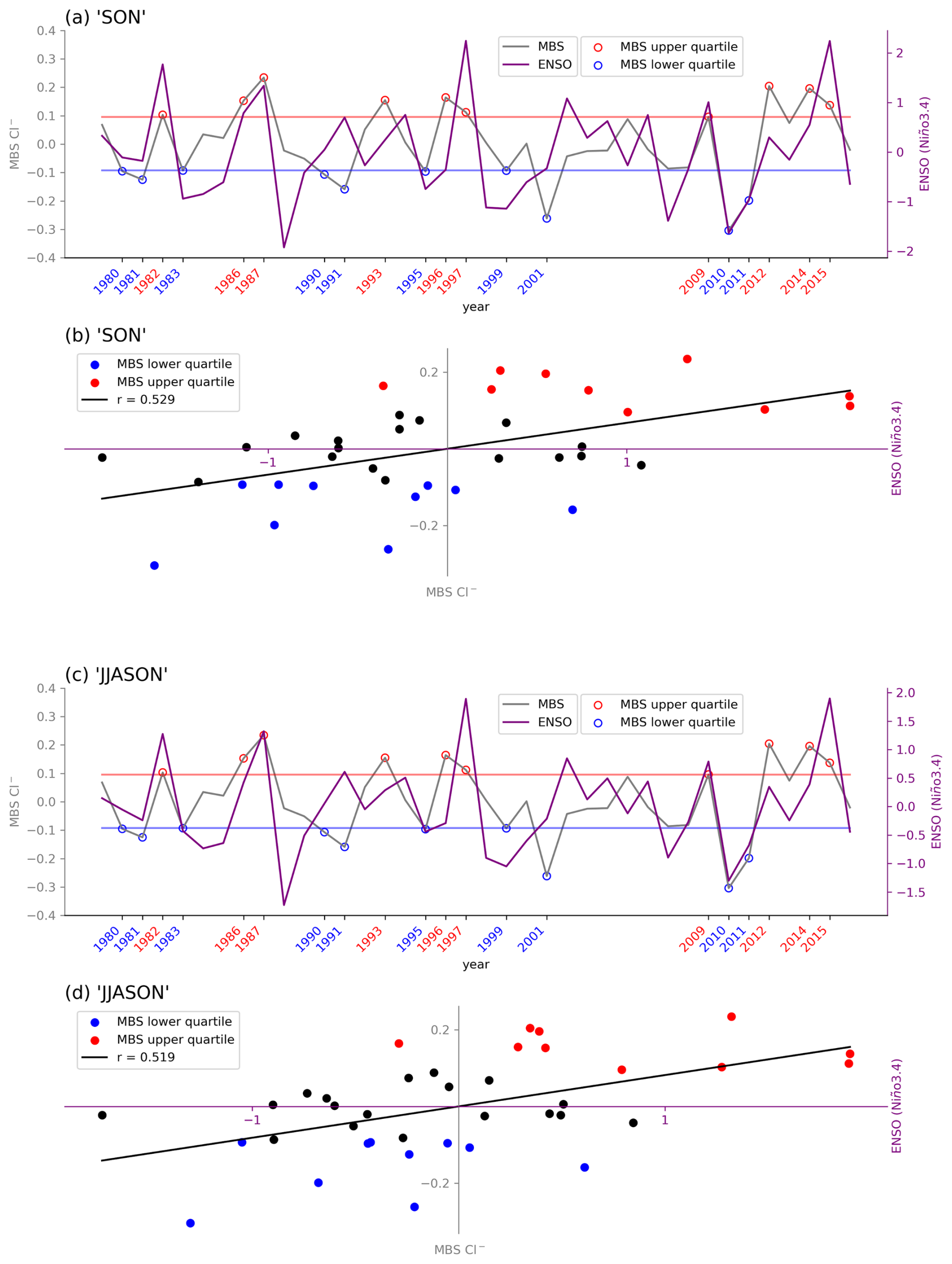
Figure A3 Time series of the annual detrended, log–transformed sea salt concentrations for the Mount Brown South site average (MBS Cl⁻) and the detrended (a) (September–November), (c) (July–November) El Niño–Southern Oscillation region SST anomalies (Niño3.4). Red line (blue line) indicates the upper (lower) quartile boundary. Scatter plot shows the relationship between the MBS Cl⁻ and (b) (September–November) Niño3.4 (d) (July–November) Niño3.4 with the MBS upper (lower) quartile highlighted by the red dots (blue dots) based on the period 1979–2016.

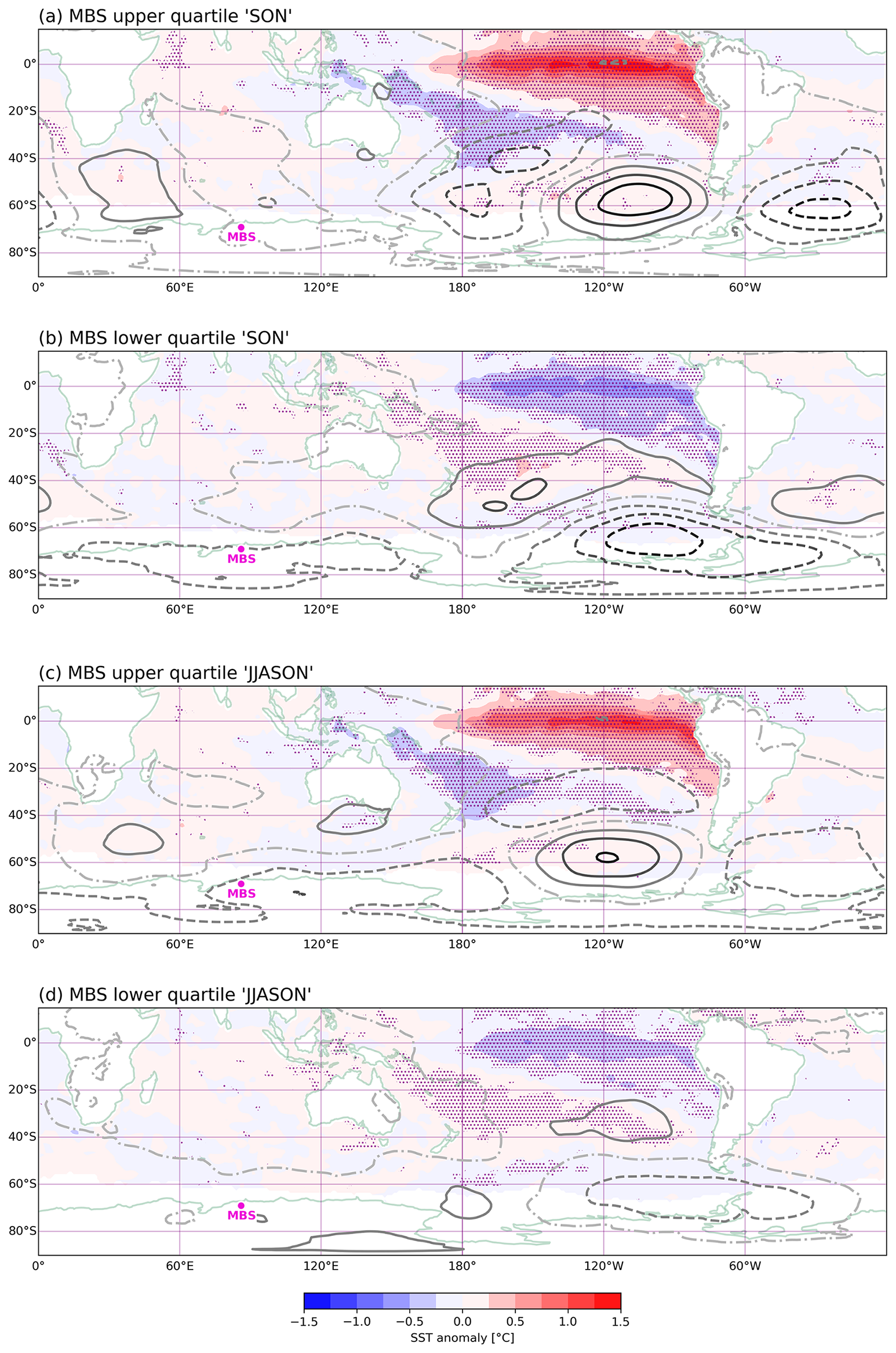
Figure A4 Composite maps of the (a, b) September–November, (c, d) July–November sea surface temperature anomaly (shading) and ERA5 mean sea level pressure anomaly (contours) for the Mount Brown South site average (MBS Cl⁻) (a, c) upper [1982, 1986, 1987, 1993, 1996, 1997, 2009, 2012, 2014, 2015] and (b, d) lower quartile [1980, 1981, 1983, 1990, 1991, 1995, 1999, 2001, 2010, 2011]. High (low) MSLP anomalies shown by solid (dashed) contours, with darker shades of grey indicating stronger anomalies. The contour line graduations indicate 0.8 hPa. The stippling indicates points where the sea surface temperature anomaly (shading) K-S test p value is < 0.1. The fuchsia dot indicates MBS.

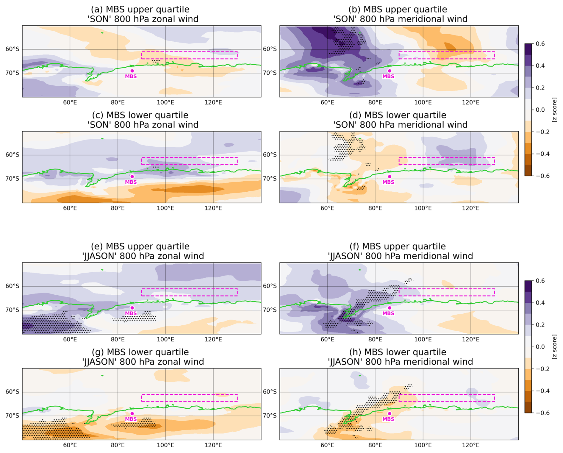
Figure A5 Composite maps of the (a–d) September–November, (e–h) July–November ERA5 800 hPa meridional and zonal wind anomalies for the Mount Brown South site average (MBS Cl⁻) (a, e) upper and (c, g) lower quartile of zonal wind and (b, f) upper and (d, h) lower quartile of meridional wind. Upper quartiles (a, b, e, f) [1982, 1986, 1987, 1993, 1996, 1997, 2009, 2012, 2014, 2015] and lower quartiles (c, d, g, h) [1980, 1981, 1983, 1990, 1991, 1995, 1999, 2001, 2010, 2011]. The stippling indicates points where the K-S test p value is < 0.1. The MBS northeast coast box is highlighted in fuchsia and the fuchsia dot indicates MBS.

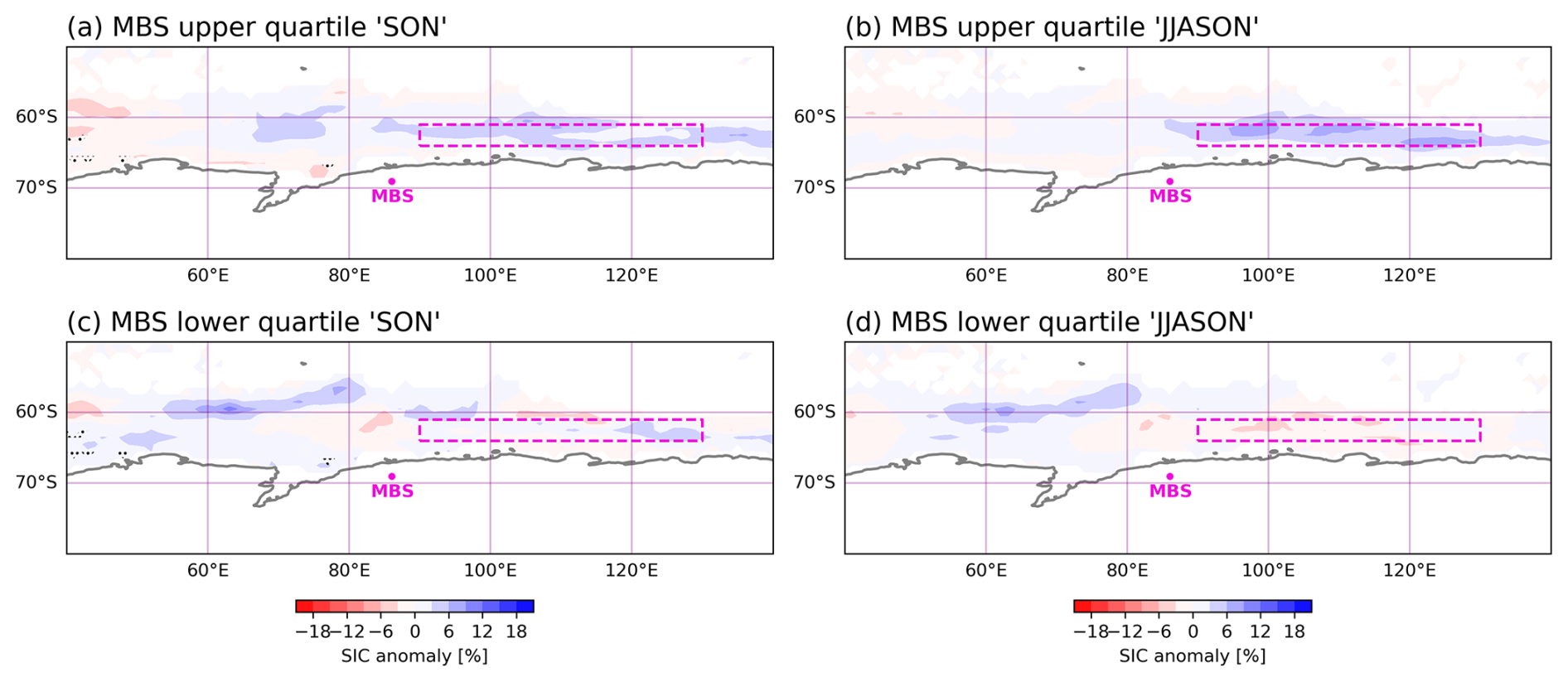
Figure A6 Composite maps of the (a, c) September–November, (b, d) July–November sea ice concentration for the Mount Brown South site average (MBS Cl⁻) (a, b) upper [1982, 1986, 1987, 1993, 1996, 1997, 2009, 2012, 2014, 2015] and (c, d) lower quartile [1980, 1981, 1983, 1990, 1991, 1995, 1999, 2001, 2010, 2011]. The stippling indicates points where the K-S test p value is < 0.1. The MBS northeast coast box (61–64° S, 90–130° E) highlighted by the fuchsia dashed line while the fuchsia dot indicates MBS.

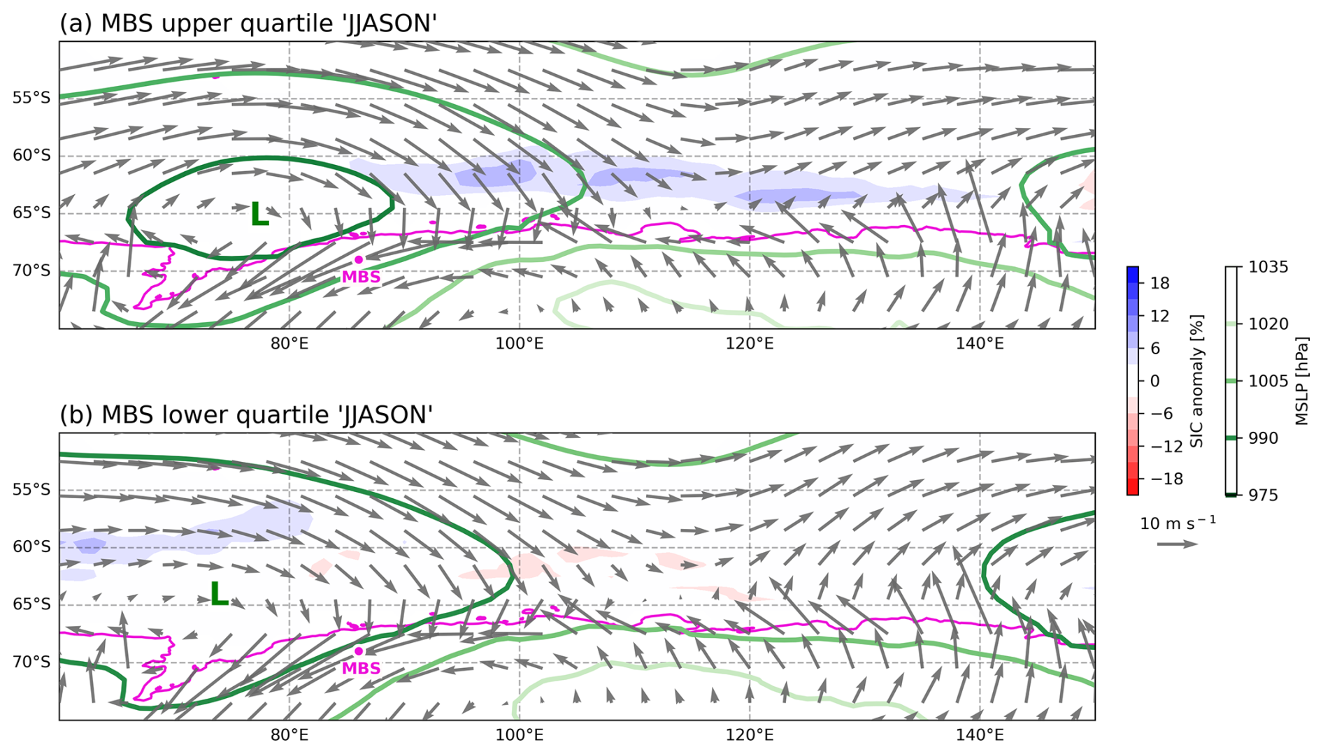
Figure A7 Composite maps of the daily ERA5 mean sea level pressure (contours), daily ERA5 800 hPa mean wind vectors averaged over the 5 maximum precipitation days in JJASON, JJASON averaged sea ice concentration (shading) for the Mount Brown South site average (MBS Cl⁻) (a) upper [1982, 1986, 1987, 1993, 1996, 1997, 2009, 2012, 2014, 2015] and (b) MBS lower quartile [1980, 1981, 1983, 1990, 1991, 1995, 1999, 2001, 2010, 2011]. The fuchsia dot indicates MBS.

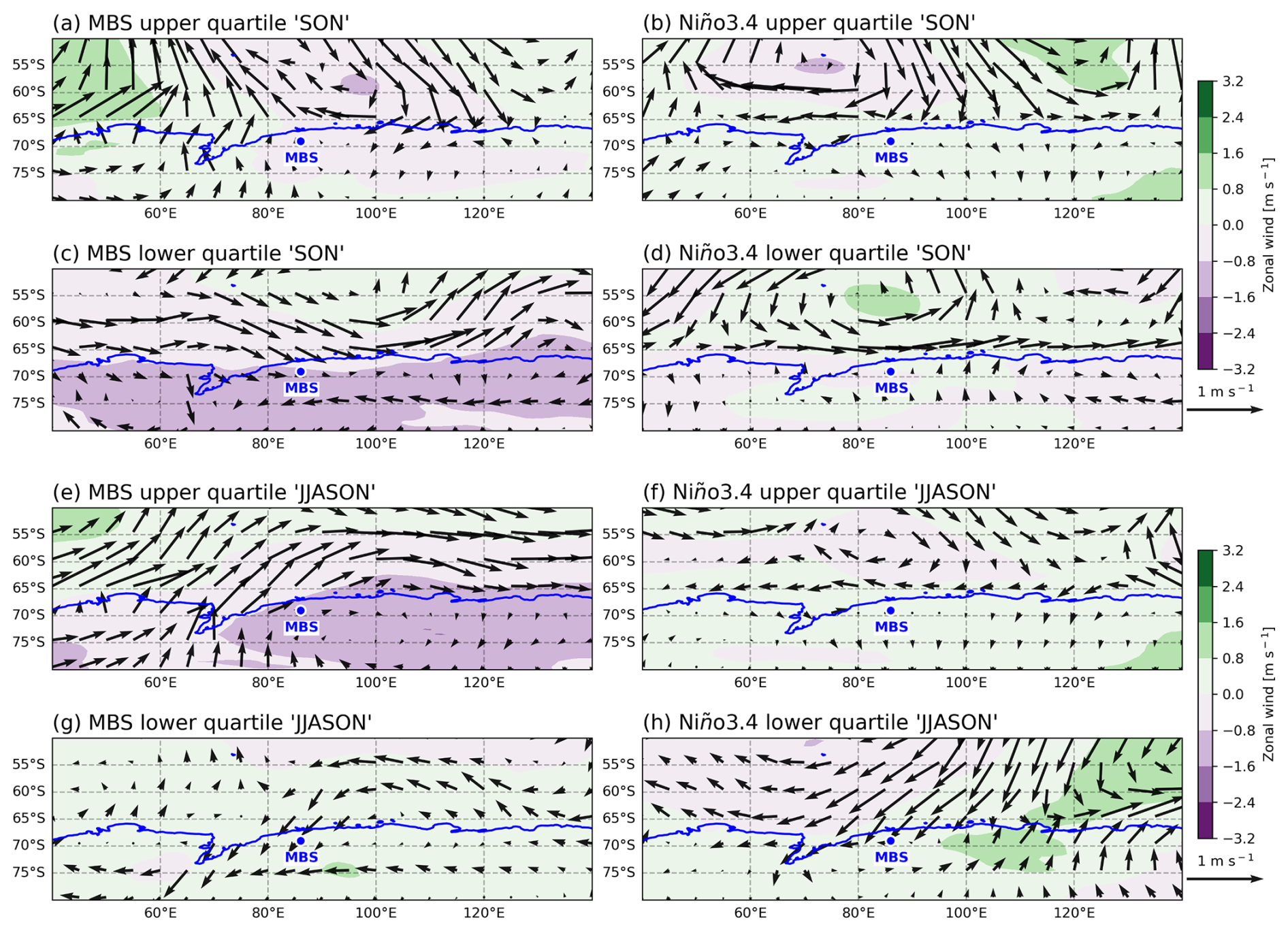
Figure A8 Composite maps of the (a–d) September–November, (e–h) July–November ERA5 mean sea level pressure anomaly (shading) with 800 hPa wind vector anomalies overlayed for the Mount Brown South site average (MBS Cl⁻) (a, e) upper [1982, 1986, 1987, 1993, 1996, 1997, 2009, 2012, 2014, 2015] and (c, g) lower quartile [1980, 1981, 1983, 1990, 1991, 1995, 1999, 2001, 2010, 2011] and the Niño3.4 (b, f) upper and (d, h) lower quartile.

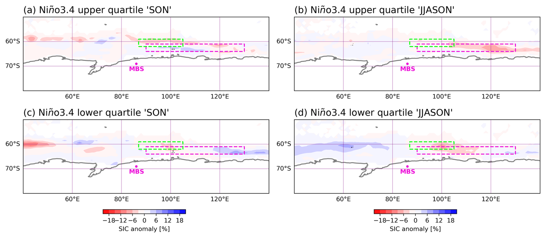
Figure A9 Composite maps of the (a, c) September–November (SON), (b, d) July–November (JJASON) sea ice concentration for the Niño3.4 (a) SON, (b) JJASON upper and (c) SON, (d) JJASON lower quartile. The stippling indicates points where the K-S test p value is < 0.1. The MBS northeast coast box (61–64° S, 90–130° E) highlighted by the fuchsia dashed line while the fuchsia dot indicates MBS.