Tropical temperature evolution across two glacial cycles derived from speleothem fluid inclusion microthermometry

The evolution of tropical temperature across multiple glacial-interglacial cycles is mostly constrained with marine proxy records, which are associated with considerable uncertainties. Here we present a reconstruction of tropical cave temperatures derived from fluid inclusions in stalagmite WR5_B from Whiterock Cave (Gunung Mulu National Park, Northern Borneo). The employed paleothermometer – nucleation-assisted microthermometry – is based on the density of the water trapped in fluid inclusions, i.e., on a well-known thermodynamic parameter and yields highly precise temperature estimates. The record consists of 49 temperature data points spanning a 127 kyr period from 460 to 333 ka including the glacial terminations T-V and T-IV. We find that Borneo temperature tracks Southern Hemisphere temperature and atmospheric CO₂ concentrations. Deglacial warming is accompanied by relatively dry conditions in Northern Borneo, indicated by pronounced enrichments in calcite δ¹⁸O_cc and reconstructed drip water δ¹⁸O_dw values. The amplitude of glacial-interglacial temperature changes amounts to 4.2 ± 0.4 °C (2 SEM) between MIS 12 and the MIS 11 interglacial optimum and 4.3 ± 0.4 °C (2 SEM) across T-IV. MIS 11 peak temperature was found to be 0.9 ± 0.4 °C warmer than late Holocene temperatures reconstructed for Whiterock Cave, whereas temperatures during MIS 12 and MIS 10 glacial maxima in our record are indistinguishable from those previously reconstructed for the Last Glacial Maximum. Both the present WR5_B record as well as the recently published record from Løland et al. (2022) covering the last glacial Termination exhibit a clear linear correlation with Antarctic temperature anomalies (R²=0.89 and 0.97, respectively), with practically identical slopes of the linear regression lines. Depending on the employed Antarctic ΔT reconstruction, Landais et al. (2021) and Jouzel et al. (2007), we found a site-specific polar (Antarctic) amplification factor of 2.21 ± 0.22 and 2.42 ± 0.23 (95 % CI), respectively.

1 Introduction

The glacial-interglacial cycles of the Pleistocene offer valuable opportunities to study the response of the global climate system to varying boundary conditions such as atmospheric CO₂ concentration, and to identify the processes that characterize large global climate shifts between glacial and interglacial states. The larger glacial-interglacial cycles of the last million years feature many similarities, but also clear differences, especially in the magnitude, duration, and temporal evolution of the interglacials (Past Interglacial Working Group of PAGES, 2016). Improved constraints as to how these interglacials differed in terms of global and regional characteristics will yield important insights into the interactions and sensitivities of the different climate system components.

Quantitative temperature reconstructions are crucial to assessing the global and regional sensitivity to varying greenhouse forcing and furthermore serve as important benchmarks for earth system models. However, apart from the detailed temperature reconstructions from Antarctic ice cores (Jouzel et al., 2007; Landais et al., 2021), the vast majority of glacial-interglacial temperature reconstructions come from marine sediments for long-term temperature records with scant records derived from land. Marine temperature proxies are associated with uncertainties regarding the water depth and seasonality of the signal production (Ho and Laepple, 2016; Bova et al., 2021) and are often affected by additional, non-thermal factors such as salinity, pH and biological effects (e.g., Gray and Evans, 2019). Discrepancies between proxy-based temperature reconstructions underly a long-standing debate on the amplitude of glacial-interglacial temperature changes in the tropics (see an overview in Tripati et al., 2014).

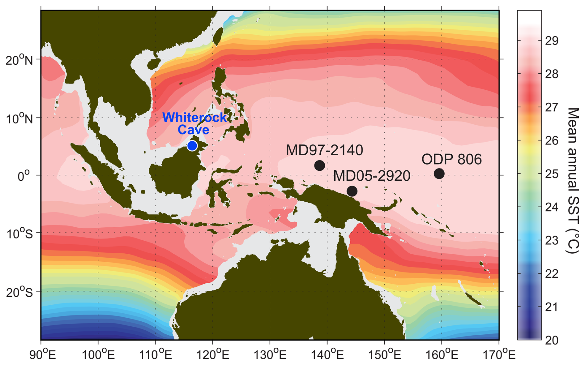
Figure 1 Map of modern-day mean annual sea surface temperatures (SST) in the Western Pacific Warm Pool region. Shelf areas that were exposed during glacial sea level lowstands (−120 m) are shown in white. The locations of Whiterock Cave (Gunung Mulu National Park, Northern Borneo) as well as three marine core sites with SST reconstructions relevant to this study (see Sect. 4.2) are indicated with dots. Modified after Meckler et al. (2012, Supplement).

The advancement of several quantitative proxy methods for speleothem-based temperature reconstructions such as δ¹⁸O thermometry based on fluid inclusion and calcite oxygen isotopic compositions (e.g. Affolter et al., 2014), noble gas thermometry (e.g. Kluge et al., 2008), clumped isotope thermometry (e.g. Affek et al., 2008) or TEX86 (e.g. Baker et al., 2019) opens new opportunities to fill in the gap of terrestrial temperature data by producing quantitative records from different karst areas around the globe. Here we employ what is arguably the most precise and accurate of these methods (cf. Meckler et al., 2015), nucleation-assisted (NA) microthermometry, which is based on fluid inclusion liquid-vapour homogenisation (Krüger et al., 2011). The main advantages of this paleothermometer are its physical basis (circumventing the need for empirical calibration) and its high precision (typical 2σ standard errors of the mean (2 SEM) are around 0.3 °C).

Here, we applied NA microthermometry to a stalagmite from Northern Borneo, located in the heart of the Western Pacific Warm Pool (Fig. 1). Stalagmite WR5_B covers almost two glacial-interglacial cycles from Marine Isotope Stage (MIS) 12 to MIS 9, including two glacial terminations, T-V (also known as Mid-Brunhes transition) and T-IV, as well as the glacial inception from MIS 11 to MIS 10. MIS 11 is an unusually long and warm interglacial period (Tzedakis et al., 2022; Past Interglacial Working Group of PAGES, 2016) that, like the Holocene, is characterised by relatively weak insolation forcing, i.e., a small amplitude of the precession cycle due to the low eccentricity of the Earth's orbit. Using the same analytical method, Løland et al. (2022) presented a temperature reconstruction across the last glacial termination showing that Borneo land temperature closely tracks the deglacial evolution of atmospheric CO₂ and Antarctic temperature and is largely decoupled from hydroclimate changes that are strongly impacted by Northern Hemisphere cooling events. Here we investigate whether the same holds true also for earlier glacial terminations and across glacial-interglacial cycles and we assess the amplitude of glacial interglacial temperature changes. Given that this paleothermometer is not yet widely established, we include a detailed description of the method and discuss uncertainties related to measurements and the resulting cave temperature reconstructions in Sect. 2.

2 Materials and Methods

2.1 Temperature monitoring

Stalagmite WR5 was collected in 2008 from Whiterock Cave (Gunung Mulu National Park, Northern Borneo, Malaysia; 4.1° N, 114.9° E) in a cave chamber about 350 m from “Midnight Entrance” (180 m a.s.l.). The depth of the site below surface is estimated at about 100 m and present-day air temperature in the cave chamber is 23.7 °C. Continuous temperature monitoring close to the location of WR5 over a 30 month period, from March 2018 until September 2020, revealed minor fluctuations of the cave air temperature of about ± 0.1 °C (total amplitude), indicating very stable temperature conditions throughout the year. For comparison, temperatures recorded at the cave entrance during the same period show daily and seasonal fluctuations and a average air temperature of 25.1 °C over a full 2-year cicle (July 2018–June 2020), which is 1.4 °C higher than the temperature recorded inside the cave. Surface air temperatures measured at two locations in Gunung Mulu National Park (at ca. 30 m a.s.l.) over the same 24 months period yield average temperatures of 25.5 (rainforest) and 26.6 °C (open clearing). These temperatures are consistent with the temperature at the cave entrance when allowing for the 150 m altitude difference with a lapse rate of 0.6 °C/100 m (Løland et al., 2022). ERA5-T2m reanalyisis land temperatures (KNMI Climate Explorer, 2025) of the nearby lowland area at 3.85–4.25° N, 114.60–114.85° E for the same period yield an average temperature of 26.7 °C, which is in agreement with our monitoring data of outside air temperatures (Fig. A1; see Appendix). We note that previously reported temperature data recorded between 2006 and 2012 at the nearby meteorological station at Mulu airport (24 m a.s.l.), in contrast, indicate significantly lower surface air temperatures, averaging at 24.3 °C over the entire 6-year period with annual mean temperatures varying between 24.0 and 24.7 °C. The respective ERA5-T2m average temperature over this period is 26.1 °C. Although the altitude-corrected 6-year average temperature from Mulu airport (23.4 °C) is close to the measured cave temperature and matches even better when considering a regional warming trend of about 0.3 °C/decade (based on reanalysis data), the airport temperature data are in clear contradiction with the other temperature records, and we therefore consider them as not representative for the area.

The observed deviation between cave and outside air temperature (as measured at the cave entrance) means that the assumption of identity of cave and (coeval) surface air temperature is not applicable to Whiterock Cave, and that their relationship is more complex. Although it is generally accepted that cave temperature is controlled by surface temperature, theoretical studies have demonstrated that the transfer of the temperature signal into the cave involves a systematic lag of the cave temperature in response to changes of outside surface air temperature: The heat flux into the cave is governed by different physical processes including heat conduction through the overlaying karst bedrock (Dominguez-Villar et al., 2020), convective heat transport by water infiltration (Badino, 2004, 2010) and advective heat transport related to air flow through the cave galleries (Luetscher and Jeannin, 2004). The relative contribution of these processes controls the heat flux, and thus, the lag time of the cave temperature relative to the outside temperature signal and is cave-specific, depending on the geometry and climatic setting of the cave. The delay of the signal transfer acts as a low-pass filter resulting in a potential attenuation of the amplitude of outside temperature anomalies in the cave (Dominguez-Villar et al., 2020). This is most obvious on daily and seasonal time scales but depending on the actual lag or equilibration time of the system, attenuation of the outside temperature signal may also occur on decadal, centennial or even longer time scales.

In a tropical setting like Northern Borneo with high annual precipitation of 4000–5000 mm m⁻², convective heat transport through fracture flow of infiltrating water is likely dominating the heat flux into the cave. Badino (2010) pointed out that the infiltrating rainwater is typically colder than mean surface air temperature and may decrease the cave temperature below outside air temperature, thus resulting in a systematic offset. If this holds true for Whiterock Cave, it would be an additional factor contributing to the observed temperature difference between cave and surface air. Given a rapid warming in the region by about 1.5 °C since the late 1960's according to the reanalysis data, a deviation of the cave temperature from outside air temperature is therefore not surprising but is to be expected.

How does this affect the interpretation of the cave temperature record? The amplitude of a change in cave temperature can generally be considered as a minimum estimate of the actual amplitude of the surface air temperature signal. The lower the frequency, i.e. the longer the duration of the temperature anomaly relative to the signal delay, the closer the cave temperature approaches the amplitude of the surface signal. In the present study we are dealing with cave temperature changes on millennial and orbital time scales and considering the climatic setting and depth of the cave below surface, we assume that the amplitude of the reconstructed temperature changes in Whiterock Cave closely reflects the amplitude of the outside temperature signal. We will get back to this in Sect. 5.

2.2 Stalagmite sample

WR5 is a fossil stalagmite with a total length of 400 mm that was found tipped over on a rock pile. For the present study, we used the lower ca. 190 mm long section of the stalagmite denoted as WR5_B (Fig. 2) that covers a 127 kyr time interval from 460 to 333 ka, and thus, includes two glacial terminations (T-V and T-IV). WR5_B has previously been studied with regard to tropical hydroclimate using the oxygen isotope signal of the calcite, δ¹⁸O_cc (Meckler et al., 2012), and later on, was employed for a comparison study of different speleothem paleo-thermometers (Meckler et al., 2015).

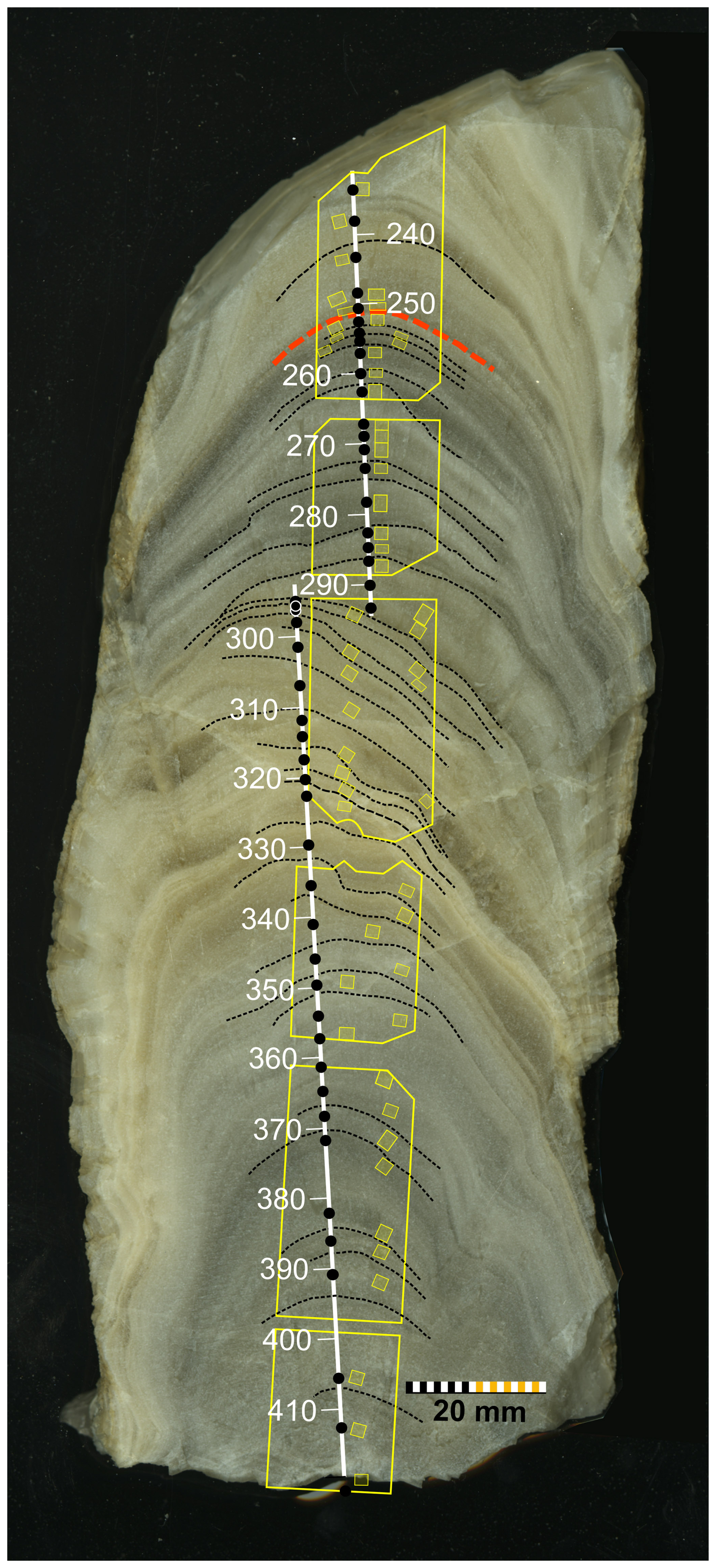
Figure 2 Cross section of stalagmite WR5_B sub-parallel to the central growth axis. White lines with millimetre gradations indicate the location of the calcite isotope transect. Yellow polygons show the outlines of the sample blocks from which the thick sections for petrographic and fluid inclusion analysis were cut and their position with respect to the isotope transect. Yellow shaded squares label the 49 sample positions at which fluid inclusions were analysed for this study. Black dots represent the respective sample positions on the isotope transect. Dotted lines indicate growth hiatuses. Note, the red dotted line marks a major hiatus at the beginning of Termination IV (see Figs. A2a and h, 3, and 6b–d).

The stalagmite exhibits distinct colour changes that can be assigned to glacial (grey) and interglacial (yellow ochre) periods. The calcite fabric that was analysed on 200 µm thick polished stalagmite sections is predominantly columnar open (Frisia, 2015) showing large, up to cm-wide composite crystals that are build up from columnar crystal units of almost perfectly uniform c-axis orientation (Fig. A2a, b; see Appendix). Fluid inclusions of appropriate size (10³–10⁵ µm³) are abundant and of primary origin, i.e. they formed during crystal growth by incomplete lateral coalescence of adjacent columnar crystal units (cf. Kendall and Broughton, 1978). The uniform c-axis orientation of the columnar crystal units is likely to promote a tight sealing of the predominantly inter-crystalline inclusions. Characteristically, the inclusions are monophase liquid and exhibit elongate spindle-like shapes with a thorn-shaped tip at the upper end (Fig. A2c, d). Occasionally, two-phase inclusions are also present, but these were ignored because their bulk water densities are not related to stalagmite formation temperatures. They likely result from leakage or stretching of the inclusions, which at some point provokes a spontaneous nucleation of the vapour bubble.

Petrographic inspections of the thick sections allowed for identifying more than 30 potential growth interruptions in WR5_B. Some of these hiatuses display irregular surface structures (Fig. A2e) likely resulting from calcite dissolution (Type E surfaces; Railsback et al., 2013), whereas others exhibit smooth surfaces marked by numerous tiny fluid inclusions (Fig. A2f). After a hiatus, crystal growth generally continued with the same crystallographic orientation. In one case (at position 320 mm), however, small, potentially detrital calcite crystals of random crystallographic orientation can be observed on the hiatus surface (Fig. A2g). Subsequently, they were overgrown by the columnar calcite fabric due to geometric selection and competitive growth (Kendall and Broughton, 1978).

In addition to WR5_B we analysed a 35 mm long drill core sample (WR_MC1) from an actively growing stalagmite that was collected only a few meters away from WR5_B. WR_MC1 features a calcite fabric similar to that of WR5_B (Fig. A5). The bottom age of the drill core sample was dated at 3.45 ± 0.25 ka allowing us to reconstruct a late Holocene reference temperature for Whiterock cave that can be directly compared to temperatures derived from WR5_B.

2.3 Age model

U/Th dating of stalagmite WR5_B has previously been conducted by Meckler et al. (2012). The dating, however, was impaired by very low Uranium concentrations and several age reversals. Due to these difficulties, the initial age model of WR5_B was finally obtained by aligning the δ¹⁸O_cc record of WR5_B with a refence record obtained from another, better dated Borneo stalagmite (GC08) that exhibits a very similar pattern of the δ¹⁸O_cc signal. Stalagmite GC08 covers the time interval from 570 to 210 ka and originates from Green Cathedral Cave in Gunung Buda, located about 10 km northeast of Whiterock Cave. Although GC08 contains significantly more Uranium, the initial δ²³⁴U ratios were very low (−613 ‰ on average) and had to be assumed constant in order to derive a robust age model (Meckler et al., 2012). Resulting errors of the GC08 age model are therefore relatively large, on the order of ± 12 kyr, for the time interval covered by WR5_B.

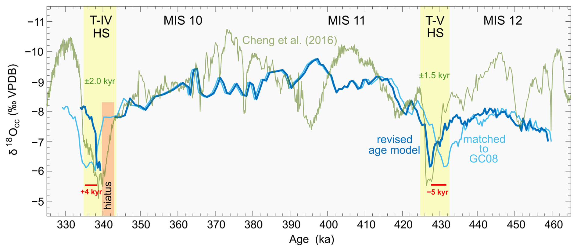
Figure 3 Revision of the WR5_B age model using the calcite δ¹⁸O record. Light blue: The original WR5_B age model (Meckler et al., 2012) was obtained by matching the δ¹⁸O_cc record to the one from stalagmite GC08 (not shown). Green: Chinese Monsoon record (Cheng et al., 2016) showing pronounced δ¹⁸O_cc excursions related to Heinrich events during T-V and T-IV. Age errors of the monsoon record are about ± 1.5 and ± 2.0 kyr for the time intervals around T-V and T-IV, respectively. Blue: revised WR5_B age model featuring a 3 kyr hiatus at the beginning of T-IV (see Fig. 2). The revised model shifts the original ages around T-V and T-IV by ca. −5 and +4 kyr, respectively. Note the reversed y-axis.

The δ¹⁸O_cc records from both Borneo stalagmites display distinct maxima at glacial terminations T-V and T-IV that have been interpreted as deglacial drying phases (Meckler et al., 2012). Similar maxima of the δ¹⁸O_cc signal also occur in the Asian Monsoon record (Cheng et al., 2016) that is based on well dated stalagmites from Sanbao Cave (central China) with dating errors of about ± 2.5 kyr at T-IV and ±1.5 kyr at T-V. Other Borneo stalagmites with better chronological constraints spanning the last glacial termination (T-I) show that the deglacial maximum in δ¹⁸O_cc occurs simultaneously in the Chinese monsoon record and coincides with North Atlantic cooling during Heinrich stadial 1 (HS-1; Partin et al., 2007). Assuming the same synchronicity of the δ¹⁸O_cc maxima in the monsoon and Borneo records during the older deglaciations covered by WR5_B, we used the more accurate and precise age model of the Sanbao Cave stalagmites to improve the age model of WR5_B for the T-IV and T-V Heinrich stadials. The result is a shift of the initial WR5_B ages by about +4 kyr at T-IV and by −5 kyr at T-V shown in Fig. 3. At Termination IV, the new age model additionally discloses a major hiatus (red dashed line in Fig. 2) that stands out by a clear discontinuity in the isotope δ¹⁸O_cc record. Based on our match to the monsoon record, we estimate the duration of this growth interruption to about 3 kyr. We emphasise that these adjustments of the WR5_B age model were restricted to the Heinrich stadials only, while ages during MIS12, MIS 11 and MIS 10 remain unaltered, and thus, are associated with relatively large age errors, including uncertainties arising from hiatuses of unknown duration. Moreover, a low average growth rate of 2.1 µm yr⁻¹ limits the achievable temporal resolution of the WR5_B cave temperature record.

2.4 Fluid inclusion ages

To ascertain the ages of the fluid inclusions, the position of the analysed samples relative to the δ¹⁸O_cc reference profile was determined by visual correlation of prominent growth bands using high-resolution images of the thick sections and of the polished cut face of the stalagmite half on which the isotope transect had previously been drilled. While inclusion-rich layers appear brighter than inclusion-poor layers in reflected light on the (non-translucent) stalagmite half (Fig. 2), they appear darker in the translucent ca. 200 µm thick petrographic sections viewed in transmitted light (see Figs. A2, A5). To avoid potential confusion, we used an inverted grey-scale image of the stalagmite half (not shown) and compared it with the conventional grey-scale images of the thick sections. Maximum errors of the visual layer correlation are estimated at ±1 mm. The ages of the individual samples were then determined based on the revised age model of WR5_B (Sect. 2.3). At each sample position, fluid inclusions were analysed within a narrow band of 1–3 mm width in axial (growth) direction of the stalagmite. Depending on the width of these bands and the stalagmite growth rate, the estimated maximum time intervals covered by a sample range between 0.2 and 3.0 kyr (see Table 1). However, since the age model and inferred growth rates do not take account of unresolved growth interruptions some of these time intervals might be significantly shorter.

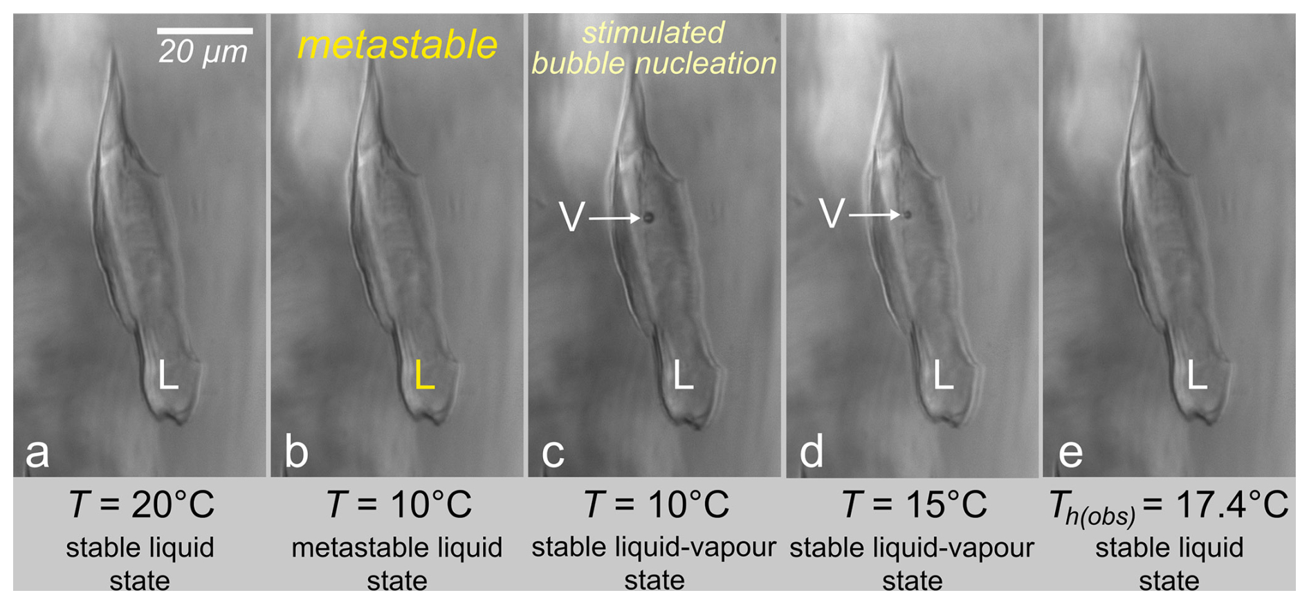
Figure 4 Image sequence illustrating the different states (a–e) of a WR5_B fluid inclusion during microthermometric measurements. After transferring the inclusion from a stable into a metastable liquid state (from a to b), a single ultra-short laser pulse is applied to stimulate vapour bubble nucleation (c). Subsequently, the inclusion is heated, and the bubble becomes progressively smaller (d) until it collapses at T_h(obs) (e), where the inclusion homogenizes into a stable liquid state. Modified after Krüger et al. (2014).

2.5 Fluid inclusion liquid-vapour homogenisation

Fluid inclusions in speleothems contain relicts of former drip waters from which calcite precipitated. The density ϱ of the enclosed water is assumed to relate directly to the cave temperature at the time the inclusions sealed off from the environment, and thus, can be used as a quantitative proxy to determine stalagmite formation temperatures T_f, i.e., cave temperatures (Krüger et al., 2011; Løland et al., 2022). The density of the water in the inclusions can be deduced from measurements of the liquid-vapour homogenisation temperature T_h, using nucleation-assisted (NA) fluid inclusion microthermometry. Prior to measuring T_h, however, the initially monophase inclusions must be cooled below their expected homogenisation temperature and then transferred from a metastable liquid to a stable liquid-vapour equilibrium state. To do so, we apply single ultra-short laser pulses to stimulate vapour bubble nucleation (Krüger et al., 2007), thus overcoming the long-lived metastability of the liquid state that prevents spontaneous bubble nucleation. Upon subsequent heating, the liquid phase expands at the expense of the vapour bubble that becomes continuously smaller. Eventually, the vapour bubble collapses, and the inclusion homogenises to a stable liquid state. This temperature is referred to as observed homogenisation temperature T_h(obs). Figure 4 displays an image sequence illustrating the different stages of a fluid inclusion during microthermometric analysis.

2.6 Nucleation-assisted microthermometry

Microthermometric analyses were performed with a Linkam THMSG600 heating/cooling stage. The stage is mounted on an Olympus BX53 microscope equipped with an Olympus LMPLFLN $\mathrm{100}\times /\mathrm{0.8}$ long working distance objective and a digital camera (pco.edge 3.1) for visual observation of the inclusions in transmitted light. Synthetic H₂O and H₂O-CO₂ fluid inclusion standards are used for temperature calibration, yielding an accuracy of the heating/cooling stage of ± 0.1 °C. Reference temperatures are the triple point of water (0.0 °C) and the critical point of CO₂ (31.4 °C in the H₂O-CO₂ system; Morrison, 1981).

For the microthermometric measurements we prepared separate, 200–300 µm thick unpolished sections that were removed from the glass slides after cutting, and finally, split into fragments of about 5 mm in size that fit on the sample holder of the Linkam stage. In order to make these samples transparent for microscopic observation of the fluid inclusions, they are coated on both sides with a thin film of immersion oil to reduce light scattering at the raw cut faces.

Depending on the inclusion size, the samples were cooled 4 to 10 °C below the expected homogenisation temperature prior to stimulating vapour bubble nucleation by means of ultra-short laser pulses provided by an amplified Ti:Sapphire femtosecond laser system (CPA-2101, Clark-MXR, Inc.). The laser with a centre wavelength of 775 nm and a nominal pulse width of <150 fs is operated in single pulse mode, releasing a single laser pulse at the push of a trigger button. The pulse energy is attenuated in three steps by approximately a factor of 50 000 before the laser beam is coupled into the microscope via a short-pass dichroic beam splitter and focused on the fluid inclusion through the 100× objective. The last attenuation step, consisting of a rotatable halfwave plate and a fixed Glan laser polarizer, allows for the fine-tuning of the pulse intensity of the focused laser beam to a level that is at or slightly above the threshold for vapour bubble nucleation but below the threshold for visible calcite ablation (Krüger et al., 2007). This is essential to avoid damaging of the inclusions and thereby altering their volume properties. A schematic representation of the analytical setup is shown in Fig. A3. The setup allows us to repeatedly induce vapour bubble nucleation in pre-selected fluid inclusions under simultaneous visual observation and to perform subsequent measurements of T_h(obs) without moving the sample.

2.7 Analytical precision

At least two replicate measurements of T_h(obs) were performed for each inclusion, yielding a typical reproducibility (precision) within ± 0.05 °C. Inclusions that did not homogenize below a certain threshold temperature (between 25–28 °C depending on the climatic period) were rejected since they were likely subject to density alteration due to stretching or partial leakage. Upper limits for T_h(obs) measurements are used as a precaution to avoid potential stretching of other inclusions in the sample caused by high internal fluid pressure that builds up when the inclusions are heated far above T_h(obs).

As T_h(obs) depends not only on the density of the enclosed water but also on the volume of the inclusions, we applied a correction to compensate for the effect of surface tension on liquid-vapour homogenisation (Fall et al., 2009). Based on T_h(obs) and additional measurements of the vapour bubble radius r(T) derived from bubble images taken at known temperature, we calculated the homogenisation temperature T_h∞ of a hypothetical, infinitely large fluid inclusion using the thermodynamic model proposed by Marti et al. (2012). The model is based on the IAPWS-95 formulation (Wagner and Pruß, 2002), and thus, in the strict sense, applies to a pure water system. The radius of the vapour bubble was calculated from circles that were graphically fitted to the bubble images using the ImageJ software. The average radius obtained from 3–4 bubble images was then used along with T_h(obs) for calculating T_h∞. Errors of the radius measurements translate to a temperature error that increases with decreasing inclusion volume and decreasing T_h∞(i.e., increasing water density). Based on the spread of the measured bubble radii, the associated temperature error was typically found to be less than ± 0.1 °C for the inclusions analysed in WR5_B. Another uncertainty relating to the calculation of T_h∞ arises from the fact that T_h(obs), i.e., the temperature at which the vapour bubble collapses, is thermodynamically not clearly defined. Marti et al. (2012) have demonstrated that the vapour bubble first becomes metastable before it ultimately becomes mechanically unstable. This means, the vapour bubble may collapse anywhere between the onset of the metastable two-phase state denoted as bubble binodal (T_bin) and the stability limit of the two-phase state called bubble spinodal (T_sp). In the present study, we defined T_h(obs) as the mean value between T_bin and T_sp, which entails an additional uncertainty of T_h∞ in the range of ± 0.02 to ± 0.14 °C depending on the volume and density of the inclusions. Altogether, for the inclusions analysed in WR5_B, the total uncertainty of T_h∞ in terms of 2 standard deviation (2 SD) is up to ±0.2 °C for inclusion volumes >10⁴ µm³ and increases to about ± 0.3 °C for inclusions of 10³ µm³. These values can be considered as analytical precision of T_h∞.

2.8 Cave temperature reconstruction

In stalagmites, T_h∞ can ideally be considered equal to the formation temperature T_f of the inclusion and of the surrounding calcite host. However, the anticipated equality of T_h∞ and T_f builds on four fundamental assumptions underlying the application of fluid inclusion microthermometry to speleothems:

1. The density of the drip water trapped in fluid inclusions is controlled solely by cave temperature.

2. The fluid inclusions are closed systems that preserve the original physical and chemical properties of the enclosed drip water over geological times scales.

3. The closing age of the inclusions is equal to the age of the surrounding calcite.

4. The pure water system is an adequate approximation to describe the physico-chemical properties of natural cave drip waters.

If these assumptions were perfectly met, we would expect that fluid inclusions from the same stalagmite growth bands yield nearly identical T_h∞ values within analytical error. And consequently, one single fluid inclusion would be sufficient to determine the cave temperature at a specific point in time. In reality, however, the scatter of T_h∞ observed among apparently coeval fluid inclusions is much larger than the analytical precision (cf. Løland et al., 2022) and a larger number of inclusions needs to be analysed to assess the cave temperature on a statistical basis. In the present study we analysed in total 30 to 60 fluid inclusions per growth band (n_tot). The resulting T_h∞ distributions are typically unimodal and Gaussian-like, and a 4 times Median Absolute Deviation criterion (4MAD; Hampel, 1974; Croux and Rousseeuw, 1992) was applied to exclude outliers from the statistical sample (n_stat=n_tot – inclusions with T_h(obs)> threshold). At the present stage of knowledge, we anticipate that the mean value of the T_h∞ distribution of the outlier-adjusted net sample (n_net) represents the best approximation of the actual stalagmite formation temperature T_f and cave temperature T_cave, respectively. Errors are reported as standard error of the mean (2 SEM) that relates to the precision of mean value and not to the accuracy of T_f.

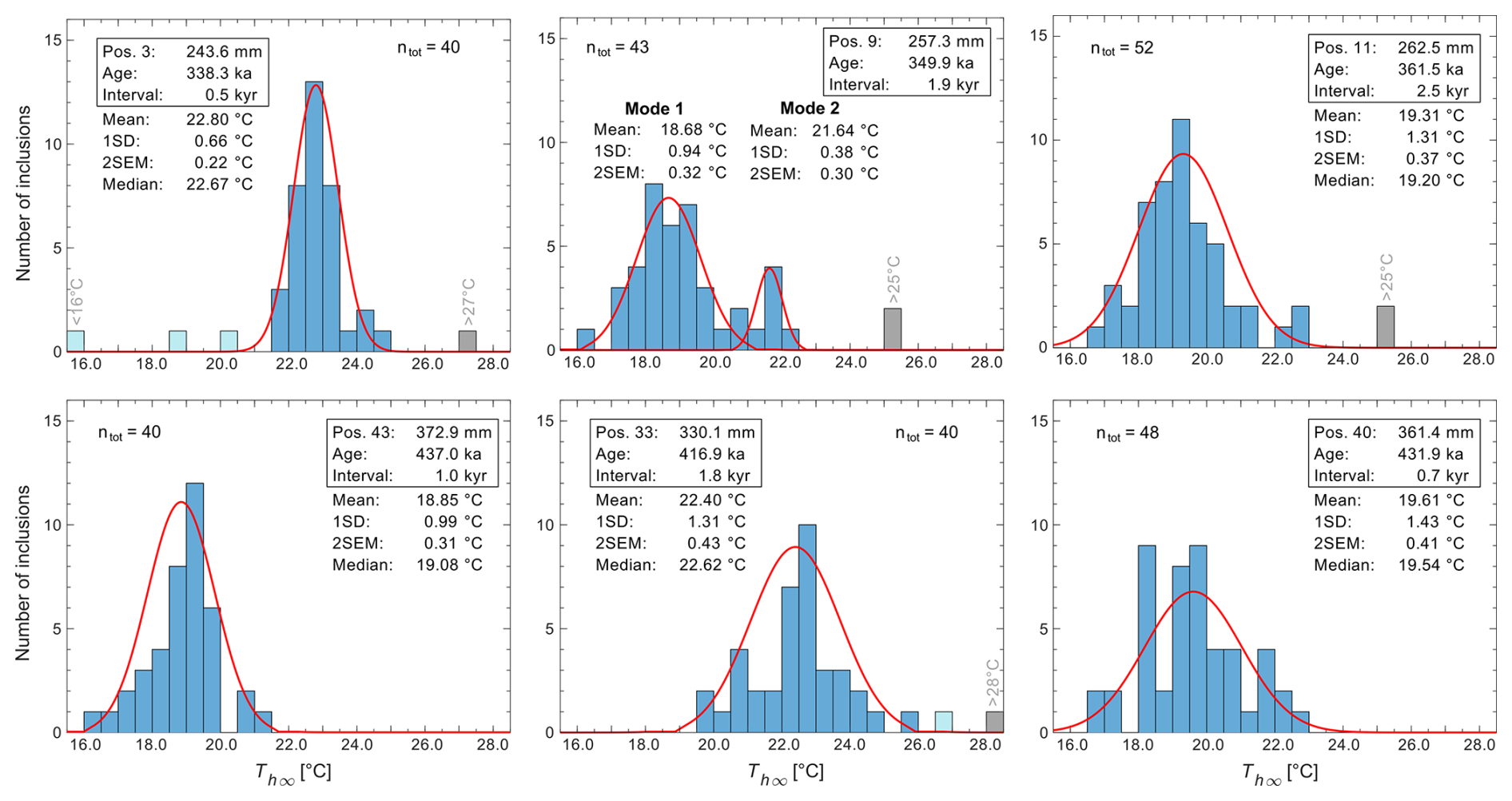
Figure 5 Selection of T_h∞ distributions obtained at different positions in stalagmite WR5_B. Inclusions that did not homogenize below a pre-defined threshold temperature are shown in grey. Values labelled in light blue are considered outliers based on a 4MAD criterion and were excluded from further statistical analyses. Red curves are Gaussian distributions fitted to the data of the remaining net sample (n_net, shown in blue) based on the mean and standard deviation (1 SD), with the mean value interpreted as cave temperature T_cave. n_tot is the total number of inclusions that were analysed. The T_h∞ distribution at sample position 9 was interpreted as bimodal and here the mean value of the dominant lower mode is considered representative for the cave temperature at the time the surrounding calcite formed (see text).

Table 1 Summary of results from WR5_B. The table lists the mean position (in mm) of the analysed growth bands relative to the isotope transect, the mean sample age and the maximum time interval covered by the sample. The statistical sample (n_stat) is the number of inclusions that homogenised below a given threshold value. Data that were rejected from the statistical sample based on a 4MAD outlier criterion are indicated in percentage. Cave temperature T_cave is defined as the average value of the respective T_h∞ distribution and reported with 1 SD and 2 SEM. Cave temperatures were finally corrected for the secondary effect of sea level-related cave altitude changes using the reconstruction of Bintanja et al. (2005) and a lapse rate of 0.6 °C/100 m (Løland et al., 2022), yielding T_corr (see Sect. 3.2).

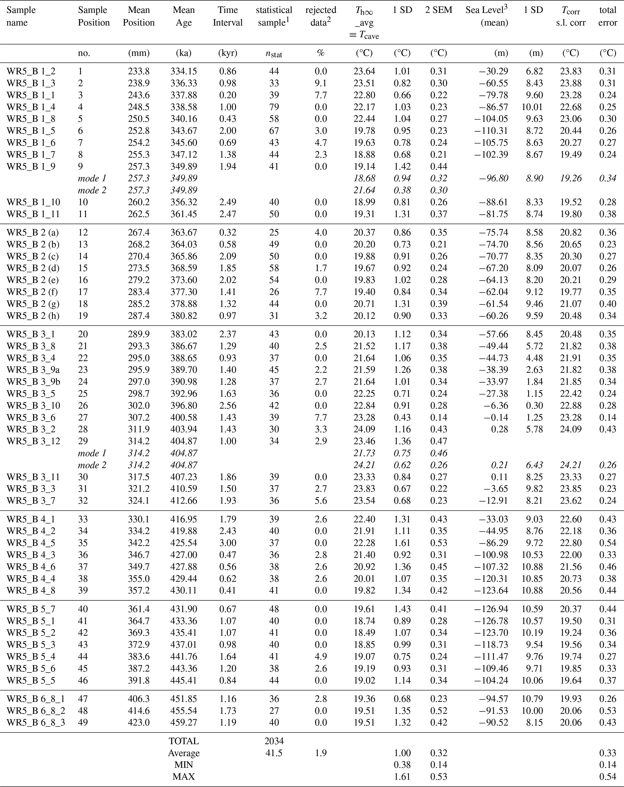
¹ statistical sample = total number of inclusions – number of inclusions with T_h(obs)> threshold value. ² recected from the statistical sample based on a 4MAD outlier criterion (Median Absolute Deviation). ³ based on the sea level reconstruction of Bintanja et al. (2005).

3 Results

3.1 Microthermometry results from individual growth bands

In the present study we analysed a total of 2090 fluid inclusions in 49 different growth bands of stalagmite WR5_B (Fig. 2) and, in addition, 146 fluid inclusions in three growth bands of stalagmite WR_MC1 (Fig. A5). In both samples as well as in other stalagmites from Northern Borneo (e.g. Løland et al., 2022), we observe a systematic scatter of T_h∞ values of 4–6 °C within individual growth bands with average standard deviations (2 SD) of 2 °C. This is about one order of magnitude larger than the analytical precision of the individual T_h∞ values and significantly larger than natural cave temperature fluctuations that can be expected for the time intervals covered by a single growth band. The reasons for this variability of T_h∞ in apparently coeval inclusions are subject of further investigations focusing on potential post-formation volume/density alterations of the inclusions and variability of the closing ages due to temporarily persisting open porosity in the calcite fabric. Most of the analysed samples display unimodal, Gaussian-like distributions of the T_h∞ values, suggesting that potential volume/density alterations affect T_h∞ randomly and thus, are not supposed to impact the accuracy of the reconstructed cave temperatures T_cave. For two of the samples, however, the T_h∞ distributions appear to be bimodal (Pos. 9 and 29). In these cases, the mean value of the dominant mode was considered representative for the stalagmite formation temperature, whereas the minor mode may result from closing ages of some of the inclusions that were significantly younger than the age of the surrounding calcite host. Standard deviations (1 SD) of the outlier-adjusted T_h∞ distributions range from 0.43 to 1.61 °C, while standard errors of the mean (2 SEM) range from 0.14 to 0.53 °C.

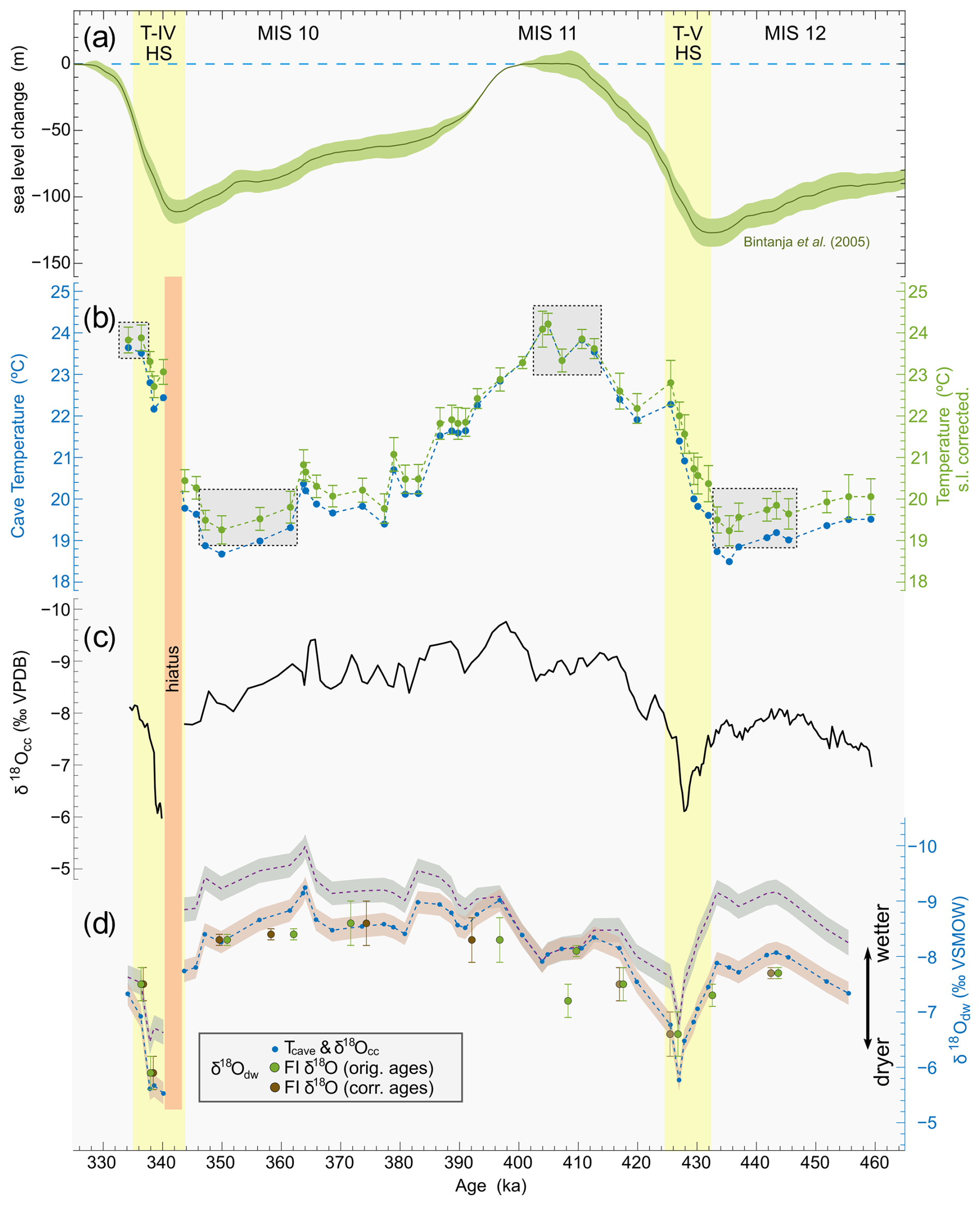
Figure 6 (a) Sea level reconstruction with 1 SD (Bintanja et al., 2005), plotted on the LR04 time scale (Lisiecki and Raymo, 2005). Note the lag of sea level rise relative to temperature at the terminations. Yellow bars indicate T-IV and T-V Heinrich stadials. (b) WR5_B temperature record (this study). Blue dots represent actual cave temperatures (T_cave) and green dots are the respective sea level corrected cave temperatures (T_corr.). For graphical reasons, error bars (2 SEM) are indicated for T_corr. only. Grey boxes indicate the T_corr. data that were used for calculating glacial and interglacial mean temperatures. (c) WR5_B oxygen isotope record (δ¹⁸O_cc) of the stalagmite calcite (Meckler et al., 2012), (d) reconstructed drip water isotope record δ¹⁸O_dw (small blue dots) derived from T_cave and δ¹⁸O_cc using the empirical calibration for oxygen isotope fractionation in speleothems of Tremaine et al. (2011) plotted with 95 % CI (light brown band). Green dots are measured δ¹⁸O_FI values from fluid inclusion water analysis based on the originally assigned sample depths (Meckler et al., 2015, data from Bern lab) with error bars indicating 1 SD of 2–3 replicate measurements. Brown dots result from the re-examination of the sample positions. The purple dashed line with the grey 95 % CI band shows the ice volume correction that shifts glacial δ¹⁸O_dw to more negative values. Note, in both (c) and (d) δ¹⁸O is plotted on reverse axes.

Reconstructed temperatures from WR5_B with statistical parameters are summarized in Table 1 along with the respective sample positions, ages, and maximum time intervals covered by each sample. For an extended data summary, including n_tot, n_net and further statistical parameters, we refer to Table S1. A selection of T_h∞ distributions at different sample positions from WR5_B is shown in Fig. 5 and histogram plots from all 49 sample positions, together with additional plots of the cumulative distribution and T_h∞-volume diagrams are provided in Fig. A4. The respective numerical data are reported in Table S2. The WR_MC1 drill core sample, on the other hand, yields an average late Holocene temperature for Whiterock Cave of 23.28 ± 0.25 °C (2 SEM), slightly lower than the present-day cave temperature of 23.7 ± 0.1 °C. The results derived from three growth bands are illustrated in Fig. A5 and numerical values are reported in Table S3. Supplementary data Tables S1–S3 are available on Zenodo.

3.2 Borneo temperature record

The reconstructed Whiterock Cave temperature record is illustrated in Fig. 6b and numerical values are reported in Table 1. Temperatures reported in this study are consistent with previous WR5_B temperature data of Meckler et al. (2015), illustrated in Fig. A6. In order to assess the amplitude of the climate-driven portion of glacial-interglacial cave temperature changes, the T_cave values were corrected to eliminate the secondary temperature effect induced by changes of the cave altitude relative to sea level that was about 120 m lower during glacial maxima. To do so, we used the global sea level reconstruction of Bintanja et al. (2005) illustrated in Fig. 6a and assumed a constant lapse rate of surface air temperatures of 0.6 ± 0.1 °C/100 m (Løland et al., 2022). The correction is largest at the glacial maxima and raises the reconstructed cave temperature by up to 0.8 °C. The temperature record shown in Fig. 6b displays both the actual cave temperatures T_cave (blue) and sea level corrected cave temperatures T_corr. (green). Propagated errors of T_corr. are up to 14 % larger than 2 SEM of T_cave at glacial maxima and include the assigned uncertainty of the lapse rate that possibly varies with climatic changes (Loomis et al., 2017), as well as uncertainties of the employed sea level reconstruction (see Table 1). A comparison of global sea level reconstructions of Bintanja et al. (2005) and Spratt and Lisiecki (2016) yielded only minor differences in the resulting temperature corrections, in spite of significant differences between the two sea level records (Fig. A7, Table S1).

The temperature record shows a clear pattern of glacial-interglacial temperature changes. Average T_corr.values during glacial maxima of MIS 12 and MIS 10 were at 19.6 ± 0.3 °C (n=6) and 19.5±0.3 °C (n=4), respectively, while average temperatures at the interglacial optimum of MIS 11 were 23.8 ± 0.3 °C (n=5), which results in an amplitude of glacial-interglacial land temperature changes of 4.2 ± 0.4 °C. Considering the extreme values only, 19.2 ± 0.4 °C (MIS 12), 24.2 ± 0.3 °C (MIS 11), and 19.3 ± 0.3 °C (MIS 10), the maximum amplitude would be 5.0 ± 0.5 °C.

The WR5_B record displays a well-resolved continuous temperature increase across the initial stage of T-V reaching a preliminary maximum at 22.8 ± 0.5 °C around 425 ka, which corresponds to a warming of 3.2 ± 0.6 °C. This initial temperature increase occurs concurrent with a strong Heinrich event (T-V HS) in the Northern Hemisphere (Vázques Riveiros et al., 2013) and a phase of deglacial drying in Northern Borneo as manifested in the stalagmite δ¹⁸O_cc signal (Fig. 6c). Since δ¹⁸O_cc and temperature were derived from the same stalagmite, we emphasize that this temporal correlation is independent of any age uncertainties. After reaching a maximum at the end of the Heinrich stadial, the temperature decreases slightly, passes a minimum, similar to the Antarctic Cold Reversal (ACR) during Termination I, and subsequently further increases towards the MIS 11 interglacial optimum. For Termination T-IV, in contrast, the recorded evolution of deglacial warming is incomplete due to a hiatus of about 3 kyr (Fig. 3). This hiatus manifests itself not only petrographically (Fig. A2a and h) but also through a clear discontinuity both in the temperature and δ¹⁸O_cc records (Fig. 6b and c). Substantial growth interruptions and/or calcite dissolution might also be the reason for very low average growth rates (0.4–0.7 µm yr⁻¹) in the run-up to T-IV. The WR5_B record ends with a deglacial temperature maximum of 23.8 ± 0.3 °C (n=2) at the end of the Heinrich stadial that coincides with the early MIS 9 interglacial optimum. Again, deglacial warming occurs during the T-IV HS, simultaneous with a pronounced excursion of the δ¹⁸O_cc signal towards more positive values, indicating drier climate. The amplitude of deglacial warming across the T-IV HS is 4.3 ± 0.4 °C, which is about 1.1 °C higher than the temperature increase across the corresponding Heinrich stadial at T-V (3.2 ± 0.6 °C).

3.3 Hydroclimate

The calcite oxygen isotope record (δ¹⁸O_cc) of stalagmite WR5_B has previously been interpreted to reflect primarily changes in hydroclimate and precipitation amount (Meckler et al., 2012) assuming that the effect of temperature on the δ¹⁸O_cc signal is relatively minor. As a side-product of this study, we employed our temperature record to calculate the oxygen isotopic composition δ¹⁸O_dw of the drip water from which the stalagmite-forming calcite precipitated. For the calculations we used the uncorrected cave temperatures T_cave and δ¹⁸O_cc together with the empirical speleothem calibration for the calcite-water oxygen isotope fractionation proposed by Tremaine et al. (2011). The calculated δ¹⁸O_dw record (Fig. 6d) agrees overall well with measured δ¹⁸O_FI values from previous fluid inclusion isotope analysis (Meckler et al., 2015). The ages of the δ¹⁸O_FI data points were adjusted according to the revised WR5_B age model. Moreover, a re-examination of the exact sample positions relative to the reference isotope transect revealed, for some of the samples, discrepancies of up 4 mm from the originally assigned sample depths. In Fig. 6d the δ¹⁸O_FI data were plotted for both the original (green dots) and the corrected sample depths (brown dots) to illustrate the resulting age shifts. We note that this reassessment of the sample positions does not affect the oxygen isotope derived temperature estimates published in Meckler et al. (2015) because the corresponding δ¹⁸O_cc values were not taken from the reference isotope transect but were measured on the crushed calcite powders remaining after fluid inclusions water isotope analysis.

The calculated δ¹⁸O_dw record was then corrected for global ice volume changes to account for changes of the sea water oxygen isotopic composition using again the sea level reconstruction of Bintanja et al. (2005) and a correction factor of 1 ‰/100 m sea level change (Schrag et al., 2002). As a result, glacial δ¹⁸O_dw shifts to more negative values (purple curve in Fig. 5d). The calculated record confirms the previous interpretation of relative drying during the T-V and T-IV Heinrich stadials inferred from δ¹⁸O_cc (Meckler et al., 2012). Moreover, in consequence of the ice volume correction, a glacial-interglacial difference in δ¹⁸O_dw arises, indicating relatively wetter conditions during the glacial periods (MIS 10 and 12) compared to the interglacial (MIS 11). We note, however, that the correction for global ice volume effect does not take potential variations in sea water δ¹⁸O in the moisture source regions into account.

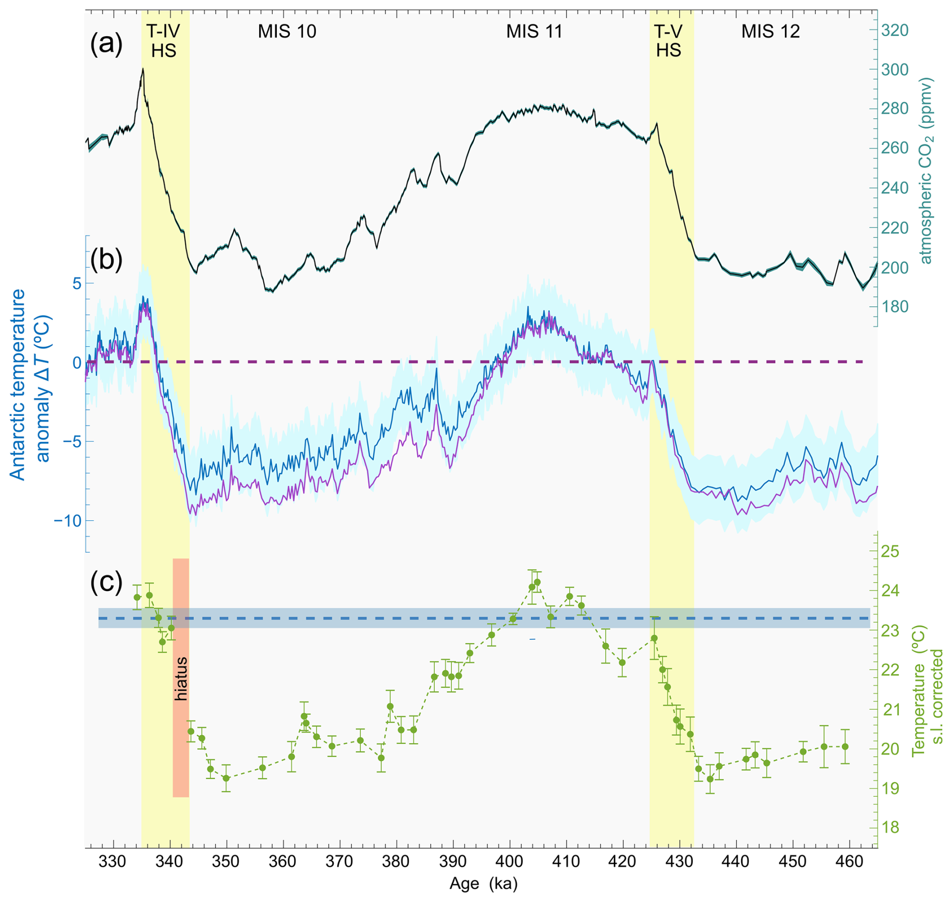
Figure 7 Comparison of the Borneo cave temperature record (T_corr.) with Antarctic ice core (EDC) records: (a) atmospheric CO₂ concentrations (Nehrbass-Ahles et al., 2020; Siegenthaler et al., 2005). (b) Antarctic temperature anomalies ΔT (purple: Jouzel et al., 2007; blue: Landais et al., 2021 with ± 2 °C uncertainty). The dashed purple line indicates ΔT=0 °C. (c) Borneo temperature record (T_corr.) derived from stalagmite WR5_B corrected for sea level-related altitude changes. The dashed blue line indicates the late Holocene reference temperature in Whiterock cave (23.3 ± 0.25 °C) determined from stalagmite WR_MC1 (Fig. A5). All EDC records are plotted on the AICC2012 ice core chronology (Bazin et al., 2013). Yellow bars indicate the T-V and T-IV Heinrich stadials.

4 Discussion

4.1 Comparison with Antarctic ice core records

Antarctic ice cores provide a wealth of different proxies for reconstructing past climate back to 800 ka. For comparison with our Borneo temperature record, we focus on two EPICA (European Project for Ice Coring in Antarctica) Dome C (EDC) ice core records, namely a recently published record of atmospheric CO₂ concentrations (Nehrbass-Ahles et al., 2020), and two temperature records: the classical EDC record of surface temperature anomalies (ΔT_s) derived from hydrogen isotope measurement of the ice, δD_ice (Jouzel et al.,2007), and a more recent ΔT_site reconstruction based on d-excess, i.e., using both δD_ice and δ¹⁸O_ice (Landais et al., 2021). These EDC records (Fig. 7a, b) were plotted on the AICC2012 time scale (Bazin et al., 2013) and demonstrate the close correlation between Antarctic temperature anomalies and atmospheric CO₂ concentrations. The CO₂ record of Nehrbass-Ahles et al. (2020) comprises a 148 kyr time interval from 297 to 445 ka, and hence, does not cover the older MIS12 period included in the WR5_B record. To fill this 15 kyr gap we used previous data from Siegenthaler et al. (2005) that were also employed for the 800 kyr CO₂ composite record of Bereiter et al. (2015). The two EDC temperature records differ systematically during glacial periods with slightly higher temperatures (smaller ΔT) in the reconstruction of Landais et al. (2021), whereas interglacial temperature anomalies are nearly identical.

Despite some age uncertainties of our Borneo temperature record, we found generally good agreement of the tropical cave temperature record with the structure of the Antarctic ΔT records. For the T-V HS, for which the uncertainties of the WR5_B age model are comparable to those of the AICC2012 ice core chronology (1.5 and 4.0 kyr, respectively), the timing of deglacial warming is nearly identical at both locations, exhibiting a maximum at the end of the Heinrich stadial, followed by a slight decrease of temperature and atmospheric CO₂. The amplitude of Antarctic temperature changes, however, is about a factor 2.3 larger compared to Borneo cave temperature (T_corr.) changes (see Sect. 4.4). The ice core records also display a series of millennial scale CO₂ and temperature fluctuations during the glacial inception and MIS 10. Similar patterns are discernible in the Borneo record; however, a clear correlation of the individual events is hampered by substantial age uncertainties in this part of the record and potential unconstrained hiatuses in the stalagmite record. For the T-IV HS, the WR5_B record provides reliable information only about the amplitude of the deglacial warming (4.3±0.4 °C) as only the high temperature end of the deglacial warming is recorded.

Peak temperatures in the EDC ΔT records for the interglacial optimum (MIS 11) and for MIS 9 (occurring at the end of the T-IV HS) were 2.5 to 3.5 °C higher than the Holocene reference value (ΔT=0, dashed horizontal line in Fig. 7b). For the Borneo record, we compared the respective peak temperatures (24.2 ± 0.3 and 23.9±0.3 °C) with the late Holocene reference temperature of 23.28 ± 0.25 °C (dashed horizontal line in Fig. 7c) derived from the drill core sample WR_MC1. We thus infer that the temperature maximum of MIS 11 was about 0.9 ± 0.4 °C warmer compared to the late Holocene, which is roughly consistent with the previously mentioned polar amplification factor of 2.3. The peak temperature at the end of T-IV, in contrast, is only 0.6 ± 0.4 °C warmer than late Holocene. To be consistent with the 3.5 °C temperature anomaly in the Antarctic record, however, one would expect the peak temperature in the cave record to be about 1.5 °C higher than the Holocene reference temperature. Although we cannot exclude that this discrepancy results from a potential attenuation of the cave temperature signal, it seems more likely that we simply missed the MIS 9 peak temperature in our record.

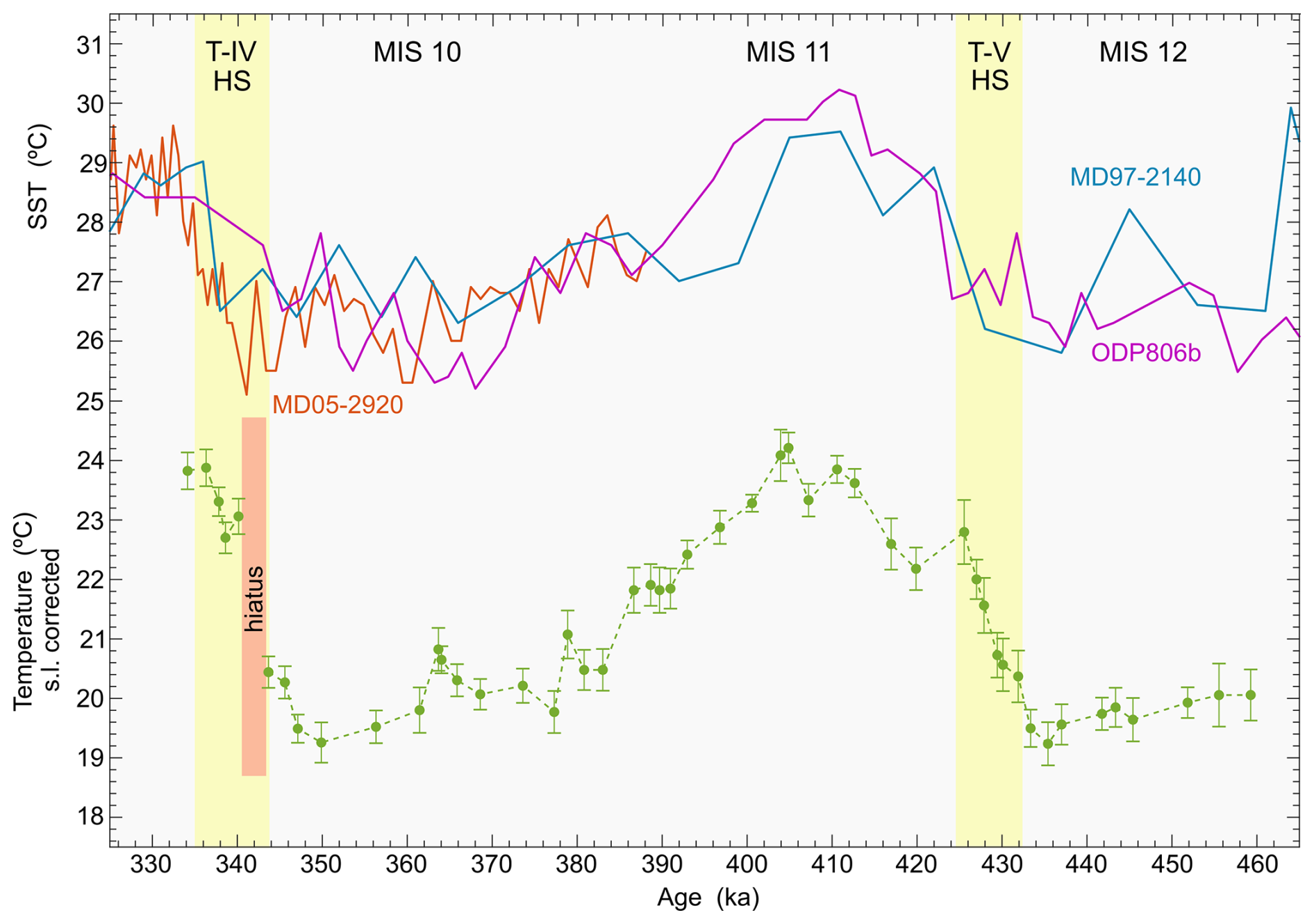
Figure 8 Comparison of the WR5_B temperature record (T_corr.) with Mg/Ca based sea surface temperatures (SSTs) from three different sites in the Western Pacific warm pool (see Fig. 1 for locations).

4.2 Comparison with sea surface temperatures (SSTs)

We compare our Borneo cave temperature record (T_corr.) with Mg/Ca based sea surface temperature (SST) records derived from three Western Pacific core sites (Fig. 8), namely ODP Site 806 (Medina-Elizalde and Lea, 2005), MD97-2140 (de Garidel-Thoron et al., 2005), and MD05-2920 (Tachikawa et al., 2014). The locations of the core sites are shown in Fig. 1. The first two records were reported on an orbitally tuned reference chronology established on ODP Site 677 (Shackleton et al., 1990), while the latter is reported on the LR04 timescale (Lisiecki and Raymo, 2005). The two SST records from Site 806 and MD97-2140 have relatively low temporal resolution but, in contrast to the higher resolved MD05-2920 record, cover the entire time interval of the WR5_B record. Although the SST data appear more variable compared to cave temperatures, partly owing to the lower temporal resolution, they clearly show the general glacial-interglacial temperature trend with differences of about 4 °C between MIS 12 and MIS 11, whereas deglacial warming across T-IV is less than 3 °C in the ODP806 and MD97-2140 records. At site MD05-2920, in contrast, the amplitude of temperature change across T-IV reaches about 4 °C, which is consistent with the amplitude obtained in the WR5_B record. In terms of absolute temperatures, it is worth noting that present-day SSTs around Northern Borneo are about 5 °C higher than cave temperatures (Meckler et al., 2015) and a similar offset is seen in the records for MIS 12-9.

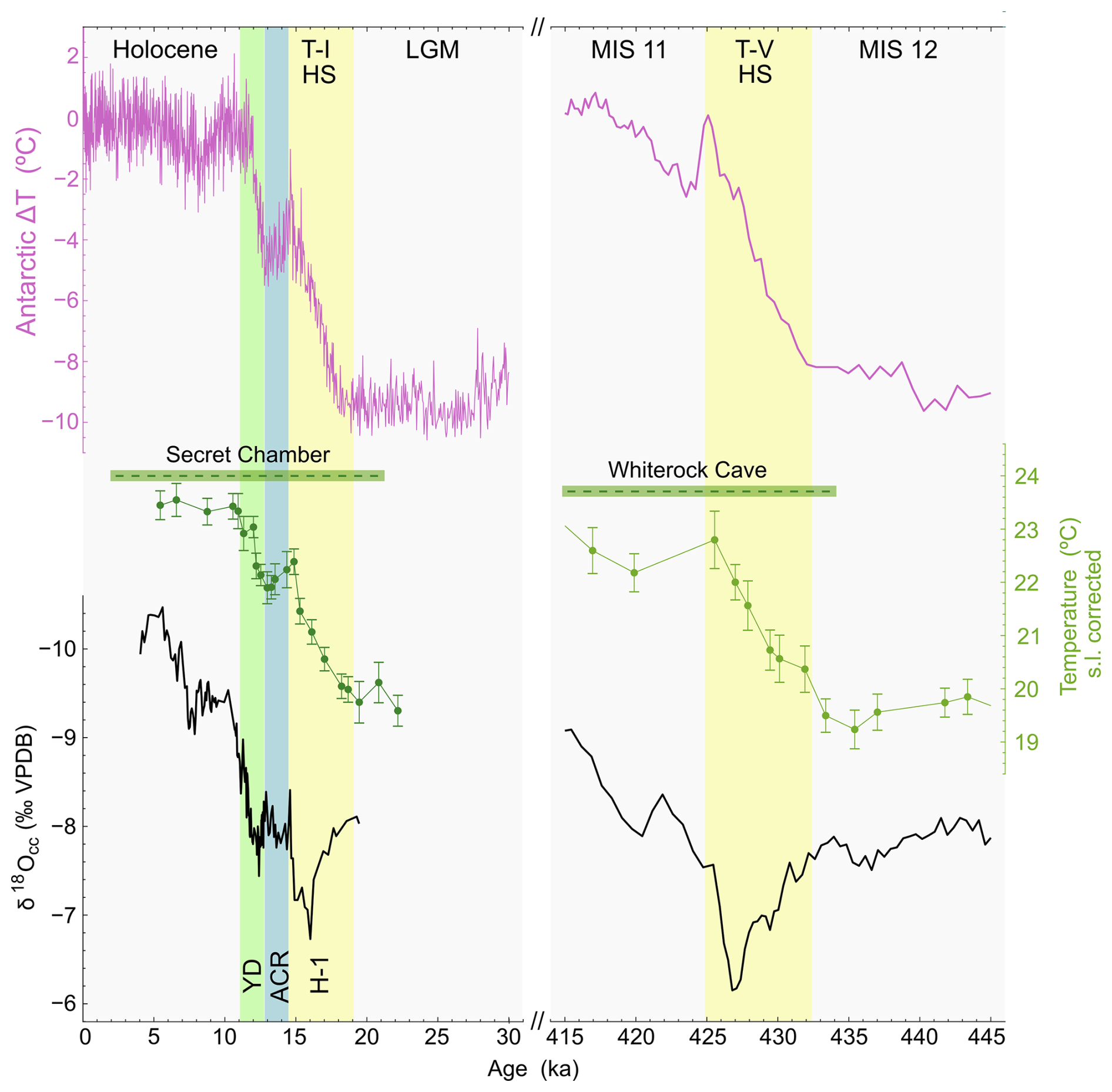
Figure 9 Comparison of T-I and T-V. Top: Antarctic temperature anomalies ΔT_s (Jouzel et al., 2007) plotted on the AICC2012 ice core chronology (Veres et al., 2013 and Bazin et al., 2013). Middle: SC02 temperature reconstruction (T_corr) across T-I (Løland et al. , 2022; not corrected for differences in cave altitude) and WR5_B record across T-V (this study). Error bars indicate 2 SEM. Dashed horizontal lines (green) indicate present-day temperatures in Secret Chamber and Whiterock Cave, respectively. Bottom: δ¹⁸O_cc records from stalagmites SC02 (Buckingham et al., 2022) and WR5_B (Meckler et al., 2012). YD: Younger Dryas, ACR: Antarctic Cold Reversal, H-1: Heinrich Stadial 1.

4.3 Comparison of T-V and T-I

Recently, Løland et al. (2022) published a cave temperature record from Northern Borneo based on fluid inclusion microthermometry covering the last glacial Termination (T-I). Stalagmite SC02 that was used for the study was collected from Secret Chamber (ca. 110 m a.s.l.), in the Clearwater cave system, which is about 8 km from Whiterock Cave. Their reconstructed temperature record (T_corr.) is shown in Fig. 9 together with calcite δ¹⁸O_cc (Buckingham et al., 2022) and the corresponding record of Antarctic temperature anomalies ΔT_s (Jouzel et al., 2007) for comparison. When compared to our new temperature reconstruction across T-V, the two records exhibit the same structure and timing. Both show an early deglacial warming starting at the beginning of Heinrich stadials, a preliminary maximum at the end of the Heinrich events, followed by a slight temperature decrease and a subsequent recovery. At T-I, the excursion of δ¹⁸O_cc to more positive values, indicating relatively drier conditions, is clearly related to the H-1 interval and the analogous behaviour is observed during the Heinrich stadial at T-V. The similar pattern of early deglacial warming concurrent with relative drying in Borneo during deglacial Heinrich events, when the Northern Hemisphere cools, corroborates the finding of Løland et al. (2022) that during deglaciations, the temperature evolution in Northern Borneo proceeds in step with Southern Hemisphere temperature and atmospheric CO₂ concentrations while hydroclimate is affected by Northern Hemisphere cooling.

Early deglacial warming in Antarctica has been attributed to the classical seesaw behaviour, with heat release or accumulation in the Southern Ocean caused by a weakening of the Atlantic Meridional Overturning Circulation (AMOC) associated with reduced heat transport to and deep ocean ventilation in the North (e.g., Broecker, 1998; Pedro et al., 2011). The subsequent slight cooling (e.g., during the ACR) then corresponds to the re-establishment of the AMOC. The fact that the same relative timing of deglacial warming can also be observed in tropical Borneo demonstrates that the temperature response to a reduced AMOC is not restricted to the high southern latitudes and Antarctica.

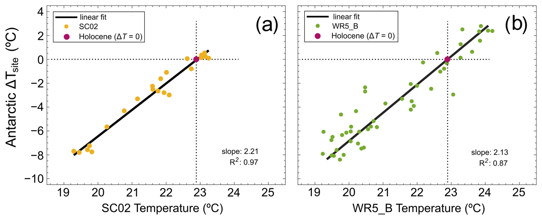
Figure 10 Correlations between Antarctic temperature anomalies ΔT_site (Landais et al., 2021) and (a) altitude- and sea level corrected cave temperature data (T_corr., n=22) derived from stalagmite SC02 (Løland et al., 2022) covering the time interval from 23–6 ka and (b) sea level corrected cave temperatures (T_corr., n=49) derived from stalagmite WR5_B (this study) covering the time interval from 460-333 ka. The slopes of the regression lines represent polar (Antarctic) amplification factors and the purple dots at ΔT_site=0 are resulting predictions of average late Holocene Borneo temperatures. Due to the higher temporal resolution of the Antarctic record, we employed a Gaussian filter with a bandwidth (1 SD) of 0.2 kyr to obtain representative Antarctic temperature values.

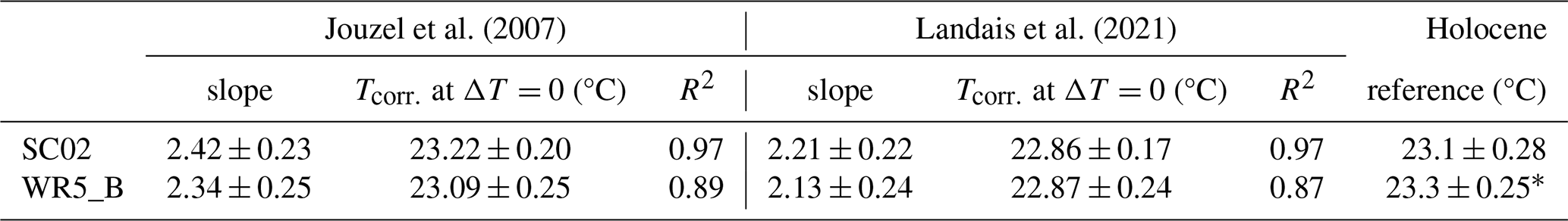
Table 2 Correlations between Borneo cave temperature records (T_corr.) and Antarctic temperature anomalies ΔT. The slopes of the linear regression lines (Figs. 10a, b and A8a, b) represent empirical estimates of polar amplification factors while the respective intercepts at Antarctic ΔT=0 are equivalent to Holocene Borneo temperatures estimates (both given with 95 % confidence interval (CI)). Holocene temperatures (with 2 SEM) derived from stalagmite SC02 and from the drill core sample^* (WR_MC1) collected in Whiterock Cave (Fig. S5) are shown in the rightmost column for comparison.

The amplitude of deglacial warming in Northern Borneo during H-1 was 2.6±0.3 °C, compared to 3.2 ± 0.6 °C during the corresponding Heinrich stadial at T-V, while the total temperature increase from the Last Glacial Maximum (LGM) to the early-to-mid Holocene amounts to 3.6 ± 0.3 °C (Løland et al., 2022), compared to 4.2 ± 0.4 °C from MIS 12 to the MIS 11 temperature optimum. When correcting SC02 temperatures for the difference in cave altitude (70 m) between Secret Chamber and Whiterock Cave by 0.3 ± 0.14 °C based on the offset of present-day cave temperatures (24.0 ± 0.1 and 23.7 ± 0.1 °C, respectively), the altitude-corrected early-to mid-Holocene average temperature from SC02 would be 23.1 ± 0.28 °C, and thus 1.1±0.4 °C colder than the MIS 11 temperature optimum derived from WR5_B. This is in line with the temperature difference of 0.9 ± 0.4 °C between MIS11 and the late Holocene reference temperature (23.3 ± 0.25 °C) determined for Whiterock cave (see Sect. 4.1) and demonstrates the consistency of the reconstructed temperature data across different stalagmites and caves. Using the same 0.3 centigrade altitude correction, the average LGM temperature derived from SC02 decreases to 19.5 ± 0.35 °C (n=3), equivalent to the average temperatures at the glacial maxima of MIS 12 (19.6±0.3 °C; n=6) and MIS 10 (19.5 ± 0.3 °C; n=4). While our new record reveals warmer interglacial temperatures during MIS11 compared to the Holocene, there is no significant temperature difference between the three glacial maxima, which is in line with Antarctic ΔT reconstructions.

4.4 Polar amplification

The two Borneo temperature records from SC02 (Løland et al., 2022) and WR5_B (this study) show clear linear correlations with Antarctic temperature anomalies both from Landais et al. (2021) and Jouzel et al. (2007), illustrated in Figs. 10a, b and A8a, b, respectively, where the slope of the regression line reflects a site-specific Antarctic amplification factor, i.e., the ratio between East Antarctic (Dome C) and Borneo cave temperature (T_corr.) changes ($\mathrm{\Delta }{T}_{\mathrm{Antarctic}}/\mathrm{\Delta }{T}_{\mathrm{Borneo}}$). For simplicity, age and temperature uncertainties of the records were not considered for the fits. We found very strong correlations between Antarctic ΔT and the SC02 record (R²=0.97) and slightly weaker correlations for the WR5_B record (R²=0.87 and 0.89, respectively; see Table 2). The weaker correlation of the WR5_B record likely relates to larger age uncertainties. The slopes of the regression lines differ insignificantly between the SC02 and WR5_B records, but they reflect the systematically higher glacial temperatures in the Antarctic ΔT reconstruction of Landais et al. (2021) compared to that of Jouzel et al. (2007). The intercepts of the regression lines at Antarctic ΔT=0 closely accord with stalagmite-derived average Holocene temperatures from SC02 and WR_MC1. We note that SC02 temperatures used for the linear fits were corrected for the altitude difference between Secret Chamber and Whiterock Cave (see Sect. 4.3). The strong correlation between the Borneo and the Antarctic records that were derived from different climate archives with independent temperature proxies can be taken as evidence for the reliability of these paleo-temperature reconstructions.

5 Conclusions

The present study provides a new cave temperature record from tropical Northern Borneo derived from speleothem fluid inclusions covering the time interval between 460 and 333 ka ago. Our results reinforce the great potential of NA microthermometry for obtaining highly precise and accurate paleo-temperature data, indicated by small standard errors and the consistency of temperature data across different stalagmites and records from other archives. Based on our results we suppose that the delay of the cave temperature response to surface air temperature changes is too short to affect the amplitude of the cave temperature signal on millennial and glacial-interglacial timescales. A potential systematic offset of cave and surface air temperature, however, cannot be excluded yet, and if we assume variability of this temperature offset over time, for example, due to changes in precipitation amount, this could result in minor modifications (both increase or decrease) of the temperature amplitude in the cave.

Our record shows that Borneo cave temperatures evolved in step with changes in Southern Hemisphere (Antarctic) temperature across T-V and T-IV, corroborating previous findings of Løland et al. (2022) observed for the last glacial termination (T-I). Just as during T-I, deglacial warming starts with the beginning of Heinrich stadials involving relative drying in Northern Borneo and cooling in the Northern Hemisphere. We thus confirm a widespread warming effect of the deglacial AMOC reduction, as well as a clear decoupling between temperature and hydroclimate in the West Pacific Warm Pool region during deglacial Heinrich events.

We find a strong linear correlation between Antarctic ΔT and the two Borneo records, SC02 (LGM to Holocene; Løland et al., 2022) and WR5_B (MIS 12 to MIS 9; this study), yielding statistically indistinguishable polar amplification factors, which raises the question whether polar (Antarctic) amplification can, as a first order approximation, be assumed constant over the past 460 kyr. Further temperature records from Borneo stalagmites covering other time intervals at higher temporal resolution and with better age constraints than WR5_B will allow testing this hypothesis and investigating the sensitivity of tropical cave temperatures to short-term millennial scale climate fluctuations. In addition, these records may also provide insights in lag times and signal attenuation across sub-millennial temperature changes.

Appendix A: Supplementary figures

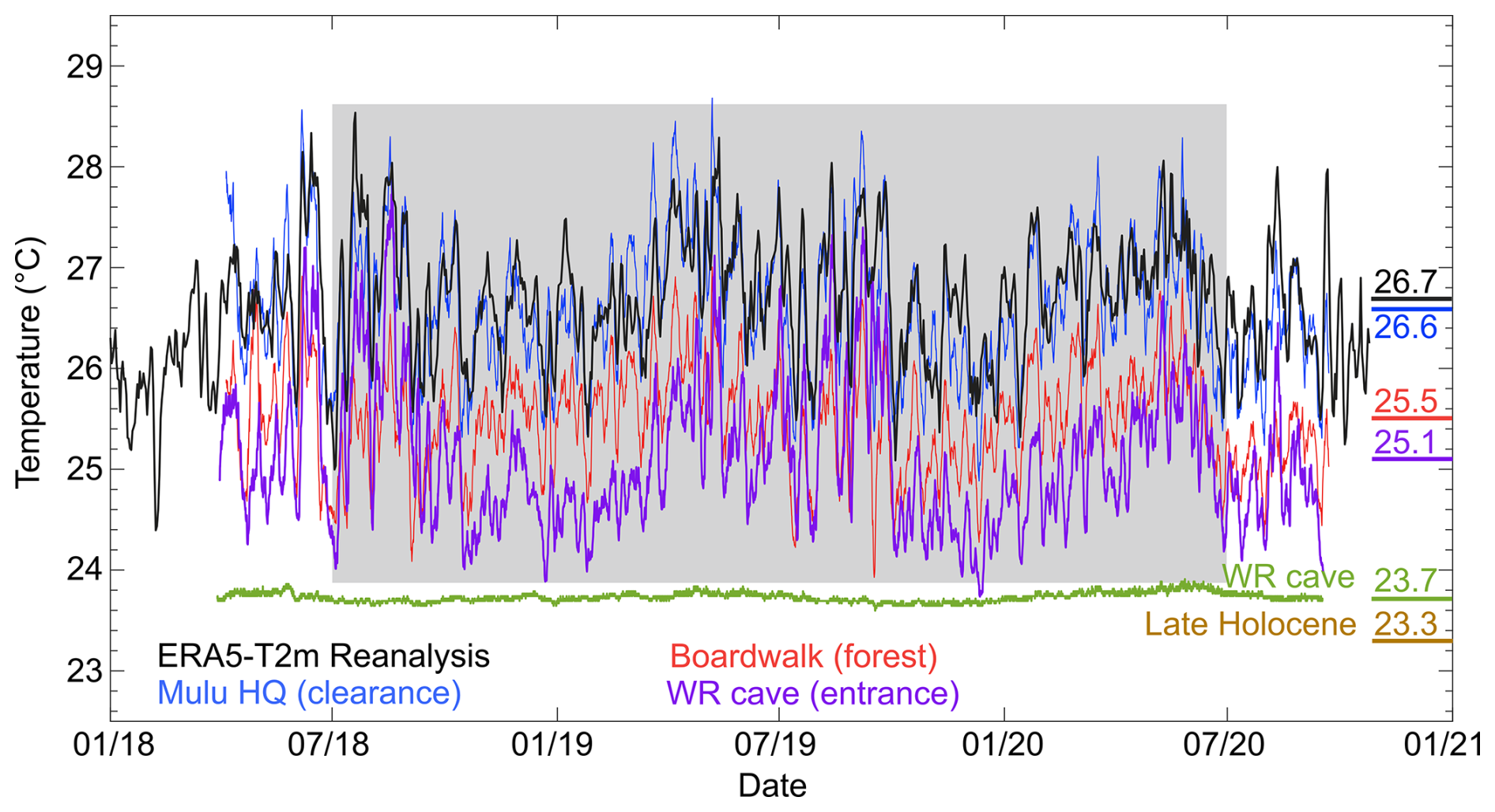
Figure A1 Surface and cave air temperatures recorded between March 2018 and September 2020. Blue: Mulu Park head quarter (HQ), located in a forest clearance about 30 m a.s.l.; red: location along the tourist boardwalk in the forest (30 m a.s.l.; purple: Whiterock “midnight” cave entrance (180 m a.s.l.); black: ERA-5 T2m temperature reanalysis for the area (3.85–4.25° N, 114.60–114.85° E); green: Whiterock cave temperature. Average temperatures over a 2-year period (grey box) are shown on the right of the respective records. In addition, the reconstructed late Holocene reference temperature from the WR_MC1 drill core sample is indicated in brown.

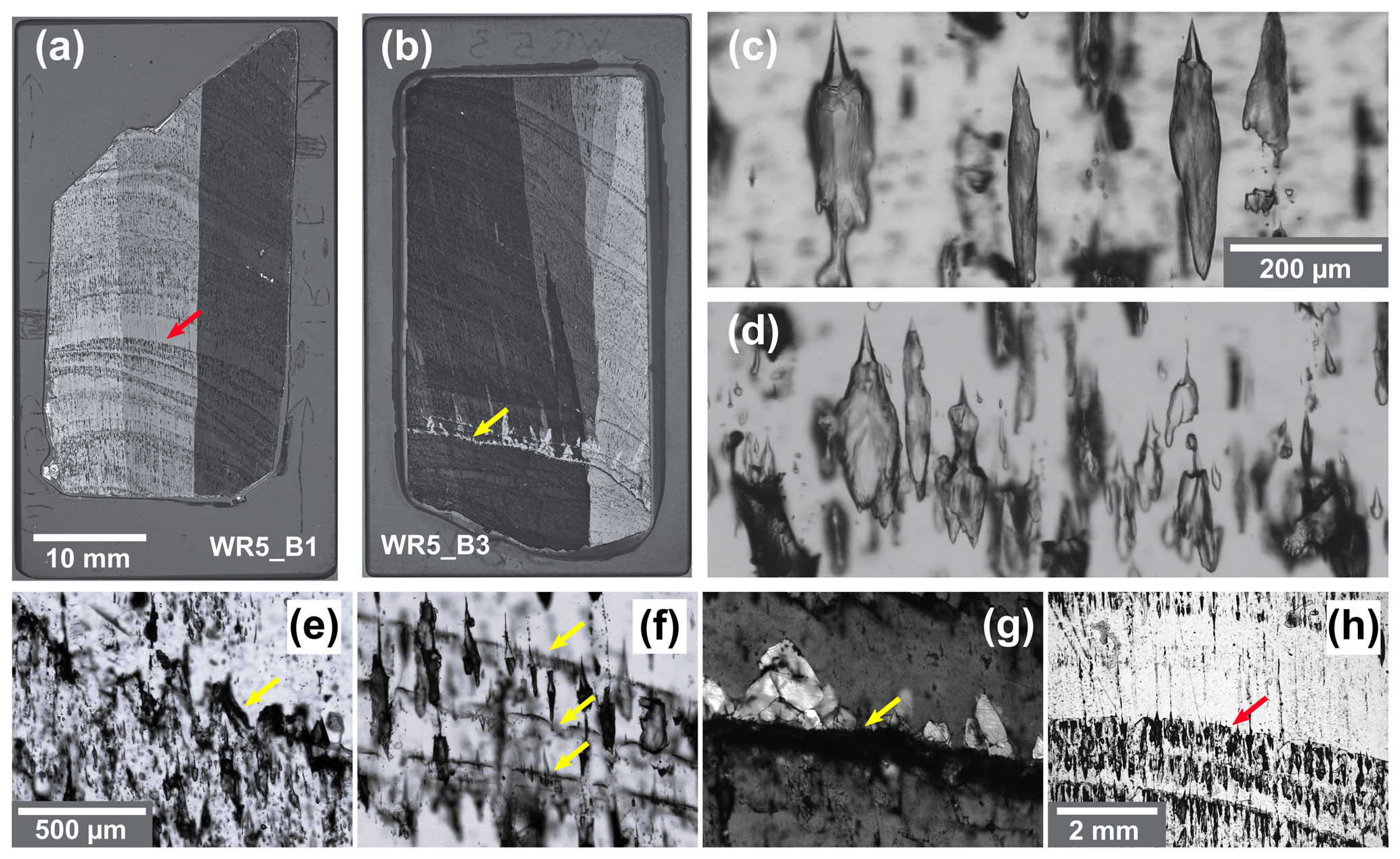
Figure A2 (a, b) Polished stalagmite thick sections (ca. 200 µm) viewed in transmitted light with partly crossed polarizers. The calcite fabric is characterized by large composite crystals that are built up from columnar crystal units of nearly uniform c-axis orientation. Arrows indicate the growth hiatuses shown in (h) and (g), respectively. (c, d) monophase liquid fluid inclusions of various shapes and sizes. The inclusions are typically located between adjacent columnar crystal units and are elongated parallel to the calcite c-axis and growth direction, respectively. (e) Hiatus with dissolution features (Type E surface). (f) Hiatus with even surface that is outlined with countless tiny sub-micron inclusions. (g) Calcite crystals with random crystallographic orientation on the hiatus surface shown in (b). (h) Enlarged image of the prominent hiatus at the beginning of T-IV shown in a) and marked with a red line in Fig. 2. Sample positions 5 and 6 (Table 1) are right above and below the hiatus, respectively.

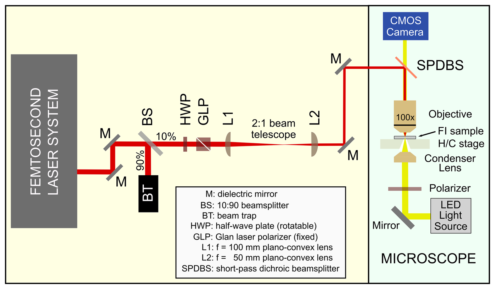
Figure A3 Schematic representation of the analytical setup used for NA microthermometry. The femtosecond laser system (CPA-2101, Clark-MXR, Inc.) provides ultra-short laser pulses with a nominal pulse width of 150 fs (1 fs $={\mathrm{10}}^{-\mathrm{15}}$ s) and an output power of ca. 0.9 W at 1 kHz repetition rate. For NA microthermometry the output power is attenuated to ca. 20 mW and the laser is operated in single pulse mode. The laser wavelength is 775 nm and accordingly, NIR-coated optics are used to direct the laser beam to the microscope. Via two dielectric mirrors (M) the beam passes a 10:90 beamsplitter (BS), transmitting only 10 % of the laser light, while reflecting 90 % into a beam trap (BT). After this second attenuation step, the beam passes a rotatable half-wave plate (HWP) and a fixed Glan laser polariser (GLP). Rotation of the HWP by 45° changes the polarisation direction of the laser from horizontal to vertical and in combination with the fixed GLP the laser power can be further attenuated and fine-tuned. After the polariser the laser beam passes a 2:1 beam telescope consisting of two plano-convex lenses (L1 and L2) with focal lengths of 100 and 50 mm, respectively. The beam telescope reduces the beam diameter to ca. 3 mm and re-collimates the beam before it is coupled into the microscope light path by means of two more mirrors (M) and a short-pass dichroic beamsplitter (SPDBS, Chroma ZT720spxxr-uv-UF1) that is mounted in a dual port intermediate tube on the microscope. The dichroic beamsplitter reflects the 775 nm wavelength of the laser into the microscope objective and transmits the visible spectral range from the microscope illumination below ca. 700 nm. Kinematic mirror mounts are used to couple the laser beam properly into the microscope light path. The microscope (Olympus BX53) is equipped with a Linkam THMSG600 heating/cooling stage, an Olympus LMPLFLN $\mathrm{100}\times /\mathrm{0.8}$ long working distance objective (WD: 3.4 mm) and a digital monochrome camera (pco.edge 3.1). For microthermometry the 100× objective is placed into a metal jacket that fits through an open lid on the Linkam stage, sealed with rubber o-rings.

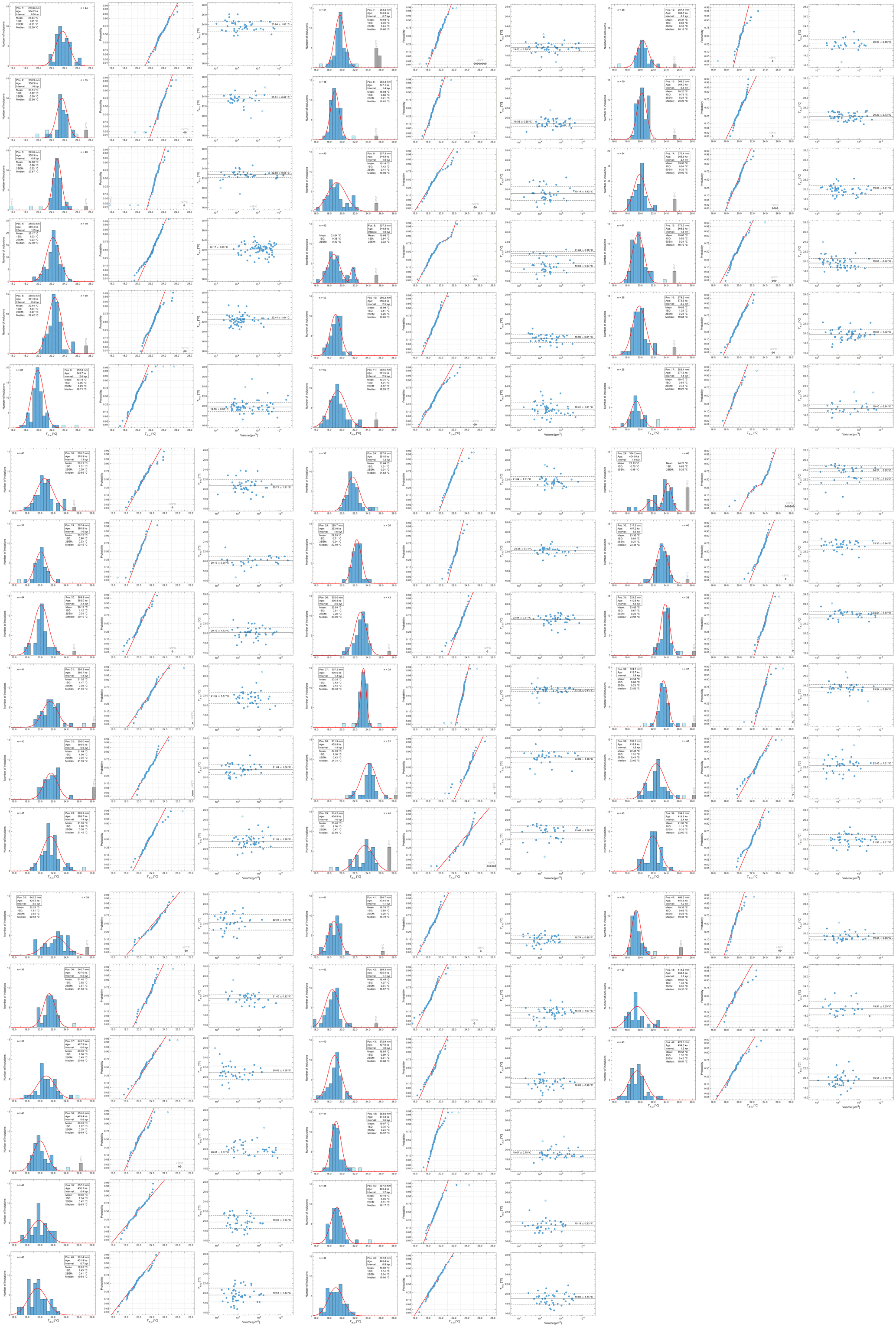
Figure A4 WR5_B data plots for sample positions 1–49. Left column: histogram plots of T_h∞. Inclusions with T_h(obs) greater than the threshold value are marked in grey, T_h∞ values that were classified as outliers based on a 4MAD criterion are marked in light blue and were not considered for statistical analysis. Red curves are Gaussian fits to the data based on the mean and standard deviation (1 SD) of the distribution; n= total number of inclusions, SEM = standard error of the mean. At positions 9 and 29 the T_h∞ distributions were considered as bimodal based on statistical tests. For comparison, we also provide the respective unimodal fits to the data. Centre column: cumulative distribution plots of the T_h∞ data. Note the straight red line represents the same Gaussian function as in the histogram plots but now plotted on a logarithmic probability scale. Right column: T_h∞-V plot illustrating the size range of the analysed inclusions and the scatter of the T_h∞ values in the individal samples. Note, there is no correlation between T_h∞ and inclusion volume, confirming that the observed scatter of T_h∞ is volume independent. Grey line: mean; dashed black lines: ± 1 SD. Numerical values are reported in Table S2.

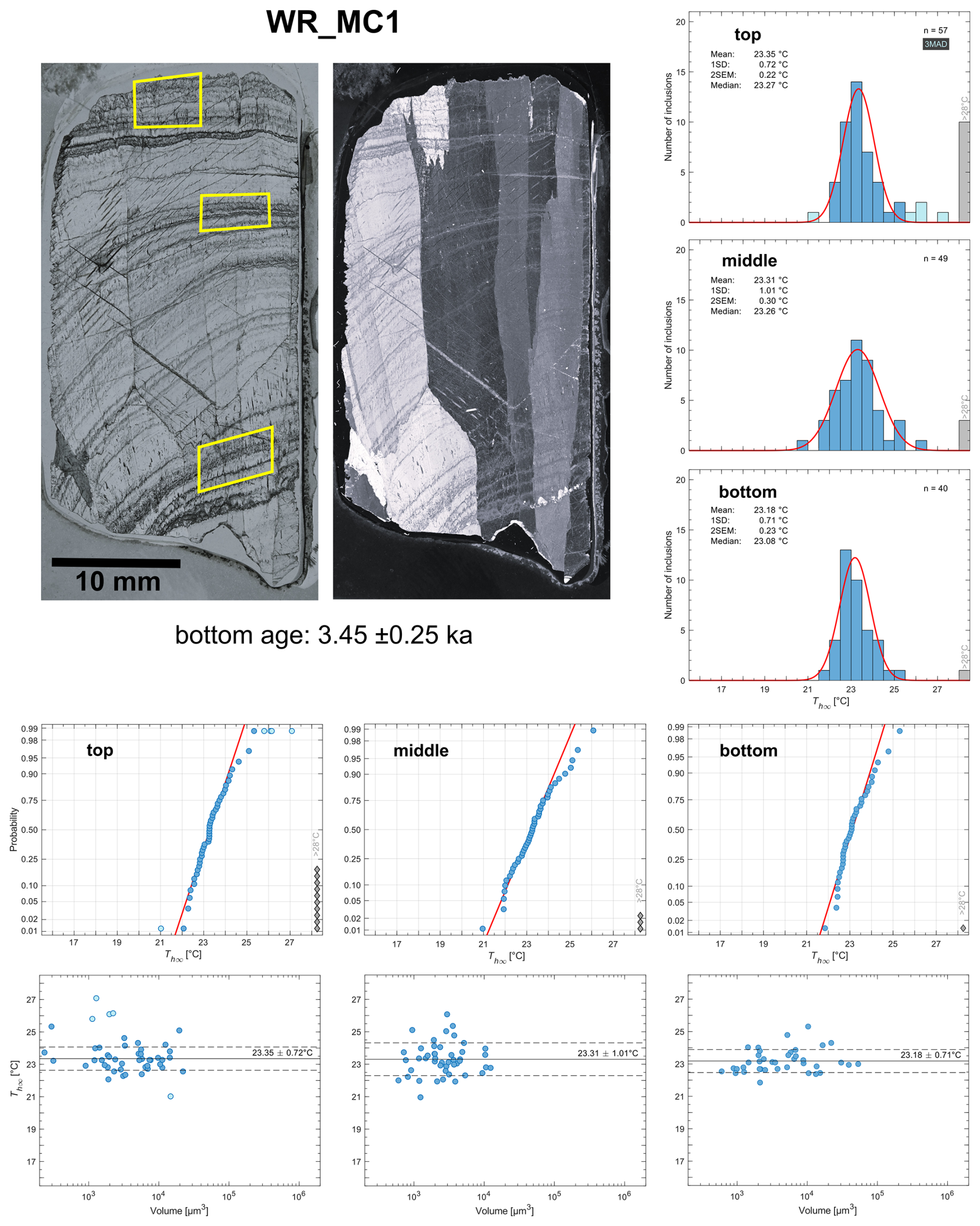
Figure A5 Drill core sample WR_MC1 taken from an actively growing stalagmite covering the Late Holocene (bottom age: 3.45 ± 0.25 ka). Upper panels: Left: image of the thick section in transmitted plane polarised light. Fluid inclusions were analysed at the three sample positions indicated on the image. Middle: same section viewed in cross-polarised light, showing the large domains of uniform c-axis orientation of the columnar calcite fabric. Right: histogram plots of the T_h∞ distributions for the three sample positions. Note, for the top sample we used a 3MAD instead of the common 4MAD outlier criterion to get rid of the extreme values of the high-temperatures tail. Lower panels: cumulative distribution plots of the T_h∞ data and T_h∞-V diagrams. Numerical values are reported in Table S3.

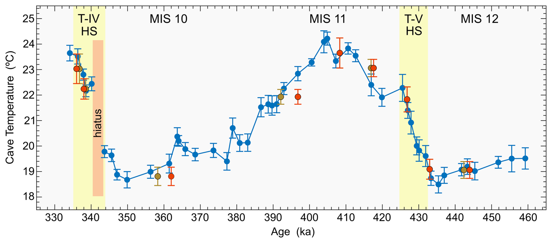
Figure A6 Comparison of WR_5B temperatures (T_cave) from this study (blue) with previously published data (red; Meckler et al., 2015). To compare the two data sets, we reassessed the exact sample positions of the previous data points to check for consistency with the present record (cf. Sect. 3.3). For some samples deviations of the originally assigned sample depths were found to be up to 4 mm. Sample ages are based on the revised age model and in the diagram, we show them for both original (red) and the corrected (brown) sample depths.

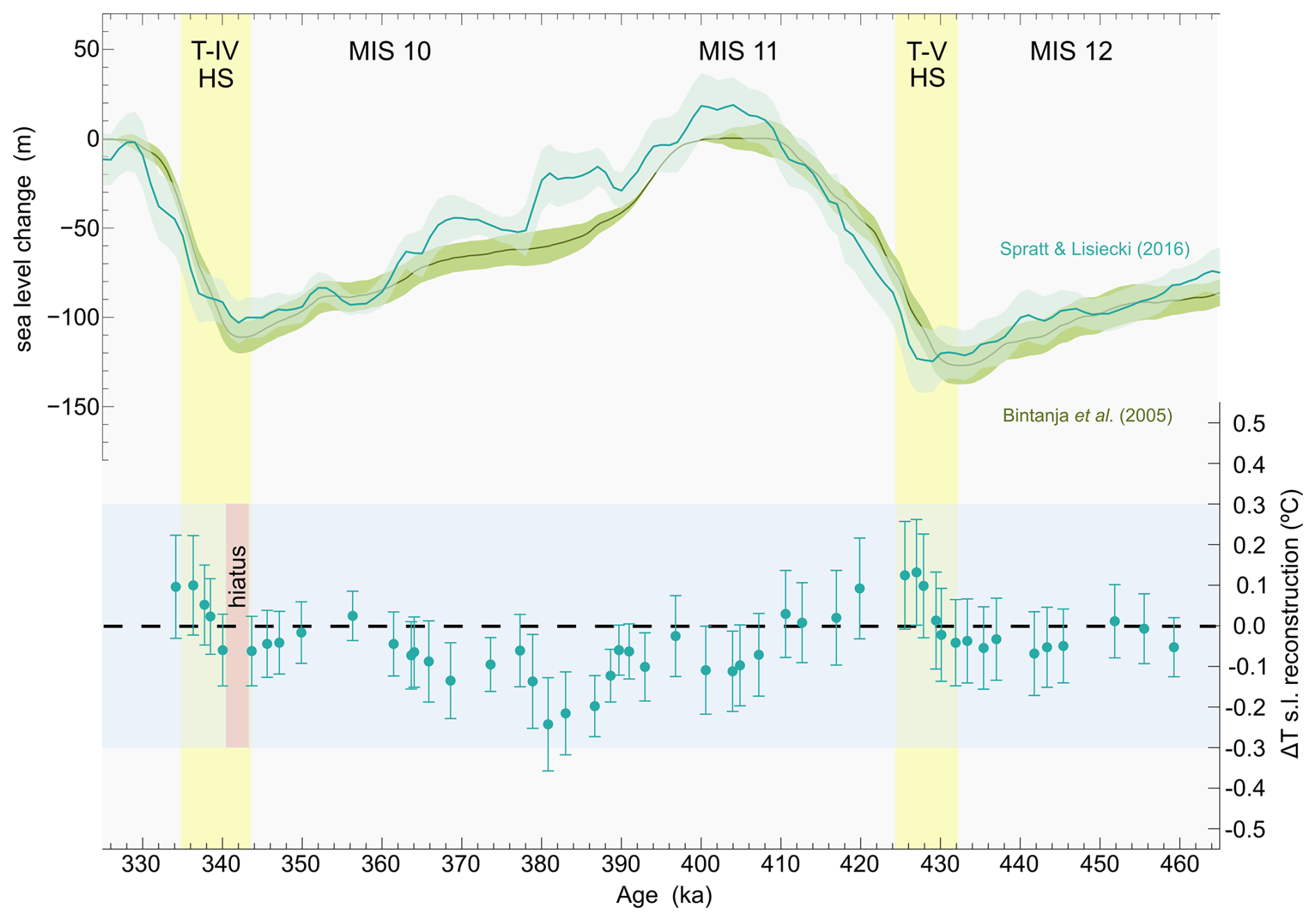
Figure A7 Top: Comparison of sea level reconstructions from Bintanja et al. (2005) and Spratt and Lisiecky (2016) plotted on the LR04 time scale (Lisiecki and Raymo, 2005). Note, the lag of sea level rise with respect to deglacial warming at the T-V and T-IV Heinrich stadials indicated with yellow bars. The lag is more pronounced in the record of Spratt and Lisiecky (2016) that, in addition, features more variability during the glacial inception from MIS 11 to MIS 10, which is in accordance with millennial scale climate variations observed in the Antarctic temperature and CO₂ records. Bottom: Differences in sea level corrected Borneo land temperatures T_corr depending on the chosen sea level reconstruction (cf. Table S1). ΔT becomes largest at the Terminations and during the glacial inception with error bars relating to the uncertainty (1 SD) of the sea level estimates. The variation of ΔT is within a bandwidth of ± 0.3 °C (blue shaded area), and thus, within the average error (2 SEM) of the reconstructed T_corr values.

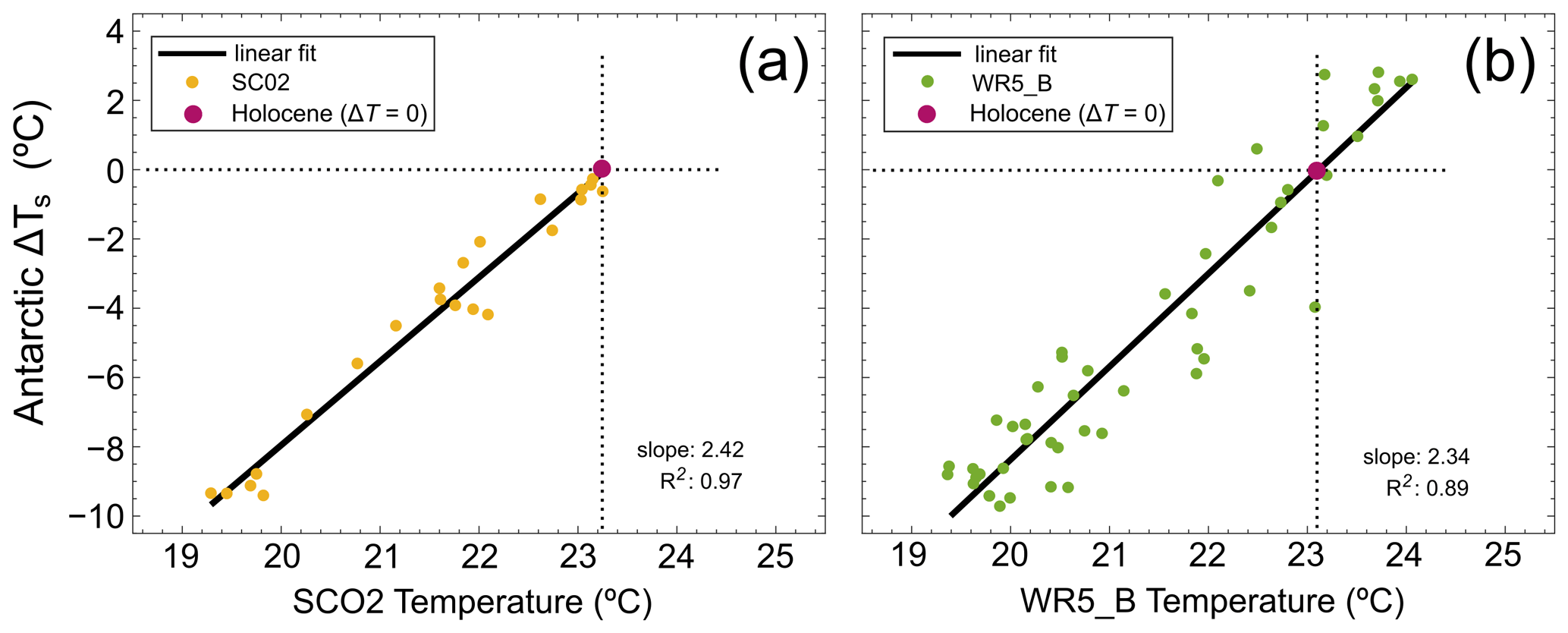
Figure A8 Correlations between Antarctic temperature anomalies ΔT_s (Jouzel et al., 2007) and (a) altitude- and sea-level corrected SC02 temperatures (Løland et al., 2022) covering the time interval from 23–6 ka and (b) sea level corrected WR5_B temperatures (this study) covering the time interval from 460–333 ka. The slopes of the regression lines represent polar (Antarctic) amplification factors and the purple dots at ΔT_s=0 are resulting predictions of average late Holocene Borneo temperatures.